The Euler characteristic of graph complexes via Feynman diagrams
Abstract.
We prove several claims made by Kontsevich about the orbifold Euler characteristic of the three types of graph homology introduced by him. For this purpose, first we develop a simplified version of the Feynman diagram method, which requires integrals in one variable only, to obtain the generating functions as asymptotic expansions of certain Gaussian integrals. Finally, following Penner, we relate these integrals to the gamma function in order to compute the individual coefficients of the generating functions.
1. Introduction
In two papers ([10], [11]) published in 1993 and 1994, Kontsevich constructed a family of objects called graph complexes. These are chain complexes of vector spaces, where each vector space is spanned by a set of finite graphs equipped with an orientation. He computed the orbifold Euler characteristic of these chain complexes, and stated the answers; however, he did not give any proofs except for a one sentence reference to Feynman diagrams.
In Sections 5, 6 and 7 we recall the definitions of the graph complexes and their orbifold Euler characteristic, and prove most of Kontsevich’s claims about them. But first, we introduce the two technical tools used in the proof. In Section 3, we develop a simplified version of the Feynman diagram apparatus (also called the method of Gaussian integrals). This method, well known to physicists but mostly unknown to mathematicians, can be used to construct generating functions for various problems involving the counting of graphs. A good exposition of the general method can be found in [4]. Our version is based on [15]. It is limited in that it cannot take into account the number of boundary components of ribbon graphs (referred to as the “topological expansion” in the physics literature), but it is much simpler as it requires integration over only, instead of over a space of matrices. In Section 4, we recall some basic facts about asymptotic expansions, which are used to extract information about the individual terms of the generating functions obtained by the Feynman diagram method.
The emphasis is on proving the claims made by Kontsevich about the orbifold Euler characteristic of the commutative, associative and Lie graph complexes. However, our simplified Feynman diagram method can be applied to graph complexes based on other cyclic operads (see [5] or [13]), as well as to other problems involving the counting of graphs.
2. Acknowledgements
This work has grown out of a seminar organized by Karen Vogtmann in Fall 2000 at Cornell University, with the goal of understanding Kontsevich’s graph homology. It is based on Chapter 5 of the author’s Ph.D. dissertation, which could not have been written without Swapneel Mahajan’s help.
3. Enumeration of graphs
As our first example, we consider the following counting problem. Let be the set of graphs with edges such that each vertex has valence at least 3. (The valence of a vertex is the number of edges incident to it.) For each , let be the set of automorphisms of . The goal is to evaluate the sum
| (3.1) |
The first observation is that we are, in fact, counting the number of labeled graphs. We will say that a graph with edges is labeled if the half-edges are numbered from through (see Figure 1). Fix a graph , and consider all its labelings, i.e., the (isomorphism classes of) labeled graphs with as the underlying unlabeled graph. The symmetric group acts on these labelings, and the size of the stabilizer of any given labeling is equal to the number of automorphisms of . Thus if denotes the set of labeled graphs with edges such that each vertex is at least trivalent, then
| (3.2) |
i.e., the sum to be computed is the number of labeled graphs divided by .
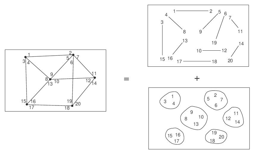
Second, notice that we can break up a labeled graph into two separate objects: a pairing of the numbers , , …, , which we will call a chord diagram, describes the edges; and a partition of these numbers into groups of three or more tells us what the vertices are. Conversely, any pair of a chord diagram and such a partition corresponds to a labeled graph. Therefore, if denotes the number of chord diagrams on numbers and the number of set partitions of distinct objects into subsets of size three or more, then
| (3.3) |
Each of the quantities on the right hand side are fairly easy to compute. In the case of chord diagrams, this could be done directly, but in both cases the simplest solution is to find their exponential generating functions and .
Namely, let denote some class of objects; following [9], we will call it a species. Let be the corresponding exponential generating function, where is the number of objects of type on numbers, vertices etc. Consider the exponential species , the objects of which are the disjoint unions of any number of objects of type . Then the exponential generating function is equal to the formal exponential
| (3.4) |
of the power series , provided that any object of type can be uniquely decomposed into its sub-objects of type . In particular, we must have , so the sum above is finite in each coefficient. This is an application of Joyal’s theory of combinatorial species; details can be found in [3] or [12].
Now, let be the species of two-element sets, i.e., and for all . The exponential generating function is . On the other hand, we have , and thus
| (3.5) |
Similarly, if denotes the species of sets of size greater than or equal to three, then we have
| (3.6) |
Since , we immediately obtain
| (3.7) |
Finally, we would like to find the exponential generating function of , given those of and , using equation (3.3). This is called the Cartesian product of the two species, denoted by . There does not seem to be any general method for computing the generating function of a Cartesian product; however, in this particular case, when one of the factors is , the following lemma solves the problem. Readers familiar with the the theory of Feynman diagrams will recognize it as a one-dimensional version of the calculation underlying Wick’s Lemma.
Lemma.
.
Proof.
Straightforward. ∎
Another way of stating the lemma is
| (3.8) |
Note that this formula holds for odd values of , as well: in this case, both sides are zero. If we could exchange the order of the summation and the integration, we would have
| (3.9) |
Although this formula needs explanation (the series does not converge: its radius of convergence is zero), it is indeed valid in a limited sense, as we shall see below.
4. Asymptotic expansions
Power series with zero radius of convergence can be treated analytically by considering them as the asymptotic expansion of some function. We briefly recall the definition and basic properties of asymptotic expansions; details can be found in [6], for example.
Definition.
Let be a function defined on a subset of including a (possibly one-sided) neighborhood of 0, with values in or . We say that the formal power series is an asymptotic expansion of around and we write
| (4.1) |
if the following condition is satisfied for each :
| (4.2) |
This means that for each fixed , the quotient is bounded in some neighborhood of .
Note that the neighborhoods we take in (4.2) may shrink down to zero as , in which case our definition does not say anything about the tail of the series for any fixed non-zero . It is possible that , but the series does not converge for any non-zero value of . Even when the series does converge, its sum is not necessarily equal to ; for example, as . Also note that the function does not need to be differentiable, or even continuous.
On the other hand, if is a function, and its Taylor series has a positive radius of convergence, then the Taylor series is an asymptotic expansion of . A function may not have an asymptotic expansion, but if it does, it is unique: one can show by induction on (4.2) that the two series are equal term by term. All the usual operations on formal power series carry over to asymptotic expansions: given the asymptotic expansions of and , the functions , , etc. all have asymptotic expansions, which are equal to the sum, product, exponential etc. of those of and , as formal power series.
If we consider it as an asymptotic expansion, any power series can be exchanged with the integral in the Lemma of the previous section. More precisely, the following is true.
Proposition.
Suppose that has the asymptotic expansion around zero , and the integral converges for all in some neighborhood of zero. Then has the following asymptotic expansion around zero:
| (4.3) | ||||
Proof.
Since , we have
| (4.4) | ||||
| (4.5) | ||||
| (4.6) | ||||
| (4.7) |
because is finite for any fixed value of . ∎
Or in other words:
Theorem 1.
Let be any species. If there is a function such that is the asymptotic expansion of around zero, then
| (4.8) |
as long as the the integral converges for all in some neighborhood of zero.
We will also need the following more general version, which can be proved in the same way.
Corollary.
Let be defined on , where is some neighborhood of zero, and suppose there is a sequence of polynomials such that
| (4.9) |
holds for each , where is an integer depending only on . Suppose further that the integral converges for all . Then has an asymptotic expansion around zero, which can be obtained from (4.9) by replacing each occurrence of by the number .
5. The orbifold Euler characteristic
Our goal is the compute the orbifold Euler characteristic of certain graph complexes. A graph complex is a chain complex
where each is a vector space (in this paper, always over ) spanned by some set of graphs. In our examples, graphs in have vertices. Given a graph complex of finite length where each is spanned by a basis corresponding to the finite list of graphs , , , , its orbifold Euler characteristic is defined as
| (5.1) |
Or, if is the set of all the graphs and is the number of vertices of the graph , then we can write
| (5.2) |
Let be the graph complex where is spanned by all graphs of valence 3 or more on vertices such that the number of edges minus the number of vertices is . (If the graph is connected, this means that there are independent loops in the graph, i.e., the fundamental group of the graph has rank .) We want to compute the generating function
| (5.3) |
of the orbifold Euler characteristic of this graph complex.
First, consider the power series
| (5.4) |
and replace each occurrence of by the number (note that this eliminates all the odd powers of ). We get a power series in and , which is almost the same as the series considered in Section 3, but with an extra for each vertex of the graphs. More precisely, the coefficient of is the sum over graphs with edges and vertices.
Now, substitute to obtain the power series
| (5.5) |
If we substitute for each occurrence of , we get a power series in , where the coefficient of is the sum over graphs with . Note that ensures that all the exponents of are non-negative, and that if we order by exponents of , then the coefficient of is a polynomial in , with exponents between and .
So we have proved the following: if we replace each occurrence of by in the power series defined above in (5.5), we get times the generating function .
Now it is a simple matter to check that the conditions of the Corollary to Theorem 1 are satisfied, and hence
| (5.6) |
The same method works for many different types of graph complexes.
Theorem 2.
Consider the graph complex consisting of graphs with some structure at each vertex, represented by the species Q, where is spanned by all such -graphs on vertices. If , then the orbifold Euler characteristic of the graph complex can be obtained from the power series
| (5.7) |
by replacing each occurrence of by .
6. The three graph homologies
In [10], Kontsevich constructed three graph complexes, spanned by what we will call commutative, associative and Lie graphs. The homology of the chain complex, i.e., the quotient is Kontsevich’s graph homology.
Commutative graphs are the simplest: they are finite graphs of valence 3 or higher, i.e., of the type considered so far. The species at each vertex is . Classes in commutative graph homology play a role in the theory of finite type invariants of homology 3-spheres [2].
Associative graphs have the additional structure of a cyclic ordering of the half-edges at each vertex. These are the same as the ribbon graphs or fat graphs of Teichmüller theory. Associative graph homology is the direct sum of the homology of certain moduli spaces of mapping class groups [5]. The species at each vertex is , the species of cyclic orderings; its terms are .
Lie graphs have a planar trivalent tree at each vertex, subject to some relations corresponding to the anti-symmetry and Jacobi identity of Lie algebras. The corresponding graph homology computes the homology (with trivial real coefficients) of the group . The details can be found in [5]; for now we only need the number (more precisely: the dimension of the quotient vector space) of such trees with leaves, which is .
Other types of graph homologies can also be considered, and Kontsevich’s machinery, including the Euler characteristic computations explained here, can be applied to them; but only these three are known so far to have applications in other parts of mathematics.
There are two complications. First, Kontsevich considers connected graphs only, thereby obtaining the primitive homology of the corresponding topological object. This is easy to remedy: the logarithm of the generating function for the orbifold Euler characteristic of all graphs yields that of connected graphs only.
The second problem is that Kontsevich’s graphs come with a sense of orientation, and the chain groups are spanned by those graphs only which do not have any orientation-reversing automorphisms. By a lucky coincidence, in the associative and Lie cases, removing the graphs with orientation-reversing automorphisms does not change the homology or the orbifold Euler characteristic; this is shown in [5]. In the commutative case, unfortunately, it does: already in the case of 3 independent loops, we get if we include graphs with orientation-reversing automorphisms, and if we do not. According to Kontsevich, we do get an approximately correct answer, though, because the typical graph does not have any automorphisms.
| orbifold Euler characteristic | |||
|---|---|---|---|
| # loops | (commutative) | (associative) | (Lie) |
| 2 | |||
| 3 | |||
| 4 | |||
| 5 | |||
| 6 | |||
| 7 | |||
| 8 | |||
| 9 | |||
| 10 | |||
| 11 | |||
Table 1 shows the orbifold Euler characteristics , and of Kontsevich’s commutative, associative and Lie graph complexes, respectively, for small numbers of independent loops. The results are after taking the logarithm, but without removing graphs with orientation-reversing automorphisms. It was computed using (5.7) and the computer algebra software Mathematica.
A striking feature of this “experimental data” is the equality of the commutative and the associative orbifold Euler characteristics. Furthermore, if we type these numbers into the On-Line Encyclopedia of Integer Sequences [14], we find that
| (6.1) |
where the are the Bernoulli numbers. By using asymptotic expansions, we can prove these facts.
Remark.
The numbers in Table 1 are not new. The associative case (including (6.1) for ) follows from Harer and Zagier’s computations [8] of the Euler characteristic of mapping class groups; the power series was computed by Smillie and Vogtmann [16] as the generating function of the orbifold Euler characteristic of . Our paper confirms their computations by describing another, simpler, derivation of these results.
7. Evaluating the integrals
The following computation in the commutative case is the same as Penner’s [15]. The other two sections are (unfortunately incomplete) attempts at extending his method to the associative and Lie graph complexes, as well.
7.1. The commutative case
The commutative series is the Taylor expansion of around . We can apply Theorem 2 directly with , which gives us
| (7.1) | ||||
Here we substituted . Now substitute to obtain
| (7.2) | ||||
where in the last step we applied the integral formula which is one of several equivalent definitions of the gamma function. It is well known that has the asymptotic expansion around infinity given by Stirling’s formula
| (7.3) |
(see, for example, [1]), where
| (7.4) |
and the are the Bernoulli numbers. If we apply this formula to , take the logarithm, and compare terms, we get
| (7.5) |
In other words, the orbifold Euler characteristic of is zero for odd, and it is given by (7.5) for . Note that our notation for the Bernoulli numbers assumes
| (7.6) |
This seems to be standard, but it is different from the notation in [1].
7.2. The associative case
The associative series is the Taylor expansion of around , which is undefined when . However, the Taylor expansion of is , and satisfies the conditions of the Corollary to Theorem 1. Since the odd powers of are eliminated, Theorem 2 yields
| (7.7) |
Now we can write
| (7.8) | ||||
where the logarithm function is defined on the complex plane minus the positive real axis. Next, we substitute to get
| (7.9) | ||||

where is the curve which comes from above the positive real axis, goes around the origin counter-clockwise, and goes back to below the real axis.
This contour integral is related to the gamma function via Hankel’s formula
| (7.10) |
see, for example, [17], section 12.22. Applying this formula, together with the identity
| (7.11) |
to our integral, we get
| (7.12) | ||||
This is exactly the negative of the expression (7.2) we got in the commutative case! Hence, if we substitute back in place of , we get the same orbifold Euler characteristic
| (7.13) |
for the associative graph complex as for the commutative graph complex. (Which, however, is not the exact answer in the commutative case, as we have noted earlier.)
7.3. The Lie case
I do not know yet how to deal with this case. The Lie series is the Taylor expansion of around , which is once again not defined for , but is. Therefore, in the same way as in the associative case, from Theorem 2 we get
| (7.14) | ||||
where . If we now substitute , we obtain
| (7.15) |
I do not know whether this integral can be related to some known asymptotic series, like in the other two cases; but even if it can not, we might be able to use it to extract some information about the coefficients of .
8. Summary and further questions
We have derived Kontsevich’s formula (5.8) using the method of Feynman diagrams and the theory of asymptotic expansions. Using these techniques, one could also compute the orbifold Euler characteristic of other graph complexes, as stated in Theorem 2.
I have written a Mathematica notebook which performs this computation; it can be downloaded from http://www.math.cornell.edu/Research/Dissertations/Gerlits/code. One enters the formula for on the second line of the notebook, executes each of the subsequent lines, and the output of the last line is the orbifold Euler characteristic of the -graph complex for independent loops. The numbers in Table 1 were generated by this notebook.
For example, one could consider the “chord diagram graph complex” by putting a chord diagram at each vertex. Then , and the generating function of the orbifold Euler characteristic is
Kontsevich claims that in the Lie case, one gets even larger numbers for the orbifold Euler characteristic than the Bernoulli numbers which show up in the other two cases. This ought to be able to be proved using (7.15); also, one should be able to give a direct proof for the fact that the orbifold Euler characteristic of the associative graph complex is zero when the number of loops is odd. Another direction would be to try to incorporate Kontsevich’s orientation into the Feynman diagram apparatus so that we could exclude graphs with orientation-reversing automorphisms, and compute the actual orbifold Euler characteristic in the commutative case, as well as for graph complexes based on other species.
References
- [1] L. V. Ahlfors. Complex analysis. McGraw-Hill Book Co., New York, third edition, 1978.
- [2] D. Bar-Natan, S. Garoufalidis, L. Rozansky, and D. P. Thurston. The Århus integral of rational homology 3-spheres. I. A highly non trivial flat connection on . Selecta Math. (N.S.), 8(3):315–339, 2002.
- [3] F. Bergeron, G. Labelle, and P. Leroux. Combinatorial species and tree-like structures. Cambridge University Press, Cambridge, 1998.
- [4] D. Bessis, C. Itzykson, and J. B. Zuber. Quantum field theory techniques in graphical enumeration. Adv. in Appl. Math., 1(2):109–157, 1980.
- [5] J. Conant and K. Vogtmann. On a theorem of Kontsevich. Algebr. Geom. Topol., 3:1167–1224 (electronic), 2003.
- [6] N. G. de Bruijn. Asymptotic methods in analysis. Dover Publications Inc., New York, third edition, 1981.
- [7] F. Gerlits. Invariants in chain complexes of graphs. PhD thesis, Cornell University, Ithaca, NY, 2002.
- [8] J. Harer and D. Zagier. The Euler characteristic of the moduli space of curves. Invent. Math., 85(3):457–485, 1986.
- [9] A. Joyal. Une théorie combinatoire des séries formelles. Adv. in Math., 42(1):1–82, 1981.
- [10] M. Kontsevich. Formal (non)commutative symplectic geometry. In The Gel’fand Mathematical Seminars, 1990–1992, pages 173–187. Birkhäuser Boston, Boston, MA, 1993.
- [11] M. Kontsevich. Feynman diagrams and low-dimensional topology. In First European Congress of Mathematics, Vol. II (Paris, 1992), pages 97–121. Birkhäuser, Basel, 1994.
- [12] J. H. van Lint and R. M. Wilson. A course in combinatorics. Cambridge University Press, Cambridge, 1992.
- [13] S. Mahajan. Symplectic operad geometry and graph homology. Available electronically at arXiv:q-alg/0211464, 2002.
- [14] The On-Line Encyclopedia of Integer Sequences. Published electronically at http://www.research.att.com/˜njas/sequences/, 2003. Sequence ID A046969.
- [15] R. C. Penner. Perturbative series and the moduli space of Riemann surfaces. J. Differential Geom., 27(1):35–53, 1988.
- [16] J. Smillie and K. Vogtmann. A generating function for the Euler characteristic of , in: Proceedings of the Northwestern conference on cohomology of groups (Evanston, Ill., 1985). J. Pure Appl. Algebra, 44(1–3):329–348, 1987.
- [17] E. T. Whittaker and G. N. Watson. A course of modern analysis. Cambridge University Press, Cambridge, 1996.