Span of the Jones polynomialof an alternating virtual link

Let $D$ be an unoriented virtual link diagram. The replacement of the diagram in a neighborhood of a real crossing as in Figure 2 are called A-splice and B-splice, respectively [7, 8].

A state  of $D$ is a virtual link diagram obtained from $D$ by doing A-splice or B-splice at each real crossing of $D$. The Kauffman bracket polynomial $\langle D\rangle$ of $D$ is defined by

where $S$ runs over all states of $D$, $\natural(S)$ is the number of A-splice minus that of B-splice used to obtain the state $S$, and $\sharp(S)$ is the number of loops of $S$.

For an oriented virtual link diagram $D$, the writhe $\omega(D)$ is the number of positive crossings minus that of negative crossings of $D$. The $f$-polynomial of $D$ is defined by

For a virtual link $L$ represented by $D$, the $f$-polynomial $f_{L}(A)$ of $L$ is defined by $f_{D}(A)$. When $L$ is a classical link, the $f$-polynomial $f_{L}(A)$ is equal to the Jones polynomial $V_{L}(t)$ after substituting $A^{4}$ for $t$.

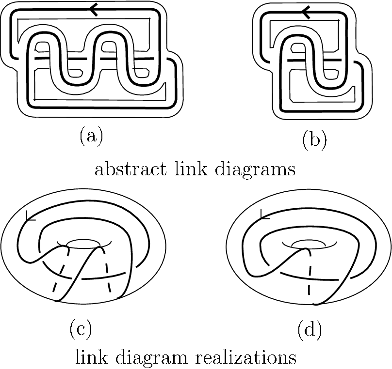
A pair $P=(\Sigma,{\cal D})$ of a compact oriented surface $\Sigma$ and a link diagram ${\cal D}$ in $\Sigma$ is called an abstract link diagram (ALD) if $|{\cal D}|$ is a deformation retract of $\Sigma$, where $|{\cal D}|$ is a graph obtained from ${\cal D}$ by replacing each crossing with a vertex. If ${\cal D}$ is an oriented link diagram, then $P$ is said to be oriented. Unless otherwise stated, we assume that an ALD is oriented. If $|{\cal D}|$ is connected (or equivalently, $\Sigma$ is connected), then $P$ is said to be connected. Two examples of connected ALDs are illustrated in Figure 3 (a) and (b).

Let $P=(\Sigma,{\cal D})$ be an ALD. For a closed oriented surface $F$, if there exists an embedding $h\co\Sigma\longrightarrow F$, then $h({\cal D})$ is a link diagram in $F$. We call $h({\cal D})$ a link diagram realization of $P=(\Sigma,{\cal D})$ in $F$. Figure 3 (c) and (d) are link diagram realizations of the ALDs illustrated in Figure 3 (a) and (b), respectively.

The supporting genus $g(P)$ of $P=(\Sigma,{\cal D})$ is the minimal genus of a closed oriented surface in which $\Sigma$ can be embedded [5].

Let $D$ be a virtual link diagram. Consider a link diagram realization $\cal D$ of $D$ in a closed oriented surface $F$ and take a regular neighborhood $N({\cal D})$ of $\cal D$ in $F$. Then $(N({\cal D}),{\cal D})$ is an ALD. We call it the ALD associated with $D$, and denote it by $\phi(D)$. (Note that $\phi(D)$, up to homeomorphism, does not depend on the choice of $F$ and the realization $\cal D$ in $F$.) An easy method to obtain $\phi(D)$ is illustrated in Figure 4 (see [5] for details). For example, the ALDs illustrated in Figure 3 (a) and (b) are the ALDs associated with the virtual link diagrams in Figure 5 (a) and (b), respectively.

Let $P=(\Sigma,{\cal D})$ be an ALD. A crossing $p$ of ${\cal D}$ is proper if four connected components of $\partial\Sigma$ passing through the neighborhood of $p$ are all distinct. See Figure 6. When every crossing of $\cal D$ is proper, we say that $P$ is proper. Let $D$ be a virtual link diagram and $\phi(D)=(\Sigma,{\cal D})$ the ALD associated with $D$. A real crossing of $D$ is said to be proper if the corresponding crossing of ${\cal D}$ is proper. A virtual link diagram $D$ is said to be proper if each crossing of $D$ is proper (or equivalently if $\phi(D)$ is a proper ALD).

The left hand side of Figure 7 is a proper alternating virtual link diagram and the right hand side is a non-proper virtual link diagram. The right hand side is a v-alternating virtual link diagram obtained from the left diagram by virtualizing a real crossing.

Let $P=(\Sigma,{\cal D})$ be an ALD. We say that $P$ is chekerboard colorable if we can assign two colors (black and white) to the region of $\Sigma\setminus|{\cal D}|$ such that two adjacent regions with an arc of $|{\cal D}|$ have distinct colors, where $|{\cal D}|$ is the graph obtained from $\cal D$ by assuming each crossing to be a vertex of degree four. A checkerboard coloring of $P$ is such an assignment of colors.

If $P$ is an alternating ALD, then it has a checkerboard coloring such that for each crossing, the regions around each crossing are colored as in Figure 8. (This fact is seen as follows: Walk on any knot component of $\cal D$ and look at the right hand side. When we pass a crossing as an over-arc, or as an under-arc, the right is colored black, or white respectively. Since $\cal D$ is alternating, we have a coherent coloring.) We call such a coloring a canonical checkerboard coloring of an alternating ALD, which is unique unless $P$ has a connected component without crossings.

Let $P=(\Sigma,{\cal D})$ be an ALD and let ${\cal S}_{A}$ (or ${\cal S}_{B}$, resp.) be the state of $\cal D$ obtained from $\cal D$ by doing A-splice (resp. B-splice) for every crossing. (See Figure 9. The states on $\Sigma$ are no longer ALDs.)

Suppose that $P=(\Sigma,{\cal D})$ be alternating, and consider a canonical checkerboard coloring of $P$. Then $(\Sigma,{\cal S}_{A})$ and $(\Sigma,{\cal S}_{B})$ inherit checkerboard colorings. See Figure 10. Black regions of $(\Sigma,{\cal S}_{A})$ are annuli. Thus we have a one-to-one correspondence

so that a loop of ${\cal S}_{A}$ and the corresponding loop of $\partial\Sigma$ bound an annulus colored black. Similarly, white regions of $(\Sigma,{\cal S}_{B})$ are annuli. Thus we have a one-to-one correspondence

so that a loop of ${\cal S}_{B}$ and the corresponding loop of $\partial\Sigma$ bound an annulus colored white. Thus we have the following.

We have an example of an alternating ALD with a canonical checkerboard coloring and the states ${\cal S}_{A}$ and ${\cal S}_{B}$ in Figure 11.

We denote the maximal (or minimal, resp.) degree of a Laurent polynomial $\eta$ by ${\rm maxd}(\eta)$ (resp. ${\rm mind}(\eta)$). For a state $S$ of a virtual link diagram $D$, let $\langle S|D\rangle$ stand for $A^{\natural S}(-A^{2}-A^{-2})^{\sharp S-1}$.

For non-zero integer $r_{1},\cdots,r_{s}$, we denote by $K(r_{1},\cdots,r_{s})$ a virtual link diagram illustrated in Figure 16. The virtual link represented by this diagram is also denoted by $K(r_{1},\cdots,r_{s})$. M. Murai [12] proved that $K(r_{1})$ and $K(r_{1},r_{2})$ are not classical links and that $K(r_{1})$ and $K(r_{2},r_{3})$ are distinct virtual links.

Kauffman [9] proved that the $f$-polynomial is invariant under the local move illustrated in Figure 17, which we call Kauffman’s twist in this paper.

Using Kauffman’s twists and generalized Reidemeister moves, we see that the $f$-polynomial of $K(r_{1},\cdots,r_{s})$ is equal to the $f$-polynomial of a virtual link illustrated in Figure 18, where $r=r_{1}+\cdots+r_{s}$. If $s$ is even, then it is a $(2,r)$-torus link or a trivial link. If $s$ is odd and $r\neq 0$, then it is a v-alternating virtual link diagram satisfying the hypothesis of Corollary 1.4. Thus we have the following.

For a virtual link $L$, we define the minimal crossing number $c(L)$ and the supporting genus $g(L)$ of $L$ by

and

In the category of classical links, the following theorem holds.

As a related result, C. Adams et al. [1] and T. Kaneto [6] proved the following theorem. (C. Hayashi also informed the author the same result independently.)

This theorem is a generalization of Theorem 6.4 when we consider that $D$ represents a link in the thickened surface $F\times\mbox{\boldmath R}$; namely, for a link $L$ in $F\times\mbox{\boldmath R}$ represented by a proper alternating link diagram $D$ in $F$, we have $c(D)=c(L),$ where $c(L)$ is the minimal crossing number of $L$ as a link in $F\times\mbox{\boldmath$R$}$. Note that Question 6.5 (1) is different from Theorem 6.6.

AcknowledgementThis research is supported by the 21st COE program “Constitution of wide-angle mathematical basis focused on knots”.

References

- [1] C Adams, T Fleming, M Levin, A Turner, Crossing number of alternating knots in , Pacific J. Math. 203 (2002) 1–22 \MR1895923
- [2] M Goussarov, M Polyak, O Viro, Finite-type invariants of classical and virtual knots, Topology 39 (2000) 1045–1068 \MR1763963
- [3] N Kamada, The crossing number of alternating link diagrams of a surface, Proceedings of the international conference “Knots 96”(Tokyo, 1996), World Scientific Publishing Co. (1997) 377–382 \MR1664975
- [4] N Kamada, On the Jones polynomials of checkerboard colorable virtual links, Osaka J. Math. 39 (2002) 325–333 \MR1914297
- [5] N Kamada, S Kamada, Abstract link diagrams and virtual knots, J. Knot Theory Ramifications 9 (2000) 93–106 \MR1749502
- [6] T Kaneto, Tait type theorems on alternating links in thickened surface, Proceedings of the conference “Knot Theory”(Toronto, 1999), eds. Mitsuyoshi Kato et al. (2000) 148–156
- [7] L H Kauffman, State models and the Jones polynomial, Topology 26 (1987) 395–407 \MR0899057
- [8] L H Kauffman, Knots and physics, third edition, Series on Knots and Everything, 1, World Scientific Publishing Co. River Edge, NJ (2001) \MR1858113
- [9] L H Kauffman, Virtual knot theory, Europ. J. Combinatorics 20 (1999) 663–690 \MR1721925
- [10] T Kishino, On classification of virtual links whose crossing numbers are equal to or less than (in Japanese), Master Thesis, Osaka City University (2000)
- [11] V O Manturov, Atoms and minimal diagrams of virtual links, Dokl. Akad. Nauk 391 (2003) 166–168 (Dokl. Math. 63 (2003) 37–39) \MR2042190
- [12] M Murai, Classification of 2-braid virtual links whose virtual crossing numbers are (in Japanese), Master Thesis, Osaka City University (2000)
- [13] K Murasugi, Jones polynomials and classical conjectures in knot theory Topology 26 (1987) 187–194 \MR0895570
- [14] M B Thistlethwaite, A spanning tree expansion of the Jones polynomial, Topology 26 (1987) 297–309 \MR0899051
Received:\qua4 March 2004 Revised:\qua24 October 2004