From braid groups to mapping class groups

Question. Which properties of the braid groups can be extended to the mapping class groups?

The present paper is a sort of survey of some (not always well-known) properties of the braid groups and related groups which lead to questions on mapping class groups. The reader will find throughout the text several more or less explicit questions, but none of them are stated as “official” problems or conjectures. This choice is based on the idea that the proof often comes together with the question (or the theorem), and, moreover, the young researchers should keep in mind that the surroundings and the applications of a given problem should be the main motivations for its study, and not the question itself (or its author).

Throughout the paper, $\Sigma$ will denote a compact, connected, and oriented surface. The boundary $\partial\Sigma$, if non empty, is a finite collection of simple closed curves. Consider a finite set ${\mathcal{P}}=\{P_{1},\dots,P_{n}\}$ of $n$ distinct points, called punctures, in the interior of $\Sigma$. Define ${\mathcal{H}}(\Sigma,{\mathcal{P}})$ to be the group of orientation-preserving homeomorphisms $h:\Sigma\to\Sigma$ such that $h$ is the identity on each boundary component of $\Sigma$ and $h({\mathcal{P}})={\mathcal{P}}$. The mapping class group ${\mathcal{M}}(\Sigma,{\mathcal{P}})=\pi_{0}({\mathcal{H}}(\Sigma,{\mathcal{P}}))$ of $\Sigma$ relative to ${\mathcal{P}}$ is defined to be the set of isotopy classes of mappings in ${\mathcal{H}}(\Sigma,{\mathcal{P}})$, with composition as group operation. We emphasize that, throughout an isotopy, the boundary components and the punctures of ${\mathcal{P}}$ remain fixed. It is clear that, up to isomorphism, this group depends only on the genus $g$ of $\Sigma$, on the number $p$ of components of $\partial\Sigma$, and on the cardinality $n$ of ${\mathcal{P}}$. So, we may write ${\mathcal{M}}(g,p,n)$ in place of ${\mathcal{M}}(\Sigma,{\mathcal{P}})$, and simply ${\mathcal{M}}(\Sigma)$ for ${\mathcal{M}}(\Sigma,\emptyset)$.

Let ${\mathbb{D}}=\{z\in{\mathbb{C}};|z|\leq 1\}$ be the standard disk, and let ${\mathcal{P}}=\{P_{1},\dots,P_{n}\}$ be a finite collection of $n$ punctures in the interior of ${\mathbb{D}}$. Define a $n$-braid to be a $n$-tuple $\beta=(b_{1},\dots,b_{n})$ of disjoint smooth paths in ${\mathbb{D}}\times[0,1]$, called the strings of $\beta$, such that:

• •

  the projection of $b_{i}(t)$ on the second coordinate is $t$, for all $t\in[0,1]$ and all $i\in\{1,\dots,n\}$;

• •

  $b_{i}(0)=(P_{i},0)$ and $b_{i}(1)=(P_{\chi(i)},1)$, where $\chi$ is a permutation of $\{1,\dots,n\}$, for all $i\in\{1,\dots,n\}$.

An isotopy in this context is a deformation through braids which fixes the ends. Multiplication of braids is defined by concatenation. The isotopy classes of braids with this multiplication form a group, called the braid group on $n$ strings, and denoted by $B_{n}({\mathcal{P}})$. This group does not depend, up to isomorphism, on the set ${\mathcal{P}}$, but only on the cardinality $n$ of ${\mathcal{P}}$, thus we may write $B_{n}$ in place of $B_{n}({\mathcal{P}})$.

The group $B_{n}$ has a well-known presentation with generators $\sigma_{1},\dots,\sigma_{n-1}$ and relations

There are other equivalent descriptions of $B_{n}$, as a group of automorphisms of the free group $F_{n}$, as the fundamental group of a configuration space, or as the mapping class group of the $n$-punctured disk. This explains the importance of the braid groups in many disciplines.

Now, the equality

is the source of the several questions that the reader will find in the paper.

Let $M$ be an arbitrary monoid. We say that $M$ is atomic if there exists a function $\nu:M\to{\mathbb{N}}$ such that

• •

  $\nu(a)=0$ if and only if $a=1$;

• •

  $\nu(ab)\geq\nu(a)+\nu(b)$ for all $a,b\in M$.

Such a function on $M$ is called a norm on $M$.

An element $a\in M$ is called an atom if it is indecomposable, namely, if $a=bc$ then either $b=1$ or $c=1$. This definition of atomicity is taken from [19]. We refer to [19] for a list of further properties all equivalent to atomicity. In the same paper, it is shown that a subset of $M$ generates $M$ if and only if it contains the set of all atoms. In particular, $M$ is finitely generated if and only if it has finitely many atoms.

Given that a monoid $M$ is atomic, we may define left and right invariant partial orders $\leq_{L}$ and $\leq_{R}$ on $M$ as follows.

• •

  Set $a\leq_{L}b$ if there exists $c\in M$ such that $ac=b$.

• •

  Set $a\leq_{R}b$ if there exists $c\in M$ such that $ca=b$.

We shall call these left and right divisibility orders on $M$.

A Garside monoid is a monoid $M$ such that

• •

  $M$ is atomic and finitely generated;

• •

  $M$ is cancellative;

• •

  $(M,\leq_{L})$ and $(M,\leq_{R})$ are lattices;

• •

  there exists an element $\Delta\in M$, called Garside element, such that the set $L(\Delta)=\{x\in M;x\leq_{L}\Delta\}$ generates $M$ and is equal to $R(\Delta)=\{x\in M;x\leq_{R}\Delta\}$.

For any monoid $M$, we can define the group $G(M)$ which is presented by the generating set $M$ and the relations $ab=c$ whenever $ab=c$ in $M$. There is an obvious canonical homomorphism $M\to G(M)$. This homomorphism is not injective in general. The group $G(M)$ is known as the group of fractions of $M$. Define a Garside group to be the group of fractions of a Garside monoid.

Remarks.

1. 1.

   Recall that a monoid $M$ satisfies Öre’s conditions if $M$ is cancellative and if, for all $a,b\in M$, there exist $c,d\in M$ such that $ac=bd$. If $M$ satisfies Öre’s conditions then the canonical homomorphism $M\to G(M)$ is injective. A Garside monoid obviously satisfies Öre’s conditions, thus any Garside monoid embeds in its group of fractions.

2. 2.

   A Garside element is never unique. For example, if $\Delta$ is a Garside element, then $\Delta^{k}$ is also a Garside element for all $k\geq 1$ (see [16]).

Let $M$ be a Garside monoid. The lattice operations of $(M,\leq_{L})$ are denoted by $\vee_{L}$ and $\wedge_{L}$. These are defined as follows. For $a,b,c\in M$, $a\wedge_{L}b\leq_{L}a$, $a\wedge_{L}b\leq_{L}b$, and if $c\leq_{L}a$ and $c\leq_{L}b$, then $c\leq_{L}a\wedge_{L}b$. For $a,b,c\in M$, $a\leq_{L}a\vee_{L}b$, $b\leq_{L}a\vee_{L}b$ and, if $a\leq_{L}c$ and $b\leq_{L}c$, then $a\vee_{L}b\leq_{L}c$. Similarly, the lattice operations of $(M,\leq_{R})$ are denoted by $\vee_{R}$ and $\wedge_{R}$.

Now, we briefly explain how to define a biautomatic structure on a given Garside group. By [22], such a structure furnishes solutions to the word problem and to the conjugacy problem, and it implies that the group has quadratic isoperimetric inequalities. We refer to [22] for definitions and properties of automatic groups, and to [16] for more details on the biautomatic structures on Garside groups.

Let $M$ be a Garside monoid, and let $\Delta$ be a Garside element of $M$. For $a\in M$, we write $\pi_{L}(a)=\Delta\wedge_{L}a$ and denote by $\partial_{L}(a)$ the unique element of $M$ such that $a=\pi_{L}(a)\cdot\partial_{L}(a)$. Using the fact that $M$ is atomic and that $L(\Delta)=\{x\in M;x\leq_{L}\Delta\}$ generates $M$, one can easily show that $\pi_{L}(a)\neq 1$ if $a\neq 1$, and that there exists a positive integer $k$ such that $\partial_{L}^{k}(a)=1$. Let $k$ be the lowest integer satisfying $\partial_{L}^{k}(a)=1$. Then the expression

is called the normal form of $a$.

Let $G=G(M)$ be the group of fractions of $M$. Let $c\in G$. Since $G$ is a lattice with positive cone $M$, the element $c$ can be written $c=a^{-1}b$ with $a,b\in M$. Obviously, $a$ and $b$ can be chosen so that $a\wedge_{L}b=1$ and, with this extra condition, are unique. Let $a=a_{1}a_{2}\dots a_{p}$ and $b=b_{1}b_{2}\dots b_{q}$ be the normal forms of $a$ and $b$, respectively. Then the expression

is called the normal form of $c$.

Theorem 2.1 (Dehornoy [16]). Let $M$ be a Garside monoid, and let $G$ be the group of fractions of $M$. Then the normal forms of the elements of $G$ form a symmetric rational language on the finite set $L(\Delta)$ which has the fellow traveler property. In particular, $G$ is biautomatic.

The notion of a Garside group was introduced by Dehornoy and the author [19] in a slightly restricted sense, and, later, by Dehornoy [16] in the larger sense which is now generally used. As pointed out before, the theory of Garside groups is largely inspired by the papers of Garside [26], which treated the case of the braid groups, and Brieskorn and Saito [8], which generalized Garside’s work to Artin groups. The Artin groups of spherical type which include, notably, the braid groups, are motivating examples. Other interesting examples include all torus link groups (see [47]) and some generalized braid groups associated to finite complex reflection groups (see [2]).

Garside groups have many attractive properties: solutions to the word and conjugacy problems are known (see [16], [46], [25]), they are torsion-free (see [15]), they are biautomatic (see [16]), and they admit finite dimensional classifying spaces (see [18], [10]). There also exist criteria in terms of presentations which detect Garside groups (see [19], [16]).

Let $S$ be a finite set. A Coxeter matrix over $S$ is a square matrix $M=(m_{s\,t})_{s,t\in S}$ indexed by the elements of $S$ and such that $m_{s\,s}=1$ for all $s\in S$, and $m_{s\,t}=m_{t\,s}\in\{2,3,4,\dots,+\infty\}$ for all $s,t\in S$, $s\neq t$. A Coxeter matrix $M=(m_{s\,t})_{s,t\in S}$ is usually represented by its Coxeter graph, $\Gamma$, which is defined as follows. The set of vertices of $\Gamma$ is $S$, two vertices $s,t$ are joined by an edge if $m_{s\,t}\geq 3$, and this edge is labeled by $m_{s\,t}$ if $m_{s\,t}\geq 4$.

Let $\Gamma$ be a Coxeter graph with set of vertices $S$. For two objects $a,b$ and $m\in{\mathbb{N}}$, define the word

Take an abstract set ${\mathcal{S}}=\{\sigma_{s};s\in S\}$ in one-to-one correspondence with $S$. The Artin group of type $\Gamma$ is the group $A=A_{\Gamma}$ generated by ${\mathcal{S}}$ and subject to the relations

where $M=(m_{s\,t})_{s,t\in S}$ is the Coxeter matrix of $\Gamma$. The Coxeter group of type $\Gamma$ is the group $W=W_{\Gamma}$ generated by $S$ and subject to the relations

Note that $W$ is the quotient of $A$ by the relations $\sigma_{s}^{2}=1$, $s\in S$, and $s$ is the image of $\sigma_{s}$ under the quotient epimorphism.

The number $n=|S|$ of generators is called the rank of the Artin group (and of the Coxeter group). We say that $A$ is irreducible if $\Gamma$ is connected, and that $A$ is of spherical type if $W$ is finite.

Coxeter groups have been widely studied. Basic references for them are [6] and [30]. In contrast, Artin groups are poorly understood in general. Beside the spherical type ones, which are Garside groups, the Artin groups which are better understood include right–angled Artin groups, 2-dimensional Artin groups, and FC type Artin groups. Right-angled Artin groups (also known as graph groups or free partially commutative groups) have been widely studied, and their applications extend to various domains such as parallel computation, random walks, and cohomology of groups. 2-dimensional Artin groups and FC type Artin groups have been introduced by Charney and Davis [9] in 1995 in their study of the $K(\pi,1)$-problem for complements of infinite hyperplane arrangements associated to reflection groups.

Let $G$ be an Artin group (resp. Garside group). Define a geometric representation of $G$ to be a homomorphism from $G$ to some mapping class group. Although I do not believe that mapping class groups are either Artin groups or Garside groups, the theory of geometric representations should be of interest from the perspective of both mapping class groups and Artin (resp. Garside) groups. For instance, it is not known which Artin groups (resp. Garside groups) can be embedded into a mapping class group.

A first example of such representations are the (maximal) free abelian subgroups of the mapping class groups whose study was initiated by Birman, Lubotzky, and McCarthy [5]. These representations are crucial in the study of the automomorphism groups and abstract commensurators of the mapping class groups (see [31], [33], [34], [41]). Another example are the presentations of the mapping class groups as quotients of Artin groups by some (not too bad) relations (see [39], [37]). However, the most attractive examples of geometric representations are the so-called monodromy representations introduced by several people (Sullivan, Arnold, A’Campo) for the Artin groups of type $A_{n}$, $D_{n}$, $E_{6}$, $E_{7}$, $E_{8}$, and extended by Perron, Vannier [45], Crisp and the author [11] to all small type Artin groups as follows.

First, recall that an Artin group $A$ associated to a Coxeter graph $\Gamma$ is said to be of small type if $m_{s\,t}\in\{2,3\}$ for all $s,t\in S$, $s\neq t$, where $M=(m_{s\,t})_{s,t\in S}$ is the Coxeter matrix of $\Gamma$.

An essential circle in $\Sigma$ is an oriented embedding $a:{\mathbb{S}}^{1}\to\Sigma$ such that $a({\mathbb{S}}^{1})\cap\partial\Sigma=\emptyset$, and $a({\mathbb{S}}^{1})$ does not bound any disk. We shall use the description of the circle ${\mathbb{S}}^{1}$ as ${\mathbb{R}}/2\pi{\mathbb{Z}}$. Take an (oriented) embedding ${\mathbb{A}}_{a}:{\mathbb{S}}^{1}\times[0,1]\to\Sigma$ of the annulus such that ${\mathbb{A}}_{a}(\theta,{1\over 2})=a(\theta)$ for all $\theta\in{\mathbb{S}}^{1}$, and define a homomorphism $T_{a}\in{\mathcal{H}}(\Sigma)$, which restricts to the identity outside the interior of the image of ${\mathbb{A}}_{a}$, and is given by

inside the image of ${\mathbb{A}}_{a}$. The Dehn twist along $a$ is the element of ${\mathcal{M}}(\Sigma)$ represented by $T_{a}$. The following result is easily checked and may be found, for instance, in [4].

Proposition 2.2. Let $a_{1},a_{2}:{\mathbb{S}}^{1}\to\Sigma$ be two essential circles, and, for $i=1,2$, let $\tau_{i}$ denote the Dehn twist along $a_{i}$. Then

We assume now that $\Gamma$ is a small type Coxeter graph, and we associate to $\Gamma$ a surface $\Sigma=\Sigma(\Gamma)$ as follows.

Let $M=(m_{s\,t})_{s,t\in S}$ be the Coxeter matrix of $\Gamma$. Let $<$ be a total order on $S$ which can be chosen arbitrarily. For each $s\in S$, we define the set

We write ${\rm St}_{s}=\{t_{1},t_{2},\dots,t_{k}\}$ such that $t_{1}<t_{2}<\dots<t_{k}$, and suppose $s=t_{j}$. The difference $i-j$ is called the relative position of $t_{i}$ with respect to $s$, and is denoted by ${\rm pos}(t_{i}:s)$. In particular, ${\rm pos}(s:s)=0$.

Let $s\in S$. Put $k=|St_{s}|$. We denote by ${\rm An}_{s}$ the annulus defined by

For each $s\in S$, write $P_{s}$ for the point $(0,0)$ of ${\rm An}_{s}$. The surface $\Sigma=\Sigma(\Gamma)$ is defined by

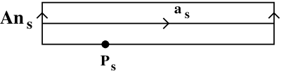
where $\approx$ is the relation defined as follows. Let $s,t\in S$ such that $m_{s\,t}=3$ and $s<t$. Put $p={\rm pos}(t:s)>0$ and $q={\rm pos}(s:t)<0$. For each $(x,y)\in[0,1]\times[0,1]$, the relation $\approx$ identifies the point $(2p+x,y)$ of ${\rm An}_{s}$ with the point $(2q+1-y,x)$ of ${\rm An}_{t}$ (see Figure 1). We identify each annulus ${\rm An}_{s}$ and the point $P_{s}$ with their image in $\Sigma$, respectively.

We now define the monodromy representation $\rho:A_{\Gamma}\to{\mathcal{M}}(\Sigma)$. Let $s\in S$, and put $k=|{\rm St}_{s}|$. We denote by $a_{s}:{\mathbb{S}}^{1}\to\Sigma$ the essential circle of $\Sigma$ such that $a_{s}(\theta)$ is the point $({k\theta\over\pi},{1\over 2})$ of ${\rm An}_{s}$ (see Figure 2). We let $\tau_{s}$ denote the Dehn twist along $a_{s}$. One has $a_{s}\cap a_{t}=\emptyset$ if $m_{s\,t}=2$, and $|a_{s}\cap a_{t}|=1$ if $m_{s\,t}=3$. Therefore, by Proposition 2.2, we have the following.

Proposition 2.3. Let $\Gamma$ be a small type Coxeter graph. There exists a well-defined group homomorphism $\rho:A_{\Gamma}\to{\mathcal{M}}(\Sigma)$ which sends $\sigma_{s}$ to $\tau_{s}$ for each $s\in S$.

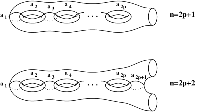
Example. Consider the braid group $B_{n}$, $n\geq 3$. If $n$ is odd, then the associated surface, $\Sigma$, is a surface of genus ${n-1\over 2}$ with one boundary component. If $n$ is even, then $\Sigma$ is a surface of genus ${n-2\over 2}$ with two boundary components (see Figure 3). For each $i=1,\dots,n-1$, let $a_{i}:{\mathbb{S}}^{1}\to\Sigma$ denote the essential circle pictured in Figure 3, and let $\tau_{i}$ denote the Dehn twist along $a_{i}$. Then the monodromy representation $\rho:B_{n}\to{\mathcal{M}}(\Sigma)$ of the braid group sends $\sigma_{i}$ to $\tau_{i}$ for all $i=1,\dots,n-1$.

Let ${\mathcal{O}}_{2}$ denote the ring of germs of functions at $0$ of ${\mathbb{C}}^{2}$. Let $f\in{\mathcal{O}}_{2}$ with an isolated singularity at $0$, and let $\mu$ be the Milnor number of $f$. To the germ $f$ one can associate a surface $\Sigma$ with boundary, called the Milnor fiber of $f$, an analytic subvariety ${\mathcal{D}}$ of ${\mathbb{D}}(\eta)=\{t\in{\mathbb{C}}^{\mu};\|t\|<\eta\}$, where $\eta>0$ is a small number, and a representation $\rho:\pi_{1}({\mathbb{D}}(\eta)\setminus{\mathcal{D}})\to{\mathcal{M}}(\Sigma)$, called the geometric monodromy of $f$. Recall that the simple singularities are defined by the equations

By [1] and [7], for each $\Gamma\in\{A_{n};n\geq 1\}\cup\{D_{n};n\geq 4\}\cup\{E_{6},E_{7},E_{8}\}$, the group $\pi_{1}({\mathbb{D}}(\eta)\setminus{\mathcal{D}})$ is isomorphic to the Artin group of type $\Gamma$, and $\rho:A_{\Gamma}\to{\mathcal{M}}(\Sigma)$ is the monodromy representation of the group $A_{\Gamma}$.

The monodromy representations are known to be faithful for $\Gamma=A_{n}$ and $\Gamma=D_{n}$ (see [45]), but are not faithful for $\Gamma\in\{E_{6},E_{7},E_{8}\}$ (see [51]). Actually, the monodromy representations are not faithful in general (see [36]).

Recall that the braid group $B_{n}$ has a presentation with generators $\sigma_{1},\dots,\sigma_{n-1}$ and relations

The submonoid generated by $\sigma_{1},\dots,\sigma_{n-1}$ is called the positive braid monoid on $n$ strings, and is denoted by $B_{n}^{+}$. It has a monoid presentation with generators $\sigma_{1},\dots,\sigma_{n-1}$ and relations (2) and (3), it is a Garside monoid, and the group of fractions of $B_{n}^{+}$ is $B_{n}$.

The starting point of the present section is the following result due to Dehornoy [13].

Theorem 3.1 (Dehornoy [13]). The Artin braid group $B_{n}$ is left-orderable, by an ordering which is a well-ordering when restricted to $B_{n}^{+}$.

Left-invariant orderings are important because of a long-standing conjecture in group theory: that the group ring of a torsion-free group has no zero divisors. This conjecture is true for left-orderable groups, thus Theorem 3.1 implies that ${\mathbb{Z}}[B_{n}]$ has no zero divisors. However, the main point of interest of Theorem 3.1 is not only the mere existence of orderings on the braid groups, but the particular nature of the construction. This has been already used to prove that some representations of the braid groups by automorphisms of groups are faithful (see [50] and [12]), and to study the so-called “weak faithfulness” of the Burau representation (see [14]), and I am sure that these ideas will be exploited again in the future.

Let $G$ be a left-orderable group, and let $<$ be a left invariant linear ordering on $G$. Call an element $g\in G$ positive if $g>1$, and denote by ${\mathcal{P}}$ the set of positive elements. Then ${\mathcal{P}}$ is a subsemigroup (i.e. ${\mathcal{P}}\cdot{\mathcal{P}}\subset{\mathcal{P}}$), and we have the disjoint union $G={\mathcal{P}}\sqcup{\mathcal{P}}^{-1}\sqcup\{1\}$, where ${\mathcal{P}}^{-1}=\{g^{-1};g\in{\mathcal{P}}\}$. Conversely, if ${\mathcal{P}}$ is a subsemigroup of $G$ such that $G={\mathcal{P}}\sqcup{\mathcal{P}}^{-1}\sqcup\{1\}$, then the relation $<$ defined by $f<g$ if $f^{-1}g\in{\mathcal{P}}$ is a left invariant linear ordering on $G$.

The description of the positive elements in Dehornoy’s ordering is based on the following result which, in my view, is more interesting than the mere existence of the ordering, because it leads to new techniques to study the braid groups.

Let $B_{n-1}$ be the subgroup of $B_{n}$ generated by $\sigma_{1},\dots,\sigma_{n-2}$. Let $\beta\in B_{n}$. We say that $\beta$ is $\sigma_{n-1}$-positive if it can be written

where $l\geq 1$ and $\alpha_{0},\alpha_{1},\dots,\alpha_{l}\in B_{n-1}$. We say that $\beta$ is $\sigma_{n-1}$-negative if it can be written

where $l\geq 1$ and $\alpha_{0},\alpha_{1},\dots,\alpha_{l}\in B_{n-1}$. We denote by ${\mathcal{P}}_{n-1}$ the set of $\sigma_{n-1}$-positive elements, and by ${\mathcal{P}}_{n-1}^{-}$ the set of $\sigma_{n-1}$-negative elements. Note that ${\mathcal{P}}_{n-1}^{-}={\mathcal{P}}_{n-1}^{-1}=\{\beta^{-1};\beta\in{\mathcal{P}}_{n-1}\}$.

Theorem 3.2 (Dehornoy [13]). We have the disjoint union $B_{n}={\mathcal{P}}_{n-1}\sqcup{\mathcal{P}}_{n-1}^{-}\sqcup B_{n-1}$.

Now, the set ${\mathcal{P}}$ of positive elements in Dehornoy’s ordering can be described as follows. For $k=1,\dots,n-1$, let ${\mathcal{P}}_{k}$ denote the set of $\sigma_{k}$-positive elements in $B_{k+1}$, where $B_{k+1}$ is viewed as the subgroup of $B_{n}$ generated by $\sigma_{1},\dots,\sigma_{k}$. Then ${\mathcal{P}}={\mathcal{P}}_{1}\sqcup{\mathcal{P}}_{2}\sqcup\dots\sqcup{\mathcal{P}}_{n-1}$. It is easily checked using Theorem 3.2 that ${\mathcal{P}}$ is a subsemigroup of $B_{n}$ and that $B_{n}={\mathcal{P}}\sqcup{\mathcal{P}}^{-1}\sqcup\{1\}$.

Dehornoy’s proof of Theorem 3.2 involves rather delicate combinatorial and algebraic constructions which were partly motivated by questions in set theory. A topological construction of Dehornoy’s ordering of the braid group $B_{n}$, viewed as the mapping class group of the $n$-punctured disk, is given in [24]. This last construction has been extended to the mapping class groups of the punctured surfaces with non-empty boundary by Rourke and Wiest [48]. This extension involves some choices, and, therefore, is not canonical. However, it is strongly connected to Mosher’s normal forms [42] and, as with Dehornoy’s ordering, is sufficiently explicit to be used for other purposes (to study faithfulness properties of “some” representations of the mapping class group, for example. This is just an idea…). Another approach (see [49]) based on Nielsen’s ideas [43] gives rise to many other linear orderings of the braid groups, and, more generally, of the mapping class groups of punctured surfaces with non-empty boundary, but I am not convinced that these orderings are explicit enough to be used for other purposes.

The mapping class group of a (punctured) closed surface is definitively not left-orderable because it has torsion. However, it is an open question to determine whether some special torsion-free subgroups of ${\mathcal{M}}(\Sigma)$ such as Ivanov’s group $\Gamma_{m}(\Sigma)$ (see [32]) are orderable. The Torelli group is residually torsion-free nilpotent (see [27]), therefore is biorderable. We refer to [17] for a detailed account on Dehornoy’s ordering and related questions.

Let $f\in{\mathcal{M}}(\Sigma,{\mathcal{P}})$. We say that $f$ is a pseudo-Anosov element if it has no finite orbit in ${\mathcal{C}}(\Sigma,{\mathcal{P}})$, we say that $f$ is periodic if $f^{m}$ acts trivially on ${\mathcal{C}}(\Sigma,{\mathcal{P}})$ for some $m\geq 1$, and we say that $f$ is reducible otherwise.

The use of the action of ${\mathcal{M}}(\Sigma,{\mathcal{P}})$ on ${\mathcal{C}}(\Sigma,{\mathcal{P}})$ and the “Thurston classification” of the elements of ${\mathcal{M}}(\Sigma,{\mathcal{P}})$ play a prominent role in the study of the algebraic properties of the mapping class groups. Here are some applications.

Theorem 4.1.

1. 1.

   (Ivanov [32]). Let $f$ be a pseudo-Anosov element of ${\mathcal{M}}(\Sigma,{\mathcal{P}})$. Then $f$ has infinite order, $\langle f\rangle\cap Z({\mathcal{M}}(\Sigma,{\mathcal{P}}))=\{1\}$, where $\langle f\rangle$ denotes the subgroup generated by $f$, and $\langle f\rangle\times Z({\mathcal{M}}(\Sigma,{\mathcal{P}}))$ is a subgroup of finite index of the centralizer of $f$ in ${\mathcal{M}}(\Sigma,{\mathcal{P}})$.

2. 2.

   (Birman, Lubotzky, McCarthy [5]). If a subgroup of ${\mathcal{M}}(\Sigma,{\mathcal{P}})$ contains a solvable subgroup of finite index, then it contains an abelian subgroup of finite index.

3. 3.

   (Ivanov [32], McCarthy [40]). Let $G$ be a subgroup of ${\mathcal{M}}(\Sigma,{\mathcal{P}})$. Then either $G$ contains a free group of rank 2, or $G$ contains an abelian subgroup of finite index.

The use of the action of ${\mathcal{M}}(\Sigma,{\mathcal{P}})$ on ${\mathcal{C}}(\Sigma,{\mathcal{P}})$ is also essential in the determination of the (maximal) free abelian subgroups of ${\mathcal{M}}(\Sigma,{\mathcal{P}})$ (see [5]), and in the calculation of the automorphism group and abstract commensurator group of ${\mathcal{M}}(\Sigma,{\mathcal{P}})$ (see [31], [33], [41], [34]).

The present section concerns the question of how to translate these techniques to other groups such as the (spherical type) Artin groups, or the Coxeter groups.

Let $\Gamma$ be a Coxeter graph, let $M=(m_{s\,t})_{s,t\in S}$ be the Coxeter matrix of $\Gamma$, and let $A=A_{\Gamma}$ be the Artin group of type $\Gamma$. For $X\subset S$, we denote by $\Gamma_{X}$ the full subgraph of $\Gamma$ generated by $X$, and by $A_{X}$ the subgroup of $A$ generated by ${\mathcal{S}}_{X}=\{\sigma_{x};x\in X\}$. By [38] (see also [44]), the group $A_{X}$ is the Artin group of type $\Gamma_{X}$. A subgroup of the form $A_{X}$ is called a standard parabolic subgroup, and a subgroup which is conjugate to a standard parabolic subgroup is simply called a parabolic subgroup. We shall denote by ${\mathcal{A}}{\mathcal{C}}={\mathcal{A}}{\mathcal{C}}(\Gamma)$ the set of parabolic subgroups different from $A$ and from $\{1\}$.

Let $f\in A$. We say that $f$ is an (algebraic) pseudo-Anosov element if it has no finite orbit in ${\mathcal{A}}{\mathcal{C}}$, we say that $f$ is an (algebraic) periodic element if $f^{m}$ acts trivially on ${\mathcal{A}}{\mathcal{C}}$ for some $m>0$, and we say that $f$ is an (algebraic) reducible element otherwise.

The above definitions are motivated by the following result.

Proposition 4.2. Let $f$ be an element of the braid group $B_{n}$ (viewed as the mapping class group ${\mathcal{M}}({\mathbb{D}},{\mathcal{P}})$ as well as the Artin group associated to the Dynkin graph $A_{n-1}$).

• •

  $f$ is a pseudo-Anosov element if and only if $f$ is an algebraic pseudo-Anosov element.

• •

  $f$ is a periodic element if and only if $f$ is an algebraic periodic element.

• •

  $f$ is a reducible element if and only if $f$ is an algebraic reducible element.

Proof. Recall that ${\mathbb{D}}=\{z\in{\mathbb{C}};|z|\leq 1\}$, ${\mathcal{P}}=\{P_{1},\dots,P_{n}\}$ is a set of $n$ punctures in the interior of ${\mathbb{D}}$, and $B_{n}={\mathcal{M}}({\mathbb{D}},{\mathcal{P}})$. Let $\sigma_{1},\dots,\sigma_{n-1}$ be the standard generators of $B_{n}$. We can assume that each $\sigma_{i}$ acts trivially outside a disk containing $P_{i}$ and $P_{i+1}$, and permutes $P_{i}$ and $P_{i+1}$.

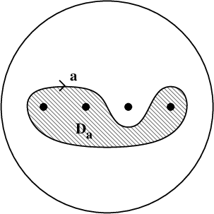
Let $a:{\mathbb{S}}^{1}\to{\mathbb{D}}\setminus{\mathcal{P}}$ be a generic circle. Then $a({\mathbb{S}}^{1})$ separates ${\mathbb{D}}$ into two components: a disk ${\mathbb{D}}_{a}$ bounded by $a({\mathbb{S}}^{1})$, and an annulus ${\mathbb{A}}_{a}$ bounded by $a({\mathbb{S}}^{1})\sqcup{\mathbb{S}}^{1}$, where ${\mathbb{S}}^{1}=\{z\in{\mathbb{C}};|z|=1\}$ (see Figure 4). Let $m=|{\mathbb{D}}_{a}\cap{\mathcal{P}}|$. Then the hypothesis “$a$ is generic” implies that $2\leq m\leq n-1$. Furthermore, the group ${\mathcal{M}}({\mathbb{D}}_{a},{\mathbb{D}}_{a}\cap{\mathcal{P}})$ is isomorphic to $B_{m}$.

Let $\tau_{a}$ denote the Dehn twist along $a$. If $m=|{\mathbb{D}}_{a}\cap{\mathcal{P}}|\geq 3$, then the center $Z({\mathcal{M}}({\mathbb{D}}_{a},{\mathbb{D}}_{a}\cap{\mathcal{P}}))$ of ${\mathcal{M}}({\mathbb{D}}_{a},{\mathbb{D}}_{a}\cap{\mathcal{P}})$ is the (infinite) cyclic subgroup generated by $\tau_{a}$. If $m=2$, then ${\mathcal{M}}({\mathbb{D}}_{a},{\mathbb{D}}_{a}\cap{\mathcal{P}})$ is an infinite cyclic group, and $\tau_{a}$ generates the (unique) index 2 subgroup of ${\mathcal{M}}({\mathbb{D}}_{a},{\mathbb{D}}_{a}\cap{\mathcal{P}})$. Recall that, if $\tau_{a_{1}}$ and $\tau_{a_{2}}$ are two Dehn twists along generic circles $a_{1}$ and $a_{2}$, respectively, and if $\tau_{a_{1}}^{k_{1}}=\tau_{a_{2}}^{k_{2}}$ for some $k_{1},k_{2}\in{\mathbb{Z}}\setminus\{0\}$, then $k_{1}=k_{2}$ and $a_{1}=a_{2}$. Recall also that, if $\tau_{a}$ is the Dehn twist along a generic circle $a$, then $g\tau_{a}g^{-1}$ is the Dehn twist along $g(a)$, for any $g\in{\mathcal{M}}({\mathbb{D}},{\mathcal{P}})$. We conclude from the above observations that, if $g\cdot{\mathcal{M}}({\mathbb{D}}_{a},{\mathbb{D}}_{a}\cap{\mathcal{P}})\cdot g^{-1}={\mathcal{M}}({\mathbb{D}}_{a},{\mathbb{D}}_{a}\cap{\mathcal{P}})$, then $g(a)=a$. Conversely, if $g(a)=a$, then $g({\mathbb{D}}_{a},{\mathbb{D}}_{a}\cap{\mathcal{P}})=({\mathbb{D}}_{a},{\mathbb{D}}_{a}\cap{\mathcal{P}})$, thus $g\cdot{\mathcal{M}}({\mathbb{D}}_{a},{\mathbb{D}}_{a}\cap{\mathcal{P}})\cdot g^{-1}={\mathcal{M}}({\mathbb{D}}_{a},{\mathbb{D}}_{a}\cap{\mathcal{P}})$.

Write $S=\{1,2,\dots,n-1\}$. For $X\subset S$, we set ${\mathcal{S}}_{X}=\{\sigma_{x};x\in X\}$, and denote by $(B_{n})_{X}$ the subgroup of $B_{n}$ generated by ${\mathcal{S}}_{X}$.

Let $1\leq m\leq n-2$, and $X(m)=\{1,2,\dots,m\}$. We can choose a generic circle $a_{m}:{\mathbb{S}}^{1}\to{\mathbb{D}}\setminus{\mathcal{P}}$ such that ${\mathbb{D}}_{a_{m}}\cap{\mathcal{P}}=\{P_{1},\dots,P_{m},P_{m+1}\}$ and ${\mathcal{M}}({\mathbb{D}}_{a_{m}},{\mathbb{D}}_{a_{m}}\cap{\mathcal{P}})=(B_{n})_{X(m)}$ (see Figure 5). Observe that, if $a:{\mathbb{S}}^{1}\to{\mathbb{D}}\setminus{\mathcal{P}}$ is a generic circle such that $|{\mathbb{D}}_{a}\cap{\mathcal{P}}|=m+1$, then there exists $g\in{\mathcal{M}}({\mathbb{D}},{\mathcal{P}})=B_{n}$ such that $g{\mathcal{M}}({\mathbb{D}}_{a},{\mathbb{D}}_{a}\cap{\mathcal{P}})g^{-1}={\mathcal{M}}({\mathbb{D}}_{a_{m}},{\mathbb{D}}_{a_{m}}\cap{\mathcal{P}})=(B_{n})_{X(m)}$. In particular, ${\mathcal{M}}({\mathbb{D}}_{a},{\mathbb{D}}_{a}\cap{\mathcal{P}})$ is a parabolic subgroup of $B_{n}$.

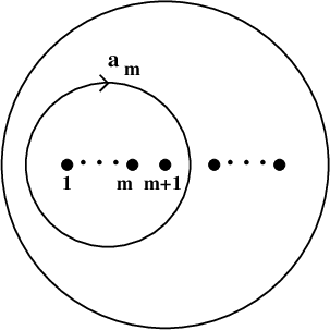
Take $X\subset S$, $X\neq S$. Decompose $X$ as a disjoint union $X=X_{1}\sqcup X_{2}\sqcup\dots\sqcup X_{q}$, where $X_{k}=\{i_{k},i_{k}+1,\dots,i_{k}+t_{k}\}$ for some $i_{k}\in\{1,\dots,n-1\}$ and some $t_{k}\in{\mathbb{N}}$, and $i_{k}+t_{k}+1<i_{k+1}$, for all $k=1,\dots,q$. We can choose generic circles $b_{1},\dots,b_{q}:{\mathbb{S}}^{1}\to{\mathbb{D}}\setminus{\mathcal{P}}$ such that

(See Figure 6.) It is easily checked that

and the only Dehn twists which lie in the center of $(B_{n})_{X}$ are $\tau_{b_{1}},\tau_{b_{2}},\dots,\tau_{b_{q}}$.

Let $g\in{\mathcal{M}}({\mathbb{D}},{\mathcal{P}})$ which fixes some $a\in{\mathcal{C}}({\mathbb{D}},{\mathcal{P}})$. Then $g{\mathcal{M}}({\mathbb{D}}_{a},{\mathbb{D}}_{a}\cap{\mathcal{P}})g^{-1}={\mathcal{M}}({\mathbb{D}}_{a},{\mathbb{D}}_{a}\cap{\mathcal{P}})$ and ${\mathcal{M}}({\mathbb{D}}_{a},{\mathbb{D}}_{a}\cap{\mathcal{P}})$ is a parabolic subgroup, thus $g$ fixes some element in ${\mathcal{A}}{\mathcal{C}}$.

Let $g\in{\mathcal{M}}({\mathbb{D}},{\mathcal{P}})$ which fixes some element in ${\mathcal{A}}{\mathcal{C}}$. Up to conjugation, we may suppose that there exists $X\subset S$ such that $g(B_{n})_{X}g^{-1}=(B_{n})_{X}$. We take again the notations introduced above. Recall that the only Dehn twists which lie in the center of $(B_{n})_{X}$ are $\tau_{b_{1}},\tau_{b_{2}},\dots,\tau_{b_{q}}$, thus $g$ must permute the set $\{\tau_{b_{1}},\tau_{b_{2}},\dots,\tau_{b_{q}}\}$. So, there exists $m\geq 1$ such that $g^{m}\tau_{b_{1}}g^{-m}=\tau_{b_{1}}$, that is, $g^{m}(b_{1})=b_{1}$.

Let $g\in{\mathcal{M}}({\mathbb{D}},{\mathcal{P}})$ which fixes all the elements of ${\mathcal{C}}({\mathbb{D}},{\mathcal{P}})$. Let $A\in{\mathcal{A}}{\mathcal{C}}$. There exist $h\in B_{n}$ and $X\subset S$ such that $A=h(B_{n})_{X}h^{-1}$. We keep the notations used above. The element $h^{-1}gh$ also fixes all the elements of ${\mathcal{C}}({\mathbb{D}},{\mathcal{P}})$. In particular, we have $(h^{-1}gh)(b_{k})=b_{k}$ for all $k=1,\dots,q$. This implies that $h^{-1}gh$ fixes ${\mathcal{M}}({\mathbb{D}}_{b_{k}},{\mathbb{D}}_{b_{k}}\cap{\mathcal{P}})$ for all $k=1,\dots,q$, thus $h^{-1}gh$ fixes $(B_{n})_{X}={\mathcal{M}}({\mathbb{D}}_{b_{1}},{\mathbb{D}}_{b_{1}}\cap{\mathcal{P}})\times\dots\times{\mathcal{M}}({\mathbb{D}}_{b_{q}},{\mathbb{D}}_{b_{q}}\cap{\mathcal{P}})$, therefore $g$ fixes $A=h(B_{n})_{X}h^{-1}$.

References

- [1] V.I. Arnold, Normal forms of functions near degenerate critical points, the Weyl groups , , and Lagrangian singularities, Funkcional. Anal. i Prilov zen. 6 (1972), no. 4, 3–25.
- [2] D. Bessis, R. Corran, Garside structure for the braid group of , preprint.
- [3] J.S. Birman, Braids, links, and mapping class groups, Annals of Mathematics Studies, No. 82, Princeton University Press, Princeton, N.J., 1974.
- [4] J.S. Birman, Mapping class groups of surfaces, Braids (Santa Cruz, CA, 1986), 13–43, Contemp. Math., 78, Amer. Math. Soc., Providence, RI, 1988.
- [5] J.S. Birman, A. Lubotzky, J. McCarthy, Abelian and solvable subgroups of the mapping class groups, Duke Math. J. 50 (1983), 1107–1120.
- [6] N. Bourbaki, Groupes et algèbres de Lie, chapitres 4, 5 et 6, Hermann, Paris, 1968.
- [7] E. Brieskorn, Die Fundamentalgruppe des Raumes der regulären Orbits einer endlichen komplexen Spiegelungsgruppe, Invent. Math. 12 (1971), 57–61.
- [8] E. Brieskorn, K. Saito, Artin-Gruppen und Coxeter-Gruppen, Invent. Math. 17 (1972), 245–271.
- [9] R. Charney, M.W. Davis, The -problem for hyperplane complements associated to infinite reflection groups, J. Amer. Math. Soc. 8 (1995), 597–627.
- [10] R. Charney, J. Meier, K. Whittlesey, Bestvina’s normal form complex and the homology of Garside groups, Geom. Dedicata 105 (2004), 171–188.
- [11] J. Crisp, L. Paris, The solution to a conjecture of Tits on the subgroup generated by the squares of the generators of an Artrin group, Invent. Math. 145 (2001), 19–36.
- [12] J. Crisp, L. Paris, Representations of the braid group by automorphisms of groups, invariants of links, and Garside groups, Pacific J. Math., to appear.
- [13] P. Dehornoy, Braid groups and left distributive operations, Trans. Amer. Math. Soc. 343 (1994), 115–150.
- [14] P. Dehornoy, Weak faithfulness properties for the Burau representation, Topology Appl. 69 (1996), 121–143.
- [15] P. Dehornoy, Gaussian groups are torsion free, J. Algebra 210 (1998), 291–297.
- [16] P. Dehornoy, Groupes de Garside, Ann. Sci. Ecole Norm. Sup. (4) 35 (2002), 267–306.
- [17] P. Dehornoy, I. Dynnikov, D. Rolfsen, B. Wiest, Why are braids orderable? Panoramas et Synthèses, 14, Société Mathématique de France, Paris, 2002.
- [18] P. Dehornoy, Y. Lafont, Homology of Gaussian groups, Ann. Inst. Fourier (Grenoble) 53 (2003), 489–540.
- [19] P. Dehornoy, L. Paris, Gaussian groups and Garside groups, two generalisations of Artin groups, Proc. London Math. Soc. (3) 79 (1999), 569–604.
- [20] P. Deligne, Les immeubles des groupes de tresses généralisés, Invent. Math. 17 (1972), 273–302.
- [21] G. Duchamp, D. Krob, The lower central series of the free partially commutative group, Semigroup Forum 45 (1992), 385–394.
- [22] D.B.A. Epstein, J.W. Cannon, D.F. Holt, S.V.F. Levy, M.S. Paterson, W.P. Thurston, Word processing in groups, Jones and Bartlett Publishers, Boston, MA, 1992.
- [23] E. Fadell, L. Neuwirth, Configuration spaces, Math. Scand. 10 (1962), 111–118.
- [24] R. Fenn, M.T. Greene, D. Rolfsen, C. Rourke, B. Wiest, Ordering the braid groups, Pacific J. Math. 191 (1999), 49–74.
- [25] N. Franco, J. González-Meneses, Conjugacy problem for braid groups and Garside groups, J. Algebra 266 (2003), 112–132.
- [26] F.A. Garside, The braid group and other groups, Quart. J. Math. Oxford Ser. (2) 20 (1969), 235–254.
- [27] R. Hain, Infinitesimal presentations of the Torelli groups, J. Amer. Math. Soc. 10 (1997), no. 3, 597–651.
- [28] E. Godelle, Normalisateur et groupe d’Artin de type sphérique, J. Algebra 269 (2003), 263–274.
- [29] H. Hiller, Geometry of Coxeter groups, Research Notes in Mathematics, 54, Pitman (Advanced Publishing Program), Boston, Mass.–London, 1982.
- [30] J.E. Humphreys, Reflection groups and Coxeter groups, Cambridge Studies in Advanced Mathematics, 29, Cambridge University Press, Cambridge, 1990.
- [31] N.V. Ivanov, Automorphisms of Teichmüller modular groups, Topology and geometry - Rohlin Seminar, 199–270, Lecture Notes in Math., 1346, Springer, Berlin, 1988.
- [32] N.V. Ivanov, Subgroups of Teichmüller modular groups, Translations of Mathematical Monographs, 115, American Mathematical Society, Providence, RI, 1992.
- [33] N.V. Ivanov, Automorphism of complexes of curves and of Teichmüller spaces, Internat. Math. Res. Notices 14 (1997), 651–666.
- [34] N.V. Ivanov, J.D. McCarthy, On injective homomorphisms between Teichmüller modular groups. I, Invent. Math. 135 (1999), 425–486.
- [35] D. Krammer, The conjugacy problem for Coxeter groups, Ph. D. Thesis, Universiteit Utrecht, 1995.
- [36] C. Labruère, Generalized braid groups and mapping class groups, J. Knot Theory Ramifications 6 (1997), 715–726.
- [37] C. Labruère, L. Paris, Presentations for the punctured mapping class groups in terms of Artin groups, Algebr. Geom. Topol. 1 (2001), 73–114.
- [38] H. Van der Lek, The homotopy type of complex hyperplane complements, Ph. D. Thesis, Nijmegen, 1983.
- [39] M. Matsumoto, A presentation of mapping class groups in terms of Artin groups and geometric monodromy of singularities, Math. Ann. 316 (2000), 401–418.
- [40] J. McCarthy, A “Tits-alternative” for subgroups of surface mapping class groups, Trans. Amer. Math. Soc. 291 (1985), 583–612.
- [41] J. McCarthy, Automorphisms of surface mapping class groups. A recent theorem of N. Ivanov, Invent. Math. 84 (1986), 49–71.
- [42] L. Mosher, Mapping class groups are automatic, Ann. of Math. (2) 142 (1995), 303–384.
- [43] J. Nielsen, Untersuchungen zur Topologie des geschlossenen zweiseitigen Flächen, Acta Math. 50 (1927), 189–358.
- [44] L. Paris, Parabolic subgroups of Artin groups, J. Algebra 196 (1997), 369–399.
- [45] B. Perron, J.P. Vannier, Groupe de monodromie géométrique des singularités simples, Math. Ann. 306 (1996), 231–245.
- [46] M. Picantin, The conjugacy problem in small Gaussian groups, Comm. Algebra 29 (2001), 1021–1039.
- [47] M. Picantin, Automatic structures for torus link groups, J. Knot Theory Ramifications 12 (2003), 833–866.
- [48] C. Rourke, B. Wiest, Order automatic mapping class groups, Pacific J. Math. 194 (2000), 209–227.
- [49] H. Short, B. Wiest, Orderings of mapping class groups after Thurston, Enseign. Math. (2) 46 (2000), 279–312.
- [50] V. Shpilrain, Representing braids by automorphisms, Internat. J. Algebra Comput. 11 (2001), 773–777.
- [51] B. Wajnryb, Artin groups and geometric monodromy, Invent. Math. 138 (1999), 563–571.
Luis Paris,
Institut de Mathématiques de Bourgogne, UMR 5584 du CNRS, Université de Bourgogne, B.P. 47870, 21078 Dijon cedex, France
E-mail: lparis@u-bourgogne.fr