Weak Forms of the Ehrenpreis Conjecture and the Surface Subgroup Conjecture

Lewis Bowen Note: Research supported in part by a Max Zorn Postdoctoral Fellowship

Abstract

We prove the following:

1.

Let $\epsilon>0$ and let $S_{1},S_{2}$ be two closed hyperbolic surfaces. Then there exists locally-isometric covers ${\tilde{S}_{i}}$ of $S_{i}$ (for $i=1,2$ ) such that there is a $(1+\epsilon)$ bi-Lipschitz homeomorphism between ${\tilde{S}_{1}}$ and ${\tilde{S}_{2}}$ and both covers ${\tilde{S}_{i}}$ ( $i=1,2$ ) have bounded injectivity radius.
2.

Let ${\cal M}$ be a closed hyperbolic $3$ -manifold. Then there exists a map $j:S\to{\cal M}$ where $S$ is a surface of bounded injectivity radius and $j$ is $\pi_{1}$ -injective local isometry onto its image.

MSC: 20E07, 57M10, 57M50
Keywords: Ehrenpreis conjecture, surface subgroup, hyperbolic groups.

1 Introduction

1.1 The Ehrenpreis Conjecture

Conjecture 1.1.

(The Ehrenpreis Conjecture) Let $\epsilon>0$ and let $S_{1},S_{2}$ be two closed Riemann surfaces of the same genus. Then there exists finite-sheeted conformal covers ${\tilde{S}_{i}}$ of $S_{i}$ (for $i=1,2$ ) such that there is a $(1+\epsilon)$ -quasiconformal homeomorphism between ${\tilde{S}_{1}}$ and ${\tilde{S}_{2}}$ .

The Ehrenpreis conjecture was introduced in [Ehrenpreis] where it was proven in the case that $S_{1}$ and $S_{2}$ are tori. In the appendix to [Gendron] it is shown that in the remaining cases the conjecture is equivalent to the following.

Conjecture 1.2.

(The hyperbolic Ehrenpreis conjecture) Let $\epsilon>0$ and let $S_{1},S_{2}$ be two closed hyperbolic surfaces. Then there exists finite-sheeted locally isometric covers ${\tilde{S}_{i}}$ of $S_{i}$ (for $i=1,2$ ) such that there is a $(1+\epsilon)$ bi-Lipschitz homeomorphism between ${\tilde{S}_{1}}$ and ${\tilde{S}_{2}}$ .

As a corollary to our first main theorem we will prove the above conjecture with “finite-sheeted” replaced by “bounded injectivity radius”. We need some terminology. A pair of pants $H$ is a surface homeomorphic to the $2-$ sphere minus three open disks. It is boundary-ordered if the boundary components are ordered, in which case we may refer to the first boundary component of $H$ by $\partial_{1}H$ , the second by $\partial_{2}H$ and so on. A labeled pants decomposition of a surface $S$ is a collection ${\cal P}$ of boundary-ordered pants embedded in $S$ whose interiors are pairwise-disjoint and whose union is all of $S$ . We also require that “labels” match: if $\gamma$ is a simple closed curve in $S$ and $\gamma$ is in the boundary of $H_{1},H_{2}\in{\cal P}$ then we require $\gamma=\partial_{i}H_{1}=\partial_{i}H_{2}$ for some $i\in\{1,2,3\}$ . Let ${\cal P}^{*}=\{\partial_{i}H:\,i=1,2,3$ and $H\in{\cal P}\}$ . We require every curve in ${\cal P}^{*}$ to be oriented (but no restrictions are put on the orientations).

Theorem 1.3.

(Main theorem: Ehrenpreis case) Let $S_{1},S_{2}$ be two closed hyperbolic surfaces and let $\epsilon>0$ be given. Suppose that $S_{1}$ and $S_{2}$ are incommensurable. Then there exists an $L_{0}>0$ such that for all $L>L_{0}$ there exists locally isometric covers $\pi_{i}:{\tilde{S}_{i}}\to S_{i}$ (for $i=1,2$ ) such that for $i=1,2$ , ${\tilde{S}_{i}}$ has a labeled pants decomposition ${\cal P}_{i}$ and there is a homeomorphism $h:{\tilde{S}_{1}}\to{\tilde{S}_{2}}$ such that $h({\cal P}_{1})={\cal P}_{2}$ , $h({\cal P}^{*}_{1})={\cal P}^{*}_{2}$ and for every curve $\gamma\in{\cal P}_{1}^{*}$ ,

$\displaystyle\|length(\gamma)-L\|$	$\displaystyle\leq$	$\displaystyle\epsilon,$
$\displaystyle\|length(h(\gamma))-L\|$	$\displaystyle\leq$	$\displaystyle\epsilon,$
$\displaystyle\|twist(\gamma)\|$	$\displaystyle\leq$	$\displaystyle{\hat{T}}\exp(-L/4),$
$\displaystyle\|twist(h(\gamma))\|$	$\displaystyle\leq$	$\displaystyle{\hat{T}}\exp(-L/4)\textrm{ and }$
$\displaystyle\|twist(\gamma)-twist(h(\gamma))\|$	$\displaystyle\leq$	$\displaystyle\epsilon\exp(-L/4).$

Here ${\hat{T}}$ is a constant that depends only on $S_{1},S_{2}$ and $\epsilon$ .

For the definition of $twist(\gamma)$ , see section 6.

Remark 1.4.

The covers ${\tilde{S}_{i}}$ constructed to prove this theorem are analytically infinite, genus 0 and without boundary. However, they have bounded injectivity radius.

Remark 1.5.

The significance of the number $\exp(-L/4)$ lies in the fact that if $P$ is a hyperbolic pair of pants with geodesic boundary in which all boundary components have length $L$ then the distance between any two distinct boundary components is $2\exp(-L/4)+O(\exp(-3L/4))$ .

We also prove:

Theorem 1.6.

Let $\epsilon_{0}>0$ . Then there exists an $\epsilon,L_{1}>0$ such that if two surfaces ${\tilde{S}_{i}}$ ( $i=1,2$ ) satisfy the conclusion of theorem 1.3 with $L>L_{1}$ then there is a $(1+\epsilon_{0})$ bi-Lipschitz homeomorphism $h:{\tilde{S}_{1}}\to{\tilde{S}_{2}}$ .

The above two theorems imply the following weak form of the Ehrenpreis conjecture:

Theorem 1.7.

Let $\epsilon>0$ and let $S_{1},S_{2}$ be two closed hyperbolic surfaces. Then there exists locally isometric covers ${\tilde{S}_{i}}$ of $S_{i}$ (for $i=1,2$ ) such that

•

there is a $(1+\epsilon)$ bi-Lipschitz homeomorphism between ${\tilde{S}_{1}}$ and ${\tilde{S}_{2}}$ and
•

${\tilde{S}_{1}}$ , ${\tilde{S}_{2}}$ have bounded injectivity radius.

Question 1.8.

Can the conclusions to theorem 1.3 be strengthened so that ${\tilde{S}_{i}}$ is closed?

We will show (in part III) that given $L,\epsilon,S_{1},S_{2}$ the above question is equivalent to a linear programming problem. We intend to study this problem in more detail in a future paper.

1.2 The Surface Subgroup Conjecture

Conjecture 1.9.

(The Surface Subgroup Conjecture) Let ${\cal M}$ be a closed hyperbolic $3$ -manifold. Then there exists a $\pi_{1}$ -injective map $j:S\to{\cal M}$ from a closed surface $S$ of genus at least 2 into ${\cal M}$ .

Perhaps the original motivation for the surface subgroup conjecture is its relationship to the Virtual Haken Conjecture. The latter states that every irreducible closed $3$ -manifold ${\cal M}$ with infinite fundamental group has a finite sheeted cover which contains an embedded incompressible closed surface. It was first stated in [Waldhausen]. The surface subgroup conjecture is an immediate consequence of the Virtual Haken conjecture and one may hope that it is a stepping stone towards the Virtual Haken conjecture.

We will prove the following main theorem.

Theorem 1.10.

(Main theorem: surface subgroup case) Let ${\cal M}$ be a closed hyperbolic $3$ -manifold. Suppose that ${\cal M}$ does not contain a closed totally geodesic immersed surface. Let $\epsilon>0$ be given. Then there exists an $L_{0}$ such that for all $L>L_{0}$ the following holds. There exists a map $j:S\to{\cal M}$ from a surface $S$ that has a labeled pants decomposition ${\cal P}$ such that for every curve $\gamma\in{\cal P}^{*}$

$\displaystyle\|length_{j}(\gamma)-L\|$	$\displaystyle\leq$	$\displaystyle\epsilon,$
$\displaystyle\|twist(\gamma)\|$	$\displaystyle\leq$	$\displaystyle{\hat{T}}\exp(-L/4)\textrm{ and }$
$\displaystyle\|\Im(twist_{j}(\gamma))\|$	$\displaystyle\leq$	$\displaystyle\epsilon\exp(-L/4).$

Here ${\hat{T}}$ is a constant depending only on ${\cal M}$ and $\epsilon$ . $length(\gamma)$ and $twist(\gamma)$ denote the complex length and complex twist parameter of $\gamma$ with respect to $j$ (see section 6).

We will also prove:

Theorem 1.11.

There exist positive numbers $\epsilon_{0},L_{1}>0$ such that for any $0<\epsilon<\epsilon_{0}$ and $L>L_{1}$ if $j:S\to{\cal M}$ is a map from a surface into a hyperbolic $3$ -manifold ${\cal M}$ satisfying the conclusion of theorem 1.10 then $j$ is $\pi_{1}$ -injective.

Question 1.12.

Can the surface $S$ in theorem 1.10 be chosen to be closed?

An affirmative answer would imply the surface subgroup conjecture. We will show (in part III) that given $L,\epsilon,{\cal M}$ the above question is equivalent to a linear programming problem.

1.3 A word on the proof and organization of the paper

The proof of the main theorems rely on what we call the isometry construction. It is a method for perturbing a given isometry into a given discrete group using the horocyclic flow. It is sketched in section 8. In part II, bounds on the translation distance and position of the perturbed isometry are proven. These bounds are then used to prove the main theorems in section 10. In part III, it shown that any specific instance of questions 1.8 and 1.12 is equivalent to a certain linear programming problem. We are, as of yet, unable to show that the linear programming has a solution; though we can show (unpublished) that the corresponding system of linear equations has a solution space of relatively small codimension.

The proofs of theorems 1.6 and 1.11 are handled in parts IV and V respectively.

Acknowledgements: We would like to thank Joel Hass for many encouraging conversations.

Part I Background and Notation

2 Estimate Notation

In this paper, we will have several variables $T,\epsilon,\delta$ , etc. However the variable $L$ will be treated in a special way. If $f$ is a function of $L$ and $x$ is a quantity that may depend on several variables (including $L$ ) then the notation $x=O(f(L))$ means there exist positive constants $k,L_{0}$ that do not depend on $L$ but may depend on other variables such that for all $L>L_{0}$

|x|\leq kf(L).

If $x=y+O(f(L))$ and $z=w+O(g(L))$ and if $f(L)/y\to 0$ as $L\to\infty$ and $g(L)/w\to 0$ as $L\to\infty$ then

\frac{x}{z}-\frac{y}{w}=O(f(L)/w+yg(L)/w^{2}).

We use the following to express the above:

\displaystyle\frac{x}{z}=\frac{y+O(f(L))}{w+O(g(L))}=\frac{y}{w}+O(f(L)/w+yg(L)/w^{2})

We will write $f(L)\sim g(L)$ to mean

\lim_{L\to\infty}\,\frac{f(L)}{g(L)}=1.

We will write $f(L)\approx g(L)$ to mean that there exist positive constants $k_{1},k_{2},L_{0}$ such that for all $L>L_{0}$

k_{1}f(L)\leq g(L)\leq k_{2}f(L).

3 Groups of isometries of Hyperbolic Space

Throughout this paper (unless explicitly stated otherwise), we will use the upperhalf space model of $3$ -dimensional hyperbolic space which we denote by ${\mathbb{H}}^{3}$ . In this model,

{\mathbb{H}}^{3}=\{(z,t):z\in{\mathbb{C}},t>0\}

is equipped with the metric $ds^{2}=(|dz|^{2}+dt^{2})/t^{2}$ . See, for example [Ratcliffe] or [Fenchel] for more details.

The hyperbolic plane ${\mathbb{H}}^{2}=\{(x,t):x\in{\mathbb{R}},t>0\}\subset{\mathbb{H}}^{3}$ is isometrically embedded in ${\mathbb{H}}^{3}$ . We identify the group of orientation-preserving isometries of ${\mathbb{H}}^{3}$ with $PSL_{2}({\mathbb{C}})$ . $PSL_{2}({\mathbb{C}})$ acts on the complex plane ${\mathbb{C}}\times\{0\}\subset{\mathbb{C}}\times[0,\infty)$ by fractional linear transformations as follows:

\left[\begin{array}[]{cc}a&b\\ c&d\end{array}\right]z=\frac{az+b}{cz+d}.

The action of $PSL_{2}({\mathbb{C}})$ on ${\mathbb{H}}^{3}$ is defined by extending the above action to ${\mathbb{H}}^{3}$ via the rule that for every $A\in PSL_{2}({\mathbb{C}})$ , the action of $A$ on ${\mathbb{C}}\times[0,\infty)$ takes semi-circles orthogonal to the boundary to semi-circles orthogonal to the boundary. The stabilizer of a point is equal to $SU(2)$ , so we may identify ${\mathbb{H}}^{3}$ with $PSL_{2}({\mathbb{C}})/SU(2)$ . Also we identify the positively oriented frame bundle of ${\mathbb{H}}^{3}$ with $PSL_{2}({\mathbb{C}})$ .

${\mathbb{H}}^{2}$ is stabilized by $PSL_{2}({\mathbb{R}})$ which we identify as the orientation-preserving isometry group of the plane ${\mathbb{H}}^{2}$ . $SO(2)<PSL_{2}({\mathbb{R}})$ is the stabilizer of a point in ${\mathbb{H}}^{2}$ . So we identify ${\mathbb{H}}^{2}$ with $PSL_{2}({\mathbb{R}})/SO(2)$ . In this way, we may also identify the unit tangent bundle of ${\mathbb{H}}^{2}$ with $PSL_{2}({\mathbb{R}})$ .

Although we do most of our calculations in the upperhalf space model, the figures are often drawn in the Poincare model (see [Ratcliffe] for a description of this model).

A discrete group $G$ of $PSL_{2}({\mathbb{C}})$ (or $PSL_{2}({\mathbb{R}})$ ) is a subgroup whose topology is discrete as a subspace of $PSL_{2}({\mathbb{C}})$ (or $PSL_{2}({\mathbb{R}})$ ). $G$ is cocompact in $PSL_{2}({\mathbb{C}})$ if the quotient space $PSL_{2}({\mathbb{C}})/G$ is compact.

3.1 Displacements

What follows is covered in more detail in [Fenchel]. If $g$ is an orientation-preserving hyperbolic isometry of ${\mathbb{H}}^{3}$ then there is a unique geodesic called the axis of $g$ (and denoted here by $Axis(g)$ ) that is preserved under $g$ . If $u,v$ are the endpoints of $Axis(g)$ on the boundary at infinity then an orientation of $Axis(g)$ is specified by an ordering of $\{u,v\}$ . We associate an element $\mu(g,(u,v))=\mu(g)=\mu\in{\mathbb{C}}\mod 2\pi i$ with $g$ and an orientation of its axis in the following way. There exists a unique orientation preserving isometry $A$ such that $Au=0$ and $Av=\infty$ (in the upper half space model). Then $AgA^{-1}$ has the form

g=\left[\begin{array}[]{cc}z&0\\ 0&z^{-1}\end{array}\right]

where $z\in{\mathbb{C}}$ is different from $0$ and $1$ . We define $\mu$ by the equation

z=exp(\mu/2).

$\mu$ is called the displacement of $g$ (relative to the orientation on $Axis(g)$ ). Note that $\mu(g,(u,v))=-\mu(g,(v,u))$ . In the sequel, we may write $\mu(g)$ if the orientation is understood. If $Axis(g)$ is oriented from the repelling fixed point of $g$ to its attracting fixed point, then we call $\mu(g)$ the complex translation length of $g$ and denote it by $tr.length(g)$ .

Note

\cosh(\mu(g)/2)=\frac{z+z^{-1}}{2}=trace(g)/2.

(1)

3.2 Fixed Points

The fixed points of

\left[\begin{array}[]{cc}a&b\\ c&d\end{array}\right]\in PSL_{2}({\mathbb{C}})

acting by fractional linear transformations on ${\mathbb{C}}$ are

\frac{a-d\pm\sqrt{(a+d)^{2}-4}}{2c}

(2)

4 Trigonometry

4.1 Cross Ratio

The cross ratio $R$ of $(a,b,c,d)\in{\mathbb{C}}^{4}$ is defined by

R(a,b,c,d)=\frac{(a-c)(b-d)}{(a-d)(b-c)}.

(3)

The cross ratio is invariant under the action of $PSL_{2}({\mathbb{C}})$ by fractional linear transformations on ${\mathbb{C}}$ . Note that

R(b,a,c,d)=\frac{1}{R(a,b,c,d)}

and $R(a,b,c,d)=R(c,d,a,b)$ .

4.2 Double Crosses

The material in this subsection is detailed more thoroughly in [Fenchel]. Suppose $u,u^{\prime}$ are the endpoints of a geodesic $\gamma_{1}$ oriented from $u$ to $u^{\prime}$ and $v,v^{\prime}$ are the endpoints of a geodesic $\gamma_{2}$ oriented from $v$ to $v^{\prime}$ . Suppose also that $\gamma_{3}$ is a geodesic perpendicular to both $\gamma_{1}$ and $\gamma_{2}$ . Let $w,w^{\prime}$ be the endpoints of $\gamma_{3}$ which we assume is oriented from $w$ to $w^{\prime}$ . The triple $(\gamma_{1},\gamma_{2};\gamma_{3})$ is called a double cross. We define the width $\mu(\gamma_{1},\gamma_{2};\gamma_{3})=\mu\in{\mathbb{C}}/<2\pi i>$ of the double cross by the equation

exp(\mu)=R(u,v,w^{\prime},w)=-R(u,v^{\prime},w^{\prime},w)=-R(u^{\prime},v,w^{\prime},w)=R(u^{\prime},v^{\prime},w^{\prime},w).

\begin{array}[]{ll}\exp(\mu(\gamma_{1},\gamma_{2};\gamma_{3}))&=R(u,v,w^{\prime},w)\\ &=1/R(v,u,w^{\prime},w)\\ &=\exp(-\mu(\gamma_{2},\gamma_{1};\gamma_{3})).\end{array}

Hence $\mu(\gamma_{1},\gamma_{2};\gamma_{3})=-\mu(\gamma_{2},\gamma_{1};\gamma_{3})$ . $\mu$ also satisfies the equation

R(u,u^{\prime},v,v^{\prime})=\tanh^{2}(\mu/2).

(4)

The latter equation determines $\mu$ only up to a sign. If we denote $\gamma_{i}$ with the opposite orientation by $-\gamma_{i}$ , then we have

\mu(\gamma_{1},\gamma_{2};-\gamma_{3})=-\mu(\gamma_{1},\gamma_{2};\gamma_{3})

and

\mu(-\gamma_{1},\gamma_{2};\gamma_{3})=\mu(\gamma_{1},\gamma_{2};\gamma_{3})+i\pi.

The real part of $\mu$ is the signed distance between $\gamma_{1}$ and $\gamma_{2}$ . The imaginary part measures the amount of turning between $\gamma_{1}$ and $\gamma_{2}$ . To be precise, $\mu$ is the displacement of the isometry $g$ with oriented axis $Axis(g)=(w,w^{\prime})$ such that $g\gamma_{1}=\gamma_{2}$ .

Suppose as above that

R=R(u,u^{\prime},v,v^{\prime})=\tanh^{2}(\mu/2).

Then

	$\displaystyle\frac{1+R}{1-R}$	$\displaystyle=$	$\displaystyle\cosh(\mu)$
	$\displaystyle\frac{\sqrt{R}}{1-R}$	$\displaystyle=$	$\displaystyle(1/2)\sinh(\mu).$

4.3 Right Angled Hexagons and Pentagons

If $(S_{1},S_{2},S_{3},S_{4},S_{5},S_{6})$ is an ordered $6$ -tuplet of oriented geodesics such that $S_{i}$ is orthogonal to $S_{i+1}$ and $S_{i}$ is not equal to $S_{i+2}$ for any $i$ modulo $6$ , then it is called a right angled hexagon. By orthogonal, we will mean that $S_{i}$ and $S_{i+1}$ intersect in ${\mathbb{H}}^{3}$ at a right-angle (this constrasts a little with [Fenchel] where the word “normal” is used to allow the possibility that $S_{i}$ and $S_{i+1}$ share an endpoint at infinity). In the terminology of [Fenchel] all the side-lines that we allow are proper.

Similarly, if $(S_{1},S_{2},S_{3},S_{4},S_{5})$ is an ordered $5$ -tuplet of oriented geodesics such that $S_{i}$ is orthogonal to $S_{i+1}$ and $S_{i}$ is not equal to $S_{i+2}$ for any $i$ modulo $5$ , then it is called a right angled pentagon. The following lemmas are classical. They appear in [Fenchel].

Lemma 4.1.

Let $(S_{1},S_{2},S_{3},S_{4},S_{5},S_{6})$ be a right-angled hexagon. Let $\sigma_{i}=\mu(S_{i-1},S_{i+1};S_{i})$ denote the width of the double cross $(S_{i-1},S_{i+1};S_{i})$ (see subsection 4.2 for defintions). Then the following relations hold.

1.

The law of sines: $\frac{\sinh(\sigma_{1})}{\sinh(\sigma_{4})}=\frac{\sinh(\sigma_{3})}{\sinh(\sigma_{6})}=\frac{\sinh(\sigma_{5})}{\sinh(\sigma_{2})}$ .
2.

The law of cosines: $\cosh(\sigma_{i})=\cosh(\sigma_{i-2})\cosh(\sigma_{i+2})+\sinh(\sigma_{i-2})\sinh(\sigma_{i+2})\cosh(\sigma_{i+3})$ for all $i$ with indices considered modulo $6$ .

Lemma 4.2.

If $(S_{1},...,S_{5})$ is a right-angled pentagon and $\sigma_{n}=\mu(S_{n-1},S_{n+1};S_{n})$ then

1.

$\cosh(\sigma_{n})=-\sinh(\sigma_{n-2})\sinh(\sigma_{n+2})$ for all $n$ mod $5$ , and
2.

$\cosh(\sigma_{n})=-\coth(\sigma_{n-1})\coth(\sigma_{n+1})$ for all $n$ mod $5$ .

Note that in the above, the (real) distance between $S_{i}$ and $S_{i+2}$ may be zero in which case $\sigma_{i+1}$ is purely imaginary.

We say that ${\cal S}=(S_{1},...,S_{6})$ is standardly oriented if the following holds. For any $i$ , if $S_{i-1}$ and $S_{i+1}$ do not intersect then $S_{i}$ is oriented from its intersection with $S_{i-1}$ to its intersection with $S_{i+1}$ . Otherwise let $u_{j}$ be a unit tangent vector at the point of intersection in the direction of $S_{j}$ for $j=i-1,i,i+1$ . Then we require that $(u_{i-1},u_{i+1},u_{i})$ is a positively oriented basis for the tangent space at $x\in{\mathbb{H}}^{3}$ .

We will, at times, also use the term “right-angled hexagon” to denote a 6-sided polygon (in ${\mathbb{H}}^{n}$ ) such that every pair of adjacent sides meets at a right angle. To any right-angled hexagon $(S_{1},...,S_{6})$ as above there exists a canonical polygon with vertices $v_{1},..,v_{6}$ where $v_{i}$ is the intersection of $S_{i}$ with $S_{i+1}$ for all $i$ mod $6$ . We may abuse notation at times by confusing $(S_{1},...,S_{6})$ with this polygon.

5 Nearly Symmetric Right-Angled Hexagons

Let $\rho_{1},\rho_{3},\rho_{5}\in{\mathbb{C}}$ be three numbers that do not depend on the variable $L$ . Let ${\cal G}=({\tilde{G}}_{1},..,{\tilde{G}}_{6})$ be the standardly oriented right-angled hexagon with ${G}_{j}=L/2+\rho_{j}/2+i\pi$ for $j=1,3,5$ . Here ${G}_{j}=\mu({\tilde{G}}_{j-1},{\tilde{G}}_{j+1};{\tilde{G}}_{j})$ . Assume that $|\rho_{j}|\leq\epsilon$ for all $j=1,3,5$ and that $L$ is large. We will call any hexagon ${\cal G}$ satisfying these properties an $(L,\epsilon)$ nearly-symmetric hexagon. The purpose of this section is to estimate various quantities related to ${\cal G}$ .

Lemma 5.1.

For $k=2,4,6$

	$\displaystyle\cosh({G}_{k})$	$\displaystyle=$	$\displaystyle-1-2\exp(-L/2+\rho_{k+3}/2-\rho_{k+1}/2-\rho_{k-1}/2)+O(\exp(-L))$
	$\displaystyle{G}_{k}$	$\displaystyle=$	$\displaystyle 2\exp(-L/4+\rho_{k+3}/4-\rho_{k+1}/4-\rho_{k-1}/4)+i\pi+O(\exp(-3L/4)).$

with indices $\mod 6$ .

Proof.

The law of cosines implies that

\cosh({G}_{1})=\cosh({G}_{3})\cosh({G}_{5})+\sinh({G}_{3})\sinh({G}_{5})\cosh({G}_{4}).

So,

	$\displaystyle\cosh({G}_{4})$	$\displaystyle=$	$\displaystyle\frac{\cosh({G}_{1})-\cosh({G}_{3})\cosh({G}_{5})}{\sinh({G}_{3})\sinh({G}_{5})}$
		$\displaystyle=$	$\displaystyle-\coth({G}_{3})\coth({G}_{5})+\frac{\cosh({G}_{1})}{\sinh({G}_{3})\sinh({G}_{5})}.$

But,

$\displaystyle\coth({G}_{3})$	$\displaystyle=$	$\displaystyle\frac{\exp(L/2+\rho_{3}/2)+\exp(-L/2-\rho_{3}/2)}{\exp(L/2+\rho_{3}/2)-\exp(-L/2-\rho_{3}/2)}$
	$\displaystyle=$	$\displaystyle 1+2\frac{\exp(-L/2-\rho_{3}/2)}{\exp(L/2+\rho_{3}/2)-\exp(-L/2-\rho_{3}/2)}$
	$\displaystyle=$	$\displaystyle 1+O(\exp(-L)).$

Similarly, $\coth({G}_{5})=1+O(\exp(-L))$ . Hence,

$\displaystyle\cosh({G}_{4})$	$\displaystyle=$	$\displaystyle-1+O(\exp(-L))+\frac{-(1/2)\exp(L/2+\rho_{1}/2)}{(1/4)\exp(L+\rho_{3}/2+\rho_{5}/2)+O(1)}$
	$\displaystyle=$	$\displaystyle-1+\frac{-(1/2)\exp(L/2+\rho_{1}/2)}{(1/4)\exp(L+\rho_{3}/2+\rho_{5}/2)}+O(\exp(-L))$
	$\displaystyle=$	$\displaystyle-1-2\exp(-L/2+\rho_{1}/2-\rho_{3}/2-\rho_{5}/2)+O(\exp(-L)).$

This implies that

{G}_{4}=2\exp(-L/4+\rho_{1}/4-\rho_{3}/4-\rho_{5}/4)+i\pi+O(\exp(-3L/4)).

The other statements follow in a similar manner.

∎

Corollary 5.2.

Suppose that in the above lemma $\rho_{1}=\rho_{3}=\rho_{5}=0$ . Let $M(L)$ be the real part of ${G}_{2}={G}_{4}={G}_{6}$ . Then

M(L)=2\exp(-L/4)+O(\exp(-3L/4)).

Remark: If $P$ is a hyperbolic 3-holed sphere with geodesic boundary components all of length $L$ then the distance between any two distinct components is $M(L)=2\exp(-L/4)+O(\exp(-3L/4))$ . This can be seen by considering that $P$ canonically decomposes into the union of two isometric right-angled hexagons by cutting $P$ along the three shortest arcs between distinct boundary components.

The proof of the next lemma is similar to that of the one above so we omit it.

Lemma 5.3.

Let $\rho_{1},\rho_{3}\in{\mathbb{C}}$ such that $|\rho_{i}|<\epsilon$ . Let ${\cal G}=({\tilde{G}}_{1},..,{\tilde{G}}_{6})$ be the standardly oriented right-angled hexagon with ${\tilde{G}}_{1}=L/2+\rho_{1}/2+i\pi$ , ${\tilde{G}}_{3}=L/2+\rho_{3}/2+i\pi$ , ${\tilde{G}}_{2}=2\exp(-L/4)+i\pi+O(\exp(-L/2))$ . Then ${\tilde{G}}_{5}=L/2+\rho_{1}/2+\rho_{3}/2+i\pi+O(\exp(-L/4))$ .

5.1 Altitudes

An altitude of a right-angled hexagon ${\cal H}$ is a geodesic that is perpendicular to two opposite sides of the hexagon ${\cal H}$ . If ${\cal H}$ is a convex planar hexagon it is known ([Buser]) that the three altitudes intersect in a single point and thus decompose ${\cal H}$ into six trirectangles (convex $4$ -gons with three right angles).

Let ${\cal G}$ be the hexagon defined above. Let ${\cal K}=({\tilde{K}}_{1},...,{\tilde{K}}_{5})$ be the standardly oriented right-angled pentagon defined by ${\tilde{K}}_{k}={\tilde{G}}_{k}$ for $k=1,2,3,4$ and ${\tilde{K}}_{5}$ is the common perpendicular of ${\tilde{G}}_{1}$ and ${\tilde{G}}_{4}$ (so it is the altitude between ${\tilde{G}}_{1}$ and ${\tilde{G}}_{4}$ ). If we let ${K}_{k}=\mu({\tilde{K}}_{k-1},{\tilde{K}}_{k+1};{\tilde{K}}_{k})$ (for all $k$ mod 5) then ${K}_{k}={G}_{k}$ for $k=2,3$ . We obtain estimates for the widths of ${\cal K}$ in the next lemma.

Lemma 5.4.

The widths of the pentagon ${\cal K}$ satisfy the following estimates.

$\displaystyle{K}_{5}$	$\displaystyle=$	$\displaystyle L/4+\log(2)+\rho_{5}/4+\rho_{3}/4-\rho_{1}/4+i\pi+O(\exp(-L/2)).$
$\displaystyle{K}_{1}$	$\displaystyle=$	$\displaystyle L/4+\rho_{5}/4-\rho_{3}/4-\rho_{1}/4+i\pi+O(\exp(-L/2)).$
$\displaystyle{K}_{4}$	$\displaystyle=$	$\displaystyle\exp(-L/4-\rho_{5}/4-\rho_{3}/4+\rho_{1}/4)+i\pi+O(\exp(-3L/4)).$

Proof.

By the right-angled pentagon identities lemma 4.2 we have

$\displaystyle\cosh({K}_{5})$	$\displaystyle=$	$\displaystyle-\sinh({K}_{2})\sinh({K}_{3})$
	$\displaystyle=$	$\displaystyle-\sinh({G}_{2})\sinh({G}_{3})$
	$\displaystyle=$	$\displaystyle-\big(-2\exp(-L/4+\rho_{5}/4-\rho_{3}/4-\rho_{1}/4)+O(\exp(-3L/4))\big)$
		$\displaystyle\times\big(-(1/2)\exp(L/2+\rho_{3}/2)+O(\exp(-L/2))\big)$
	$\displaystyle=$	$\displaystyle-\exp(L/4+\rho_{5}/4+\rho_{3}/4-\rho_{1}/4)+O(\exp(-L/4)).$

Thus

{K}_{5}=L/4+\log(2)+\rho_{5}/4+\rho_{3}/4-\rho_{1}/4+i\pi+O(\exp(-L/2)).

The estimates for ${K}_{5}$ follow. Note this implies $\coth^{2}({K}_{5})=1+1/\sinh^{2}({K}_{5})=1+\exp(-L/2-\rho_{5}/2-\rho_{3}/2+\rho_{1}/2)+O(\exp(-L))$ . So $\coth({K}_{5})=1+(1/2)\exp(-L/2-\rho_{5}/2-\rho_{3}/2+\rho_{1}/2)+O(\exp(-L))$ . Since ${K}_{2}={G}_{2}$ we have $\coth({K}_{2})=(1/2)\exp(L/4+\rho_{5}/4-\rho_{3}/4-\rho_{1}/4)+O(\exp(-L/4))$ .

The pentagon identities lemma 4.2 implies

	$\displaystyle\cosh({K}_{1})$	$\displaystyle=$	$\displaystyle-\coth({K}_{2})\coth({K}_{5})$
		$\displaystyle=$	$\displaystyle-(1/2)\exp(L/4+\rho_{5}/4-\rho_{3}/4-\rho_{1}/4)+O(\exp(-L/4)).$

The estimate for ${K}_{1}$ follows. Note that $\coth^{2}({K}_{3})=1+1/\sinh^{2}({K}_{3})=1+4\exp(-L-\rho_{3})+O(\exp(-2L))$ . So $\coth({K}_{3})=1+2\exp(-L-\rho_{3})+O(\exp(-2L))$ . The pentagon identities lemma 4.2 implies

$\displaystyle\cosh({K}_{4})$	$\displaystyle=$	$\displaystyle-\coth({K}_{3})\coth({K}_{5})$
	$\displaystyle=$	$\displaystyle-[1+2\exp(-L-\rho_{3})+O(\exp(-2L))]$
		$\displaystyle\times[1+(1/2)\exp(-L/2-\rho_{5}/2-\rho_{3}/2+\rho_{1}/2)+O(\exp(-L))]$
	$\displaystyle=$	$\displaystyle-1-(1/2)\exp(-L/2-\rho_{5}/2-\rho_{3}/2+\rho_{1}/2)+O(\exp(-L)).$

The estimates for ${K}_{4}$ follow.

∎

Lemma 5.5.

Suppose the hexagon ${\cal G}$ is defined as above and $\rho_{k}=0$ for $k=1,3,5$ . Let $p_{k}$ be the intersection point ${\tilde{G}}_{k}\cap{\tilde{G}}_{k+1}$ for $k$ mod 6. Let $m_{k}$ be the midpoint of $\overline{p_{k-1}p_{k}}$ . Then

\cosh(d(m_{1},m_{3}))=3/2+O(\exp(-L/2)).

Proof.

Consider the planar 4-gon with vertices $m_{1},p_{1},p_{2},m_{3}$ . It has right angles at $p_{1}$ and $p_{2}$ . We use the formulas for the convex quadrangles with two right angles ([Fenchel] page 88) to obtain

$\displaystyle\cosh(\overline{m_{1}m_{3}})$	$\displaystyle=$	$\displaystyle-\sinh(\overline{m_{1}p_{1}})\sinh(\overline{p_{2}m_{3}})+\cosh(\overline{m_{1}p_{1}})\cosh(\overline{p_{2}m_{3}})\cosh(\overline{p_{1}p_{2}})$
	$\displaystyle=$	$\displaystyle-\sinh^{2}(L/4)+\cosh^{2}(L/4)\cosh(\overline{p_{1}p_{2}})$
	$\displaystyle=$	$\displaystyle 1+\cosh^{2}(L/4)[\cosh(\overline{p_{1}p_{2}})-1]$
	$\displaystyle=$	$\displaystyle 1+(1/4)\exp(L/2)(2\exp(-L/2))+O(\exp(-L/2))$
	$\displaystyle=$	$\displaystyle 3/2+O(\exp(-L/2)).$

∎

6 Labeled Pants Decompositions

In this section we define $length_{j}(\gamma)$ and $twist_{j}(\gamma)$ where $\gamma\in{\cal P}^{*}$ , ${\cal P}$ is a labeled pants decomposition of a hyperbolic surface $S$ , and $j:S\to{\cal M}$ is a map into ${\cal M}$ (either a hyperbolic $3$ -manifold or the Cartesian product of two hyperbolic surfaces).

Suppose $\gamma\in S$ is such that $\gamma=\partial_{k}H_{1}=\partial_{k}H_{2}$ for some $k\in\{1,2,3\}$ and $H_{1},H_{2}\in{\cal P}$ . Assume that $H_{1}$ is on the left of $\gamma$ and $H_{2}$ is on the right side of $\gamma$ . For $i=1,2$ let $m_{i}$ denote the shortest path in $H_{i}$ between $\partial_{k+1}H_{i}$ and $\partial_{k}H_{i}$ (indices mod 3).

Define $twist_{0}(\gamma)$ equal to the signed distance from $m_{1}$ to $m_{2}$ along $\gamma$ . See figure 1. Let $length(\gamma)$ denote the length of $\gamma$ with respect to the hyperbolic metric on $S$ . Let $twist(\gamma)\in{\mathbb{R}}$ be such that $twist_{0}(\gamma)\equiv twist(\gamma)\mod length(\gamma)$ and $twist(\gamma)$ has the smallest possible absolute value.

Refer to caption — Figure 1: The twist parameter of $\gamma$ .

The definitions of $length_{j}(\gamma)$ and $twist_{j}(\gamma)$ are generalizations of the above. If $j:S\to{\cal M}$ is continuous and ${\cal M}=S_{1}\times S_{2}$ is the product of two hyperbolic surfaces, then for $i=1,2$ , let $j_{i}:S\to S_{i}$ equal $j$ followed by projection. For any curve $\gamma\subset S$ , let $length_{j_{i}}(\gamma)$ be the length of the geodesic homotopic to $j_{i}(\gamma)$ or zero if $j_{i}(\gamma)$ is null-homotopic. Let $length_{j}(\gamma)=(length_{j_{1}}(\gamma),length_{j_{2}}(\gamma))\in{\mathbb{R}}^{2}$ .

Suppose $\gamma=\partial_{k}H=\partial_{k}H^{\prime}$ for $H,H^{\prime}\in{\cal P}^{*}$ . If $j_{i}$ restricted to $H\cup H^{\prime}$ is $\pi_{1}$ -injective, then after homotopy we may assume that it is a local isometry. The hyperbolic structure on $S_{i}$ pulls-back to a hyperbolic metric on $H\cup H^{\prime}$ . Define $twist_{j_{i}}(\gamma)$ to be the twist parameter of $\gamma$ with respect to this metric. If $j_{i}$ restricted to $H\cup H^{\prime}$ is not $\pi_{1}$ -injective then we do not define $twist_{j_{i}}(\gamma)$ . Let $twist_{j}(\gamma)=(twist_{j_{1}}(\gamma),twist_{j_{2}}(\gamma))\in{\mathbb{R}}^{2}$ when this makes sense.

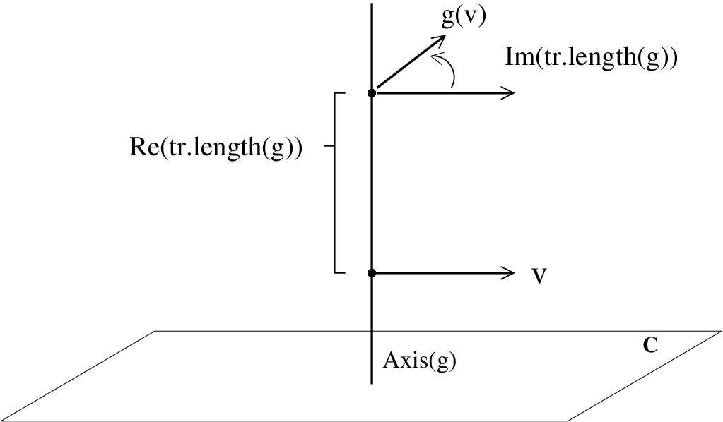
Let ${\mathbb{H}}^{n}$ denote $n$ -dimensional hyperbolic space, $Isom^{+}({\mathbb{H}}^{n})$ denote the group of orientation preserving isometries of ${\mathbb{H}}^{n}$ and $d(x,y)$ be the distance between points $x,y\in{\mathbb{H}}^{n}$ . If $g\in PSL_{2}({\mathbb{C}})=Isom^{+}({\mathbb{H}}^{3})$ is a hyperbolic (or loxodromic) isometry then its complex translation length $tr.length(g)\in{\mathbb{C}}$ is the complex number whose real part is the smallest number $r$ such that there is a $z\in{\mathbb{H}}^{3}$ such that $d(z,gz)=r$ and whose imaginary part measures the amount of rotation caused by $g$ . To be precise, if $Axis(g)$ denotes the axis of $g$ , $z\in Axis(g)$ and $v$ is a unit vector based at $z$ perpendicular to $Axis(g)$ then $Im(tr.length(g))$ is the angle from $\pi(v)$ to $gv$ where $\pi(v)$ equals $v$ parallel transported along $Axis(g)$ to lie in the tangent space of $g(z)$ . See figure 2.

Suppose $j_{*}:\pi_{1}(S)\to PSL_{2}({\mathbb{C}})$ is a representation. If $\gamma$ is a curve in $S$ then there is a unique conjugacy class $[\gamma]\subset\pi_{1}(S)$ representing it. Since conjugate elements of $PSL_{2}({\mathbb{C}})$ have the same translation length we can define the complex length of $\gamma$ (with respect to $j$ ) to be the complex translation length of any element in $j_{*}([\gamma])$ . We denote it by $length_{j}(\gamma)$ or $length(\gamma)$ when $j$ is understood.

Let $\gamma\in{\cal P}^{*}$ , $H_{1},H_{2}\in{\cal P}$ and $\gamma=\partial_{k}H_{1}=\partial_{k}H_{2}$ . Let $S^{\prime}=H\cup H^{\prime}$ . Assume that the representation $j_{*}$ restricts to a discrete faithful representation of $\pi_{1}(S^{\prime})$ and that the image contains no parabolics. If this is not the case, then we do not define $twist_{j}(\gamma)$ . Now let $\Gamma<PSL_{2}({\mathbb{C}})$ be the image $j_{*}(\pi_{1}(S^{\prime}))$ . By general homotopy theory there exists a map $j:S^{\prime}\to{\mathbb{H}}^{3}/\Gamma$ that induces the representation $j_{*}$ . Assume that $H_{1}$ is on the left of $\gamma$ and $H_{2}$ is on the right. After homotoping $j$ if necessary we may assume that $j$ maps each curve in ${\cal P}^{*}$ onto a geodesic. We may also assume that there exists an oriented path $m_{1}\subset S$ from $\partial_{k+1}H_{1}$ to $\gamma$ such that the length of $j(m_{1})$ is as small as possible (over all such paths in $S$ and over all maps $j^{\prime}$ homotopic to $j$ such that $j^{\prime}$ maps each curve in ${\cal P}^{*}$ to a geodesic). Similarly we may also assume that there exists an oriented path $m_{2}\subset S$ from $\gamma$ to $\partial_{k+1}H_{2}$ such that the length of $j(m_{2})$ is as small as possible (over all such paths in $S$ and over all maps $j^{\prime}$ homotopic to $j$ such that $j^{\prime}$ maps each curve in ${\cal P}^{*}$ to a geodesic).

It follows that $j(m_{1})$ and $j(m_{2})$ are geodesic segments perpendicular to the images of the respective boundary curves and the middle curve. Now we lift the image of the middle curve $j(\gamma)$ and $j(m_{1})$ and $j(m_{2})$ up to the universal cover ${\mathbb{H}}^{3}$ as shown in figure 3. We assume the lifting is done so that the union of the lifts is connected and the distance between the lift of $j(m_{1})$ and $j(m_{2})$ along the lift of $\gamma$ is as small as possible.

Let ${\tilde{m}_{i}}$ be the geodesic containing the lift of $j(m_{i})$ . Let $g\in PSL_{2}({\mathbb{C}})$ be the isometry whose axis is the lift of the image of $\gamma$ and such that $g({\tilde{m}}_{1})={\tilde{m}_{2}}$ (where ${\tilde{m}_{i}}$ is the oriented geodesic containing the lift of $j(m_{i})$ for $i=1,2$ ). Let $Axis(g)$ be oriented from its repelling point to its attracting point.

We define $twist_{j}(\gamma)=\pm tr.length(g)$ where the sign is positive if the orientation on $Axis(g)$ agrees with the orientation induced by $\gamma$ and is negative otherwise. This generalizes the previous definition of $twist(\gamma)$ (when $S$ was a totally geodesic surface). For example, if the imaginary part of $twist(\gamma)$ is small then the surface is only “lightly bent” at $\gamma$ .

Whether ${\cal M}$ is a product of surfaces or a $3$ -manifold the definition of $length_{j}(\cdot)$ and $twist_{j}(\cdot)$ depends only on the homotopy class of $j$ . Therefore, if $j_{*}:\pi_{1}(S)\to\pi_{1}({\cal M})$ is a homomorphism, then we may let $length_{j}(\cdot)$ and $twist_{j}(\cdot)$ be the length and twist parameter with respect to $j:S\to{\cal M}$ where $j$ is any map inducing $j_{*}$ .

7 The Horocyclic Flow

Let

N_{t}=\left[\begin{array}[]{cc}1&0\\ t&1\end{array}\right].

and let $N=\{N_{t}:t\in{\mathbb{R}}\}<PSL_{2}({\mathbb{R}})<PSL_{2}({\mathbb{C}})$ . Let ${\mathbb{F}}$ denote either ${\mathbb{R}}$ or ${\mathbb{C}}$ . If $\Gamma<PSL_{2}({\mathbb{F}})$ is discrete group, the horocyclic flow on the frame bundle $\Gamma\backslash PSL_{2}({\mathbb{F}})$ is the right action of $N$ on $\Gamma\backslash PSL_{2}({\mathbb{F}})$ .

Let $PSL^{2}_{2}({\mathbb{R}})$ denote $PSL_{2}({\mathbb{R}})\times PSL_{2}({\mathbb{R}})$ . If $\Gamma_{1},\Gamma_{2}<PSL_{2}({\mathbb{R}})$ are discrete groups, then the diagonal horocyclic flow on $(\Gamma_{1}\times\Gamma_{2})\backslash PSL^{2}_{2}({\mathbb{R}})$ is the action of the group ${\hat{N}}=\{(N_{t},N_{t})|t\in{\mathbb{R}}\}$ on $(\Gamma_{1}\times\Gamma_{2})\backslash PSL^{2}_{2}({\mathbb{R}})$ .

We say that $\Gamma_{1},\Gamma_{2}<PSL_{2}({\mathbb{R}})$ are commensurable if there exists an element $g\in PSL_{2}({\mathbb{R}})$ such that $g\Gamma_{1}g^{-1}\cap\Gamma_{2}$ has finite index in both $g\Gamma_{1}g^{-1}$ and $\Gamma_{2}$ . In such a case, if $S_{i}={\mathbb{H}}^{2}/\Gamma_{i}$ is a closed surface for $i=1,2$ then there exists a closed surface ${\tilde{S}}={\mathbb{H}}^{2}/\Gamma$ and local isometries $\pi_{i}:{\tilde{S}}\to S_{i}$ . In particular, the Ehrenpreis conjecture for $S_{1}$ and $S_{2}$ is trivial.

It seems likely that the following results are well-known. Except for the first statement below, we did not find them in the literature.

Theorem 7.1.

Let ${\mathbb{H}}_{2}/\Gamma_{1},{\mathbb{H}}_{2}/\Gamma_{2}$ be closed hyperbolic surfaces. Let $X=(\Gamma_{1}\times\Gamma_{2})\backslash(PSL_{2}({\mathbb{R}})\times PSL_{2}({\mathbb{R}}))$ . Then the following hold.

1.

Every orbit of the horocyclic flow in $\Gamma_{i}\backslash PSL_{2}({\mathbb{R}})$ is dense in $\Gamma_{i}\backslash PSL_{2}({\mathbb{R}})$ for $i=1,2$ .
2.

Every orbit of the diagonal horocyclic flow in $X$ is dense in $X$ unless $\Gamma_{1}$ and $\Gamma_{2}$ are commensurable.

Proof.

The first statement was proven by Hedlund [Hedlund1]. Let $\Gamma=\Gamma_{1}\times\Gamma_{2}$ . Let $g\in\Gamma$ . Then the closure of the ${\hat{N}}$ -orbit of $\Gamma g$ equals

\overline{\Gamma g{\hat{N}}}=\overline{\Gamma\backslash g{\hat{N}}g^{-1}}g\subset\Gamma\backslash PSL^{2}_{2}({\mathbb{R}}).

By Ratner’s theorems on unipotent flows [Ratner], there exists a closed subgroup $P$ of $PSL_{2}({\mathbb{R}})\times PSL_{2}({\mathbb{R}})$ such that $g{\hat{N}}g^{-1}<P$ and

\overline{\Gamma g{\hat{N}}g^{-1}}=\Gamma P.

Let $P_{0}$ be the component of $P$ containing the identity. By the classification of Lie subgroups of $PSL_{2}({\mathbb{R}})\times PSL_{2}({\mathbb{R}})$ and since $g{\hat{N}}g^{-1}$ is properly contained in $P_{0}$ , $P_{0}$ must be conjugate to one of the following.

1.

$B\times B$ (where $B<PSL_{2}({\mathbb{R}})$ is the set of upper triangular matrices).
2.

$\{(X,X)|\,X\in PSL_{2}({\mathbb{R}})\}$ .
3.

$PSL_{2}({\mathbb{R}})\times PSL_{2}({\mathbb{R}})$ .

By Hedlund’s result, for $k=1,2$ , $\overline{\Gamma g{\hat{N}}g^{-1}}$ projects onto $\Gamma_{k}\backslash PSL_{2}({\mathbb{R}})$ under the canonical projection map. Therefore the first possibility cannot occur. If the second possibility occurs then let $\pi:PSL_{2}({\mathbb{R}})\to{\mathbb{H}}^{2}=PSL_{2}({\mathbb{R}})/SO(2)$ by the quotient map. Then $(\pi\times\pi)(P)/\Gamma\subset({\mathbb{H}}^{2}\times{\mathbb{H}}^{2})/\Gamma$ is a closed hyperbolic surface and for $k=1,2$ , the projection maps from $({\mathbb{H}}^{2}\times{\mathbb{H}}^{2})/\Gamma$ to ${\mathbb{H}}^{2}/\Gamma_{k}$ are local isometries. This implies that $\Gamma_{1}$ and $\Gamma_{2}$ are commensurable.

The third possibility is equivalent to the statement that the ${\hat{N}}$ -orbit of $g$ in $\Gamma\backslash PSL^{2}_{2}({\mathbb{R}})$ is dense.

∎

The proof of the next theorem is similar to the previous theorem.

Theorem 7.2.

Let ${\cal M}={\mathbb{H}}^{3}/\Gamma$ be a closed hyperbolic $3$ -manifold where $\Gamma<PSL_{2}({\mathbb{C}})$ is a discrete cocompact group. Then either ${\cal M}$ contains a totally geodesic immersed closed surface or every orbit of the horocyclic flow in $\Gamma\backslash PSL_{2}({\mathbb{C}})$ is dense.

Part II The Isometry Construction

8 Sketch

Here we sketch the isometry construction in the 2-dimensional case. Suppose that $\Gamma<PSL_{2}({\mathbb{R}})$ is a discrete cocompact group. Let $a,b$ be distinct points in ${\mathbb{H}}^{2}$ . Let $v_{b}$ be the unit vector based at $b$ that points away from $a$ . Let $v_{a}$ be the unit vector based at $a$ that points towards $b$ . Then there is a unique isometry $\gamma\in PSL_{2}({\mathbb{R}})$ that maps $a$ to $b$ and $v_{a}$ to $v_{b}$ .

Suppose we would like $\gamma$ to be an element of $\Gamma$ but it is not. Then we perturb $\gamma$ so that it is an element of $\Gamma$ . To carry this out, let $\epsilon>0$ . Make the ray from $b$ through $a$ . It limits on a point $c$ on the circle at infinity. Let $h$ be the horocycle centered at $c$ that passes through $b$ . Now move the point $b$ along the horocycle $h$ and carry the vector $v_{b}$ along with it. Let $b(t)$ and $v_{b}(t)$ denote the point $b$ and the vector $v_{b}$ after time $t$ . As we move $v_{b}$ along the horocycle we look in its $\epsilon$ -neighborhood (with respect to some metric on the unit tangent bundle of ${\mathbb{H}}^{2}$ ). As soon as we see a $\Gamma$ translate of $v_{a}$ we stop. Let $v^{\prime}_{a}$ be the translate of $v_{a}$ that we first encounter. By definition then there is an isometry $g\in\Gamma$ such that $g(v_{a})=v^{\prime}_{a}$ . This isometry $g$ will be our new isometry, a perturbed copy of $\gamma$ . This is what we call the isometry construction (theorem 9.2). See figure 4.

Since every orbit of the horocycle flow on $\Gamma\backslash PSL_{2}({\mathbb{R}})$ is dense in $\Gamma\backslash PSL_{2}({\mathbb{R}})$ (theorem 7.1) the time $T$ at which we stop moving the point $b$ is bounded by a function of $\epsilon$ and $\Gamma$ . In particular, the bound does not depend on the points $a$ and $b$ .

Using this fact and some explicit calculations we will make estimates regarding the translation length of $g$ and the location of its axis. For instance, if the distance $d(a,b)=L$ between $a$ and $b$ is very large, then the translation length of $g$ will be about $\epsilon$ -close to $L$ . Just how large $L$ needs to be depends only on $\epsilon$ and $\Gamma$ . Other estimates will prove useful in bounding the geometry of not just a single isometry $g\in\Gamma$ but interesting subgroups of $\Gamma$ , mainly $2$ -generator free subgroups whose convex hull quotients are pairs of pants.

9 The Isometry Construction

Given $L>0$ , $T,\delta,\theta\in{\mathbb{R}}$ and $\nu\in{\mathbb{C}}$ let ${\it{\bf g}}={\it{\bf g}}(L,T,\nu,\delta,\theta)\in SL_{2}({\mathbb{C}})$ be defined by the following.

\begin{array}[]{l}{\it{\bf g}}=\left[\begin{array}[]{cc}\exp(L/2)&0\\ 0&\exp(-L/2)\end{array}\right]\left[\begin{array}[]{cc}1&0\\ T&1\end{array}\right]\left[\begin{array}[]{cc}e^{\nu}&0\\ 0&e^{-\nu}\end{array}\right]\left[\begin{array}[]{cc}\cos(\delta)&\sin(\delta)\\ -\sin(\delta)&\cos(\delta)\end{array}\right]\left[\begin{array}[]{cc}\exp(i\theta)&0\\ 0&\exp(-i\theta)\end{array}\right].\\ \end{array}

So,

{\it{\bf g}}=\left[\begin{array}[]{ccc}\exp(L/2+\nu+i\theta)\cos(\delta)&&\exp(L/2+\nu-i\theta)\sin(\delta)\\ \exp(-L/2)[Te^{\nu+i\theta}\cos(\delta)-e^{-\nu+i\theta}\sin(\delta)]&&\exp(-L/2)[Te^{\nu-i\theta}\sin(\delta)+e^{-\nu-i\theta}\cos(\delta)]\end{array}\right].

(5)

Proposition 9.1.

The translation length of $g={\it{\bf g}}(L,T,\nu,\delta,\theta)$ satisfies

tr.length(g)=L+2\nu+2i\theta+2\log(\cos(\delta))+O(\exp(-L)).

Moreover, the constant implicit in the $O(\cdot)$ notation depends only on an upper bound for $|T|$ and an upper bound for $|\nu|$ .

Proof.

From equation 5 we see that

	$\displaystyle trace(g)$	$\displaystyle=$	$\displaystyle\exp(L/2+\nu+i\theta)\cos(\delta)+\exp(-L/2+\nu-i\theta)T\sin(\delta)+\exp(-L/2-\nu-i\theta)\cos(\delta)$
		$\displaystyle=$	$\displaystyle\exp(L/2+\nu+i\theta)\cos(\delta)+O(\exp(-L/2)).$

Let $\mu$ be the displacement of $g$ when $Axis(g)$ is oriented from its repelling fixed point to its attracting fixed point. Then,

	$\displaystyle\cosh(\mu(g)/2)$	$\displaystyle=$	$\displaystyle trace(g)/2$
		$\displaystyle=$	$\displaystyle(1/2)\exp(L/2+\nu+i\theta)\cos(\delta)+O(\exp(-L/2)).$

This implies that

\displaystyle\mu(g)/2

\displaystyle=

\displaystyle L/2+\nu+i\theta+\log(\cos(\delta))+O(\exp(-L)).

Equivalently,

\displaystyle tr.length(g)

\displaystyle=

\displaystyle\mu(g)=L+2\nu+2i\theta+2\log(\cos(\delta))+O(\exp(-L)).

The last statement is easy to check.

∎

Theorem 9.2.

(The Isometry Construction, 2d and 3d case) Let ${\mathbb{F}}$ denote either ${\mathbb{R}}$ or ${\mathbb{C}}$ . Let $\Gamma<PSL_{2}({\mathbb{F}})$ be a cocompact discrete torsion-free orientation-preserving group. If ${\mathbb{F}}={\mathbb{C}}$ then assume that ${\mathbb{H}}^{3}/\Gamma$ does not contain an immersed totally geodesic closed surface. Let $\epsilon>0$ . Let $I_{r},I_{i}\subset[-\epsilon,\epsilon]$ be closed sets with nonempty interior.

Then there exists positive numbers ${\hat{T}}={\hat{T}}(\Gamma,\epsilon,I_{r},I_{i})$ and $L_{0}=L_{0}(\Gamma,\epsilon,I_{r},I_{i})$ such that for every orientation-preserving isometry $A\in PSL_{2}({\mathbb{F}})$ and for every $L>L_{0}$ there exists parameters $\delta,\theta\in{\mathbb{R}}$ and $T,\nu\in{\mathbb{C}}$ satisfying all of the following.

•

$g:=A^{-1}{\it{\bf g}}(L,T,\nu,\delta,\theta)A\in\Gamma$ .
•

$|\nu|,|\delta|,|\theta|,|\Im(T)|<\epsilon$ .
•

$|\Re(T)|<{\hat{T}}$ .
•

$tr.length(g)\in L+I_{r}+iI_{i}$ .
•

If ${\mathbb{F}}={\mathbb{R}}$ then $\Im(T)=\Im(\nu)=\theta=0$ .

In the above, we have abused notation by identifying ${\it{\bf g}}$ with its projection to $PSL_{2}({\mathbb{F}})$ .

Remark: To see how this is related to the sketch given in section 8, let $a$ be the point $(0,1)$ (in the upper half space model) and $b$ be the point $(0,\exp(L))$ . Then $g$ is the isometry ${\it{\bf g}}(L,T,\nu,\delta,0)$ .

Proof.

For any $\nu\in C$ and $\delta\in{\mathbb{R}}$ define matrices $C_{\nu},R_{\delta}\in SL_{2}({\mathbb{C}})$ by

\begin{array}[]{l}C_{\nu}=\left[\begin{array}[]{cc}e^{\nu}&0\\ 0&e^{-\nu}\end{array}\right]\\ \\ R_{\delta}=\left[\begin{array}[]{cc}\cos(\delta)&\sin(\delta)\\ -\sin(\delta)&\cos(\delta)\end{array}\right].\end{array}

Let $I^{\prime}_{r}$ be a closed subset contained in the interior of $I_{r}$ such that $I^{\prime}_{r}$ has nonempty interior. Let $I^{\prime}_{i}$ be a closed subset contained in the interior of $I_{i}$ such that $I^{\prime}_{i}$ has nonempty interior. Let $N_{t}\in SL_{2}({\mathbb{C}})$ be defined as in section 7. Let $B=B(\epsilon,I^{\prime}_{r},I^{\prime}_{i})\subset PSL_{2}({\mathbb{F}})$ be the set of all matrices of the form $N_{t}C_{\nu}R_{\delta}C_{i\theta}$ where

•

$\delta,\theta\in{\mathbb{R}}$
•

$t,\nu,i\theta\in{\mathbb{F}}$ ,
•

$|t|,|\delta|,|\nu|,|\theta|<\epsilon$ ,
•

$\Re(2\nu+2\log(\cos(\delta)))\in I^{\prime}_{r}$ and
•

$\Im(2\nu)+2\theta\in I^{\prime}_{i}$ .

Note $B$ has nonempty interior in $PSL_{2}({\mathbb{F}})$ . Theorem 7.1 and the hypothesis that either ${\mathbb{F}}={\mathbb{R}}$ or ${\mathbb{H}}^{3}/\Gamma$ does not contain an immersed totally geodesic closed surface imply that for every element $Z\in PSL_{2}({\mathbb{F}})$ the orbit

\{\Gamma ZN_{t}|\,t\in{\mathbb{R}}\}\subset\Gamma\backslash PSL_{2}({\mathbb{F}})

is dense in $\Gamma\backslash PSL_{2}({\mathbb{F}})$ . Since $\Gamma\backslash PSL_{2}({\mathbb{F}})$ is compact this implies that there exists a $T^{\prime}>0$ such that for all $Z_{1},Z_{2}\in PSL_{2}({\mathbb{F}})$ , there exists a $T$ with $|T|<T^{\prime}$ such that $\Gamma Z_{1}N_{T}\in\Gamma Z_{2}B^{-1}$ . We apply this fact to the isometries $Z_{1}=A^{-1}X$ and $Z_{2}=A^{-1}$ where $X=C_{L/2}$ .

So there exists a $T_{0}$ with $|T_{0}|<T^{\prime}$ and a $g\in\Gamma$ such that $A^{-1}XN_{T_{0}}=gA^{-1}(N_{t}C_{\nu}R_{\delta}C_{i\theta})^{-1}$ for some $\delta,\theta\in{\mathbb{R}}$ , $t,\nu\in{\mathbb{F}}$ with $N_{t}C_{\nu}R_{\delta}C_{i\theta}\in B$ . So,

g=A^{-1}XN_{T_{0}}N_{t}C_{\nu}R_{\delta}C_{i\theta}A=A^{-1}{\it{\bf g}}(L,T_{0}+t,\nu,\delta,\theta)A.

By proposition 9.1, $tr.length(g)=L+2\nu+2i\theta+2\cos(\delta)+O(\exp(-L))$ . Since $\Re(2\nu+2\cos(\delta))\in I^{\prime}_{r}\subset int(I_{r})$ and $\Im(2\nu)+2\theta\in I^{\prime}_{i}\subset int(I_{i})$ there exists an $L_{0}$ (that depends only on $T^{\prime}$ , $\epsilon$ and $\Gamma$ ) such that if $L>L_{0}$ then

tr.length(g)\in L+I_{r}+I_{i}.

To finish, let ${\hat{T}}=T^{\prime}+\epsilon$ . ∎

The proof of the theorem below is similar to the one above.

Theorem 9.3.

(The Isometry Construction, product of two surfaces case) Let $\Gamma_{1},\Gamma_{2}<PSL_{2}({\mathbb{R}})$ be two cocompact discrete torsion-free orientation-preserving groups. Assume that $\Gamma_{1}$ and $\Gamma_{2}$ are incommensurable. Let $\epsilon>0$ . Let $I_{1},I_{2}$ be two closed subsets of $[-\epsilon,\epsilon]$ such that both $I_{1}$ and $I_{2}$ have nonempty interior. Then there exists positive numbers ${\hat{T}}={\hat{T}}(\Gamma_{1},\Gamma_{2},\epsilon,I_{1},I_{2})$ , $L_{0}=L_{0}(\Gamma_{1},\Gamma_{2},\epsilon,I_{1},I_{2})>0$ such that the following holds.

For every pair of orientation-preserving isometries $(A_{1},A_{2})\in PSL_{2}({\mathbb{R}})\times PSL_{2}({\mathbb{R}})$ , for every $L>L_{0}$ and for $k=1,2$ there exists parameters $T_{k},\nu_{k},\delta_{k}\in{\mathbb{R}}$ such that all of the following statements hold.

•

$g_{k}:=A^{-1}_{k}{\it{\bf g}}(L,T_{k},\nu_{k},\delta_{k},0)A_{k}\in\Gamma_{k}$ .
•

$|T_{1}|,|T_{2}|<{\hat{T}}$ .
•

$|\delta_{k}|,|\nu_{k}|,|T_{1}-T_{2}|<\epsilon$ .
•

$tr.length(g_{k})\in L+I_{k}$ .

10 The Hexagon ${\cal H}$

Estimate Notation: Throughout this section when we write $x=O(f(L))$ the constants implicit in the $O(\cdot)$ notation will depend only on upper bounds for $|T|$ , $|\nu|$ and $|\delta|$ .

For this section we fix quantities $L,{\hat{T}},\delta,\theta,\alpha,\epsilon\in{\mathbb{R}}$ , $T,\nu,{\tilde{X}},{\tilde{M}}\in{\mathbb{C}}$ satisfying the bounds

•

$|T|<{\hat{T}}$ ,
•

$|\delta|,|\theta|,|\alpha|,|\nu|,|\Im(T)||<\epsilon$ ,
•

${\tilde{X}}=\exp(L/2)+O(\exp(L/4))$ and
•

${\tilde{M}}=e^{\alpha}M+O(\exp(-L/2))=2\exp(-L/4+\alpha)+O(\exp(-3L/2))$ where $M=M(L)$ is defined in corollary 5.2.

Let $g={\it{\bf g}}(L,T,\nu,\delta,\theta)$ . Let ${\cal H}={\cal H}(g,{\tilde{X}},{\tilde{M}})=({\tilde{H}}_{1},...,{\tilde{H}}_{6})$ be the standardly oriented right-angled hexagon satisfying the following (where ${H}_{k}=\mu({\tilde{H}}_{k-1},{\tilde{H}}_{k+1};{\tilde{H}}_{k})$ for all $k$ mod 6, see subsection 4.2).

1.

${\tilde{H}}_{1}$ is equal to the geodesic with endpoints $\{0,\infty\}$ (as unoriented geodesics).
2.

${\tilde{H}}_{3}$ is equal to the axis of $g$ (as unoriented geodesics).
3.

${\tilde{H}}_{6}$ has endpoints $\pm{\tilde{X}}$ .
4.

${H}_{6}={\tilde{M}}+i\pi$ .

Hexagon ${\cal H}$ is depicted in figure 5.

Theorem 10.1.

(Hexagon ${\cal H}$ estimates) Assume that $|\tan(\delta)|\leq 2\epsilon$ and $|e^{-2\nu}|\leq 2$ . Then:

$\displaystyle{H}_{2}$	$\displaystyle=$	$\displaystyle i\pi+O(\exp(-L/2)),$
$\displaystyle{H}_{4}$	$\displaystyle=$	$\displaystyle{\tilde{M}}+O(\exp(-L/2)),$
$\displaystyle{H}_{5}$	$\displaystyle=$	$\displaystyle(\sqrt{2}/2)\coth({\tilde{M}})\exp(-L/2)(T+\tau)+i\pi+O(\exp(-L/2))$

where $\tau\in{\mathbb{C}}$ is such that $|\tau|\leq 6\epsilon$ .

We now complete the proofs of the main theorems given the above result (which is proven in the next 4 subsections). Suppose ${\cal M}$ is a closed hyperbolic $3$ -manifold not containing any totally geodesic closed immersed surfaces. Let $\Gamma<PSL_{2}({\mathbb{C}})$ be a discrete group such that ${\cal M}$ is isometric to ${\mathbb{H}}^{3}/\Gamma$ . Suppose $S$ is a surface with a labeled pants decomposition ${\cal P}$ . Suppose $H\in{\cal P}$ is such that $\partial_{1}H\subset\partial S$ . Suppose $j_{*}:\pi_{1}(S)\to\Gamma$ is a discrete representation such that the restriction of $j_{*}$ to $\pi_{1}(H)<\pi_{1}(S)$ is faithful and without parabolics. Let $S^{\prime}\supset S$ be the (topological) surface extending $S$ such that $S^{\prime}$ has a labeled pants decomposition ${\cal P}^{\prime}$ extending ${\cal P}$ so that ${\cal P}^{\prime}-{\cal P}=\{H^{\prime}\}$ and $\partial_{1}H^{\prime}=\partial_{1}H$ . We will use the above theorem to extend $j_{*}$ to a homomorphism $j^{\prime}_{*}:\pi_{1}(S^{\prime})\to\Gamma$ satisfying certain geometric bounds.

Lemma 10.2.

Let $\epsilon>0$ be given. Then there exists an $L_{1}$ (depending only on $\Gamma$ and $\epsilon$ ) such that if $L>L_{1}$ and

\displaystyle\Big|length_{j}\big(\partial_{1}H\big)-L\Big|

\displaystyle\leq

\displaystyle\epsilon

then there exists a discrete representation $j^{\prime}_{*}:\pi_{1}(S^{\prime})\to\Gamma$ extending $j_{*}$ such that

$\displaystyle\Big\|length_{j^{\prime}}\big(\partial_{k}H^{\prime}\big)-L\Big\|$	$\displaystyle\leq$	$\displaystyle\epsilon\textnormal{ for $k=1,2,3$},$
$\displaystyle\Big\|\Re\big(twist_{j^{\prime}}(\partial_{1}H)\big)\Big\|$	$\displaystyle\leq$	$\displaystyle{\hat{T}}\exp(-L/4),$
$\displaystyle\Big\|\Im\big(twist_{j^{\prime}}(\partial_{1}H)\big)\Big\|$	$\displaystyle\leq$	$\displaystyle\epsilon\exp(-L/4)$

where ${\hat{T}}$ is a number depending only on ${\cal M}$ and $\epsilon$ .

Proof.

Let $I_{-}=[-\epsilon,-\epsilon/2]$ and $I_{+}=[\epsilon/2,\epsilon]$ . Choose $L_{1}$ to be larger than

\displaystyle\max\,L_{0}(\Gamma,\epsilon,I_{\sigma_{1}},I_{\sigma_{2}})

where $L_{0}(\cdot)$ is given by theorem 9.2 and the maximum is overall all $\sigma_{1},\sigma_{2}\in\{+,-\}$ . If necessary, choose $L_{1}$ larger so that for all $L>L_{1}$ the error estimates in theorem 10.1 and lemmas 5.1 and 5.3 are at most $\epsilon/8$ .

By general homotopy theory, there exists a map $j:S\to{\cal M}={\mathbb{H}}^{3}/\Gamma$ inducing $j_{*}$ . After homotoping $j$ we may assume that for $k=1,2,3$ , $j$ maps $\partial_{k}H$ to a geodesic. We may also assume that there exists a path $m$ from $\partial_{2}H$ to $\partial_{1}H$ such that the length of $j(m)$ is as small as possible over all such path and over all maps $j^{\prime}$ homotopic to $j$ that map the boundary of $H$ to geodesics. Thus $j(m)$ is a geodesic segment perpendicular to $j(\partial_{1}H)$ .

Let ${\tilde{m}}$ and $\gamma$ be lifts of $j(m)$ and $j(\partial_{1}H)$ respectively (so that ${\tilde{m}}\cup\gamma$ is a lift of $j(m)\cup j(\partial_{1}H)$ ). Orient ${\tilde{m}}$ towards $\gamma$ . Orient $\gamma$ to be consistent with the given orientation on $\partial_{1}H$ . Let $\eta$ be the oriented geodesic containing ${\tilde{m}}$ . Let $\Pi$ be the geodesic plane containing $\eta$ and $\gamma$ . Orient $\Pi$ so that $(v_{1},v_{2})$ forms a positively-oriented bases for $\Pi$ at $\gamma\cap\eta$ where $v_{1}$ points in the direction of $\eta$ and $v_{2}$ points in the direction of $\gamma$ . Let $p$ be a point on $\eta$ such that $d(p,\eta\cap\gamma)=M$ (where $M=M(L)$ is as in corollary 5.2) and $p$ comes after $\gamma\cap\eta$ with respect to the orientation on $\eta$ . See figure 6.

Let $A\in PSL_{2}({\mathbb{C}})$ be the orientation-preserving isometry that maps $\Pi$ to ${\mathbb{H}}^{2}$ (that is the plane bounded by the real line in the upperhalf-space model with the standard orientation), $\eta$ to the oriented geodesic from $-\exp(L/2)$ to $\exp(L/2)$ , and $p$ to $(0,\exp(L/2))$ .

Let $\rho_{1}\in{\mathbb{C}}$ be defined by $length(\partial H_{1})=L+\rho_{1}$ . Let $I_{r}=[\epsilon/2,\epsilon]$ or $[-\epsilon,-\epsilon/2]$ depending on whether $\Re(\rho_{1})$ is negative or positive. Similarly, let $I_{i}=[\epsilon/2,\epsilon]$ or $[-\epsilon,-\epsilon/2]$ depending on whether $\Im(\rho_{1})$ is negative or positive.

By the isometry construction theorem 9.2, there exists parameters $T,\nu,\delta,\theta$ such that

$\displaystyle\|T\|$	$\displaystyle\leq$	$\displaystyle{\hat{T}},$
$\displaystyle\|\nu\|,\|\delta\|,\|\theta\|,\|\Im(T)\|$	$\displaystyle\leq$	$\displaystyle\epsilon,$
$\displaystyle g_{3}:=A^{-1}{\it{\bf g}}(L,T,\nu,\delta,\theta)A$	$\displaystyle\in$	$\displaystyle\Gamma$
$\displaystyle tr.length(g_{3})$	$\displaystyle\in$	$\displaystyle L+I_{r}+iI_{i}.$

Let ${\cal H}=({\tilde{H}}_{1},...,{\tilde{H}}_{6})$ be the standardly oriented right-angled hexagon defined by

•

${\tilde{H}}_{5}$ is equal to $\gamma$ (as unoriented geodesics).
•

${\tilde{H}}_{3}$ is equal to the axis of $g_{3}$ (as unoriented geodesics).
•

${\tilde{H}}_{6}$ is equal to $\eta$ (as unoriented geodesics).
•

${\tilde{H}}_{1}\cap{\tilde{H}}_{6}=p$ so ${H}_{6}=M+i\pi$ where ${H}_{i}=\mu({\tilde{H}}_{i-1},{\tilde{H}}_{i+1};{\tilde{H}}_{i})$ for all $i$ mod $6$ .

Let ${\cal G}=({\tilde{G}}_{1},...,{\tilde{G}}_{6})$ and ${\cal F}=({\tilde{F}}_{1},...,{\tilde{F}}_{6})$ be the standardly oriented right-angled hexagons defined by

•

${\tilde{G}}_{1}={\tilde{F}}_{1}=\gamma$ but ${\tilde{G}}_{1}$ has the same orientation as $\gamma$ whereas ${\tilde{F}}_{1}$ has the opposite orientation,
•

${\tilde{G}}_{3}={\tilde{F}}_{2}=\eta$ (with orientation)
•

${\tilde{G}}_{3}={\tilde{F}}_{2}=Axis(g_{3})$ (as unoriented geodesics)
•

${G}_{1}={F}_{1}=length(\partial_{1}H)$ ,
•

${G}_{3}={F}_{3}=tr.length(g_{3})$ .

Here ${G}_{i}=\mu({\tilde{G}}_{i-1},{\tilde{G}}_{i+1};{\tilde{G}}_{i})$ and ${F}_{i}=\mu({\tilde{F}}_{i-1},{\tilde{F}}_{i+1};{\tilde{F}}_{i})$ for all $i$ mod $6$ . Let $\rho_{3},\rho_{5}\in{\mathbb{C}}$ be defined by $tr.length(g_{3})=L+\rho_{3}$ , ${G}_{5}=L/2+\rho_{5}/2+i\pi$ . The hypothesis and construction imply $|\rho_{1}|,|\rho_{3}|<\epsilon$ . By definition, ${G}_{2}={H}_{4}+i\pi$ . By the hexagon ${\cal H}$ estimates theorem above, this implies ${G}_{2}=M+O(\exp(-L/2))$ . Lemma 5.3 implies $\rho_{5}=\rho_{1}+\rho_{2}+O(\exp(-L/4))$ . By the hypotheses on $L_{1}$ , the error term is bounded by $\epsilon/8$ . This implies that $|\rho_{5}|<\epsilon$ .

Let $D_{G},D_{F}\subset{\mathbb{H}}^{3}$ be two disks with boundaries $\partial{\cal G}$ and $\partial{\cal F}$ . Here $\partial{\cal G}$ is the piecewise geodesic cycle with vertices $v_{i}={\tilde{G}}_{i}\cap{\tilde{G}}_{i+1}$ for $i$ mod $6$ (and similarly for $\partial{\cal F}$ ).

Let $g_{1}\in\Gamma$ be the hyperbolic element with axis $\gamma$ and translation length equal to $length(\partial_{1}H)$ . Clearly $(D_{G}\cup D_{F})/<g_{1},g_{3}>$ is a pair of pants $H^{\prime}$ where $<g_{1},g_{3}>$ denotes the group generated by $g_{1}$ and $g_{3}$ . We order the boundary components so that $\partial_{1}H^{\prime}$ is the image $\gamma$ , $\partial_{2}H^{\prime}$ is the image of $axis(g_{3})$ and $\partial_{3}H^{\prime}$ is the image of ${\tilde{G}}_{5}\cup{\tilde{F}}_{5}$ . The inclusion map $<g_{1},g_{3}><\Gamma$ induces a map $j^{\prime\prime}:H^{\prime}\to{\cal M}$ . $\partial_{1}H^{\prime}$ is identified with $\partial_{1}H$ as both are identified with $\gamma/g_{1}$ . So we may define $S^{\prime}=S\cup_{\partial_{1}H^{\prime}=\partial_{1}H}H^{\prime}$ and $j^{\prime}:S^{\prime}\to{\cal M}$ is the map extending both $j$ and $j^{\prime\prime}$ .

The length of $\partial_{3}H^{\prime}$ (with respect to $j^{\prime}$ ) is $2{G}_{5}=L+\rho_{5}$ . The twist parameter at $\partial_{1}H$ is, by definition, equal to ${H}_{5}-i\pi$ . By the previous theorem this real part bounded by $10{\hat{T}}\exp(-L/4)$ and imaginary part bounded by $100\epsilon\exp(-L/4)$ . Since $\epsilon$ is arbitrary this concludes the lemma. ∎

Proof.

(of theorem 1.10)

Let ${\cal M}$ be a closed hyperbolic 3-manifold. Suppose that there does not exist any closed totally geodesic surface immersed in ${\cal M}$ . We identify ${\cal M}$ with ${\mathbb{H}}^{3}/\Gamma$ for some cocompact discrete group $\Gamma<PSL_{2}({\mathbb{C}})$ . Let $\epsilon>0$ . Let $L_{0}=L_{1}$ be given by the previous lemma. Let $L>L_{0}$ .

Using the proof of the above lemma, it can be shown that there exists a map $j:H\to{\cal M}$ from a boundary-ordered pair of pants into ${\cal M}$ such that

\displaystyle\Big|length_{j}\big(\partial_{k}H\big)-L\Big|

\displaystyle\leq

\displaystyle\epsilon

for $k=1,2,3$ . Applying the lemma successively, we obtain a map $j^{\prime}:S\to{\cal M}$ from a surface $S$ into $M$ satisfying the conclusions of the theorem.

∎

The proof of theorem 1.3 involves only notational changes to the above proof so we omit it.

10.1 Fixed Points of ${\it{\bf g}}$

Let $\{e_{0},e_{1}\}\subset{\mathbb{C}}$ be the fixed points of ${\it{\bf g}}$ . Let

\begin{array}[]{ll}N_{1}&=\exp(L/2+\nu+i\theta)\cos(\delta)-\exp(-L/2+\nu-i\theta)T\sin(\delta)-\exp(-L/2-\nu-i\theta)\cos(\delta).\\ N_{2}&=\Big[\Big(\exp(L/2+\nu+i\theta)\cos(\delta)+\exp(-L/2-i\theta)\big(e^{\nu}T\sin(\delta)+e^{-\nu}\cos(\delta)\big)\Big)^{2}-4\Big]^{1/2}.\\ D&=2\exp(-L/2)[Te^{\nu+i\theta}\cos(\delta)-e^{-\nu+i\theta}\sin(\delta)].\end{array}

From equation 2 (subsection 3.2) and equation 5 (section 9) we obtain

\{e_{0},e_{1}\}=\left\{\frac{N_{1}-N_{2}}{D},\frac{N_{1}+N_{2}}{D}\right\}.

(6)

After relabeling if necessary we may assume $e_{0}=(N_{1}-N_{2})/D$ and $e_{1}=(N_{1}+N_{2})/D$ . When $L$ is large and the other parameters are small, $e_{0}$ is close to zero and $e_{1}$ is “close” to $\infty$ . The next proposition will be useful in estimating the widths of the hexagon ${\cal H}$ and the pentagon ${\cal K}$ .

Proposition 10.3.

The following estimates and identities hold:

$\displaystyle N_{1}$	$\displaystyle\approx$	$\displaystyle\exp(L/2).$
$\displaystyle N_{2}$	$\displaystyle\approx$	$\displaystyle\exp(L/2).$
$\displaystyle N_{1}-N_{2}$	$\displaystyle=$	$\displaystyle O(\exp(-L/2)).$
$\displaystyle N_{1}+N_{2}$	$\displaystyle\approx$	$\displaystyle\exp(L/2).$
$\displaystyle N_{1}^{2}-N_{2}^{2}$	$\displaystyle=$	$\displaystyle O(1).$
$\displaystyle D$	$\displaystyle=$	$\displaystyle O(\exp(-L/2)).$
$\displaystyle\frac{N_{1}^{2}-N_{2}^{2}}{D}$	$\displaystyle=$	$\displaystyle-2\sin(\delta)\exp(L/2+\nu-i\theta)=O(\exp(L/2)).$
$\displaystyle\frac{\frac{N_{1}^{2}-N_{2}^{2}}{D}+D\exp(L)}{\exp(L/2)N_{2}}$	$\displaystyle=$	$\displaystyle O(\exp(-L/2)).$

Proof.

The estimates for $N_{1},N_{2},N_{1}+N_{2}$ and $D$ are immediate. Recall that for $x$ close to zero, $\sqrt{1-x}=1-(1/2)x+O(x^{2})$ . So if $x$ is very large, $\sqrt{x^{2}-4}=x\sqrt{1-4/x^{2}}=x-2/x+O(1/x^{3})$ . Hence,

\displaystyle N_{2}

\displaystyle=

\displaystyle\exp(L/2+\nu+i\theta)\cos(\delta)+O(\exp(-L/2)).

Thus $N_{1}-N_{2}=O(\exp(-L/2))$ as required. We compute $N_{1}^{2}-N_{2}^{2}$ as follows:

$\displaystyle N_{1}^{2}-N_{2}^{2}$	$\displaystyle=$	$\displaystyle\Big(\exp(L/2+\nu+i\theta)\cos(\delta)-\exp(-L/2-i\theta)\big(e^{\nu}T\sin(\delta)+e^{-\nu}\cos(\delta)\big)\Big)^{2}$
		$\displaystyle-\Big(\exp(L/2+\nu+i\theta)\cos(\delta)+\exp(-L/2-i\theta)\big(e^{\nu}T\sin(\delta)+e^{-\nu}\cos(\delta)\big)\Big)^{2}+4$
	$\displaystyle=$	$\displaystyle-4\exp(\nu)\cos(\delta)\Big(\exp(\nu)T\sin(\delta)+\exp(-\nu)\cos(\delta)\Big)+4$
	$\displaystyle=$	$\displaystyle 4\sin(\delta)e^{\nu}\Big(e^{-\nu}\sin(\delta)-e^{\nu}T\cos(\delta)\Big)=O(1).$

Therefore,

	$\displaystyle\frac{N_{1}^{2}-N_{2}^{2}}{D}$	$\displaystyle=$	$\displaystyle\frac{4\sin(\delta)e^{\nu}[e^{-\nu}\sin(\delta)-e^{\nu}T\cos(\delta)]}{2\exp(-L/2+i\theta)[Te^{\nu}\cos(\delta)-e^{-\nu}\sin(\delta)]}$
		$\displaystyle=$	$\displaystyle-2\sin(\delta)\exp(L/2+\nu-i\theta)=O(\exp(L/2)).$

Since $D\exp(L)=O(\exp(L/2))$ and $\exp(L/2)N_{2}\approx\exp(L)$ this implies that

\displaystyle\frac{\frac{N_{1}^{2}-N_{2}^{2}}{D}+D\exp(L)}{\exp(L/2)N_{2}}=O(\exp(-L/2))

as required. ∎

10.2 The Width ${H}_{2}$

In this subsection we prove:

Proposition 10.4.

The width ${H}_{2}$ satisfies

\begin{array}[]{ll}\cosh({H}_{2})&=-N_{1}/N_{2}.\\ {H}_{2}&=i\pi+O(\exp(-L/2)).\end{array}

Proof.

Recall the definition of the cross ratio $R$ (subsection 4.1). Let

R:=R(\infty,0,e_{0},e_{1})=\frac{e_{1}}{e_{0}}=\frac{N_{1}+N_{2}}{N_{1}-N_{2}}.

Recall that ${H}_{2}=\mu({\tilde{H}}_{1},{\tilde{H}}_{3};{\tilde{H}}_{2})$ . By subsection 4.2, $\tanh^{2}(\mu({\tilde{H}}_{1},{\tilde{H}}_{3};{\tilde{H}}_{2})/2)=R$ . So

\displaystyle\cosh({H}_{2})=\frac{1+R}{1-R}=\frac{-N_{1}}{N_{2}}.

This proves the first statement. Note

N_{1}/N_{2}=1+\frac{N_{1}-N_{2}}{N_{2}}=1+O(\exp(-L))

since $N_{1}-N_{2}=O(\exp(-L/2))$ and $N_{2}\approx\exp(L/2)$ by the previous proposition. So ${H}_{2}=i\pi+O(\exp(-L/2))$ as required.

∎

10.3 The Width ${H}_{4}$

Proposition 10.5.

Let $\{f_{0},f_{1}\}$ be the endpoints of ${\tilde{H}}_{5}$ with $|f_{0}|<|f_{1}|$ . Let ${\bar{M}}=\tanh({\tilde{M}}/2)$ . Then

\begin{array}[]{ll}f_{0}&=-{\bar{M}}{\tilde{X}}\\ f_{1}&=-{\tilde{X}}/{\bar{M}}.\end{array}

Proof.

By definition ${\tilde{H}}_{5}$ is orthogonal to the geodesic with endpoints $\{-{\tilde{X}},{\tilde{X}}\}$ . Thus

R(f_{0},f_{1},{\tilde{X}},-{\tilde{X}})=\tanh^{2}(i\pi/4)=-1.

So,

\frac{(f_{0}-{\tilde{X}})(f_{1}+{\tilde{X}})}{(f_{0}+{\tilde{X}})(f_{1}-{\tilde{X}})}=-1.

Equivalently,

f_{0}f_{1}+(f_{0}-f_{1}){\tilde{X}}-{\tilde{X}}^{2}=-f_{0}f_{1}+(f_{0}-f_{1}){\tilde{X}}+{\tilde{X}}^{2}.

So, $f_{0}f_{1}={\tilde{X}}^{2}$ . The width ${H}_{6}=\mu({\tilde{H}}_{5},{\tilde{H}}_{1};{\tilde{H}}_{6})$ equals ${\tilde{M}}$ . By subsection 4.2 $R(f_{0},f_{1},0,\infty)=\tanh^{2}({H}_{6}/2)$ . So,

\frac{(f_{0}-0)(f_{1}-\infty)}{(f_{0}-\infty)(f_{1}-0)}=\frac{f_{0}}{f_{1}}=\tanh^{2}({\tilde{M}}/2).

Thus

	$\displaystyle f_{0}^{2}$	$\displaystyle=$	$\displaystyle f_{0}f_{1}\frac{f_{0}}{f_{1}}=\tanh^{2}({\tilde{M}}/2){\tilde{X}}^{2}=(-{\bar{M}}{\tilde{X}})^{2}\textrm{ and}$
	$\displaystyle f_{1}^{2}$	$\displaystyle=$	$\displaystyle f_{0}f_{1}\frac{f_{1}}{f_{0}}=\coth^{2}({\tilde{M}}/2){\tilde{X}}^{2}=(-{\tilde{X}}/{\bar{M}})^{2}.$

The choice of sign is justified by figure 5.

∎

Proposition 10.6.

The width ${H}_{4}$ satisfies:

$\displaystyle\cosh({H}_{4})$	$\displaystyle=$	$\displaystyle(N_{1}/N_{2})\cosh({\tilde{M}})+(1/2)\sinh({\tilde{M}})Z;$
$\displaystyle\sinh({H}_{4})$	$\displaystyle=$	$\displaystyle\sinh({\tilde{M}})+(1/2)\cosh({\tilde{M}})Z-(1/4)\cosh({\tilde{M}})\coth({\tilde{M}})Q+O(\exp(-L));$
$\displaystyle{H}_{4}$	$\displaystyle=$	$\displaystyle{\tilde{M}}+O(\exp(-L/2)).$

where

	$\displaystyle Z$	$\displaystyle=$	$\displaystyle\frac{D{\tilde{X}}^{2}+(N_{1}^{2}-N_{2}^{2})/D}{{\tilde{X}}N_{2}}=O(\exp(-L/2)),$
	$\displaystyle Q$	$\displaystyle=$	$\displaystyle\frac{D^{2}{\tilde{X}}^{4}+(N_{1}^{2}-N_{2}^{2})^{2}/D^{2}}{{\tilde{X}}^{2}N_{2}^{2}}=O(\exp(-L)).$

Proof.

We compute $R(f_{0},f_{1},e_{0},e_{1})$ as follows.

$\displaystyle R(f_{0},f_{1},e_{0},e_{1})$	$\displaystyle=$	$\displaystyle\frac{(-{\bar{M}}{\tilde{X}}-\frac{N_{1}-N_{2}}{D})(-{\tilde{X}}/{\bar{M}}-\frac{N_{1}+N_{2}}{D})}{(-{\bar{M}}{\tilde{X}}-\frac{N_{1}+N_{2}}{D})(-{\tilde{X}}/{\bar{M}}-\frac{N_{1}-N_{2}}{D})}$
	$\displaystyle=$	$\displaystyle\frac{(-D{\bar{M}}{\tilde{X}}-(N_{1}-N_{2}))(-D{\tilde{X}}-{\bar{M}}(N_{1}+N_{2}))}{(-D{\bar{M}}{\tilde{X}}-(N_{1}+N_{2}))(-D{\tilde{X}}-{\bar{M}}(N_{1}-N_{2}))}$
	$\displaystyle=$	$\displaystyle\frac{D^{2}{\bar{M}}{\tilde{X}}^{2}+D{\tilde{X}}(N_{1}-N_{2})+D{\bar{M}}^{2}{\tilde{X}}(N_{1}+N_{2})+{\bar{M}}(N_{1}^{2}-N_{2}^{2})}{D^{2}{\bar{M}}{\tilde{X}}^{2}+D{\tilde{X}}(N_{1}+N_{2})+D{\bar{M}}^{2}{\tilde{X}}(N_{1}-N_{2})+{\bar{M}}(N_{1}^{2}-N_{2}^{2})}$
	$\displaystyle=$	$\displaystyle\frac{D{\bar{M}}{\tilde{X}}^{2}+{\tilde{X}}(N_{1}-N_{2})+{\bar{M}}^{2}{\tilde{X}}(N_{1}+N_{2})+{\bar{M}}(N_{1}^{2}-N_{2}^{2})/D}{D{\bar{M}}{\tilde{X}}^{2}+{\tilde{X}}(N_{1}+N_{2})+{\bar{M}}^{2}{\tilde{X}}(N_{1}-N_{2})+{\bar{M}}(N_{1}^{2}-N_{2}^{2})/D}=(a/b)$

where $a$ is the numerator in the line above and $b$ is the denominator. Since $R=\tanh^{2}({H}_{4}/2)$ we obtain the following.

$\displaystyle\cosh({H}_{4})$	$\displaystyle=$	$\displaystyle\frac{1+R}{1-R}=\frac{1+(a/b)}{1-(a/b)}=\frac{b+a}{b-a}$
	$\displaystyle=$	$\displaystyle\frac{2D{\bar{M}}{\tilde{X}}^{2}+2(1+{\bar{M}}^{2}){\tilde{X}}N_{1}+2{\bar{M}}(N_{1}^{2}-N_{2}^{2})/D}{2(1-{\bar{M}}^{2}){\tilde{X}}N_{2}}$
	$\displaystyle=$	$\displaystyle\frac{(1+{\bar{M}}^{2}){\tilde{X}}N_{1}}{(1-{\bar{M}}^{2}){\tilde{X}}N_{2}}+\frac{D{\bar{M}}{\tilde{X}}^{2}+{\bar{M}}(N_{1}^{2}-N_{2}^{2})/D}{(1-{\bar{M}}^{2}){\tilde{X}}N_{2}}$
	$\displaystyle=$	$\displaystyle\cosh({\tilde{M}})(N_{1}/N_{2})+\frac{{\bar{M}}}{1-{\bar{M}}^{2}}\left(\frac{D{\tilde{X}}^{2}+(N_{1}^{2}-N_{2}^{2})/D}{{\tilde{X}}N_{2}}\right)$
	$\displaystyle=$	$\displaystyle\cosh({\tilde{M}})(N_{1}/N_{2})+(1/2)\sinh({\tilde{M}})\left(\frac{D{\tilde{X}}^{2}+(N_{1}^{2}-N_{2}^{2})/D}{{\tilde{X}}N_{2}}\right)$
	$\displaystyle=$	$\displaystyle\cosh({\tilde{M}})(N_{1}/N_{2})+(1/2)\sinh({\tilde{M}})Z.$

This proves the first statement. Let $X=\exp(L/2)$ . Then

$\displaystyle Z$	$\displaystyle=$	$\displaystyle\frac{D{\tilde{X}}^{2}+(N_{1}^{2}-N_{2}^{2})/D}{{\tilde{X}}N_{2}}$
	$\displaystyle=$	$\displaystyle\frac{D(X^{2}+O(\exp(3L/4)))+(N_{1}^{2}-N_{2}^{2})/D}{(X+O(\exp(L/4)))N_{2}}$
	$\displaystyle=$	$\displaystyle\frac{DX^{2}+(N_{1}^{2}-N_{2}^{2})/D}{XN_{2}}+O(\exp(-3L/4))$
	$\displaystyle=$	$\displaystyle O(\exp(-L/2)).$

The last estimate comes from proposition 10.3. Now we estimate $\sinh({H}_{4})$ .

			$\displaystyle\sinh({H}_{4})=\left(\cosh^{2}({H}_{4})-1\right)^{1/2}$
		$\displaystyle=$	$\displaystyle\left(\left(\cosh({\tilde{M}})(N_{1}/N_{2})+(1/2)\sinh({\tilde{M}})Z\right)^{2}-1\right)^{1/2}$
		$\displaystyle=$	$\displaystyle\left(\cosh^{2}({\tilde{M}})(N_{1}/N_{2})^{2}+\cosh({\tilde{M}})\sinh({\tilde{M}})Z(N_{1}/N_{2})+(1/4)\sinh^{2}({\tilde{M}})Z^{2}-1\right)^{1/2}$
		$\displaystyle=$	$\displaystyle\left(\sinh^{2}({\tilde{M}})+\cosh^{2}({\tilde{M}})[(N_{1}/N_{2})^{2}-1]+\cosh({\tilde{M}})\sinh({\tilde{M}})Z(N_{1}/N_{2})+(1/4)\sinh^{2}({\tilde{M}})Z^{2}\right)^{1/2}$
		$\displaystyle=$	$\displaystyle\sinh({\tilde{M}})\left(1+\coth^{2}({\tilde{M}})[(N_{1}/N_{2})^{2}-1]+\coth({\tilde{M}})Z(N_{1}/N_{2})+(1/4)Z^{2}\right)^{1/2}$
		$\displaystyle=$	$\displaystyle\sinh({\tilde{M}})\left(1+\coth^{2}({\tilde{M}})[(N_{1}/N_{2})^{2}-1]+\coth({\tilde{M}})Z+O(\exp(-L))\right)^{1/2}.$

We check the order of magnitude of the terms above. Since $N_{1}^{2}-N_{2}^{2}=O(1)$ and $N_{2}^{2}\approx\exp(-L)$ the term $[(N_{1}/N_{2})^{2}-1]=[N_{1}^{2}-N_{2}^{2}]/N_{2}^{2}=O(\exp(-L))$ . Since ${\tilde{M}}\approx\exp(-L/4)$ , $\coth({\tilde{M}})\approx\exp(L/4)$ . So

\coth^{2}({\tilde{M}})[(N_{1}/N_{2})^{2}-1]=O(\exp(-L/2)).

Since $Z=O(\exp(-L/2))$ we have that $\coth({\tilde{M}})Z=O(\exp(-L/4))$ . So the expression above is equal to $\sinh({\tilde{M}})\sqrt{1+x}$ where $x=O(\exp(-L/4))$ . Recall that $\sqrt{1+x}=1+(1/2)x-(1/4)x^{2}+O(x^{3})$ . So

			$\displaystyle\sinh({H}_{4})$
		$\displaystyle=$	$\displaystyle\sinh({\tilde{M}})\big(1+(1/2)\coth^{2}({\tilde{M}})[(N_{1}/N_{2})^{2}-1]+(1/2)\coth({\tilde{M}})Z+O(\exp(-L))$
			$\displaystyle-(1/4)\big[\coth^{2}({\tilde{M}})[(N_{1}/N_{2})^{2}-1]+\coth({\tilde{M}})Z+O(\exp(-L))\big]^{2}+O(\exp(-3L/4))\big)$
		$\displaystyle=$	$\displaystyle\sinh({\tilde{M}})\big(1+(1/2)\coth^{2}({\tilde{M}})[(N_{1}/N_{2})^{2}-1]+(1/2)\coth({\tilde{M}})Z+O(\exp(-L))$
			$\displaystyle-(1/4)[\coth({\tilde{M}})Z+O(\exp(-L/2))]^{2}+O(\exp(-3L/4))\big)$
		$\displaystyle=$	$\displaystyle\sinh({\tilde{M}})+(1/2)\cosh({\tilde{M}})Z+(1/2)\cosh({\tilde{M}})\coth({\tilde{M}})[(N_{1}/N_{2})^{2}-1]$
			$\displaystyle-(1/4)\cosh({\tilde{M}})\coth({\tilde{M}})Z^{2}+O(\exp(-L))$
		$\displaystyle=$	$\displaystyle\sinh({\tilde{M}})+(1/2)\cosh({\tilde{M}})Z$
			$\displaystyle+(1/2)\cosh({\tilde{M}})\coth({\tilde{M}})\left([(N_{1}/N_{2})^{2}-1]-(1/2)Z^{2}\right)+O(\exp(-L)).$

We estimate the last coefficient:

$\displaystyle[(N_{1}/N_{2})^{2}-1]-(1/2)Z^{2}$	$\displaystyle=$	$\displaystyle\frac{N_{1}^{2}-N_{2}^{2}}{N_{2}^{2}}-(1/2)\left(\frac{D{\tilde{X}}^{2}+(N_{1}^{2}-N_{2}^{2})/D}{{\tilde{X}}N_{2}}\right)^{2}$
	$\displaystyle=$	$\displaystyle\frac{N_{1}^{2}-N_{2}^{2}}{N_{2}^{2}}-(1/2)\frac{D^{2}{\tilde{X}}^{4}+(N_{1}^{2}-N_{2}^{2})^{2}/D^{2}+2{\tilde{X}}^{2}(N_{1}^{2}-N_{2}^{2})}{{\tilde{X}}^{2}N_{2}^{2}}$
	$\displaystyle=$	$\displaystyle-(1/2)\frac{D^{2}{\tilde{X}}^{4}+(N_{1}^{2}-N_{2}^{2})^{2}/D^{2}}{{\tilde{X}}^{2}N_{2}^{2}}=-(1/2)Q.$

$D^{2}{\tilde{X}}^{4}=O(\exp(L))$ since $D=O(\exp(-L/2))$ and ${\tilde{X}}\approx\exp(L/2)$ . The previous proposition implies $(N_{1}^{2}-N_{2}^{2})^{2}/D^{2}=O(\exp(L))$ . So the numerator is on the order of $\exp(L)$ . Since $N_{2}\approx\exp(L)$ the denominator ${\tilde{X}}^{2}N_{2}^{2}\approx\exp(2L)$ . Thus $Q=O(\exp(-L))$ . Thus we have:

\sinh({H}_{4})=\sinh({\tilde{M}})+(1/2)\cosh({\tilde{M}})Z-(1/4)\cosh({\tilde{M}})\coth({\tilde{M}})Q+O(\exp(-L))

as required. Next we compute $\sinh({H}_{4}-{\tilde{M}})$ as follows.

$\displaystyle\sinh({H}_{4}-{\tilde{M}})$	$\displaystyle=$	$\displaystyle\sinh({H}_{4})\cosh({\tilde{M}})-\cosh({H}_{4})\sinh({\tilde{M}})$
	$\displaystyle=$	$\displaystyle\cosh({\tilde{M}})\sinh({\tilde{M}})+(1/2)\cosh^{2}({\tilde{M}})Z-(1/4)\cosh^{2}({\tilde{M}})\coth({\tilde{M}})Q$
		$\displaystyle+O(\exp(-L))-\cosh({\tilde{M}})\sinh({\tilde{M}})-(1/2)\sinh^{2}({\tilde{M}})Z+O(\exp(-5L/4))$
	$\displaystyle=$	$\displaystyle(1/2)Z-(1/4)\cosh^{2}({\tilde{M}})\coth({\tilde{M}})Q+O(\exp(-L))$
	$\displaystyle=$	$\displaystyle O(\exp(-L/2)).$

∎

10.4 The Width ${H}_{5}$

Proposition 10.7.

Assume that $|\tan(\delta)|\leq 2\epsilon$ and $|e^{-2\nu}|\leq 2$ . Then we have the following estimates:

{H}_{5}=(\sqrt{2}/2)\coth({\tilde{M}})\exp(-L/2)(T+\tau)+i\pi+O(\exp(-L/2))

where $\tau\in{\mathbb{C}}$ is such that $|\tau|\leq 6\epsilon$ .

Proof.

Recall that ${H}_{6}={\tilde{M}}+i\pi$ . By the law of cosines we obtain

$\displaystyle\cosh({H}_{5})$	$\displaystyle=$	$\displaystyle\frac{\cosh({H}_{2})-\cosh({H}_{6})\cosh({H}_{4})}{\sinh({H}_{6})\sinh({H}_{4})}$
	$\displaystyle=$	$\displaystyle\frac{-N_{1}/N_{2}+\cosh({\tilde{M}})[(N_{1}/N_{2})\cosh({\tilde{M}})+(1/2)\sinh({\tilde{M}})Z]}{-\sinh({\tilde{M}})[\sinh({\tilde{M}})+(1/2)\cosh({\tilde{M}})Z-(1/4)\cosh({\tilde{M}})\coth({\tilde{M}})Q+O(\exp(-L))]}$
	$\displaystyle=$	$\displaystyle\frac{(N_{1}/N_{2})\sinh^{2}({\tilde{M}})+(1/2)\cosh({\tilde{M}})\sinh({\tilde{M}})Z}{-\sinh({\tilde{M}})[\sinh({\tilde{M}})+(1/2)\cosh({\tilde{M}})Z-(1/4)\cosh({\tilde{M}})\coth({\tilde{M}})Q+O(\exp(-L))]}$
	$\displaystyle=$	$\displaystyle-\frac{\sinh({\tilde{M}})(N_{1}/N_{2})+(1/2)\cosh({\tilde{M}})Z}{\sinh({\tilde{M}})+(1/2)\cosh({\tilde{M}})Z-(1/4)\cosh({\tilde{M}})\coth({\tilde{M}})Q}+O(\exp(-3L/4))$
	$\displaystyle=$	$\displaystyle-1-\frac{\sinh({\tilde{M}})(N_{1}/N_{2}-1)+(1/4)\cosh({\tilde{M}})\coth({\tilde{M}})Q}{\sinh({\tilde{M}})+(1/2)\cosh({\tilde{M}})Z-(1/4)\cosh({\tilde{M}})\coth({\tilde{M}})Q}+O(\exp(-3L/4))$
	$\displaystyle=$	$\displaystyle-1-\frac{(1/4)\cosh({\tilde{M}})\coth({\tilde{M}})Q}{\sinh({\tilde{M}})}+O(\exp(-3L/4))$
	$\displaystyle=$	$\displaystyle-1-(1/4)\coth^{2}({\tilde{M}})Q+O(\exp(-3L/4)).$

The issue now is to compute $\sqrt{Q}$ . Recall that

$\displaystyle Q$	$\displaystyle=$	$\displaystyle\frac{D^{2}{\tilde{X}}^{4}+(N_{1}^{2}-N_{2}^{2})^{2}/D^{2}}{{\tilde{X}}^{2}N_{2}^{2}}$
$\displaystyle(N_{1}^{2}-N_{2}^{2})^{2}/D^{2}$	$\displaystyle=$	$\displaystyle[-2\sin(\delta)\exp(L/2+\nu-i\theta)]^{2}$
$\displaystyle D$	$\displaystyle=$	$\displaystyle 2\exp(-L/2+i\theta)[Te^{\nu}\cos(\delta)-e^{-\nu}\sin(\delta)]$
$\displaystyle N_{2}^{2}$	$\displaystyle=$	$\displaystyle\Big(\exp(L/2+\nu+i\theta)\cos(\delta)+\exp(-L/2-i\theta)\big(e^{\nu}T\sin(\delta)+e^{-\nu}\cos(\delta)\big)\Big)^{2}-4.$

Next we estimate $Q$ . Let $X=\exp(L/2)$ .

$\displaystyle Q$	$\displaystyle=$	$\displaystyle\frac{D^{2}{\tilde{X}}^{4}+(N_{1}^{2}-N_{2}^{2})^{2}/D^{2}}{{\tilde{X}}^{2}N_{2}^{2}}$
	$\displaystyle=$	$\displaystyle\frac{D^{2}(X+O(\exp(L/4)))^{4}+(N_{1}^{2}-N_{2}^{2})^{2}/D^{2}}{(X+O(\exp(L/4)))^{2}N_{2}^{2}}$
	$\displaystyle=$	$\displaystyle\frac{D^{2}X^{4}+(N_{1}^{2}-N_{2}^{2})^{2}/D^{2}}{X^{2}N_{2}^{2}}+O(\exp(-5L/4)).$

So,

$\displaystyle Q$	$\displaystyle=$	$\displaystyle X^{-2}\frac{4\exp(L+2i\theta)[Te^{\nu}\cos(\delta)-e^{-\nu}\sin(\delta)]^{2}+[-2\sin(\delta)\exp(L/2+\nu-i\theta)]^{2}}{\big[\exp(L/2+\nu+i\theta)\cos(\delta)+\exp(-L/2-i\theta)\big(e^{\nu}T\sin(\delta)+e^{-\nu}\cos(\delta)\big)\big]^{2}-4}$
		$\displaystyle+O(\exp(-5L/4))$
	$\displaystyle=$	$\displaystyle\frac{4e^{2i\theta}[Te^{\nu}\cos(\delta)-e^{-\nu}\sin(\delta)]^{2}+4\sin^{2}(\delta)e^{2\nu-2i\theta}}{\big[\exp(L/2+\nu+i\theta)\cos(\delta)+\exp(-L/2-i\theta)\big(e^{\nu}T\sin(\delta)+e^{-\nu}\cos(\delta)\big)\big]^{2}-4}+O(\exp(-5L/4)).$

We only need to know $Q$ up to $O(\exp(-L))$ . So we simplify the denominator as follows.

Q=\frac{4e^{2i\theta}[Te^{\nu}\cos(\delta)-e^{-\nu}\sin(\delta)]^{2}+4\sin^{2}(\delta)e^{2\nu-2i\theta}}{\exp(L+2\nu+2i\theta)\cos^{2}(\delta)}+O(\exp(-5L/4)).

The numerator equals

			$\displaystyle 4e^{2i\theta}[Te^{\nu}\cos(\delta)-e^{-\nu}\sin(\delta)]^{2}+4\sin^{2}(\delta)e^{2\nu-2i\theta}$
		$\displaystyle=$	$\displaystyle 4T^{2}e^{2\nu+2i\theta}\cos^{2}(\delta)-8Te^{2i\theta}\cos(\delta)\sin(\delta)+4\sin^{2}(\delta)(e^{2\nu-2i\theta}+e^{-2\nu+2i\theta}).$

	$\displaystyle Q$	$\displaystyle=$	$\displaystyle 4\exp(-L)\Big(T^{2}-2T\tan(\delta)e^{-2\nu}+\tan^{2}(\delta)(e^{-4i\theta}+e^{-4\nu})\Big)+O(\exp(-5L/4))$
		$\displaystyle=$	$\displaystyle 4\exp(-L)\Big((T-\tan(\delta)e^{-2\nu})^{2}+\tan^{2}(\delta)e^{-4i\theta}\Big)+O(\exp(-5L/4)).$

We need to estimate $\sqrt{Q}$ . Notice that there is a choice of a square root for

(T-\tan(\delta)e^{-2\nu})^{2}+\tan^{2}(\delta)e^{-4i\theta}

such that

\Big|T-\sqrt{(T-\tan(\delta)e^{-2\nu})^{2}+\tan^{2}(\delta)e^{-4i\theta}}\Big|\leq\Big|\tan(\delta)(|e^{-2\nu}|+1)\Big|\leq 6\epsilon.

Above we used the hypotheses $|\tan(\delta)|\leq 2\epsilon$ and $|e^{-2\nu}|\leq 2$ . Hence there exists a number $\tau\in{\mathbb{C}}$ with $|\tau|\leq 6\epsilon$ such that

(T+\tau)^{2}=(T-\tan(\delta)e^{-2\nu})^{2}+\tan^{2}(\delta)e^{-4i\theta}.

So we obtain a square root of $Q$ as follows:

\sqrt{Q}=\exp(-L/2)(T+\tau)+O(\exp(-3L/4)).

Recall that $\cosh(x)=1+x^{2}/2+O(x^{4})$ . Hence

	$\displaystyle{H}_{5}$	$\displaystyle=$	$\displaystyle(\sqrt{2}/2)\coth({\tilde{M}})\sqrt{Q}+i\pi+O(\exp(-L/2))$
		$\displaystyle=$	$\displaystyle(\sqrt{2}/2)\coth({\tilde{M}})\exp(-L/2)(T+\tau)+i\pi+O(\exp(-L/2)).$

The choice of square root is justified by figure 5 (which is drawn in the case that $T>0$ ). ∎

Part III Tree Tilings

In this part, we develop a formalism to describe tilings of $Tree$ , the Cayley graph of $F={\mathbb{Z}}/2{\mathbb{Z}}*{\mathbb{Z}}/2{\mathbb{Z}}*{\mathbb{Z}}/2{\mathbb{Z}}$ . We use this to convert the problem of showing the existence of a closed surface with a labeled pants decomposition of the kind required by questions 1.8 and 1.12 into the problem of showing the existence of a periodic tiling of $Tree$ . Then we convert that problem into a linear programming problem.

11 Definitions

Let $F={\mathbb{Z}}/2{\mathbb{Z}}*{\mathbb{Z}}/2{\mathbb{Z}}*{\mathbb{Z}}/2{\mathbb{Z}}=<a,b,c|,a^{2}=b^{2}=c^{2}=1>$ . Let $Tree$ denote the labeled graph with vertex set $F$ such that for every $w\in{\mathbb{F}}$ there exists an edge labeled $a$ from $w$ to $wa$ , an edge labeled $b$ from $w$ to $wb$ and an edge labeled $c$ from $w$ to $wc$ . These are all of the edges.

We say that $G$ is a tileset graph for $Tree$ if $G$ is a finite graph such that each edge is labeled $a$ , $b$ or $c$ . A tiling of $Tree$ by a tileset graph $G$ is a map $\phi:Tree\to G$ that sends vertices to vertices, edges to edges, preserves incidence and labels.

${F}$ acts on the set of vertices of ${Tree}$ by group multiplication on the left. This action extends to the edges in the obvious way so that labels and directions are preserved. $F$ also acts on the set of tilings $\phi:F\to G$ by “moving the tiles around”. To be precise:

(g\phi)(f)=\phi(g^{-1}f)

where $f$ is either an edge or a vertex of ${Tree}$ and $g\in F$ . We say that a tiling is periodic if its stabilizer has finite index in $F$ . Equivalently, its $F$ orbit is finite.

11.1 $Y$ -Graphs: the $3$ -manifold case

Let ${\cal M}$ be a closed hyperbolic $3$ -manifold. We will construct a tileset graph so that tilings correspond to immersions $j:S\to{\cal M}$ of surfaces into ${\cal M}$ satisfying certain geometric constraints.

Suppose for $i=1,2$ , $j_{i}:H_{i}\to{\cal M}$ is a map from a boundary-ordered pair of pants to ${\cal M}$ and there is a map $\Phi:H_{1}\to H_{2}$ that preserves the boundary order such that $\Phi\circ j_{2}$ is homotopic to $j_{1}$ . Then we say that $j_{1}$ is homotopic to $j_{2}$ .

Let $V=V({\cal M},L,\epsilon)$ denote the set of homotopy classes of maps $v=(j:H\to{\cal M})$ satisfying:

•

$H$ is a boundary-ordered pair of pants,
•

$|length_{j}(\partial_{k}H)-L|<\epsilon$ for $k=1,2,3$ .

$V$ is a finite set because there is only a finite number of geodesics in ${\cal M}$ of length no greater than $L+\epsilon$ .

Let $d\in\{a,b,c\}$ and let ${\bar{d}}$ equal 1 if $d=a$ , equal 2 if $d=b$ and equal $3$ if $d=c$ . Define a graph $Y=Y({\cal M},L,\epsilon)$ with vertex $V$ as follows. Roughly speaking, there exists an $d$ -labeled edge in $Y$ from $(j_{1}:H_{1}\to{\cal M})$ to $(j_{2}:H_{2}\to{\cal M})$ iff we can glue $H_{1}$ to $H_{2}$ along $\partial_{\bar{d}}(H_{1})$ and $\partial_{\bar{d}}(H_{2})$ to obtain a map $b:H_{1}\cup_{\partial_{d}H_{1}}H_{2}\to{\cal M}$ extending $j_{1}$ and $j_{2}$ . Precisely, there is a $d$ -labeled edge between $v$ and $v^{\prime}$ iff there exists a map $e=(b_{e}:B_{e}\to{\cal M})$ such that:

•

$B_{e}$ is a four-holed sphere,
•

$B_{e}$ has a labeled pants decomposition ${\cal P}=\{H,H^{\prime}\}$ ,
•

$v=(b_{e}|_{H}:H\to{\cal M})$ and $v^{\prime}=(b_{e}|_{H^{\prime}}:H^{\prime}\to{\cal M})$ ,
•

the unique simple closed curve in ${\cal P}^{*}$ in the interior of $B$ equals $\partial_{\bar{d}}(H)=\partial_{\bar{d}}(H^{\prime})$ ,
•

$\big|\Im\big(twist(\partial_{\bar{d}}H)\big)\big|\leq\epsilon\exp(-L/4)$ .

Lemma 11.1.

Suppose there exists a periodic tiling $\phi:Tree\to Y=Y({\cal M},L,\epsilon)$ . Then the conclusions to theorem 1.10 can be strenghened so that the surface $S$ is closed.

The proof is similar to a standard construction in graphs of groups theory.

Proof.

For each vertex $v\in V$ choose a representative $j:H\to{\cal M}$ of $v$ such that $j$ is locally $1-1$ on the boundary and maps each boundary curve to a geodesic. For each edge $e$ in $Y$ , choose a representative $b_{e}:B_{e}\to{\cal M}$ of $e$ so that the following holds. If the endpoints of $e$ , $v_{1},v_{2}$ have chosen representatives $j_{1}:H_{1}\to{\cal M}$ , $j_{2}:H_{2}\to{\cal M}$ then there is a map $i_{e}:H_{1}\cup H_{2}\to B_{e}$ from the disjoint union of $H_{1}$ and $H_{2}$ whose restriction to either $H_{1}$ or $H_{2}$ is inclusion and such that $b_{e}\circ i_{e}$ is equal to $j_{i}$ when restricted to $H_{i}$ (for $i=1,2$ ).

For $f\in F={\mathbb{Z}}/2{\mathbb{Z}}*{\mathbb{Z}}/2{\mathbb{Z}}*{\mathbb{Z}}/2{\mathbb{Z}}$ , let $j_{f}:H_{f}\to{\cal M}$ be a copy of the chosen representative of $\phi(f)\in V$ . Define an equivalence relation $\sim$ on the disjoint union ${\hat{S}}=\bigcup_{f\in F}\,H_{f}$ as follows. Suppose $x\in H_{f}$ and $y\in H_{fd}$ (for some $d\in\{a,b,c\}$ ). Let $e=\phi(\{f,fd\})$ where $\{f,fd\}$ denotes the edge between $f$ and $fd$ in $Tree$ . Let $x\sim y$ if $i_{e}(x)=i_{e}(y)$ where $i_{e}:H_{f}\cup H_{fd}\to B_{e}$ is as above. Let $\sim$ be the smallest equivalence relation on $\bigcup_{f\in F}\,H_{f}$ satisfying the above.

Let $S_{\phi}$ be the surface defined by

S_{\phi}=\big(\bigcup_{f\in F}\,H_{f}\big)/\sim

The images of the boundary-ordered pants $H_{f}$ comprise a labeled pants decomposition ${\cal P}_{\phi}$ for $S_{\phi}$ . Define $j_{\phi}:S_{\phi}\to{\cal M}$ by $j_{\phi}([x])=j_{f}(x)$ where $[x]$ denotes the equivalence class of $x\in H_{f}$ . $j_{\phi}$ is well-defined by construction. By construction, for every curve $\gamma\in{\cal P}_{\phi}^{*}$ ,

	$\displaystyle\|length_{j_{\phi}}(\gamma)-L\|$	$\displaystyle\leq$	$\displaystyle\epsilon,$
	$\displaystyle\|\Im(twist_{j_{\phi}}(\gamma))\|$	$\displaystyle\leq$	$\displaystyle\epsilon\exp(-L/4).$

Let $\Gamma$ be the stabilizer of $\phi$ in $F$ . Since $\phi$ is periodic, $\Gamma$ has finite index in $F$ . $\Gamma$ acts on the disjoint union $\bigcup_{f\in F}\,H_{f}$ in the obvious way. This action descends to an action on $S_{\phi}$ since $\Gamma$ preserves equivalence classes. This action preserves the labeled pants decomposition ${\cal P}$ . So the quotient space $S=S_{\phi}/\Gamma$ is a surface with a labeled pants decomposition ${\cal P}={\cal P}_{\phi}/\Gamma$ . The map $j_{\phi}:S_{\phi}\to{\cal M}$ is preserved under the action of $\Gamma$ (i.e. $j_{\phi}(\gamma x)=j_{\phi}(x)$ for all $x\in S_{\phi}$ and $\gamma\in\Gamma$ ). Hence it descends to a map $j:S\to{\cal M}$ . By construction all curves $\gamma$ in ${\cal P}^{*}$ satisfy the above bounds. $S$ is compact (and thus closed since it has no boundary) since $\Gamma$ has finite index in $F$ .

∎

11.2 $Y$ -Graphs: the product of two surfaces case

This section is similar to the previous one; for a given pair of closed hyperbolic surfaces $S_{1},S_{2}$ and positive numbers $L,\epsilon$ we construct a tileset graph $Y(S_{1}\times S_{2},L,\epsilon)$ so that periodic tilings of ${Tree}$ by $Y$ correspond to pairs of finite covers $\pi:{\tilde{S}_{i}}\to S_{i}$ satisfying the geometric constraints of theorem 1.3.

Let ${\cal M}=S_{1}\times S_{2}$ . Suppose for $i=1,2$ , $j_{i}:H_{i}\to{\cal M}$ is a map from a boundary-ordered pair of pants to ${\cal M}$ and there is a map $\Phi:H_{1}\to H_{2}$ that preserves the boundary order such that $\Phi\circ j_{2}$ is homotopic to $j_{1}$ . Then we say that $j_{1}$ is homotopic to $j_{2}$ .

Let $V=V({\cal M},L,\epsilon)$ denote the set of homotopy classes of maps $v=(j:H\to{\cal M})$ satisfying:

•

$H$ is a boundary-ordered pair of pants,
•

$||length_{j}(\partial_{k}H)-(L,L)||_{\infty}<\epsilon$ for $k=1,2,3$ .

$V$ is a finite set because there is only a finite number of geodesics in $S_{1}$ or $S_{2}$ of length no greater than $L+\epsilon$ .

•

$B_{e}$ is a four-holed sphere,
•

$B_{e}$ has a labeled pants decomposition ${\cal P}=\{H,H^{\prime}\}$ ,
•

$v=(b_{e}|_{H}:H\to{\cal M})$ and $v^{\prime}=(b_{e}|_{H^{\prime}}:H^{\prime}\to{\cal M})$ ,
•

the unique simple closed curve in ${\cal P}^{*}$ in the interior of $B$ equals $\partial_{\bar{d}}(H)=\partial_{\bar{d}}(H^{\prime})$ ,

•

if $\pi_{i}:{\mathbb{R}}^{2}\to{\mathbb{R}}$ denotes projection onto the $i$ -th factor then

\displaystyle\Big|\pi_{1}\big(twist_{j}(\partial_{\bar{d}}H)\big)-\pi_{2}\big(twist_{j}(\partial_{\bar{d}}H)\big)\Big|\leq\epsilon\exp(-L/4).

Lemma 11.2.

Suppose there exists a periodic tiling $\phi:Tree\to Y=Y(\Gamma,L,\epsilon)$ . Then the conclusions to theorem 1.3 can be strenghened so as to require the covers $\pi_{i}:{\tilde{S}_{i}}\to S_{i}$ to be finite-sheeted.

The proof is essentially the same as the proof of lemma 11.1 in the previous section so we omit it.

12 Periodic Tilings

In this section, we show that the existence of a periodic tiling $\phi:{Tree}\to Y$ is equivalent to the existence of a “positive flow” on $Y$ in the following sense. Let $V$ and $E$ denote the vertex set and edge set of $Y$ . For a vertex $v\in V$ let $A(v),B(v),C(v)\subset E$ denote the set of edges labeled $a$ , $b$ , $c$ respectively that are incident to $v$ . By a flow on $G$ we mean a function $f:\{V\cup E\}\to{\mathbb{R}}$ such that

\displaystyle f(v)=\Sigma_{e\in A(v)}\,f(e)=\Sigma_{e\in B(v)}\,f(e)=\Sigma_{e\in C(v)}\,f(e).

A flow is said to be positive if all of its entries are non-negative but not all are zero.

Lemma 12.1.

There exists a positive flow $Z$ on $Y$ iff there exists a periodic tiling $\phi:{Tree}\to Y$ .

Proof.

Suppose that $\phi:{Tree}\to Y$ is a periodic tiling. Let $\Gamma<F$ denote the stabilizer of $\phi$ . Let ${Tree}/\Gamma$ denote the quotient graph. This is the graph whose vertex set is equal to the set of cosets $\Gamma\backslash{F}$ such that there is a edge from $\Gamma g$ to $\Gamma h$ labeled $d$ if $\Gamma gd=\Gamma h$ (for $d\in\{a,b,c\}$ ). Since $\Gamma$ has finite index, ${Tree}/\Gamma$ is a finite graph.

The tiling $\phi:{Tree}\to Y$ projects to a tiling on the quotient

{\bar{\phi}}:{Tree}/\Gamma\to Y.

Let $Z_{\phi}\in{\mathbb{R}}^{V\cup E}$ be the vector defined by

\begin{array}[]{ll}Z_{\phi}(v)&=|{\bar{\phi}}^{-1}(v)|\\ Z_{\phi}(e)&=|{\bar{\phi}}^{-1}(e)|\end{array}

for any $v\in V$ or $e\in E$ .

Claim: $Z_{\phi}$ is a positive flow on $Y$ . Suppose $v\in V$ . Then $Z_{\phi}(v)$ , the number of vertices of ${Tree}/\Gamma$ which map to $v$ is equal to the number of $a$ -labeled edges of ${Tree}/\Gamma$ which are adjacent to such vertices. Since each such edge must map into $A(v)$ , the number of such edges equals $\Sigma_{e\in A(v)}\,Z_{\phi}(e)$ . Similar statements hold for $b$ and $c$ . Thus $Z_{\phi}$ is a positive flow.

To prove the other direction, assume there exists a positive flow on $Y$ . The flow conditions are integral linear conditions. Specifically, there is an integer matrix $A$ such that $Z\in{\mathbb{R}}^{V\cup E}$ is a flow iff $AZ=0$ . So without loss of generality we can assume that $Z$ is a positive integral flow. We construct a periodic tiling $\phi$ by first constructing a tiling ${\bar{\phi}}:{Tree}/\Gamma\to Y$ from a finite quotient of ${Tree}$ to $Y$ and then pulling it back to ${Tree}$ .

For each vertex $v\in V$ , let $X_{v}$ be a finite set such that

|X_{v}|=Z(v).

For each vertex $v\in V$ and edge $e$ incident to $v$ let $X_{v,e}\subset X_{v}$ be such that

•

$|X_{v,e}|=Z(e)$ and
•

$X_{v,e}\cap X_{v,e^{\prime}}=\emptyset$ whenever $e\neq e^{\prime}$ and $e$ and $e^{\prime}$ have the same label.

Because $Z$ is a flow, it is possible to find sets $X_{v,e}$ satisfying the above.

For each edge $e$ of $Y$ with endpoints $v_{1},v_{2}\in V$ , let $\beta_{e}:X_{v_{1},e}\to X_{v_{2},e}$ be a bijection. Let $Q$ be the labeled graph with vertex set equal to the disjoint union $\cup_{v}X_{v}$ such that there is a $d$ -labeled edge from $x_{1}\in X_{v_{1},e}$ to $x_{2}\in X_{v_{2},e}$ iff $\beta_{e}(x_{1})=x_{2}$ and $e$ is labeled $d$ (for $d\in\{a,b,c\}$ ).

By the second property above, if $x$ is a vertex of $Q$ then $x$ is contained in exactly three sets of the form $X_{v,e}$ ; one for each label $\{a,b,c\}$ . Therefore, $Q$ is consistently labeled in the sense that for each connected component $Q^{\prime}$ of $Q$ , the universal covering space of $Q^{\prime}$ is equal to ${Tree}$ (labels included).

Define ${\bar{\phi}}:Q\to Y$ by ${\bar{\phi}}(x)=v$ if $x\in X_{v}$ . If $y$ is an edge from $x_{1}\in X_{v_{1},e}$ to $x_{2}\in X_{v_{2},e}$ so that $\beta_{e}(x_{1})=x_{2}$ then define ${\bar{\phi}}(y)=e$ . This makes ${\bar{\phi}}$ a graph homomorphism that preserves labels.

Let $Q^{\prime}$ be a connected component of $Q$ . Let $\pi:{Tree}\to Q^{\prime}$ be a universal covering map ( $\pi$ is unique up to the choice of $\pi(id)$ ). ${\bar{\phi}}$ pulls back under $\pi$ to a tiling $\phi:{Tree}\to Y$ . If $\Gamma$ denotes the stabilizer of $\phi$ then ${Tree}/\Gamma=Q^{\prime}$ is a finite graph. Hence $\Gamma$ has finite index in $F$ and thus $\phi$ is a periodic tiling.

∎

The general problem of determining whether or not there exists a positive flow on a given tileset graph is algorithmically decidable; it is a linear programming problem. From the lemma above and lemmas 11.1 and 11.2, it follows that for fixed ${\cal M},L,\epsilon$ , questions 1.8 and 1.12 are algorithmically decidable. We intend to study the graphs $Y({\cal M},L,\epsilon)$ in more detail in future work.

Part IV Bi-Lipschitz maps

The goal of this part is to prove theorem 1.6.

13 Definitions and Main Theorems

If $X,Y$ are metric spaces and $f:X\to Y$ is a homeomorphism and $k\geq 1$ then $f$ is said to be $k$ bi-Lipschitz if for every $x_{1},x_{2}\in X$ ,

k^{-1}d(f(x_{1}),f(x_{2}))\leq d(x_{1},x_{2})\leq kd(f(x_{1}),f(x_{2}))

and for every $y_{1},y_{2}\in Y$

k^{-1}d(f^{-1}(y_{1}),f^{-1}(y_{2}))\leq d(y_{1},y_{2})\leq kd(f^{-1}(y_{1}),f^{-1}(y_{2})).

We say that a map $f:X\to Y$ is a similarity if there exists a $k>0$ such that for all $x_{1},x_{2}\in X$ ,

d(f(x_{1}),f(x_{2}))=kd(x_{1},x_{2}).

If $P$ is a hyperbolic three-holed sphere with geodesic boundary then a point $p\in P$ is called a special point if

•

$p$ is on a boundary component $c_{1}$ of $P$ and
•

there exists a different boundary component $c_{2}$ of $P$ such that the shortest path from $c_{1}$ to $c_{2}$ starts at $p$ .

In this part we prove the following main theorems.

Theorem 13.1.

Let $\epsilon>0$ be given. Then there exists $\epsilon_{1},L_{1}>0$ such that the following holds. Suppose $L>L_{1}$ and $P$ is a hyperbolic 3-holed sphere with geodesic boundary such that the length of every boundary component of $P$ is in the interval $(L-\epsilon_{1},L+\epsilon_{1})$ . Let $P_{L}$ be the hyperbolic 3-holed sphere such that every boundary component of $P_{L}$ has length $L$ . Then there exists an orientation-preserving homeomorphism $F:P\to P_{L}$ such that

•

$F$ is $(1+\epsilon)$ bi-Lipschitz,
•

$F$ takes special points to special points and
•

the restriction of $F$ to any boundary component is a similarity onto its image.

We prove this theorem at the end of section 14. For $s\in{\mathbb{R}}$ let

A_{s}=\left[\begin{array}[]{cc}e^{s/2}&0\\ 0&e^{-s/2}\end{array}\right]\in PSL_{2}({\mathbb{R}})

Consider the annulus ${\cal A}={\mathbb{H}}^{2}/<A_{l}>$ where $l>0$ and $<A_{l}>$ denotes the discrete group isomorphic to ${\mathbb{Z}}$ generated by $A_{l}$ . Note that for any $s\in{\mathbb{R}}$ the action of $A_{s}$ on ${\mathbb{H}}^{2}$ descends to an isometric action on the annulus ${\cal A}$ . Let ${\bar{\gamma}}$ denote the projection of the axis of $A_{l}$ to ${\cal A}$ . Assume that the axis of $A_{l}$ is oriented from $0$ to $\infty$ and give ${\bar{\gamma}}$ the induced orientation.

Theorem 13.2.

Let $\epsilon>0$ . Then there exist positive numbers $E=E(\epsilon)>0$ and $L_{0}(\epsilon)$ such that if $L>L_{0}(\epsilon)$ , $0\leq t\leq E\exp(-L/4)$ and $w\geq(1/2)\exp(-L/4)$ then there exists a homeomorphism $F:{\cal A}\to{\cal A}$ such that the following hold.

•

If $x\in{\cal A}$ is at least a distance $w$ from the central geodesic ${\bar{\gamma}}$ and $x$ is on the left side of ${\bar{\gamma}}$ then $F(x)=x$ .
•

If $x\in{\cal A}$ is at least a distance $w$ from the central geodesic ${\bar{\gamma}}$ and $x$ is on the right side of ${\bar{\gamma}}$ then $F(x)=A_{t}(x)$ .
•

$F$ is $(1+\epsilon)$ bi-Lipschitz.

We prove this theorem in section 15. Given the above theorems we now prove theorem 1.6.

Proof.

(of theorem 1.6) Let $\epsilon>0$ . Let $\epsilon_{2},L_{2}>0$ be constants satisfying the following.

•

The conclusion of theorem 13.1 is satisfied when $\epsilon_{1}=\epsilon_{2}$ and $L_{1}=L_{2}$ .
•

If $L>L_{2}$ and $P$ is a pair of pants with boundary lengths in the interval $(L-\epsilon_{2},L+\epsilon_{2})$ and ${\tilde{M}}$ is the minimum distance between two boundary components of $P$ then ${\tilde{M}}>2w:=\exp(-L/4)$ .
•

$3\epsilon_{2}\leq E(\epsilon)$ and $L>L_{0}(\epsilon)$ when $E(\cdot)$ and $L_{0}(\cdot)$ are the functions defined in theorem 13.2.
•

$L_{2}\geq 1$ .

To see that the second condition above is attainable, recall that by lemma 5.1 we have

{\tilde{M}}=2\exp(-L/4+\rho_{1}/4-\rho_{3}/4-\rho_{5}/4)+O(\exp(-3L/4))

for some $\rho_{1},\rho_{3},\rho_{5}\in(-\epsilon_{2},\epsilon_{2})$ .

Let ${\tilde{S}_{1}},{\tilde{S}_{2}}$ be a pair of surfaces satisfying the conclusion to theorem 1.3 where the constant $\epsilon$ there is replaced with $\epsilon_{2}$ and $L>L_{2}$ . Recall this means there that for $i=1,2$ there exists a labeled pants decomposition ${\cal P}_{i}$ of ${\tilde{S}_{i}}$ and a homeomorphism $h:{\tilde{S}_{1}}\to{\tilde{S}_{2}}$ such that $h({\cal P}_{1})={\cal P}_{2}$ , $h({\cal P}_{1}^{*})={\cal P}_{2}^{*}$ and for every curve $\gamma\in{\cal P}_{1}^{*}$ ,

$\displaystyle\|length(\gamma)-L\|$	$\displaystyle\leq$	$\displaystyle\epsilon_{2}$
$\displaystyle\|length(h(\gamma)-L\|$	$\displaystyle\leq$	$\displaystyle\epsilon_{2}$
$\displaystyle\|twist(\gamma)-twist(h(\gamma))\|$	$\displaystyle\leq$	$\displaystyle\epsilon_{2}\exp(-L/4).$

For $k=1,2$ , let ${\tilde{S}^{\prime}}_{k}$ be the surface obtained from ${\tilde{S}_{k}}$ by deforming every curve in ${\cal P}_{k}^{*}$ to have length $L$ . To be precise, ${\tilde{S}^{\prime}}_{k}$ is determined up to isometry by the following requirements. ${\tilde{S}^{\prime}}_{k}$ has a labeled pants decomposition ${\cal P}^{\prime}_{k}$ and there is a homeomorphism $h_{k}:{\tilde{S}}_{k}\to{\tilde{S}^{\prime}}_{k}$ such that $h_{k}({\cal P}_{k})={\cal P}^{\prime}_{k}$ , $h_{k}({\cal P}^{*}_{k})={\cal P}^{\prime*}_{k}$ and for every curve $\gamma\in{\cal P}^{\prime*}_{k}$ ,

	$\displaystyle length(\gamma)$	$\displaystyle=$	$\displaystyle L$
	$\displaystyle\frac{twist(\gamma)}{L}$	$\displaystyle=$	$\displaystyle\frac{twist(h^{-1}(\gamma))}{length(h^{-1}(\gamma))}.$

The maps $h_{1}$ , $h_{2}$ can be chosen to be $(1+\epsilon)$ bi-Lipschitz by defining each map $h_{k}$ on the closure of each component of ${\tilde{S}}^{\prime}_{k}-{\cal P}^{\prime*}_{k}$ so that it satisfies the conclusion of theorem 13.1.

The map $\Phi=h_{2}\circ h\circ h_{1}^{-1}:{\tilde{S}}^{\prime}_{1}\to{\tilde{S}}^{\prime}_{2}$ is such that for all $\gamma\in{\cal P}^{\prime*}_{1}$ ,

\displaystyle|twist(\gamma)-twist(\Phi(\gamma))|

\displaystyle\leq

\displaystyle 3\epsilon_{2}\exp(-L/4).

This can be seen using the above formula for $twist(\gamma)/L$ . $\Phi$ can be chosen to be $(1+\epsilon)$ bi-Lipschitz by defining $\Phi$ on the $\exp(-L/4)$ -neighborhood of each curve $\gamma\in{\cal P}^{\prime*}_{1}$ so that it satisfies the conclusion of theorem 13.2 with $t=twist(\Phi(\gamma))-twist(\gamma)$ . This is well-defined because the $\exp(-L/4)$ -neighborhoods of the curves of the curves in ${\cal P}^{\prime*}$ are pairwise disjoint. $\Phi$ can be chosen to be an isometry on the complement of those neighborhoods.

Now the map $h_{2}^{-1}\circ\Phi\circ h_{1}:{\tilde{S}}_{1}\to{\tilde{S}}_{2}$ is $(1+\epsilon)^{3}$ bi-Lipschitz. Since $\epsilon$ is arbitrary, this proves the theorem.

∎

14 Pairs of Pants and Trirectangles

Let $E,L>0$ be given. For $k=0,1$ let $Q_{k}$ be a convex 4-gon in ${\mathbb{H}}^{2}$ with vertices $w_{k},x_{k},y_{k},z_{k}$ . Assume that the interiors angles are all equal to $\pi/2$ except for the angle at $z_{k}$ . Assume that $w_{k}$ is opposite $z_{k}$ . Let

•

$d(w_{0},x_{0})=M(L)/2=\exp(-L/4)+O(\exp(-3L/4))$ (where $M(L)$ is defined in corollary 5.2),
•

$d(w_{0},y_{0})=L/4$ ,
•

$d(w_{1},x_{1})=(1+\tau)\exp(-L/4)$ where $|\tau|<E$ ,
•

$d(w_{1},y_{1})=L/4+\rho$ where $|\rho|<E$ .

See figure 7.

Theorem 14.1.

Given $\epsilon>0$ there exists positive numbers $E=E(\epsilon),L_{0}=L_{0}(\epsilon)>0$ such that if $|\tau|,|\rho|<E$ , $L>L_{0}$ and $Q_{0},Q_{1}$ are as above then there exists a homeomorphism $F:Q_{1}\to Q_{0}$ such that

•

$F(w_{1})=w_{0}$ , $F(x_{1})=x_{0}$ , $F(y_{1})=y_{0}$ , $F(z_{1})=z_{0}$ .
•

$F$ restricted to any side of $Q_{1}$ is a similarity.
•

$F$ is $(1+\epsilon)$ bi-Lipschitz.

Proof.

Let $\gamma_{0}$ be the set of points $q$ in $Q_{0}$ such that $d(q,\overline{w_{0}x_{0}})=L/4$ . Similarly let $\gamma_{1}$ be the set of points $q$ in $Q_{1}$ such that $d(q,\overline{w_{1}x_{1}})=L/4+\rho$ . Then $\gamma_{0}$ and $\gamma_{1}$ are segments of an equidistant curve. See figure 7. For $k=0,1$ let $\Delta_{k}$ be the curvilinear triangle with sides equal to $\gamma_{k}$ , $\overline{y_{k}z_{k}}$ and $\overline{p_{k}z_{k}}$ where $p_{k}$ is the point of intersection of $\gamma_{k}$ and $\overline{x_{k}z_{k}}$ . Let $Q^{\prime}_{k}$ be the complement $Q_{k}-\Delta_{k}$ .

We first define the map $F$ on $Q^{\prime}_{1}$ (with image $Q^{\prime}_{0}$ ) so that $F$ restricted to any geodesic segment perpendicular to $\overline{w_{1}x_{1}}$ is a similarity. We use rectangular coordinates to compute the bi-Lipschitz constant of $F$ . So let ${\mathbb{R}}^{2}_{r}$ equal ${\mathbb{R}}^{2}$ with the metric

ds^{2}=\cosh^{2}(y)dx^{2}+dy^{2}.

${\mathbb{R}}^{2}_{r}$ is isometric to the hyperbolic plane (see [Fenchel] page 205). Let $O=(0,0)\in{\mathbb{R}}^{2}_{r}$ . Then $(x,0)\in{\mathbb{R}}^{2}_{r}$ is a point of distance $|x|$ from $O$ and $(x,y)$ is a point at distance $|y|$ from $(x,0)$ such that $\overline{(x,y)(x,0)}$ is perpendicular to $\overline{(0,0)(x,0)}$ .

We position the trirectangles $Q_{0}$ and $Q_{1}$ as follows. Let $(0,0)=w_{1}=w_{2}$ , $x_{0}=(M(L)/2,0)$ , $x_{1}=((1+\tau)\exp(-L/4),0)$ , $y_{0}=(0,L/4)$ and $y_{1}=(0,L/4+\rho)$ . Let

$\displaystyle a$	$\displaystyle=$	$\displaystyle\frac{d(w_{0},x_{0})}{d(w_{1},x_{1})}$
	$\displaystyle=$	$\displaystyle\frac{\exp(-L/4)+O(\exp(-3L/4))}{(1+\tau)\exp(-L/4)}$
	$\displaystyle=$	$\displaystyle\frac{1}{1+\tau}+O(\exp(-L/2)).$

Let

\displaystyle b=\frac{d(w_{0},y_{0})}{d(w_{1},y_{1})}=\frac{L/4}{L/4+\rho}=\frac{1}{1+4\rho/L}.

We may assume, by taking $E$ small enough and $L$ large enough, that $|a-1|,|b-1|<\epsilon$ . Define $F$ on $Q_{1}^{\prime}$ by $F(x,y)=(ax,by)$ . We claim that this map is $(1+\epsilon)$ biLipschitz if $E$ is small enough and $L$ is large enough. To check this let $Z=Z_{(x,y)}$ be the matrix

Z=\left[\begin{array}[]{cc}\cosh(y)&0\\ 0&1.\end{array}\right]

Let $||\cdot||_{e}$ denote the usual Euclidean norm and let $||\cdot||_{r}$ denote the norm in ${\mathbb{R}}^{2}_{r}$ . If $v$ is a vector based at $(x,y)$ then $||Zv||_{e}=||v||_{r}$ . Hence $v$ has Euclidean norm $1$ iff $Z^{-1}v$ has hyperbolic norm $1$ . Let $K=K_{(x,y)}=Z_{F(x,y)}DF_{(x,y)}Z_{(x,y)}^{-1}$ . So

K=\left[\begin{array}[]{cc}\frac{a\cosh(by)}{\cosh(y)}&0\\ &\\ 0&b.\end{array}\right]

Using the fact that $y\to\cosh(by)/\cosh(y)$ is monotonic it can be shown that for $y\in[0,L/4+\rho]$ ,

\displaystyle\Big|\frac{\cosh(by)}{\cosh(y)}-1\Big|<\epsilon.

(for $E$ small enough and $L$ large enough). So $||K-I||_{\infty}<\epsilon$ (if $E$ is small enough and $L$ is large enough). This implies that $F$ restricted to $Q_{1}^{\prime}$ is a $(1+\epsilon)$ bi-Lipschitz map onto $Q_{0}^{\prime}$ . Note also that $F$ restricted to $\gamma_{1}$ is a similarity onto $\gamma_{0}$ (with respect to the intrinsic metrics on $\gamma_{0}$ and $\gamma_{1}$ ).

Next we define $F$ on the curvilinear triangle $\Delta_{1}$ . We require that $F$ restricted to $\overline{p_{1}z_{1}}$ is a similarity and $F$ restricted to $\overline{y_{1}z_{1}}$ is a similarity. If $\omega$ is a geodesic segment perpendicular to $\gamma_{1}$ contained in $\Delta_{1}$ then we require $F$ restricted to $\omega$ to be a similarity. Since $F$ is already defined on the boundary of $\Delta_{1}$ (and since $\overline{p_{1}z_{1}}$ is perpendicular to $\gamma_{1}$ ) this determines $F$ completely. It is clear that $F|_{\Delta_{1}}$ has continuous derivatives. Since $\Delta_{1}$ is contained is a circle of radius 100 (for all $E$ small enough and $L$ large enough) it is clear that as $E$ tends to zero and $L$ tends to infinity, the map $F$ restricted to $\Delta_{1}$ tends to an isometry. Thus by choosing $E$ small enough and $L$ large enough we may assume that $F|_{\Delta_{1}}$ is $(1+\epsilon$ ) biLipschitz.

∎

Proof.

(of the Bi-Lipschitz Pants Theorem 13.1)

We first decompose $P$ into a union of two right-angled hexagons $H_{1}$ and $H_{2}$ in the standard way. To be specific, $H_{1}$ and $H_{2}$ are obtained from $P$ by cutting along three distinct geodesic arcs where each arc is the shortest path between two distinct boundary components. The three altitudes (see subsection 5.1) decompose each hexagon into six trirectangles that satisfy the bounds of theorem 14.1.

In a similar way, we decompose $P_{L}$ into twelve trirectangles. We define a map $F:P\to P_{L}$ so that $F$ restricted to any of the twelve trirectangles is a $(1+\epsilon)$ biLipschitz map onto a trirectangle of $P_{L}$ whose restriction to the boundary is a similarity. This is possible by theorem 14.1 above (if $\epsilon_{1}$ is small enough and $L$ is large enough). Since the special points are contained in the vertices of the trirectangles $F$ maps special points to special points and restricts to a similarity on the boundary components.

∎

15 Annuli

Proof.

(of theorem 13.2)

We will define a function ${\tilde{F}}$ on the plane ${\mathbb{H}}^{2}$ which will descend to a function $F$ of the annulus ${\cal A}$ satisfying the conclusions of the theorem. If $(x,y)\in{\mathbb{H}}^{2}$ (in the upperhalf plane model) define $r=r(x,y)\in(0,\infty)$ and $\theta(x,y)\in(0,\pi)$ by

\displaystyle(x,y)=(r\cos(\theta),r\sin(\theta)).

Let $\gamma$ denote the geodesic with endpoints $0$ and $\infty$ . Let $\alpha\in(0,\pi/2)$ . Then the equation $\theta(x,y)=\alpha$ defines a curve equidistant from $\gamma$ . Choose $\alpha$ so that this distance equals $w$ and so that $\alpha\leq\pi/2$ (this ensures that the curve is on the right side of $\gamma$ ).

Define ${\tilde{F}}={\tilde{F}}_{\alpha,t}$ by

{\tilde{F}}(re^{i\theta})=f(\theta)re^{i\theta}

where $f=f_{\alpha,t}:(0,\pi)\to{\mathbb{R}}$ is defined by

f(\theta)=\left\{\begin{array}[]{ll}1&\pi-\alpha\leq\theta<\pi\\ \frac{\theta-\alpha}{\pi-2\alpha}+\Big(1-\frac{\theta-\alpha}{\pi-2\alpha}\Big)e^{t}&\alpha<\theta<\pi-\alpha\\ e^{t}&0<\theta\leq\alpha\end{array}\right\}

Since ${\tilde{F}}$ preserves Euclidean lines through the origin, ${\tilde{F}}$ commutes with the action of $A_{l}$ . Hence ${\tilde{F}}$ descends to map $F:{\cal A}\to{\cal A}$ on the annulus. From the definition, we see that $F$ satisfies the first two properties in the conclusion of theorem 13.2. It suffices to show that the bi-Lipschitz constant of ${\tilde{F}}$ is less than $1+\epsilon$ since it equals the bi-Lipschitz constant of $F$ .

Recall that the metric on the upper-half plane is $ds^{2}=(dx^{2}+dy^{2})/y^{2}$ . Also

\begin{array}[]{ll}(dx^{2}+dy^{2})/y^{2}&=(dr^{2}+r^{2}d\theta^{2})/r^{2}\sin^{2}(\theta).\end{array}

Let ${\mathbb{R}}^{2}_{c}$ denote $(0,\infty)\times(0,\pi)$ with the metric $ds^{2}=(dr^{2}+r^{2}d\theta^{2})/r^{2}\sin^{2}(\theta)$ . Define the matrix $Z_{r,\theta}$ by

Z_{r,\theta}=\left[\begin{array}[]{cc}1/(r\sin(\theta))&0\\ 0&1/\sin(\theta)\end{array}\right].

Let $||\cdot||_{e}$ denote the usual Euclidean norm and let $||\cdot||_{c}$ denote the norm in ${\mathbb{R}}^{2}_{c}$ . If $v$ is a vector based at $(x,y)$ then $||Zv||_{e}=||v||_{c}$ . Hence $v$ has Euclidean norm $1$ iff $Z^{-1}v$ has hyperbolic norm $1$ . Let $K=K_{(r,\theta)}$ be the matrix $K=Z_{F(r,\theta)}D{\tilde{F}}_{(r,\theta)}Z_{(r,\theta)}^{-1}$ where $D{\tilde{F}}_{(r,\theta)}$ is the matrix representing the differential of ${\tilde{F}}$ in the coordinates $(r,\theta)$ . Then it suffices to show that $||K-I||_{\infty}<\epsilon$ for $E$ small enough and $L$ large enough.

The derivative of $f$ is given by:

f^{\prime}(\theta)=\left\{\begin{array}[]{ll}0&\pi-\alpha\leq\theta<\pi\\ \frac{1-e^{t}}{\pi-2\alpha}&\alpha<\theta<\pi-\alpha\\ 0&0<\theta\leq\alpha\end{array}\right\}

The differential of ${\tilde{F}}$ with respect to the coordinates $(r,\theta)$ is:

D{\tilde{F}}_{(r,\theta)}=\left[\begin{array}[]{cc}f(\theta)&f^{\prime}(\theta)r\\ 0&1\end{array}\right].

The matrix $K$ is:

\displaystyle K

\displaystyle=

\displaystyle\left[\begin{array}[]{cc}1&f^{\prime}(\theta)/f(\theta)\\ 0&1\end{array}\right]

So it suffices to show that $|f^{\prime}(\theta)/f(\theta)|<\epsilon$ is $E$ is small enough and $L$ is large enough. Since $t\geq 0$ by hypothesis, $1\leq f(\theta)\leq e^{t}$ . So

|f^{\prime}(\theta)/f(\theta)|\leq|f^{\prime}(\theta)|=\frac{e^{t}-1}{\pi-2\alpha}.

Now we estimate $\alpha$ . Let $z=(\cos(\alpha),\sin(\alpha))\in{\mathbb{H}}^{2}$ . By definition of $\alpha$ the distance between $z$ and $(0,1)$ equals $w$ . Recall that if $z_{1}=(x_{1},y_{1}),z_{2}=(x_{2},y_{2})\in{\mathbb{H}}^{2}$ then the hyperbolic distance between them is given by:

\displaystyle\cosh(d(z_{1},z_{2}))=1+\frac{||z_{1}-z_{2}||_{e}^{2}}{2y_{1}y_{2}}.

\begin{array}[]{ll}\cosh(d((0,1),z))&=1+\frac{||(0,1)-z||_{e}^{2}}{2\sin(\alpha)}\\ &=1+\frac{\cos^{2}(\alpha)+(1-\sin(\alpha))^{2}}{2\sin(\alpha)}\\ &=\frac{1}{\sin(\alpha)}.\end{array}

So, $\sin(\alpha)=1/\cosh(d((0,1),z))=1/\cosh(w)$ . Recall that $t\leq E\exp(-L/4)$ and $w\geq(1/2)\exp(-L/4)$ . So

	$\displaystyle\cos^{2}(\alpha)$	$\displaystyle=$	$\displaystyle 1-\frac{1}{\cosh^{2}(w)}=\tanh^{2}(w)$
		$\displaystyle\geq$	$\displaystyle(1/4)\exp(-L/2)+O(\exp(-L)).$

So $\cos(\alpha)\geq(1/2)\exp(-L/4)+O(\exp(-3L/4))$ . This implies that

\alpha\leq\pi/2-(1/2)\exp(-L/4)+O(\exp(-3L/4)).

So,

	$\displaystyle\frac{e^{t}-1}{\pi-2\alpha}$	$\displaystyle\leq$	$\displaystyle\frac{E\exp(-L/4)+O(\exp(-L/2))}{\exp(-L/4)+O(\exp(-3L/4))}$
		$\displaystyle=$	$\displaystyle E+O(\exp(-L/4)).$

Thus if $E$ is small enough and $L$ is large enough $F$ is $(1+\epsilon)$ bi-Lipschitz as claimed.

∎

Part V Incompressibility

16 Introduction

The goal of this part is to prove theorem 1.11. The strategy is this: first we define a set of weights on the $1$ -skeleton of a natural hexagonal tiling that refines the pants decomposition of $S$ . The weights approximate hyperbolic distance. To show that $j:S\to{\cal M}$ is $\pi_{1}$ -injective it suffices to show that $j({\hat{\gamma}})$ is homotopically nontrivial in ${\cal M}$ for any homotopically nontrivial curve ${\hat{\gamma}}\subset S$ . We homotope ${\hat{\gamma}}$ into the graph and require it to have least weight among all curves in the graph homotopic to it. Then we lift ${\hat{\gamma}}$ to the universal cover of $S$ and then push it forward to ${\mathbb{H}}^{3}$ via a lift of $j$ . We straighten so that it is a piecewise geodesic curve $\gamma$ . With a few exceptions, we associate to each edge of $\gamma$ a plane defined using altitudes of right-angled hexagons. Then we show that successive planes are disjoint. This is used to show that $\gamma$ cannot be a closed curve and therefore $j({\hat{\gamma}})$ is homotopically nontrivial.

We will need a bit of terminology/notation. We have defined a right-angled hexagon as an ordered list of oriented geodesics (section 4.3). We will, by abuse of terminology, also call any 6-sided polygon such that any pair of adjacent edges meet in a right angle a right-angled hexagon. If ${\cal G}=({\tilde{G}}_{1},...,{\tilde{G}}_{6})$ is a right-angled hexagon (as defined in section 4.3) then the polygon associated to ${\cal G}$ , $poly({\cal G})$ is the right-angled hexagon with vertices $v_{1},...,v_{6}$ where $v_{i}$ is the intersection point ${\tilde{G}}_{i}\cap{\tilde{G}}_{i+1}$ for all $i$ mod 6.

If $a,b,c\in{\mathbb{H}}^{3}$ then $\angle(a,b,c)$ denotes the interior angle at $b$ of the triangle with vertices $a$ , $b$ and $c$ . We let $\overline{ab}$ denote the geodesic segment from $a$ to $b$ . We will at times abuse notation by confusing $\overline{ab}$ with the distance between $a$ and $b$ .

17 Graphs on the Surface

Let ${\cal M}^{3}$ be a closed hyperbolic 3-manifold and let $\Gamma<PSL_{2}({\mathbb{C}})$ be a discrete group such that ${\mathbb{H}}^{3}/\Gamma={\cal M}^{3}$ . Let $\epsilon,L,{\hat{T}}>0$ and let $j:S\to{\cal M}^{3}$ be a map of a closed surface $S$ into ${\cal M}^{3}$ such that $S$ has a labeled pants decomposition ${\cal P}$ satisfying the bounds in the conclusion of theorem 1.10. Assume that $2{\hat{T}}\exp(-L/4)<\epsilon<1/2<L/4$ . Later we may choose $L$ larger or $\epsilon$ smaller if necessary.

For convenience we define a hyperbolic structure on the surface $S$ by the following. We require that every curve $\xi\in{\cal P}^{*}$ is a geodesic in $S$ of length $L$ . Let $twist_{S}(\xi)$ denote the twist parameter of $\xi\in{\cal P}^{*}$ with respect to the metric on $S$ and $twist_{j}(\xi)$ denote the twist parameter of $\xi$ with respect to $j$ . Then we require that $twist_{S}(\xi)=\Re(twist_{j}(\xi))$ .

Let ${\cal T}$ be the tiling of $S$ by right-angled hexagons that respects the pants decomposition ${\cal P}$ . To be precise, ${\cal T}$ is the collection of right-angled hexagons in $S$ with pairwise disjoint interiors whose union is all of $S$ and such that every $H\in{\cal P}$ is a union of 2 hexagons in ${\cal T}$ . Thus every hexagon ${\cal H}\in{\cal T}$ has three alternating sides of length $L/2$ . We call such sides “long sides” of ${\cal H}$ . The other three sides are called “short sides” of ${\cal H}$ .

We associate to each hexagon ${\cal H}\in{\cal T}$ a graph $G({\cal H})$ as follows. The vertices of the graph are the 6 vertices of ${\cal H}$ and the three midpoints of the long sides of ${\cal H}$ . There exists an edge in $G({\cal H})$ between every pair of vertices $v_{1},v_{2}$ except if $v_{1}$ and $v_{2}$ lie on the same long side and either $v_{1}$ or $v_{2}$ is a midpoint of that side.

We let $G_{0}({\cal T})\subset S$ be the graph equal to the union

G_{0}({\cal T})=\cup_{{\cal H}\in{\cal T}}\,G({\cal H}).

Let $G({\cal T})$ be the (smallest) graph containing $G_{0}({\cal T})$ such that the following holds. The vertex set of $G({\cal T})$ equals the vertex set of $G_{0}({\cal T})$ . Suppose that $\xi\in{\cal P}^{*}$ . Suppose that $v_{1},v_{2}\in\xi$ are vertices of $G({\cal T})$ and $d(v_{1},v_{2})\leq{\hat{T}}\exp(-L/4)$ . Then there exists an edge $e$ between $v_{1}$ and $v_{2}$ in $G({\cal T})$ . These are all the edges in $G({\cal T})$ that are not in $G_{0}({\cal T})$ . For example, if all the associated twist parameters of the four-holed sphere decomposition ${\cal P}$ equal zero (with respect to the metric on $S$ ) then $G_{0}({\cal T})=G({\cal T})$ .

Let $\pi:{\tilde{S}}\to S$ be the universal cover of $S$ . Let ${\tilde{j}}:{\tilde{S}}\to{\mathbb{H}}^{3}$ be a lift of $j$ . Let ${\tilde{\cal T}}=\pi^{-1}({\cal T})$ be a hexagonal tiling of ${\tilde{S}}$ . Let $G({\tilde{\cal T}})$ be the graph associated to ${\tilde{\cal T}}$ as above so that $G({\tilde{\cal T}})=\pi^{-1}(G({\cal T}))$ . Let ${\tilde{j}}(G({\tilde{\cal T}}))=G_{0}\subset{\mathbb{H}}^{3}$ . Let $G$ be the graph whose vertex set coincides with the vertex set of $G_{0}$ such that every edge of $G$ is a geodesic segment in ${\mathbb{H}}^{3}$ .

Recall that an $(L,\epsilon)$ nearly-symmetric hexagon ${\cal G}=({\tilde{G}}_{1},...,{\tilde{G}}_{6})$ is a standardly oriented right-angled hexagon so that if ${G}_{i}=\mu({\tilde{G}}_{i-1},{\tilde{G}}_{i+1};{\tilde{G}}_{i})$ (for $i$ mod 6) then there exists numbers $\rho_{i}\in{\mathbb{C}}$ (for $i=1,3,5$ ) such that $|\rho_{i}|<\epsilon$ and ${G}_{i}=L/2+\rho_{i}/2+i\pi$ .

Recall that an altitude of a right-angled hexagon ${\cal G}$ is a geodesic that is perpendicular to two opposite sides of the hexagon ${\cal G}$ . By abuse of language, we will also refer to an altitude as the shortest geodesic segment between two opposite sides of ${\cal G}$ .

After homotoping $j$ if necessary we may assume the following:

•

For every hexagon ${\cal H}\in{\tilde{\cal T}}$ the image ${\tilde{j}}(\partial{\cal H})\subset{\mathbb{H}}^{3}$ equals $poly({\cal G})$ for some $(L,\epsilon)$ nearly-symmetric hexagon ${\cal G}$ .
•

If ${\cal H}\in{\tilde{\cal T}}$ and ${\tilde{j}}(\partial{\cal H})=poly({\cal G})$ then the midpoints of the edges of ${\cal H}$ are mapped to the endpoints of the altitudes of ${\cal G}$ .

18 Curves on the Surface

Let ${\hat{\gamma}}$ be any arbitrary homotopically nontrivial curve in $S$ . To prove theorem 1.11 it suffices to show that $j({\hat{\gamma}})$ is homotopically non-trivial.

If $e$ is an edge of the graph $G({\cal H})\subset S$ for some hexagon ${\cal H}\in{\cal T}$ then let $weight(e)$ be the length of $e$ with respect to the hyperbolic metric on $S$ . If $e$ is an edge of $G({\cal T})$ that is not an edge of $G({\cal H})$ for any hexagon ${\cal H}\in{\cal T}$ then we define $weight(e)=0$ . We define the weight of a path in $G({\cal T})$ to be the sum of the weights of all the edges contained in the path. We pull back and push forward these weights to obtain weights on the edges of $G({\tilde{T}})$ and $G$ .

After homotoping ${\hat{\gamma}}$ if necessary we may assume that ${\hat{\gamma}}$ lies inside the graph $G({\cal T})$ and has least weight among all curves in the graph homotopic to $\hat{\gamma}$ (through homotopies in the surface $S$ ).

Let ${\tilde{\gamma}}\subset{\tilde{S}}$ be a lift of ${\hat{\gamma}}$ and let $\gamma^{\prime}={\tilde{j}}({\tilde{\gamma}})\subset{\mathbb{H}}^{3}$ . Let $\{v_{i}\}_{i\in{\mathbb{Z}}}$ be the sequence of vertices of $G$ traversed by $\gamma^{\prime}$ . Let $\gamma$ be the piecewise geodesic path with vertices $\{v_{i}\}_{i\in{\mathbb{Z}}}$ . To prove theorem 1.11 it suffices to show that $\gamma$ is not a closed curve since this implies that $\gamma^{\prime}$ is not a closed curve which implies $j({\hat{\gamma}})$ is homotopically nontrivial.

To do this we will associate to each edge $e$ of $\gamma$ a plane transversal to it and then show the set of all such planes is pairwise disjoint (with a few exceptions). We will then use this to show that $\gamma$ is not a closed curve.

If ${\cal G}$ is an $(L,\epsilon)$ nearly symmetric hexagon in ${\mathbb{H}}^{3}$ then we define an altitude plane of ${\cal G}$ to be a plane in ${\mathbb{H}}^{3}$ that contains an altitude of ${\cal G}$ and the short side of ${\cal G}$ which is perpendicular to the altitude. Here a short side of ${\cal G}$ is a side of real length less than $2(1+\epsilon)\exp(-L/4)+O(\exp(-3L/4))$ . For example, if ${\cal G}$ is defined as in section 5 then for $k$ even ${\tilde{G}}_{k}$ are the geodesics containing the short sides of ${\cal G}$ . There are only three altitude planes of ${\cal G}$ corresponding to the three short sides of ${\cal G}$ .

Suppose $e$ is an edge of $\gamma$ with endpoints $a$ and $b$ . Suppose that the weight of $e$ (induced from the weighting of the edges of $G({\cal T})$ ) is nonzero. Suppose that $a$ and $b$ are contained in a hexagon ${\cal H}$ of the image (so ${\cal H}={\tilde{j}}({\tilde{\cal H}})$ for some lift ${\tilde{\cal H}}$ of a hexagon ${\hat{\cal H}}$ in ${\cal T}$ ). Then we associate to $e$ an altitude plane $\Pi^{\prime}(e)$ of ${\cal H}$ as shown in figures 8 and 9. For example, if $e$ is contained in a short edge of the hexagon $poly({\cal H})$ then $e$ is said to be Type 1 and the altitude plane $\Pi^{\prime}(e)$ intersects it transversally. If $e$ connects a vertex of the boundary of $poly({\cal H})$ to an altitude’s endpoint in such a way that the endpoints of $e$ separate one vertex of $poly({\cal H})$ from the others then $e$ is said to be Type 2 and $\Pi^{\prime}(e)$ passes through the endpoint of $e$ that is also the endpoint of an altitude. There is some ambiguity if $e$ is of Type 6 because in that case $e$ may be contained in two different hexagons ${\cal H}_{1},{\cal H}_{2}$ and the associated planes may be different. If this is the case we arbitrarily choose one of the two hexagons containing $e$ to define $\Pi^{\prime}(e)$ .

Let $\{e_{i}\}_{i\in{\mathbb{Z}}}$ denote the sequence of positive-weight edges of $\gamma$ . Define $\Pi(e_{i})$ for $i\in{\mathbb{Z}}$ as follows. If $e_{i}=(a,b)$ and $e_{i+1}=(c,d)$ are both Type 2 edges and $b$ is an endpoint of an altitude (of the hexagon containing $e_{i}$ ) then we let $\Pi(e_{i})=\emptyset$ . Here $b$ is the endpoint of $e_{i}$ that is closest to $e_{i+1}$ . Otherwise we let $\Pi(e_{i})=\Pi^{\prime}(e_{i})$ . Note that if $\Pi(e_{i})=\emptyset$ then both $\Pi(e_{i-1})$ and $\Pi(e_{i+1})$ are nonempty.

Lemma 18.1.

There exists positive numbers $\epsilon_{0},L_{0}>0$ such that if $\epsilon<\epsilon_{0}$ , ${\hat{T}}>0$ is a given constant that may depend on $\epsilon$ , $L>L_{0}$ and $\gamma$ is defined as above then for all $i\in{\mathbb{Z}}$ , $\Pi(e_{i})\cap\Pi(e_{i+1})=\emptyset$ and if $\Pi(e_{i})=\emptyset$ then $\Pi(e_{i-1})\cap\Pi(e_{i+1})=\emptyset$ .

We will prove the above lemma after the one below.

Lemma 18.2.

There exists positive numbers $\epsilon_{0},L_{0}>0$ such that if $\epsilon<\epsilon_{0}$ , ${\hat{T}}>0$ is a given constant that may depend on $\epsilon$ , $L>L_{0}$ and $\gamma$ is defined as above then each pair of altitude planes represented in figures 10-13 is disjoint.

Proof.

Cases 1 & 8: These two cases are the exact same (the planes themselves are the same). They are distinguished only to facilitate proving lemma 18.1. Let $a,b,c,d$ be the points shown in the Case 1 figure 10. Let $\Pi_{1}$ be the altitude plane perpendicular to $\overline{ab}$ and let $\Pi_{2}$ be the altitude plane perpendicular to $\overline{cd}$ . Let $\Pi_{3}$ be the plane perpendicular to $\overline{ab}$ that contains $b$ . It is immediate that $\Pi_{3}$ is disjoint from $\Pi_{1}$ . We will show that $\Pi_{3}$ is also disjoint from $\Pi_{2}$ . Let $e$ be the intersection point of $\Pi_{2}$ with $\overline{cd}$ . Then by estimates from lemma 5.4 there exists $\epsilon_{0},L_{0}>0$ such that if $\epsilon<\epsilon_{0}$ and $L>L_{0}$ then $d(c,e)\geq(1-\epsilon)\exp(-L/4)$ . So we will assume this is the case.

Let $\Pi_{4}$ be the plane perpendicular to $\overline{cd}$ that passes through $c$ . Then $\Pi_{4}$ and $\Pi_{3}$ intersect in an angle equal to the imaginary part of the twist parameter $twist_{j}(\sigma)$ where $\sigma\in{\cal P}^{*}$ is such that ${\tilde{j}}({\tilde{\sigma}})\supset\overline{bc}$ where ${\tilde{\sigma}}$ is a lift of $\sigma$ to the universal cover ${\tilde{S}}$ of $S$ . Thus the angle between $\Pi_{4}$ and $\Pi_{3}$ is at most $\epsilon\exp(-L/4)$ .

Suppose for a contradiction that there is a point $x\in\Pi_{2}\cap\Pi_{3}$ . Consider the triangle with vertices $x,c,e$ . By definition $\angle(c,e,x)=\pi/2$ . $|\angle(x,c,e)-\pi/2|$ is at most the angle between $\Pi_{3}$ and $\Pi_{4}$ . So by the above estimates $\angle(x,c,e)\geq\pi/2-\epsilon\exp(-L/4)$ . By the law of cosines

\cosh(\overline{ce})=\frac{\cos(\pi/2)\cos(\angle(x,c,e))+\cos(\angle(c,x,e))}{\sin(\pi/2)\sin(\angle(x,c,e))}.

Thus

$\displaystyle\cos(\angle(c,x,e))$	$\displaystyle=$	$\displaystyle\sin(\angle(x,c,e))\cosh(\overline{ce})$
	$\displaystyle\geq$	$\displaystyle\sin(\pi/2-\epsilon\exp(-L/4))\cosh((1-\epsilon)\exp(-L/4))$
	$\displaystyle=$	$\displaystyle[1-(1/2)\epsilon^{2}\exp(-L/2)+O(\exp(-L))]$
		$\displaystyle\times[1+(1/2)(1-\epsilon)^{2}\exp(-L/2)+O(\exp(-L)]$
	$\displaystyle=$	$\displaystyle 1+(1/2)(1-2\epsilon)\exp(-L/2)+O(\exp(-L)).$

If $\epsilon<1/2$ and $L$ is large enough the above implies that $\cos(\angle(c,x,e))>1$ which is a contradiction. Hence the two planes do not intersect as claimed. Since $\Pi_{3}$ separates $\Pi_{1}$ from $\Pi_{2}$ this implies that $\Pi_{1}\cap\Pi_{2}=\emptyset$ .

Cases 2, 5 & 6: Case 2 and 6 are essentially the same. The proof of Case 5 is very similar to the proof of Case 2 so we will just prove Case 2. Let $a,b,c,d$ be the points indicated in Case 2 figure 10. Let $\Pi_{1}$ be the altitude plane perpendicular to $\overline{ab}$ and let $\Pi_{2}$ be the altitude plane perpendicular to $\overline{cd}$ .

Let ${\cal G}=({\tilde{G}}_{1},...,{\tilde{G}}_{6})$ be the standardly oriented right-angled hexagon satisfying

•

${\tilde{G}}_{1}\supset\overline{ab}$ ;
•

${\tilde{G}}_{2}$ contains the altitude perpendicular to $\overline{ab}$ ;
•

${\tilde{G}}_{4}$ contains the altitude perpendicular to $\overline{cd}$ ;
•

${\tilde{G}}_{5}\supset\overline{cd}$ ;
•

${\tilde{G}}_{6}\supset\overline{bc}$ .

Let ${G}_{i}=\mu({\tilde{G}}_{i-1},{\tilde{G}}_{i+1};{\tilde{G}}_{i})$ (for all $i$ mod 6). By lemma 5.1 if $\epsilon$ is small enough and $L$ is large enough the following estimates hold.

•

For $k=1,5$ , ${G}_{k}=x_{k}\exp(-L/4)+i\pi$ where $x_{k}\in{\mathbb{C}}$ satisfies $|1-x_{k}|<\epsilon$ ;
•

${G}_{6}=L/2+\rho$ where $\rho\in{\mathbb{C}}$ satisfies $|\rho|<\epsilon$ .

Here we have used the assumption that $\epsilon>2{\hat{T}}\exp(-L/4)$ .

Suppose for a contradiction that $z$ is a point in $\Pi_{1}\cap\Pi_{2}$ . Let $v_{k}$ be the intersection point ${\tilde{G}}_{k}\cap{\tilde{G}}_{k+1}$ (for $k$ mod 6). Then the triangle $zv_{2}v_{3}$ has the following properties.

•

$v_{2}v_{3}=|\Re({G}_{3})|$ .
•

$|\angle(z,v_{2},v_{3})-\pi/2|\leq|\Im({G}_{2}-i\pi)|$ .
•

$|\angle(v_{2},v_{3},z)-\pi/2|\leq|\Im({G}_{4}-i\pi)|$ .

For example, the plane $\Pi_{3}$ perpendicular to ${\tilde{G}}_{3}$ containing $v_{3}$ makes an angle $|\Im({G}_{4}-i\pi)|$ with the plane $\Pi_{2}$ . This implies the third inequality above; the second inequality is similar.

By the law of cosines,

$\displaystyle\cosh({G}_{3})$	$\displaystyle=$	$\displaystyle\cosh({G}_{1})\cosh({G}_{5})+\sinh({G}_{1})\sinh({G}_{5})\cosh({G}_{6})$
	$\displaystyle=$	$\displaystyle 1+x_{1}x_{5}\exp(-L/2)(1/2)\exp(L/2+\rho)+O(\exp(-L/2))$
	$\displaystyle=$	$\displaystyle 1+(x_{1}x_{5}/2)\exp(\rho)+O(\exp(-L/2)).$

So, if $L$ is large enough we may write $\cosh({G}_{3})=(3/2)(1+\tau)$ where $\tau\in{\mathbb{C}}$ is such that $|\tau|<4\epsilon$ . By the law of sines,

$\displaystyle\sinh^{2}({G}_{2})$	$\displaystyle=$	$\displaystyle\frac{\sinh^{2}({G}_{5})\sinh^{2}({G}_{6})}{\sinh^{2}({G}_{3})}$
	$\displaystyle=$	$\displaystyle\frac{x_{5}^{2}\exp(-L/2)(1/4)\exp(L+2\rho)+O(1)}{(9/4)(1+\tau)^{2}-1}$
	$\displaystyle=$	$\displaystyle\frac{x_{5}^{2}\exp(L/2+2\rho)+O(1)}{9(1+\tau)^{2}-4}.$

So if $L$ is large enough we may write ${G}_{2}=L/4+(1/2)\ln(4/5)+\tau_{2}+i\pi$ where $|\tau_{2}|<100\epsilon$ . Similarly, ${G}_{4}=L/4+(1/2)\ln(4/5)+\tau_{4}+i\pi$ where $|\tau_{4}|<100\epsilon$ . In particular $|\Im({G}_{2}-i\pi)|,|\Im({G}_{4}-i\pi)|<100\epsilon$ .

So the triangle with vertices $z,v_{2},v_{3}$ satisfies $d(v_{2},v_{3})\geq{\textnormal{arccosh}}((3/2)(1-4\epsilon))$ and $|\angle(z,v_{2},v_{3})-\pi/2|<100\epsilon$ and $|\angle(v_{2},v_{3},z)-\pi/2|<100\epsilon$ . It is easy to see (or calculate using the law of cosines) that these conditions are contradictory if $\epsilon$ is small enough.

Cases 3 & 7: These cases can be handled similarly, so we will just prove case 3. This case is also very similar to the preceding case. Let $a,b,c,d$ be the points indicated in Case 3 figure 11. Let $\Pi_{1}$ be the altitude plane containing $a$ and let $\Pi_{2}$ be the altitude plane containing $d$ .

Let ${\cal G}=({\tilde{G}}_{1},...,{\tilde{G}}_{6})$ be the standardly oriented right-angled hexagon satisfying

•

${\tilde{G}}_{1}$ contains $a$ and $b$ ;
•

${\tilde{G}}_{2}$ contains the altitude perpendicular to $a$ ;
•

${\tilde{G}}_{4}$ contains the altitude perpendicular to $d$ ;
•

${\tilde{G}}_{5}\supset\overline{cd}$ ;
•

${\tilde{G}}_{6}$ contains $b$ and $c$ .

If ${G}_{i}=\mu({\tilde{G}}_{i-1},{\tilde{G}}_{i+1};{\tilde{G}}_{i})$ (for all $i$ mod 6) then for $\epsilon$ small enough and $L$ large enough we have the following estimates (see lemmas 5.1 and 5.4)

•

For $k=1,5$ , ${G}_{k}=L/4+\rho_{k}+i\pi$ where $\rho\in{\mathbb{C}}$ and $|\rho|<\epsilon$ ;
•

${G}_{6}=x_{6}\exp(-L/4)$ where $|x_{6}-2|<\epsilon$ .

Suppose for a contradiction that $z$ is a point in $\Pi_{1}\cap\Pi_{2}$ . Let $v_{k}$ be the intersection point ${\tilde{G}}_{k}\cap{\tilde{G}}_{k+1}$ for $k$ mod 6). Then the triangle with vertices $z,v_{2},v_{3}$ has the following properties (for $L$ large enough).

•

$v_{2}v_{3}=|\Re({G}_{3})|$ .
•

$|\angle(z,v_{2},v_{3})-\pi/2|\leq|\Im({G}_{2}-i\pi)|+\epsilon$ .
•

$|\angle(v_{2},v_{3},z)-\pi/2|\leq|\Im({G}_{4}-i\pi)|+\epsilon$ .

The $+\epsilon$ term in the above is to take into account the fact that each altitude plane is perpendicular to a short side rather than a long side. For example if $\Pi^{\prime}_{1}$ is the plane containing the altitude through $a$ and is perpendicular to the side containing $a$ then the angle between $\Pi^{\prime}_{1}$ and $\Pi_{1}$ is at most epsilon for $L$ large enough by lemma 5.4 (this angle equals the imaginary part of ${K}_{5}-i\pi$ if ${\cal K}$ is defined as in the lemma so that ${\tilde{K}}_{5}$ passes through $a$ ).

By the law of cosines

	$\displaystyle\cosh({G}_{3})$	$\displaystyle=$	$\displaystyle\cosh({G}_{1})\cosh({G}_{5})+\sinh({G}_{1})\sinh({G}_{5})\cosh({G}_{6})$
		$\displaystyle=$	$\displaystyle\exp(L/2+\rho_{1}+\rho_{5})+O(1).$

So ${G}_{3}=L/2+\rho_{1}+\rho_{5}+\log(2)+O(\exp(-L/2))$ . By the law of sines

$\displaystyle\sinh({G}_{2})$	$\displaystyle=$	$\displaystyle\frac{\sinh({G}_{5})\sinh({G}_{6})}{\sinh({G}_{3})}$
	$\displaystyle=$	$\displaystyle\frac{-(1/2)\exp(L/4+\rho_{5})x_{6}\exp(-L/4)+O(\exp(-L/2))}{\exp(L/2+\rho_{1}+\rho_{5})+O(1)}$
	$\displaystyle=$	$\displaystyle\frac{-(1/2)x_{6}}{\exp(L/2+\rho_{1})}+O(\exp(-L))=O(\exp(-L/2)).$

So ${G}_{2}=O(\exp(-L/2))+i\pi$ . Similarly, ${G}_{4}=O(\exp(-L/2))+i\pi$ . So the triangle with vertices $z,v_{2},v_{3}$ satisfies $d(v_{2},v_{3})\geq L/2+\log(2)-3\epsilon$ and $|\angle(z,v_{2},v_{3})-\pi/2|<2\epsilon$ and $|\angle(v_{2},v_{3},z)-\pi/2|<2\epsilon$ if $L$ is large enough. It is easy to see (or calculate using the law of cosines) that these conditions are contradictory if $\epsilon$ is small enough and $L$ is large enough.

Cases 4 & 9: These cases are very similar so we will just do case 4. Let $a,b,$ be the points indicated in Case 4 figure 11. Let $\Pi_{1}$ be the altitude plane containing $a$ and let $\Pi_{2}$ be the altitude plane containing $b$ . Suppose for a contradiction that there is a point $z\in\Pi_{1}\cap\Pi_{2}$ . Consider the triangle with vertices $a,b,z$ . Note that $d(a,b)\geq L/2-\epsilon$ and $|\angle(z,a,b)-\pi/2|<\epsilon$ and $|\angle(a,b,z)-\pi/2|<\epsilon$ if $L$ is large enough by lemma 5.4. To elaborate, for example, $|\angle(a,b,z)-\pi/2|$ is at most $|\alpha|$ where $\alpha$ is the angle between $\Pi_{2}$ and $\Pi^{\prime}_{2}$ where $\Pi^{\prime}_{2}$ is the plane containing the altitude through $b$ and perpendicular to the side containing $b$ . This angle equals ${K}_{5}$ if the pentagon ${\cal K}$ is defined as in lemma 5.4 so that ${\tilde{K}}_{5}$ passes through $b$ .

The properties of the triangle $a,b,z$ given above are contradictory if $L$ is large enough and $\epsilon$ is less than $\pi/2$ . Thus $\Pi_{1}$ and $\Pi_{2}$ are disjoint.

∎

The next step is to determine how the least weight property of ${\hat{\gamma}}$ affects the local geometry of $\gamma$ . Let $e_{1},e_{2}$ be consecutive positive-weight edges of $\gamma$ . Let $(a,b)$ be the endpoints of $e_{1}$ and $(c,d)$ be the endpoints of $e_{2}$ so that $b$ is closest to $e_{2}$ and $c$ is closest to $e_{1}$ . It may be that $b=c$ . The possibilities for $a,b,c,d$ are described in figures 14-16. In each figure there is only point $a$ and only one $b$ . But there may be many different $c$ ’s and $d$ ’s (although $c$ is not always labeled). The interpretation is that if $a$ and $b$ are as in the figure than $c$ and $d$ could be any of the possibilities shown but there are no other possibilities for $c$ and $d$ . For example, the leftmost example in figure 14 shows that if $e_{1}$ is Type 2 and $b$ is an endpoint of an altitude then there is only one possibility for $e_{2}$ . In particular $e_{2}$ most be of Type 2. In the middle example of figure 14, $e_{1}$ is of type 7 and there are four different possibilities for $e_{2}$ . Using lemmas 5.1, 5.4 and 5.5 it can be checked that figures 14-16 show all the possibilities for $e_{1}$ and $e_{2}$ (up to some obvious symmetries).

Proof.

(of lemma 18.1) The proof now follows from lemma 18.2 above and the list of possibilities in figures 14-16. ∎

Proof.

(of theorem 1.11) From lemma 18.1 above and the figures 14-16 it follows that if $i<j<k$ , $\Pi(e_{i}),\Pi(e_{j}),\Pi(e_{k})$ are nonempty and there does not exist $l$ with $i<l<k$ , $l\neq j$ and $\Pi(e_{l})$ nonempty, then $\Pi(e_{j})$ separates $\Pi(e_{i})$ from $\Pi(e_{k})$ . From this it follows more generally that if $i<j<k$ and $\Pi(e_{i}),\Pi(e_{j}),\Pi(e_{k})$ are nonempty then $\Pi(e_{j})$ separates $\Pi(e_{i})$ from $\Pi(e_{k})$ . But this implies that $\gamma$ is not a closed curve. Therefore $j({\hat{\gamma}})$ is homotopically nontrivial. Since ${\hat{\gamma}}$ is an arbitrary homotopically nontrivial curve in $S$ , $j$ is $\pi_{1}$ -injective.

∎

References

[Buser] P. Buser, Geometry and Spectra of Riemann Surfaces. Progress in Mathematics, 106. Birkhauser Boston Inc., Boston, MA, 1992. xiv + 454pp.
[Ehrenpreis] L. Ehrenpreis, Cohomology with Bounds. 1970. Symposia Mathematica. Vol IV (INDAM Rome 1968-69). pp389-395.
[Gendron] T. Gendron, The Ehrenpreis Conjecture and the Moduli-Rigidity Gap, Complex Manifolds and Hyperbolic Geometry (Guanojuato 2001), 207-229.
[Hedlund1] G.A. Hedlund, Fuchsian groups and Transitive Horocycles, Duke Math J., (2), 530-543, 1936.
[Hedlund2] G.A. Hedlund, Dynamics of Geodesic Flows, Bull. Am. Math. Soc. 40, (1939), 241-260.
[Fenchel] W. Fenchel, Elementary Geometry in Hyperbolic Space, Walter de Gruyter, Berlin, 1989.
[Ratcliffe] J. Ratcliffe, Foundations of Hyperbolic Manifolds, Springer-Verlag, New York, 1994.
[Ratner] M. Ratner, Raghunathan’s topological conjecture and distributions of unipotent flows, Duke J. Math. (63), 235-280, 1991.
[Waldhausen] F. Waldhausen, The Word Problem in Fundamental Groups of Sufficiently Large $3$ -Manifolds. Ann. of Math. 88 (1968), pp272-280.

Weak Forms of the Ehrenpreis Conjecture and the Surface Subgroup Conjecture

Abstract

1 Introduction

1.1 The Ehrenpreis Conjecture

Conjecture 1.1.

Conjecture 1.2.

Theorem 1.3.

Remark 1.4.

Remark 1.5.

Theorem 1.6.

Theorem 1.7.

Question 1.8.

1.2 The Surface Subgroup Conjecture

Conjecture 1.9.

Theorem 1.10.

Theorem 1.11.

Question 1.12.

1.3 A word on the proof and organization of the paper

Part I Background and Notation

2 Estimate Notation

3 Groups of isometries of Hyperbolic Space

3.1 Displacements

3.2 Fixed Points

4 Trigonometry

4.1 Cross Ratio

4.2 Double Crosses

4.3 Right Angled Hexagons and Pentagons

Lemma 4.1.

Lemma 4.2.

5 Nearly Symmetric Right-Angled Hexagons

Lemma 5.1.

Proof.

Corollary 5.2.

Lemma 5.3.

5.1 Altitudes

Lemma 5.4.

Proof.

Lemma 5.5.

Proof.

6 Labeled Pants Decompositions

7 The Horocyclic Flow

Theorem 7.1.

Proof.

Theorem 7.2.

Part II The Isometry Construction

8 Sketch

9 The Isometry Construction

Proposition 9.1.

Proof.

Theorem 9.2.

Proof.

Theorem 9.3.

10 The Hexagon ℋ{\cal H}

Theorem 10.1.

Lemma 10.2.

Proof.

Proof.

10.1 Fixed Points of 𝐠{\it{\bf g}}

Proposition 10.3.

Proof.

10.2 The Width H2{H}_{2}

Proposition 10.4.

Proof.

10.3 The Width H4{H}_{4}

Proposition 10.5.

Proof.

Proposition 10.6.

Proof.

10.4 The Width H5{H}_{5}

Proposition 10.7.

Proof.

Part III Tree Tilings

11 Definitions

11.1 YY-Graphs: the 33-manifold case

Lemma 11.1.

Proof.

11.2 YY-Graphs: the product of two surfaces case

Lemma 11.2.

12 Periodic Tilings

Lemma 12.1.

10 The Hexagon ${\cal H}$

10.1 Fixed Points of ${\it{\bf g}}$

10.2 The Width ${H}_{2}$

10.3 The Width ${H}_{4}$

10.4 The Width ${H}_{5}$

11.1 $Y$ -Graphs: the $3$ -manifold case

11.2 $Y$ -Graphs: the product of two surfaces case