Convex Polytopes:
Extremal Constructions
and f-Vector Shapes
Günter M. Ziegler
=**footnotetext: \@setdate**footnotetext: \@setsubjclass**footnotetext: \@setkeywords**footnotetext: \@setthanks\copyins
\copyins\copyins©2004 GMZ
Introduction
ChapterIntroduction
These lecture notes treat some current aspects of two closely interrelated topics from the theory of convex polytopes: the shapes of -vectors, and extremal constructions.
The study of -vectors has had huge successes in the last forty years. The most fundamental one is undoubtedly the “-theorem,” conjectured by McMullen in 1971 and proved by Billera & Lee and Stanley in 1980, which characterizes the -vectors of simplicial and of simple polytopes combinatorially. See also Section of Forman’s article in this volume, where -vectors are discussed in connection with the Charney–Davis conjecture. Nevertheless, on some fundamental problems embarassingly little progress was made; one notable such problem concerns the shapes of -vectors of -polytopes.
A number of striking and fascinating polytope constructions has been proposed and analyzed over the years. In particular, the Billera–Lee construction produces “all possible -vectors” of simplicial polytopes. Less visible progress was made outside the range of simple or simplicial polytopes — where our measure of progress is that new polytopes “with interesting -vectors” should be produced. Thus, still “it seems that overall, we are short of examples. The methods for coming up with useful examples in mathematics (or counterexamples to commonly believed conjectures) are even less clear than the methods for proving mathematical statements” (Gil Kalai, 2000).
These lecture notes are meant to display a fruitful interplay of these two areas of study: The discussion of -vector shapes suggests the notion of “extremal” polytopes, that is, of polytopes with “extremal -vector shapes.” Our choice of constructions to be discussed here is guided by this: We will be looking at constructions that produce interesting -vector shapes.
After treating -polytopes in the first lecture and the -vector shapes of very high-dimensional polytopes in the second one, we will start to analyze the case of -dimensional polytopes in detail. Thus the third lecture will explain a surprisingly simple construction for -simple -simplicial -polytopes, which have symmetric -vectors. Lecture four sketches the geometry of the cone of -vectors for -polytopes, and thus identifies the existence/construction of -polytopes of high “fatness” as a key problem. In this direction, the last lecture presents a very recent construction of “projected products of polygons,” whose fatness reaches . This shows that, on the topic of -vectors of -polytopes, there is a narrowing gap between “the constraints we know” and “the examples we can construct.”
Sources and Acknowledgements
The main sources, and the basis for the presentation in these lecture notes, are as follows. The proof of Steinitz’ theorem in Lecture 1 is due to Alexander Bobenko and Boris Springborn [BobenkoSpringborn]. A detailed report about the work by Ludwig Danzer, Anders Björner, Carl Lee, Jürgen Eckhoff and many others (Lecture 2) appears in [Z35, Sect. 8.6]; see also [Bjo1] and [Bjo6]. The “deep vertex truncation” construction presented in Lecture 3 is from joint work with Andreas Paffenholz [Z89]; my understanding of -simple -simplicial polytopes benefits also from my previous work with David Eppstein and Greg Kuperberg [Z80]. Lecture 4 draws heavily on my 2002 Beijing ICM report [Z82], which was relying on previous studies by Marge Bayer [Bay], and with Andrea Höppner [Z59]. Finally, the construction presented in Lecture 5 was announced in [Z97]; the intuition for it was built in previous joint work with Nina Amenta [Z51a] and Michael Joswig [Z62].
Nikolaus Witte and Thilo Schröder have forcefully directed the problem sessions for my Utah lectures, and suggested a number of exercises. Nikolaus Witte has prepared many, and the nicest, figures for these notes. The construction of many of the examples and the beautiful Schlegel diagram graphics are based on the polymake system by Ewgenij Gawilow and Michael Joswig [GawrilowJoswig] [GawrilowJoswig2] [GawrilowJoswig4], which everyone is invited and recommended to try out, and use. An introduction to polymake, by Nikolaus Witte and Thilo Schröder, appears as an appendix, pp. –.
I am grateful to all these colleagues for their work, for their explanations and critical comments, and for support on these lectures as well as in general. I have benefitted a lot from the lively discussions at the PCMI after my lectures, and from the many interesting questions and diverse feedback I got. Boris Springborn, Nikolaus Witte, Günter Rote, and many others provided very helpful comments on the draft version of these lecture notes. Thank you all!
More than usually, for the trip to Utah I have depended on the support, care, and love of Torsten Heldmann. Without him, I wouldn’t have been able to go.
Constructing 3-Dimensional Polytopes
All the polytopes considered in these lecture notes are convex. A -polytope is a -dimensional polytope; thus the -dimensional polytopes to be discussed in this lecture are plainly -polytopes.** * We assume that the readers are familiar with the basic terminology and discrete geometric concepts; see e.g. [Z35, Lect. 0] or [Z49-2].
How many -dimensional polytopes “do we know”? When pressed for examples, we will perhaps start with the platonic solids: the regular tetrahedron, cube and octahedron, icosahedron and dodecahedron.
EPS/icosahedron.eps 
The classes of stacked and cyclic polytopes are of great importance for high-dimensional polytope theory because of their extremal -vectors (according to the lower bound theorem and the upper bound theorem): Stacked polytopes arise from a simplex by repeatedly stacking pyramids onto the facets (cf. Lecture 2); cyclic polytopes are constructed as the convex hull of points on a curve of order . However, neither of these constructions produces particularly impressive objects in dimension (compare Figure 1.2, and Exercise 1.8).


The same must be said about pyramids and bipyramids over -gons ) — see Figure 1.3.


How do we get a “random” -polytope with lots of vertices? An obvious thing to look at is the convex hull of random points on a -sphere.

Why is this not satisfactory? First, it produces only simplicial polytopes (with probability ), and secondly it does not even produce all possible combinatorial types of simplicial -polytopes — see [Gr1-2, Sect. 13.5]. It is a quite non-trivial problem to randomly produce all combinatorial types of polytopes of specified size (say, with a given number of edges). With the Steinitz theorem discussed below this reduces to a search for a random planar 3-connected graph with a given number of edges, say. See Schaeffer [Schaeffer99] for a recent treatment of this problem.
1.1. The cone of -vectors
The -vector of a -polytope is the triplet of integers
where is the number of vertices, is the number of edges, and denotes the number of facets (-dimensional faces). In view of Euler’s equation (which we take for granted here; but see Federico [Federico:Descartes], Eppstein [Eppstein:Euler], and [Z58-3, Chap. 11]), the set of all -vectors of -polytopes,
is a -dimensional set. Thus is faithfully represented by the -pairs of -polytopes,
as shown in Figure 1.5: The missing -component is given by .
The set of all -vectors of -polytopes was completely characterized by a young Privatdozent at the Technische Hochschule Berlin-Charlottenburg (now TU Berlin), Ernst Steinitz, in 1906: In a simple two-and-a-half-page paper he obtained the following result, whose proof we leave to you (Exercise 1.3).
Lemma 1.1 (Steinitz’ lemma [Stei3]).
The set of all -vectors of -polytopes is given by
This answer to the -vector problem for -polytopes is remarkably simple: is the set of all integral points in a -dimensional convex polyhedral cone. The three constraints that define the cone have clear interpretations: They are the Euler equation , the upper bound inequality ,which is tight exactly for the -vectors of simplicial polytopes, and its dual, , which in the case of equality characterizes the -vectors of simple -polytopes.
For the centennial of Steinitz’ lemma, in 2006, let’s strive for a characterization of the cone spanned by the -vectors of -dimensional polytopes, . As we will see at the beginning of Lecture 4, this is a much more modest goal than a characterization of , which is not the set of all integral points in a convex set: It has “concavities” and even “holes.”
Steinitz’ lemma, as graphed in Figure 1.5, also shows that all (-vectors of) convex -polytopes lie between the extremes of simple and of simplicial polytopes. And indeed, there seems to be the misconception that an analogous statement should be true in higher dimensions as well — it isn’t. As we will see, there are additional interesting extreme cases in dimension , which are by far not as well understood as the simple and simplicial cases.
For any -polytope that is not a simplex, we may compute the “slope”
it generates in the graph of Figure 1.5, with respect to the apex of the cone, which corresponds to a simplex. This slope satisfies
where the lower bound characterizes simple polytopes, while the upper bound is tight for simplicial polytopes. Another interpretation of the parameter is that it is a homogeneous coordinate for the cone, where the denominator measures the “size” of the -vector. ( is homogeneous, so it yields for the -vector of a simplex, which is the apex of the cone. Compare Exercise 1.5.)
1.2. The Steinitz theorem
While Steinitz’ lemma from 1906 is a very simple result, his theorem from 1922, characterizing the graphs of -polytopes, is substantial and deep. He knew that: He called it the “Fundamentalsatz der konvexen Typen,” the fundamental theorem of convex types. Here is an informal version of it.
Theorem 1.2 (Steinitz’ theorem [Stei1, StRa]).
There is a bijection
 |
The direction “” of Steinitz’ theorem is not hard to establish.
Indeed, we do get a graph for any -polytope, namely the abstract graph whose nodes are the vertices of the polytope, and whose arcs are given by the edges of the polytope. This graph is indeed planar: To see this, one may first produce a radial projection of the polytope boundary (and thus of the vertices and edges) onto a sphere that contains the polytope, and then apply a stereographic projection [HilbertCohnVossen, §36] to the plane. Or one may directly generate the “Schlegel diagram” and thus a straight-edge drawing of the graph in the plane. (In Lecture 3 we will see more of this tool, which shows its true power in the visualization of -polytopes.)
To see that the graph of any -polytope is -connected is also easy, using Menger’s characterization of a -connected graph as a graph that cannot be disconnected by removing or blocking less than of its vertices. A powerful extension of this result is Balinski’s theorem [Bali] [Z35, Thm. 3.14], that the graph of any -polytope is -connected.
Thus the hard and interesting part of Steinitz’ theorem is the direction “.” It poses a non-trivial construction problem: To produce a convex -polytope with a prescribed graph (a geometric object) from an abstract planar graph (that is, from purely combinatorial data).
The first (easy) step for this is to convince oneself that the graph characterizes the complete combinatorial structure of the polytope. This follows from the simple observation (due to Whitney) that the faces of the polytope correspond exactly to the non-separating induced cycles in the graph.
Thus we have to construct convex -polytopes with prescribed combinatorics (face lattice), as given by a -connected planar graph. The importance of this step may be seen from the fact that three completely different types of proofs (and construction methods!) have been designed for it: Let’s call them Steinitz type proofs, Tutte–Maxwell type proofs, and Koebe–Thurston type proofs.
Steinitz type proofs
Such proofs (of which Steinitz gave details on one in [Stei1], and three are given in the Steinitz–Rademacher book [StRa] that appeared after Steinitz’ death), are based on the following principle. Any planar -connected graph can be “reduced” to the complete graph by local operations, which yields a sequence
of -connected planar graphs.
This reduction sequence should then be reversed: Starting with a simplex (with graph ) we build up a sequence of polytopes,
where is a -polytope with graph , again by simple/local construction steps.
Such a proof is presented in detail in [Z35, Lect. 4], so there is no need to do this here. We just mention that a number of interesting extensions and corollaries may be derived from Steinitz type proofs. Indeed, Barnette & Grünbaum [BaG2] proved that in the construction of the polytope , the shape of one face of the polytope may be prescribed. For example, some hexagon face may be required to be a regular hexagon, which imposes a non-trivial additional constraint. Similarly, Barnette [Bar4] proved with a Steinitz type argument that a “shadow boundary” may be prescribed: may be constructed in such a way that from some view-point outside the polytope, the edges that bound the visible part of the surface of the polytope correspond to a prescribed simple cycle in the graph of the polytope (which need not be induced). Equivalently, we may construct so that the image of under the orthogonal projection is a polygon whose edges are given exactly by the edges of that realize the prescribed cycle. Indeed, the edges must be “strictly preserved” by the projection, in the terminology that we will develop and use in Lecture 5.
Tutte–Maxwell type proofs
The Tutte–Maxwell approach to realizing -polytopes works in two stages: First one gets a “correct” drawing of the graph in the plane, then this drawing is lifted to -space.
For the first stage, one may assume that the graph contains a triangle face (if not, one dualizes; see Exercise 1.1). Then the vertices of this triangle are fixed in the plane, the edges are interpreted as ideal rubber bands, and the other vertices are placed according to the unique and easy-to-compute energy minimum, for which the sum of all squared edge lengths is minimal. This produces a correct, planar drawing of the graph without intersections — this is the (non-trivial) claim of Tutte’s (1963) “rubber band method” [Tutte:Howto]; moreover, any such drawing can be lifted to three-space according to Maxwell–Cremona theory, which may be traced back to work by Maxwell [Maxw] nearly one hundred years earlier (1864). We refer to Richter-Gebert [Rich4, Sect. 13.1] for a modern treatment, with all the proofs.
The Tutte–Maxwell proofs also buy us non-trivial corollaries: Indeed, each combinatorial type of -polytope can be realized with rational coordinates, and thus even with integral vertex coordinates (by clearing denominators). One can derive from a Tutte–Maxwell proof that singly-exponential vertex coordinates suffice for this: After a number of improvements on the original estimates by Onn & Sturmfels [OnSt] we now know that each type of an vertex -polytope with a triangle face can be represented with vertex coordinates in (see [stein00:_realis_polyt], [rote:_quant] and [Ribo-diss]). It is not clear whether polynomial-size vertex coordinates can be achieved.


Koebe–Thurston type proofs
Geometric realizations of -polytopes with all edges tangent to the sphere may be derived from planar circle packings. Moreover, such a representation is essentially unique.
This seems to be essentially due to Bill Thurston [Thur] — who traces it back to Paul Koebe’s [Koeb] work on complex functions, and to work by E. M. Andreev [Andr] from the sixties on hyperbolic polyhedra. Thurston’s insight was followed up, explained, extended and generalized by a number of authors. Pach & Agarwal [PachAgarwal, Chap. 8] describe the “standard” proof, based on a (non-constructive) fixed point argument. However, Mohar [Mohar] described an effective construction algorithm, and Colin de Verdière [CdV] was the first to prove that the circle packings in question can be derived from a variational principle (that is, an energy functional). In this line of work, Bobenko & Springborn [BobenkoSpringborn] have quite recently discovered an explicit, elegant and quite general variational principle for the construction of circle patterns with prescribed intersection angles. In the following, we prove the Steinitz theorem based on their functional — taking advantage of all the simplifications that occur in their proof and formulas if one wants to “just” get the orthogonal circle patterns needed for the Steinitz theorem. (See also Springborn [Springborn04] for an additional discussion of uniqueness.)
1.3. Steinitz’ theorem via circle packings
Theorem 1.3 (The Koebe–Andreev–Thurston theorem).
Each -connected planar graph can be realized by a -polytope which has all edges tangent to the unit sphere.
Moreover, this realization is unique up to Möbius transformations (projective transformations that fix the sphere). The edge-tangent realization for which the barycenter of the tangency points is the center of the sphere is unique up to orthogonal transformations.

In our presentation of the proof, we first explain how any edge-tangent representation of a polytope induces a circle pattern on the sphere, which in turn yields a planar circle pattern, and the combinatorics of the planar circle pattern yields a quad graph (a planar graph whose faces are quadrilaterals), which has as a subdivided subgraph. This yields steps (1) to (4) in the following scheme:
Our plan is to then reverse this four-step process, in order to construct an edge-tangent polytope from the given graph . In step (5), the quad graph is derived directly from the graph , by superposing the graph with its dual. Then, in step (6), we construct the rectangular circle pattern with the combinatorics of the quad graph, and then proceed to construct from it.
The steps (5), (7), and (8) are quite straightforward: The key, non-trivial step is (6), the construction of the (unique) rectangular circle pattern, which we achieve via the “euclidean Bobenko–Springborn functional.”
Proof.
We start with a detailed description of the four-step process from edge-tangent polytopes to planar -connected graphs, via circle packings and quad graphs.
(1). Assume that is a -polytope whose edges are tangent to the unit sphere . Then the facet planes of intersect the unit sphere in circles that we call the facet circles: We get one circle for each facet, and the circles are disjoint, but they touch exactly if the corresponding facets are adjacent. We also get a second set of circles which we call the vertex horizon circles: Each such circle is the boundary of the spherical cap consisting of all the points on the sphere that are “visible” from the respective vertex. We get one vertex horizon circle for each vertex, and the circles are disjoint, but they touch exactly if the corresponding vertices are adjacent.
Moreover, at each edge tangency point, the two touching facet circles and the two touching vertex horizon circles intersect orthogonally; see Figure 1.9 for an example. (The vertex horizon circles of are the facet circles of the dual polytope , whose edges have the same tangency points as the edges of ; the facet circles for are also the vertex horizon circles for ; corresponding edges and intersect orthogonally at the respective tangency point.)
(2). We perform a stereographic projection to the plane, using one of the edge tangency points as the projection center, and mapping all the facet and vertex horizon circles to the equator plane corresponding to the projection point. In the resulting planar figure, the two facet circles through yield two parallel lines (and after a rotation we may assume that these are horizontal); the two vertex horizon circles through also yield two parallel lines, orthogonal to the first two (and thus vertical). So we get a planar pattern that consists of four lines bounding an axis-parallel rectangle, and circles that touch resp. intersect orthogonally in the plane. This is the rectangular circle pattern.
If the faces adjacent to the edge through are an -gon and an -gon, then we get resp. circles along the horizontal edges of the rectangle. Similarly, if the end vertices of have degrees and , then we get resp. circles along the vertical edges of the rectangle. The example that one obtains from the cube (Figure 1.9) is displayed in Figure 1.10.
(3). Any rectangular circle pattern yields a quad graph drawing as follows: The vertex set consists of the centers of all the circles, with four additional vertices “far out” representing the four lines that bound the rectangles (as in Figure 1.11). We obtain drawings of both and by connecting the centers of touching facet circles resp. vertex horizon circles. This includes one horizontal edge of “going through infinity,” while dual graph has the corresponding edge going through infinity vertically.
From the rectangular circle pattern, we obtain a decomposition of a rectangle into quadrilaterals by connecting the centers of adjacent facet circles, and the centers of adjacent vertex horizon circles. See the example of Figure 1.11, where the rectangle is shaded. The graph of this rectangle decomposition is the quad graph: Its vertices correspond to (the centers of) the facet circles that don’t contain , the vertex horizon circles that don’t contain , and intersection points of edges and of and , other than the edges that contain .
(4). In particular, the graph may be derived from the quad graph, by “deleting the dashed edges.”
This ends the description of the passage from an edge tangent polytope to the planar graph drawing. Now we start the way back: Another four-step process leads us from graphs via quad graphs and circle patterns to edge-tangent -polytopes.
(5). The quad graph may be derived from knowledge of the graph alone, plainly by overlaying and . For our cube example, the result may look like the drawing given in Figure 1.12.
The input for the next step will be the restricted quad graph: It is obtained from the full quad graph by deleting everything that is adjacent to the original edges and . Its bounded faces are quadrilaterals (quads for short), with two black and two dashed edges each. Each quad has
-
a black vertex and a white vertex
(the black vertex, where the two black edges meet, corresponds to the center of a face circle; the white one, where the two dashed edges meet, corresponds to the center of a horizon circle), -
and two more vertices where a black and a dashed edge meet
(they correspond to edge tangency points).
For the following, we use as an indexing set for the black and white vertices in the restricted quad graph. It is in bijection with the vertices of and of , except for the vertices of the edges and , which yield lines rather than circles. That is, we have
The following step, which takes us from combinatorics (a graph drawing) to geometry (a circle pattern), is the crucial one.
(6). In the “correct” realization of the restricted quad graph, which would yield a circle packing, each quad is drawn as a kite in which
-
the two black edges have the same length
(radius of the corresponding vertex horizon circle), -
the two dashed edges have the same length
(radius of the corresponding facet circle), -
and there are two right angles between black and dashed edges
(where facet and vertex horizon circles intersect).
The kites have to look like the one in Figure 1.13.
Hence, we have to solve the following construction problem:
Given a quad graph decomposition of a rectangle, derived from the overlay of a -connected planar graph and its dual , construct a geometric drawing, with straight edges, as a kite decomposition of a rectangle.
The kites are completely determined if we know their edge lengths: If the edge lengths in a kite are , then the angles are given by
with (see Figure 1.13). Thus all we have to do is to determine radii corresponding to the black and white vertices of the quad graph, such that the following system of equations is satisfied:
| (1.1) |
where the right-hand-sides are given by
In the equation whose right hand side is , the sum on the left hand side is taken over all vertices that are opposite to in one of the kites. (If is a white vertex, then will be black, and vice versa.)
Indeed, if (1.1) is satisfied, then we can easily construct the kites and piece them together to get a flat rectangle and the circle packing. Badly enough, (1.1) is a non-linear system of equations, which we have to solve in positive variables . We want to know that this has a solution, which is unique up to multiplying all the s with the same factor, and which can be computed efficiently. Luckily, we can do this, since the system is solved by minimizing an explicit and easy-to-write-down “energy” functional which will turn out to be convex, with a unique minimum. For this, we first do a change of variables,
Then we normalize by the condition , that is,
Furthermore, we define
This auxiliary function is graphed in Figure 1.14. Note that .

We differentiate ,
which yields for all . We also integrate , and define
This function satisfies for all , but also . Thus we get that
| (1.2) |
The system (1.1) we have to solve may be rewritten in terms of as
| (1.3) |
To solve this, Bobenko & Springborn [BobenkoSpringborn] present the functional
| (1.4) |
where the first sum is over all unordered pairs of vertices that are opposite in one of the kites. The claim is now that
- (A)
the critical points of are exactly the solutions to our system (1.3),
- (B)
the functional is convex: Restricted to it is strictly positive definite, so the critical point is unique if it exists, and
- (C)
the functional gets large if any of the differences gets large: Thus the functional must have a critical point (a minimum) — the solution we are looking for.
For (A), a simple computation yields the gradient of :
Thus the critical points of are exactly the solutions to (1.3).
For (B), we compute the Hessian (the matrix of second derivatives) for , and find that
We know that , so this quadratic form can vanish only if all the differences vanish for “adjacent” (that is, for black/white vertices that share a kite). But the graph we consider is connected, so this implies that all variables are equal. Restricted to this yields that all vanish, so the Hessian is positive definite on the restriction hyperplane, and the solution we are striving for is unique if it exists.
To prove the existence claim (C), we have to find that grows large if any difference of variables gets large. With the same argument we just used this implies that some difference of “adjacent” variables will become large. Then also gets large, but it will grow only linearly in , and it is not obvious that the growing positive terms in (1.4) will “outrun” the negative terms. This will require a careful “matching” between positive and negative terms.
To achieve this, we use the existence of a coherent angle system, that is, an assignment of angles to the kites that satisfies the conditions
| (1.5) |
Any solution to (1.1) would give us a coherent angle system, but the existence of such a coherent angle system is much weaker, far from solving the system (1.1): If we have a coherent angle system, then we could construct kites from this — whose angles would fit together at the black and white vertices, but whose side lengths might not. (Compare Figure 1.15.)
For any coherent angle system, is a positive number.
If there is a coherent angle system, then the minimum exists.
Let’s assume for now that a coherent angle system exists (this will be proved below). Then
Here
-
the estimate for (i) uses , which is (1.2).
-
(ii) is obtained by substituting (1.5). We need the second term in the second sum in (ii) since the sums over “” are sums over unordered pairs; there is no extra summand for “.”
-
(iii) follows from ,
-
For (iv), in the case we compute
and analogously for .
We are dealing with a connected quad graph. Thus if the norm of the vector gets large, while the sum of the is zero, then also for two in the same quadrilateral the difference gets large. Thus by the computation above, gets large. This is sufficient to prove that the strictly convex function does have a (unique) minimum — the solution to our problem.
(Note that the construction of the coherent angle system proceeds from the plane graph without use of a straight edge drawing. In the figures further down we draw the graphs with straight edges for simplicity, but this structure is not used in the proof. Rather, it is produced by the proof.)
A coherent angle system exists
Finally, we have to verify the existence of a coherent angle system. We will see here that via some simple network flow theory, this follows from an expansion property in the “diagonal graph” . After that, we will prove the expansion property.
Let be a -connected planar graph, its dual, both of them again drawn into the plane with dual edges intersecting “at infinity.” Then the diagonal graph has the same vertex set as . Its edges correspond to the diagonals in the quad graph given by .
Equivalently, the diagonal graph has black vertices corresponding to the vertices of , and white vertices corresponding to the faces of . The edges of correspond to the vertex–face incidences of . See Figure 1.16 for an example.
The reduced diagonal graph is obtained from the diagonal graph by removing the two vertices of , the two vertices of , and the four edges that connect them, but none of the others. So indeed, does have pending edges (half-edges) which have lost one of their end-vertices.** * I am sure you won’t be troubled too much by the fact that this is not a graph in the usual technical sense, since it does have half-edges with only one end-point. See Figure 1.17 for an example.
The diagonal graph is a quad graph: All its faces, including the “unbounded” face (if we draw it in the plane) are quadrilaterals. From this, we get by double counting that and thus by Euler’s relation. The reduced quad graph has vertices and edges. Hence we get : The reduced quad graph has exactly double as many edges as vertices.
The concept of a coherent angle system has a very nice interpretation in terms of the restricted diagonal graph: Each vertex gets a weight of , and this has to be distributed to the edges incident to such that
-
each edge incident to gets a positive part of the weight of ,
-
all of the weight of is distributed to its incident edges, and
-
the weights assigned to each edge sum to .
Indeed, in such an assignment any half-edge clearly gets a weight of from its only end-vertex, which corresponds to a boundary vertex of the restricted quad graph; thus the boundary vertex distributes a weight of exactly to its other incident edges, that is, to the (diagonals of the) kites it is incident to. The vertices of without an incident half-edge correspond to interior vertices of the restricted quad graph, so they have a weight/angle of to distribute to the incident edges/kites.
The “weight distribution problem” for the reduced diagonal graph may also be interpreted as a flow problem (cf. [AhujaMagnantiOrlin]): We have to find a maximal flow, of weight , in a two-layer network as depicted in Figure 1.18. It consists of a source node , then a layer of nodes formed by the vertex set of , then a layer of nodes in bijection to the the edge set , and then the sink node . There are three groups of arcs: The arcs emanating from the source all have an upper bound of ; the arcs of type , where the edge is incident to , get an upper bound of , while the arcs at the sink, , have an upper bound of .
We need a positive flow in this network; to get this, we put a small lower bound of on each edge of type , and on all other edges. There is a feasible flow in this network with upper and lower bounds on each edge: For this, let the flow value be on each -arc, and a suitable multiple of on the other arcs.
We need a positive flow of value in this network. There is a feasible flow, and no flow with a larger value than can exist due to the cuts that separate or from the rest of the network. Thus we can apply the following generalization of the Max-Flow Min-Cut Theorem on network flows. (You should prove this yourself: See Exercise 1.9.)
Theorem 1.4 (Generalized Max-Flow Min-Cut Theorem; cf. [AhujaMagnantiOrlin, Sect. 6.7]).
If an -network with lower and upper bounds has a feasible flow, then the value of a maximal -flow is the capacity of a minimal -cut.
The capacity of an -cut in a network with upper and lower bounds is the sum on the upper bounds of the forward arcs, minus the sum of the lower bounds on the backward arcs across the cut. So in our example the cuts and have capacity . Could there be a cut of smaller capacity? Any -cut is of the form
for partitions and . Such a cut has finite capacity if there are no arcs from to ; compare Figure 1.19. That is, we should take to include all the edges that are incident to a vertex in .
The capacity of the cut is
where denotes the number of arcs from to . For small enough , say , we have . Thus the following “expansion property” for the diagonal graph implies that all cuts have capacity larger than , except in the two trivial cases given as examples above, where the capacity is exactly . Thus the maximal flow, of value , exists; it is positive, and yields the coherent angle system.
Expansion in the diagonal graph.
It remains to verify the following: Let be a set of vertices in the reduced diagonal graph , and assume that includes all edges of that are incident to a vertex in . Then
| (1.6) |
with equality only in the trivial cases and .
For this we may assume that the subgraph induced by is connected, because we can consider its components separately. We may also assume that , so contains both a black and a white vertex.
Now let be an open subset of the plane (or of ) whose boundary curves separate from the components of the graph , as illustrated in Figure 1.20. Topologically, is an open disk with holes.
The diagonal graph yields a cell decomposition of , consisting of vertices, interior edges, other (half-)edges, quadrilateral faces, and boundary faces, where counts the faces with vertices in . In particular the total number of edges is ,
, , , , , , , , .
Double counting the edge-face incidences yields
| (1.7) |
The Euler characteristic of is
| (1.8) |
With this we get
To conclude that , with equality only if , we use , and need to verify that holds, with equality only in the trivial case .
For this we count the vertices of which are adjacent to , that is, such that some quad in the full quad-graph contains both and a vertex from . Walking along the boundary curves of , and exploring the quads that we traverse that way, we see that there are not more than such vertices : We find at most two new vertices in any quad that contains a boundary cell with vertex in , and at most one new vertex in the quad of a boundary cell with vertices in . The vertices found during the walk need not be all distinct, and some may not even lie outside (compare Figure 1.21). Thus we get only an inequality,
In the boundary of each “hole” of we will discover at least one vertex of . In the outer face during our walk we even discover a cycle of (see Figure 1.21). Since is bipartite, this cycle has even length. In the trivial case of this is exactly the -cycle given by . If , then the vertices we discover either yield the cycle plus additional vertices, or we find a different cycle. But any cycle other than must have at least vertices: Indeed, it is an even cycle, on which black and white vertices alternate. The black vertices on the cycle either include both the vertices of , or with respect to the original graph they separate a black vertex in from a vertex of ; from the -connectivity of we thus get that the cycle contains at least three black vertices, that is, at least vertices in total. The same holds for the white vertices, the dual graph , which is also -connected, and the vertices of . Thus
with equality only if . This completes the proof for the expansion property, and thus for the existence of a coherent angle system, and of the circle packing.
(7), (8). Given a correct rectangular circle pattern, it is easy to reconstruct the spherical circle pattern (via an inverse stereographic projection). From this, we obtain the edge-tangent polytope: Its face planes are given by the facet circles (and its vertices are given by the cone points for which the vertex horizon circles do indeed appear on the horizon). Thus construction steps (7) and (8) are easy — the hard part was (6). ∎
Is this the perfect proof? I think it is really nice, but still one could dream of a proof that avoids the stereographic projection, and produces the circle packing directly from some functional on the sphere ….
Exercises
- 1.1.
Show that each -polytope has a triangle face, or a simple vertex (a vertex of degree ), or both. Even stronger, show that the number of triangle faces plus the number of simple vertices is at least eight, so there are at least four triangle faces, or at least four simple vertices.
Hint: Use the Euler equation. - 1.2.
Prove that each -polytope has two faces with the same number of vertices.
Hint: Do not use the Euler equation. - 1.3.
Prove the Steinitz Lemma 1.1:
- –
Prove the “upper bound theorem” for dimension , that is, that (you may use Euler’s equation), and derive by duality.
- –
Compute the -vectors of the pyramids over -gons.
- –
How does change if you stack a pyramid onto a triangle -face, or if you truncate a simple vertex?
- –
- 1.4.
If a -dimensional polytope has edges, how many vertices/faces can it have? Construct an example for each possible pair .
- 1.5.
Alternative homogeneous coordinates for the cone of -vectors are given by the “imbalance” , where the self-dual term measures the “size.” Show that , where characterizes simple resp. simplicial polytopes.
- 1.6.
Characterize the possible -pairs for cubical -polytopes, that is, for all polytopes with quadrilateral -faces only. Where are the -pairs of cubical -polytopes in Figure 1.5?
How about -polytopes with pentagon faces only? Hexagon faces only?
- 1.7.
Construct quad graphs and the planar circle patterns for
- (a)
a square pyramid,
- (b)
a cube/octahedron,
- (c)
a cube with vertex cut off,
- (d)
a dodecahedron.
Which of the circle patterns do you get with rational coordinates?
- (a)
- 1.8.
Show that every -dimensional cyclic polytope is a stacked polytope. (However, is not stacked, for and .)
- 1.9.
Describe a computational procedure to construct a coherent angle system: For this use a scheme to augment flows along undirected paths in the network with lower and upper bounds (increasing the value along forward arcs, decreasing the values on backward arcs). Your procedure should also imply a proof for the Generalized Max-Flow Min-Cut Theorem [AhujaMagnantiOrlin, Thm. 6.10, p. 193].
→
Shapes of f-Vectors
Let’s look at the -vectors of -dimensional convex polytopes , where the dimension is really large. Any such -vector
| ( #vertices, #edges, #2-faces, … , #subridges, #ridges,#facets) |
is a long sequence of large numbers, which we may graph just like a continuous function, and ask for its “shape.” Indeed, we might look at a shape function that is defined by ; this is defined for any that is a multiple of , and these values are rather dense if is large. We might interpolate if we want. But what types of -vector shape functions do we get that way?
Figure 2.1 shows two “naive” views, of the shape of an -vector, and — equivalently — of the shape of a typical face lattice (displayed as a Hasse diagram, so the sizes of rank levels are the -values).
A very simple observation is that each vertex of a -polytope has degree at least , so double counting yields ; dually, we have . So in the first step, the -sequence increases, in the last step it decreases. Does this mean that the -vector “first goes up, then comes down,” that it is unimodal, with no “dip” in the middle?
2.1. Unimodality conjectures
Unimodality conjectures and theorems abound in combinatorics [Stanley-unimodal] [Brenti-unimodal]: for binomial coefficients, Stirling numbers and their generalizations, matroids and geometric lattices, etc. …The basic unimodality conjecture for convex polytopes was posed at least twice, by Theodore Motzkin in the late fifties, and by Dominic Welsh in 1972 (see [Bjo1]). Apparently it was disproved dramatically by Ludwig Danzer, already in the early sixties (presented in a lecture in Graz in 1964, according to Jürgen Eckhoff), but this is “lost mathematics,” no published account exits.
Conjecture 2.1.
The -vectors of convex polytopes are unimodal, that is, for each -polytope there is an such that
The main point of this lecture will be to see that this is dead wrong, even for simplicial polytopes. Moreover, we want to see this “asymptotically,” without substantial amounts of computation, without having to list explicit -vectors.
This asymptotic view is also motivated by the fact that the conjecture fails only in high dimensions. For example, for simplicial polytopes, it is true up to , and fails beyond this dimension. For general polytopes, we will see a counterexample for , but none are known for a smaller dimension. The conjecture holds in full for (Exercise 2.2), and also for , according to Werner [Werner:f5].
Since the conjecture is so badly wrong, it might pay off to explicitly state what remains from it:
Conjecture 2.2 (Björner [Bjo1] [Bjo6]).
The -vectors of convex polytopes increase on the first quarter, and they decrease on the last quarter:
This is trivially true for . It also is true for simplicial -polytopes (the -vectors of simplicial polytopes indeed increase up to the middle, and they decrease in the last quarter), but the available proof for this depends on the necessity part of the -theorem, so it is quite non-trivial; see [Bjo6].
To demonstrate our ignorance on such basic -vector shape matters, here is a suspiciously innocuous conjecture. Apparently no one has an idea for a proof, up to now.
Conjecture 2.3 (Bárány).
For any -polytope, .
Bárány’s conjecture holds for [Werner:f5]. However, not even
is proven for large dimensions ! We know so little …
2.2. Basic examples
Let’s compute the -vector shapes for the most basic high-dimensional polytopes that we can come up with. For rough estimates, we use a very crude version of Stirling’s formula,
Example 2.4 (The simplex).
For the -simplex we have
With logarithms taken with base , , and , we get
A little bit of analysis shows from this that the -vector is symmetric, with a sharp peak in the middle (at ), of width . Figure 2.2 displays a realistic example.
Of course, this is a well-known property of binomial coefficients, and the strong limit theorems of probability theory depend on it. (In this context is known as the “entropy function.”)


Example 2.5 (Cross polytopes).
For the -dimensional cross polytope we have
Again, approximating crudely and taking logarithms base , we get
The derivative
vanishes at : That’s where has its maximum, and where has a sharp peak (compare Figure 2.2).
Thus the -vector of a -dimensional cross polytope, for large , has a sharp peak at . By duality, this means that the -vector of the -cube peaks at , for large .
Example 2.6 (Cyclic polytopes).
Let’s look at cyclic polytopes with many vertices, . For simplicity, we assume that the dimension is even.
A curve in has degree if no points on the curve lie on a hyperplane. The convex hull of any points on such a curve is a cyclic polytope . Gale’s evenness criterion [Gale1] gives a combinatorial description for the facets, which is easy to visualize (see Figure 2.3): Any points on a degree curve span a hyperplane . If the points are supposed to span a facet of the polytope, then all the other points must lie on the same side of . Since the curve crosses only in these points, this means that the points split into adjacent pairs. So, if we number the points along the curve, then the facets of their convex hull (the cyclic polytope) are given by pairs . The ()-faces are given by the -subsets of such a -set: For any such subset will do (the cyclic polytopes are neighborly), while for the faces consist of pairs, and singletons. Thus the ()-faces may be obtained by choosing vertices arbitrarily, and also taking for of these (see Figure 2.4). Thus, with a bit of an over-count, we get
Clearly this peaks at : We get the larger entries in the case , and then the maximum is achieved when is maximal, that is, for . Figure 2.2 gives a realistic impression of the -vector shape of a cyclic polytope.
An explicit, exact formula for is available (Exercise 2.3), but this doesn’t answer all the questions. In particular, is it really true that the -vector is unimodal? As far as I know, the Unimodality Conjecture 2.1 has not been established in full for the cyclic polytopes. It does hold for small , and certainly also if is sufficiently large compared to (with the -vector peak at ), but in an intermediate range for a challenge remains …
2.3. Global constructions
We have seen classes of simplicial -polytopes whose normalized -vector functions peak at , at , or at . By dualization we get simple polytopes with peaks at , and at . The “global constructions” of products and joins now yield examples with peaks in the whole range between and . (The product construction is elementary, well-known, and well-understood, but a review perhaps can’t harm, also in view of our needs for Lecture 5. Joins are similarly elementary and well-understood, but perhaps not that well-known.)
Example 2.7 (Products).
Let and be polytopes of dimensions and . Then the product
is a polytope of dimension .
The nonempty faces of are the products of nonempty faces of and non-empty faces of : In particular, the vertices of are of the form “vertex times vertex,” the edges are of the form “edge times vertex” or “vertex times edge,” and the facets are “ times facet of ” or “facet of times .” With the convention this yields the formula
| (2.1) |
for .
The product construction is dual to the “free sum” construction, : For this let and be interior points, and take the convex hull
The proper faces of (that is, faces other than the polytope itself) arise as joins of proper faces of and of .
The product and the free sum construction are illustrated in Figure 2.5.


Since joins come up as faces of free sums, let’s briefly talk about joins.
Example 2.8 (Joins).
Let again and be polytopes of dimensions and . Then the join is obtained by positioning and into skew affine subspaces, and taking the convex hull. Thus the join is a polytope of dimension .
The faces of are the joins of faces of and faces of : This refers to all faces, including the empty face and the polytope itself. The corresponding formula, with , is
| (2.2) |
valid for all , that is, for .
Joins are illustrated in Figure 2.6. The dual construction to taking joins is the join construction again.


Product and join are two distinct constructions, and they do yield different polytopes, of different dimensions (by ). However, in a birds’ eye view, asymptotically, they do behave quite similarly, and indeed, their effects on -vector shapes are almost the same. Namely, the formulas (2.2) and (2.1) describe finite convolutions, and the only difference is whether the entry is counted. For large dimensions, and large -vectors, this does not make much of a difference, and in both cases we get a convolution of -vector shapes. Thus, in particular, if the -vectors of and of have sharp peaks, then the product or join will have a peak as well:
(peak at ) (peak at ) (peak at ).
In particular, for this yields
(peak at ) (peak at ) (peak at ).
To see this, just compute that if the peak (or, just the largest -vector entry) for is at and for at , then the peak for will be at
This also yields a convolution formula for the -vector shape of or , for large dimensions:
Thus, by just taking products of sums of suitable cyclic polytopes and their duals, we do get polytopes with -vector peaks in the whole range between and .
2.4. Local constructions
Perhaps the simplest local operation that can be applied to a polytope is to “stack a pyramid onto a simplicial facet.” To perform such a stacking operation geometrically, the new vertex of course has to be chosen carefully (beyond the simplicial facet, and beneath all other facets, in Grünbaum’s terminology [Gr1-2, Sect. 5.2]), but the combinatorial description is easy enough. In particular, we get the following -vector equation:
This is valid for , the rest is “boundary effects” that we may safely ignore. Furthermore, the usual binomial recursion yields , and we get
So, the effect of stacking on the -vector is to add a bump at . The effect may be negligible if the -vector of is large, and has large slopes. However, any stacking operation destroys a simplicial facet and creates new ones, so it can be repeated. We write for a polytope that is obtained from by subsequent stacking operations. Thus we get
where we may choose freely. Thus we are adding a function with peak at to a function whose peak may be, for example, at .
Corollary 2.9 (Danzer 1964).
For large enough and suitable , the Unimodality Conjecture 2.1 fails for “-fold stacked crosspolytopes” .
Indeed, Danzer apparently also derived that the -vector of a simplicial -polytope may have not only one dip (between two peaks), but arbitrarily many dips and peaks!
Also, dualization yields that a suitable number of vertex truncations applied to a high-dimensional cube leads to a simple polytope with a non-unimodal -vector.
However, cross polytopes are not the most effective starting points for non-unimodal examples: If we use cyclic polytopes, then the peak (at ) is further away from the peak for a simplex that we can “add” by stacking (at ). Moreover, in cyclic polytopes we can control the number of vertices in fixed dimension as well, and thus make the peak at as sharp as we want.
Theorem 2.10 (Björner [Bjo1] [Bjo6], Lee [Lee5] [BiLe2], Eckhoff [eckhoff:_combin]).
The Unimodality Conjecture 2.1 holds for simplicial -polytopes of dimensions , but it fails for .
Specifically: Stacking times onto the cyclic polytope , one obtains a polytope with a dip in the -vector,
The proof of the first part of Theorem 2.10 utilizes the -theorem (see Stanley [Sta4] and Björner [Bjo2]), which explicitly describes the -vectors of the simplicial polytopes, plus a substantial amount of “binomial coefficient combinatorics.” See [Bjo6] for ; the extension to , due to Eckhoff, unfortunately is still not published.
If we leave the realm of simplicial polytopes, then it becomes even easier to construct polytopes with a non-unimodal -vector. Then we can try to add the -vectors of two polytopes with peaks at and at , say a cyclic polytope and its dual. And indeed, just as we can glue a pyramid onto a simplicial facet, we can glue any polytope with a simplicial facet onto another one — after a projective transformation, if needed [Z35, p. 274]. The -vector effect of such a glueing is essentially
if the -vector components of and of are large, then the simplex may be neglected, and we are essentially just “adding the -vectors.”
We can even do this with cyclic polytopes: For example, is simplicial; its dual, is simple (without simplicial facets), but if we cut off (“truncate”) one of the simple vertices, then a simplicial facet results. Write for the “dual with a vertex cut off.”
Corollary 2.11 (Eckhoff [eckhoff:_combin]).
The Unimodality Conjecture 2.1 fails for -polytopes of dimensions . In particular,
This -vector has a nice “1% dip” in the middle! We don’t know whether the Unimodality Conjecture 2.1 is true for dimensions or .
Exercises
- 2.1.
For construct a -polytope with vertices and facets. How far do you get?
- 2.2.
Show that -vectors of -polytopes are unimodal.
- 2.3.
Derive an exact formula for , and for , for even .
- 2.4.
Compute . How bad is the approximation given in Example 2.6?
- 2.5.
Count and describe the -faces of a product of a pentagon and a heptagon, .
- 2.6.
Compute , for the product of ten -gons. Where is the peak?
- 2.7.
Estimate/compute and such that the “-fold truncated -cube” has a non-unimodal -vector.
- 2.8.
If you stack “too often” onto , then unimodality is restored. How often?
Gr1-2
2-Simple 2-Simplicial 4-Polytopes
The boundary complex of a -polytope is a -dimensional geometric structure. So, in contrast to the high-dimensional polytopes discussed in the previous lecture, we can hope to approach -polytopes via explicit visualization and geometric constructions. Schlegel diagrams are a key tool for this.** * These were apparently introduced by Dr. Victor Schlegel, a highschool (Gymnasium) teacher from Waren an der Müritz, in his paper [Schl1] from 1883. The plates for the paper include a Schlegel diagram (“Zellgewebe”) of a -cube, as well as two quite insufficient drawings representing the -cell. Classical, beautiful drawing may be found in Hilbert & Cohn-Vossen [HilbertCohnVossen, p. 135]. Another one, which we will also depend on in a key moment of this lecture, is dimensional analogy: To describe a construction of -polytopes, we phrase a key step as a statement that it is valid “for all ,” where the visualization is done for the special case , while the most interesting results are obtained for .
The geometry and combinatorics of polytopes in dimension is much more interesting, rich, and difficult than in dimensions, because -polytopes aren’t constrained between only two extremes, simple and simplicial. Some of the most fascinating examples around, such as Schläfli’s 24-cell, are neither simple nor simplicial, but -simple -simplicial. This property was thought to be rare until recently: Only a few years ago, exactly such polytopes were known. (Unfortunately, a claim by Shephard from 1967 did not work out: In [Gr1-2, p. 82
it had been claimed that Shephard could produce infinite families, and that each -dimensional convex body could be approximated by -simple -simplicial -polytopes, which would have established a conjecture by David Walkup. Compare [, p. 96b])
The main goal for this lecture is to describe a simple, explicit, geometric construction that produces rich infinite families of -simple -simplicial -polytopes. The first infinite families, obtained by Eppstein, Kuperberg & Ziegler in 2001 [Z80], relied on rather subtle constructions, via Koebe–Thurston type edge-tangent realizations of -polytopes (which exist only in rare cases), and hyperbolic angle measurements. In contrast to this, the deep vertex truncation construction to be described here is remarkably simple; it appears in Paffenholz & Ziegler [Z89], while special instances (for semi-regular polytopes) can be traced back to Coxeter’s classic [Cox, Chap. VIII], who refers to Cesàro (1887) for the construction of the 24-cell by what we here call a “deep vertex truncation” of the regular -cube.
3.1. Examples
Let’s start with examples of well-known -polytopes — and for each of those let’s look at a Schlegel diagram, and record the -vector
A Schlegel diagram is a way to visualize a -polytope in terms of a -dimensional complex. We can’t develop the theory of Schlegel diagrams here (see [Gr1-2, Sect. 3.3] and [Z35, Lect. 5]), but we can offer two interpretations, both in terms of dimensional analogy.
-
Assume that one face of a -polytope is transparent (a “window”), press your nose to the window, and look inside: Then you will see all the other faces of the polytope through the window. If you now close one eye (and thus lose the spatial impression, or depth view), then you will see how the other faces tile the window; you can see how they fit together, and thus the whole combinatorial structure of the -polytope is projected into a -dimensional window. This is the Schlegel diagram of a -polytope.
-
Any -polytope can be projectively deformed in such a way that looking at it from a suitable point, you see all faces except for one single face, which is on the back. What you see is a polytopal complex which has the same shape as the back face, but this is broken into all the many faces that you see on the front side. What you see is the -dimensional Schlegel diagram of a -polytope.
The Schlegel diagram of a -polytope, analogously, is a -dimensional complex that represents all the faces of the polytope, except for one facet (the window resp. back facet). The whole combinatorial structure of the polytope may be read from such a visualization. Thus, for example, one can tell whether the polytope is simple, or simplicial, or cubical, etc.
The pictures of Schlegel diagrams as presented in the following are generated automatically in the polymake system by Gawilow & Joswig [GawrilowJoswig], with the javaview back-end by Polthier et al. [polthier-javaview04]. They have three limitations: They show only a -dimensional projection of an object that you should see rotating, -dimensionally, on a screen; they depict only the edges, so in some examples it is hard to tell/imagine where the faces and facet-boundaries go; and we don’t have color available here. Nevertheless, I think they are impressive, and you should be able to “see” in them what the (boundary complexes of) some -polytopes look like.
Example 3.1 (Simplex, cube, and cross polytope).
Schlegel diagrams of the -simplex, the -cube and the -dimensional cross polytope appear in Figure 3.1. You should read off the -vectors from this figure: , , and .
The simplex and cube are simple, so , while the simplex and cross polytope are simplical, so .
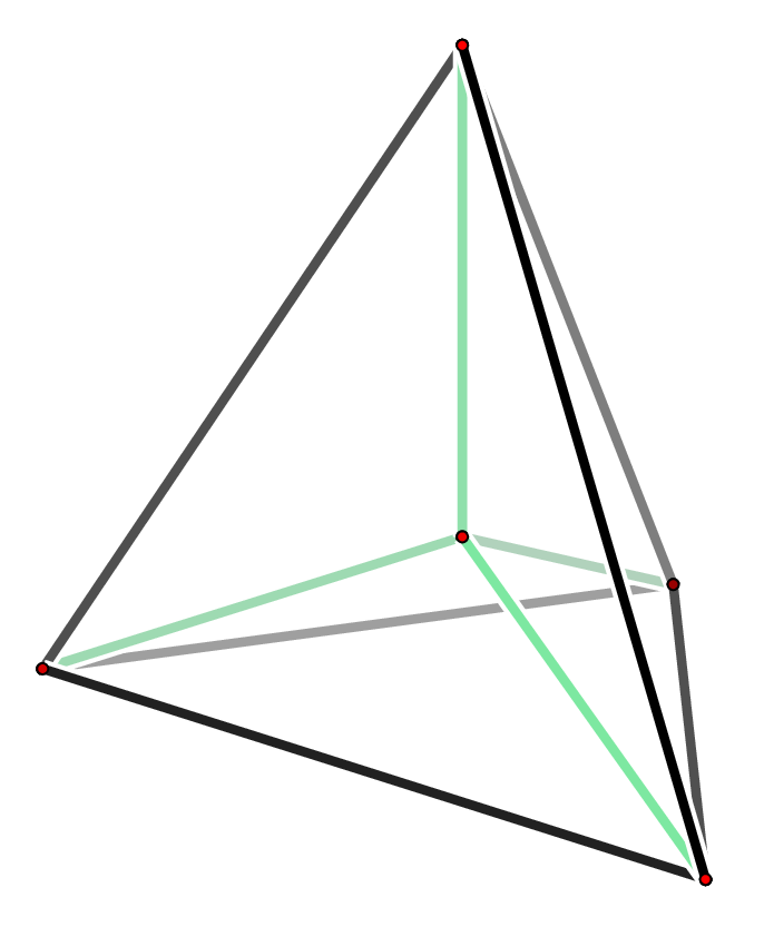


Example 3.2 (A cubical -polytope with the graph of a -cube [Z62]).
The construction
for a square such as , yields a -polytope whose Schlegel diagram is displayed in Figure 3.2. This polytope is cubical: All its facets are combinatorially equivalent to the -cube .
The -vector may be derived from the figure, but indeed it may also be deduced just from the information that this is a cubical -polytope with the graph of a -cube. (The latter yields and , the “cubical” property implies by double counting, and then there is the Euler–Poincaré equation [Z35, Sect. 8.2], which for -polytopes reads . See also Exercise 3.2.)

Example 3.3 (The hypersimplex).
The hypersimplexes form a -parameter family of remarkable polytopes; as Robert MacPherson said in his PCMI lectures, they have by far not received the attention, study, and popularity that they deserve. They do appear, for example, as in [Gr1-2, p.65], as in [GGL, Sect. 1.6] (where apparently the name “hypersimplex” appeared first), in [gelprimefand82:_geomet_grass], in [GKZ, p. 207], and in [LST]; but also elsewhere they appear under disguise, for example, as the cycle polytopes of uniform matroids (see e.g. [Groetschel2004b]).
The hypersimplex may be defined as the convex hull of all the -vectors of length that consist of ones and zeroes. This is a -dimensional polytope with vertices. In the special case and we obtain simplices.
What we call the hypersimplex is a -dimensional polytope that appears in this family. It may be defined, lying on a hyperplane in , as
or equivalently, after projection to by “deleting the last coordinate,” as
The first representation is more symmetric: It yields “by inspection” that all vertices of this polytope are equivalent (under symmetries that permute the coordinates), but that there are two types of facets, five simplices and five octahedra, which appear in vertex-disjoint pairs, “opposite to each other,” in parallel hyperplanes. In particular, all the facets are simplicial, that is, all the -faces are triangles, so the polytope is -simplicial.
The second representation has the advantage of being full-dimensional, and it supplies us with a Schlegel diagram (using an octahedron facet as a “window”), as displayed in Figure 3.3. In the figure we may see that the (ten, equivalent) vertex figures are triangular prisms, so they are simple; thus in this -polytope, each edge is in exactly three facets, so the polytope is -simple. So we have seen our first example (other than the -simplex) of a -simple, -simplicial -polytope.
From the data given it is easy to compute the -vector of the hypersimplex: It is .

3.2. -simple -simplicial -polytopes
Definition 3.4.
A -polytope is -simple -simplicial (“ss” for short) if all -faces of , and of , are triangles.
The definition given here has the nice feature of being self-dual: Clearly, is 2s2s if and only if its dual is 2s2s. A more explicit version is that a -polytope is 2s2s if and only if
-
every -face has the minimal number of vertices, and if
-
every -face (edge) lies in the minimal number of facets.
Still equivalently, this is if and only if
-
for every -face the lower interval in the face lattice of is boolean, and if
-
for every -face the upper interval in the face lattice of is boolean.
Thus the 2s2s property may be pictured in analogy with the properties of being simple, or being simplicial. For this we note that, for example, is simplicial if
-
for every -face (facet) the lower interval in the face lattice of is boolean, and if
-
for every -face (ridge) the upper interval in the face lattice of is boolean.
(The first property just says that the facets should be simplices; the second property is automatically satisfied: Every ridge lies in two facets.) And similarly for simple -polytopes — see Figure 3.4.
Of course all this suggests generalizations, to ask for -simple -simplicial -polytopes, apparently introduced by Grünbaum [Gr1-2, Sect. 4.5]. For these don’t exist (other than the -simplex), but also for small and they are hard to construct. Indeed, are there any -simple -simplicial -polytopes that are not simplexes? Not a single example is known. Compare [Z89] for more information. Here we will restrict ourselves to the -dimensional case of 2s2s polytopes. Let’s note one interesting property that is specific for the -dimensional case, and which also confirms the impression that 2s2s -polytopes form a “diagonal” case.
Lemma 3.5.
Every ss -polytope has a symmetric -vector: , .
Proof.
If is -simplicial, then each -face has three edges. Thus the number of incidences between -faces and edges, denoted , is . If it is -simple, then each edge lies in three -faces, that is, the number of indicences is . Combination of the two conditions forces . With this, Euler’s equation yields . ∎
This proof may be rephrased in terms of the face lattice: For -polytopes the 2s2s conditions force the two middle rank levels of the face lattice to form a bipartite cubic graph — which as any other regular bipartite graph has to have the same number of vertices on each shore. You should identify this bipartite cubical graph in the face lattice of the hypersimplex, as displayed in Figure 3.5, and thus verify the 2s2s property for this face lattice. The symmetry of the -vector is explained by Lemma 3.5; nevertheless, the hypersimplex and its face lattice are not self-dual: There are two types of facets, but only one symmetry class of vertices.

The fact that the dual of any 2s2s -polytope is again 2s2s (by definition), and the symmetry property for the -vector, might suggest that 2s2s polytopes live in some sense “between” simple and simplicial. This is not true, as we will see in the next lecture, when we locate their -vectors in the cone of all -vectors of -polytopes. Indeed, the 2s2s polytopes are so interesting because they form a class of extremal polytopes in terms of the flag vector: A -polytope is 2s2s if and only if the valid inequality
holds with equality. (Compare Exercise 3.7.)
3.3. Deep vertex truncation
The idea for “deep vertex truncation” is very easy: Cut off all vertices of a polytope — but don’t just truncate the vertices, but cut them off by “deep cuts,” that is, so deeply that exactly one point remains from each edge.
All that is said and done about “deep vertex truncation” in the following works and makes sense for . Nevertheless, the pictures will primarily represent the case , while the most interesting results appear for .
Definition 3.6 (Deep vertex truncation).
Let be a -polytope, .
A deep vertex truncation
of is obtained by cutting off all the vertices of (by closed halfspaces , one for each vertex ) in such a way that from each edge of , exactly one (relative interior) point remains.
Equivalently, a deep vertex truncation is obtained as the convex hull
of points placed on the edges of in such a way that for each vertex of , the points chosen on the edges adjacent to lie on a hyperplane .
It is quite obvious that a deep vertex truncation can be constructed for each simple polytope , but we will be particularly interested in the case of simplicial polytopes: For these it is not so clear that the cutting can be performed so that all constraints are satisfied simultaneously.
Lemma 3.7.
Every -polytope has a realization for which deep vertex truncation can be performed.
Proof.
Take an edge-tangent Koebe–Andreev–Thurston representation (according to Lecture 1). Then can be taken as the tangency points, and the cutting hyperplanes are spanned by the vertex horizon circles. ∎


For , every deep vertex truncation polytope has two types of facets:
-
deep vertex truncations of the facets of , and
-
the vertex figures of .
Proposition 3.8 (Paffenholz & Ziegler [Z89]).
If is a simplicial -polytope, then any deep vertex truncation is -simple and -simplicial.
Proof.
The two types of facets of are the octahedra , for the tetrahedron facets of , and the vertex figures of , which are simplicial. Thus -simplicial.
Since all edges of are reduced to points by deep vertex truncation, all the edges of are “new,” they arise by deep vertex truncation from the -faces (that is, the ridges) of . Each such ridge lies in two facets of , so the edge we are looking at lies in two facets and of the first type, and in one facet of the second type. Thus each edge of lies in exactly three facets, that is, is -simple. ∎
So we have that is 2s2s for any simplicial -polytope … if it exists. And that’s the problem: In general it is not at all guaranteed that deep vertex truncation can be performed. One would try to realize cyclic -polytopes in such a way that deep vertex truncations can be performed, but it seems that this is not possible. Similarly, if a sum is realized “the obvious way,” with regular polygons in orthogonal subspaces, then deep vertex truncation is not possible except for very special cases (such as ): It is quite surprising that the sums of polygons do have a realization such that deep vertex truncation is possible, as proved by Paffenholz [paffenholz-pc]. On the other hand, there does not seem to be a single example of a simplicial polytope for which it has been proved that deep vertex truncation is impossible for all realizations.
However, in special cases deep vertex truncation can indeed be performed. In particular, any regular polytope admits a deep vertex truncation — just take the edge midpoints for . From this we get the following three examples of 2s2s -polytopes:
-
Deep vertex truncation of a simplex, , yields the hypersimplex.
-
Deep vertex truncation of the -dimensional cross polytope,
yields Schläfli’s 24-cell (see Figure 3.7):
-
Deep vertex truncation of the regular 600-cell (which has 600 regular tetrahedra as facets) yields a 2s2s -polytope with 720 vertices, whose vertex figures are prisms over regular pentagons; its facets are 600 octahedra, and 120 regular icosahedra. It seems that this remarkable polytope, with -vector , first occured in the literature in 1994, as the dual of the “dipyramidal 720-cell” constructed by Gévay [Gevay]. See also Exercise 3.2.

3.4. Constructing
The stacked polytopes form an infinite family of simplicial polytopes which can quite easily be realized in such a way that deep vertex truncation can be performed.
For this, we denote by any combinatorial type of a -polytope, , which is obtained by times stacking a pyramid onto a simplex facet, starting at a -simplex. This is a simplicial -polytope with vertices and facets; see Exercise 3.3. Note that the notation “” does not specify a combinatorial type; many different types may be obtained by stacking onto different sequences of facets (cf. Exercise 3.6).
Theorem 3.9 (Paffenholz & Ziegler [Z89]).
Any combinatorial type of a stacked -polytope can be realized so that it admits a deep vertex truncation.
Proof.
We proceed by induction on , starting at , with a -simplex, and a deep vertex truncation that takes the convex hull of the edge midpoints.
Assume now that has been realized as such that can be obtained by a suitable choice of points on the edges . Assume that arises by stacking onto a facet of that is realized by the facet with vertex set . The “new” vertex is now chosen “beyond” the facet of , and “beneath” all other facets of . That is, addition of to would mean stacking a pyramid onto the facet of . In particular, lies “beyond” the facet of , and “beneath” all other facets of , so is a stacked polytope realizing , as required.
The facet hyperplanes of cut the edges of in points : This is since is beneath , while is cut off by . Thus we obtain points on the new edges of , and the hyperplane may be taken to cut off the new vertex of . This new truncation plane is determined uniquely by the intersection points, because the new vertex of is simple. ∎
This theorem is valid for all ; in particular, 3D-pictures work. (Figure 3.8 is a feeble attempt.) However, the construction produces by far the most interesting results for .
Corollary 3.10 ([Z89]).
For each , and for every type of stacked -polytope with -vector , there is a corresponding -simple -simplicial -polytope , with -vector
In particular, this yields infinitely many combinatorial types of -simple -simplicial -polytopes. Moreover, with a bit of care the proof of Theorem 3.9 yields these polytopes with rational vertex coordinates. See [Paffenholz:Webpage2s2s] for explicit examples of such coordinates.
Corollary 3.11 ([Z89]).
The number of combinatorial types of -simple -simplicial -polytopes with vertices grows exponentially in .
See Paffenholz & Werner [PaffenholzWerner:many] for further constructions of -simple -simplicial -polytopes with interesting -vectors. In particular, they describe the “smallest” example of such a polytope (other than the simplex), which has only vertices.
Exercises
- 3.1.
Show that any simple or simplicial -polytope with must be a simplex, or -dimensional.
- 3.2.
Compute the full -vectors, as well as the number of vertex-facet incidences, for the following -polytopes, based only on the information given here:
- (a)
The -cell: a 2s2s polytope whose facets are octahedra;
- (b)
The -cell: a simple polytope whose facets are dodecahedra;
- (c)
The -cell: a 2s2s -polytope whose facets are bipyramids over pentagons;
- (d)
A neighborly cubical polytope NCP, a cubical polytope with the graph of the -cube ().
- (a)
- 3.3.
Compute the full -vectors of the stacked -polytopes .
- 3.4.
Show that if a -polytope is not simplicial, then cannot be -simplicial.
- 3.5.
Find coordinates for . Check them with polymake.
(This is Braden’s “glued hypersimplex” [braden97].) - 3.6.
Show that there are exponentially many distinct combinatorial types of stacked -polytopes with vertices, for any . Derive that there are exponentially many types of -simple -simplicial -polytopes with the same -vector.
- 3.7.
Show that , and dually , holds for the flag vector of each -polytope.
(Hint: Sum the Euler equations for the facets, which are -polytopes.)
Derive from this that the inequality is valid for all -polytopes, and that it is tight exactly for the -simple -simplicial -polytopes. - 3.8.
Show that there is no -vector inequality (not involving ) that characterizes the 2s2s -polytopes.
- 3.9.
If is a -dimensional simplicial polytope, and if exists, is then -simple? -simplicial?
Gr1-2
f-Vectors of 4-Polytopes
The -vector of a -polytope is a quadruple of integers , but due to the Euler-Poincaré relation the set of all -vectors of -polytopes is a -dimensional set: It lies on the “Euler-Poincaré hyperplane” in , given by
The task we are facing is to describe the set of all -vectors,
Here “describe” may mean a number of different things: Probably one should not hope for a complete description (as Steinitz got for the -dimensional case), since the set of -vectors is way more complicated in the -dimensional case.
Indeed, is not the set of all integral points in a polyhedral cone, or even in a convex set. This may be seen from the characterizations of the projections of to the coordinate -planes in , by Grünbaum, Barnette, and Reay [\, Sect. 10.4
[barnette74:_e_s] [barnette73:_projec], which show non-convexities and holes (see Figure ). Or you just note that some of the rather basic, tight inequalities, such as the upper bound inequality , are concave. For example,
The midpoint of the segment between and is the integral point : It violates the upper bound inequality, and indeed a -polytope with vertices cannot contain more than the edges. (See also Bayer [Bay], Höppner & Ziegler [Z59].)
center
In the following, we will head for a complete description of the $f$-vector cone for $4$-polytopes, $cone(F_4)$. This seems to be a challenging but realistic goal. Once that is achieved (the ``2006 project''), a logical next goal might be a description of the ``large'' $f$-vectors, that is, of
for some large~$M$. But let's not get too ambitious too fast.
4.1. The $f$-vector cone
Definition 4.1 ($f$-vector cone).
The $f$-vector cone of $4$-polytopes, $cone(F_4)$, is the topological closure of the convex cone with apex $f(Δ_4)=(5,10,10,5)$ that is spanned by the $f$-vectors of $4$-polytopes,
Equivalently, $cone(F_4)⊂R^4$ is the solution set to all the linear inequalities that are valid for all $f$-vectors for $4$-polytopes, and that are tight at the $f$-vector of the simplex.
The equivalence between the two versions of the definition rests on basic facts about closed convex sets, which you should put together yourself (Exercise 4.1). You are also asked to verify that the cone generated by the $f$-vectors is not closed, so we do have to take the topological closure (Exercise 4.2.)
The closed convex cone we are looking at is $3$-dimensional, so we may view it as the cone over a $2$-dimensional convex figure, which might be just a pentagon or hexagon. Instead of looking at a $2$-dimensional section (say intersecting by $f_1+f_2=100$), we may equivalently introduce homogeneous (``projective'') coordinates, which are rational linear functions, normalized to yield ``$ 0 0 $'' at the $f$-vector of a simplex (compare Lecture~1). There is no unique best way to do this; we choose
as our homogeneous coordinates. (Figure~4.2 illustrates the geometry of such a rational function on a cone.) So we are trying to describe $proj(F_4)⊂R^2$, the closure of
Any $4$-polytope yields a (rational) point in the $(φ_0,φ_3)$-plane. Any valid linear inequality, tight at the $4$-simplex, translates into a linear inequality in $φ_0$ and~$φ_3$. So let's look at some families of polytopes and of linear inequalities that we know, and let's see what they buy us.
Some 4-polytopes we know:
|
The truncated polytopes are the duals of the stacked polytopes, so they are simple. Similarly, the duals of cyclic polytopes are simple. Thus we find the four points $( 1 10 , 3 10 )$, $( 3 10 , 1 10 )$, $(0, 1 3 )$, and $( 1 3 , 0 )$, which span a quadrilateral subset of $proj(F_4)$. This quadrilateral also represents the $f$-vectors of simple and of simplicial polytopes and ``everything in between.'' (Note that duality interchanges the coordinates $φ_0$ and~$φ_3$, and thus $proj(F_4)$ is symmetric with respect to the main diagonal.)
Five linear constraints we know:
|
The first four inequalities are quite trivial, and we have named them by the polytopes that satisfy them with equality, at least asymptotically. The translation into $(φ_0,φ_3)$-inequalities, using the Euler-Poincaré relation, poses no problem. There is no polytope with $φ_0=0$, but the condition is satisfied asymptotically by any family of $4$-polytopes with far more vertices than facets. For example, the products of $n$-gons, with $f(P_n×P_n)=(n^2,2n^2,n^2+2n,2n)$, yield $(φ_0,φ_3)=( n^2-5 3n^2+2n-20 , 2n-5 3n^2+2n-20 ) ∈proj(F_4)$, which in the limit $n→∞$ yields $( 1 3 ,0)$.
The one non-trivial inequality in our table above is the last one, a ``Lower Bound Theorem.'' It may be derived quite easily [Bay] from the inequality $f_03≥3f_0+3f_3-10$, which was first established by Stanley [Sta7] in terms of the so-called toric $g$-vector (it is the inequality ``$g_2^tor(P)≥0$''); a proof via rigidity theory was later given by Kalai~[kalai87:_rigid_i].
Figure~4.3 summarizes our discussion up to this point: We are interested in~$proj(F_4)$, the closure of the set
This set is contained in the pentagon cut out by the five linear inequalities discussed above, and it contains the shaded trapezoid, which represents ``everything between simple and simplicial polytopes.'' Indeed, simple and simplicial polytopes satisfy the additional linear inequality $φ_0+φ_3≥ 1 3 $.
Thus we are left with the following ``upper bound problem'':
``Upper Bound Problem''.
Are there $4$-polytopes with $φ_0+φ_3→0$ ?
The inequality $φ_0+φ_3≥ 1 3 $ is certainly not valid for all (possibly non-simple non-simplicial) $4$-polytopes: Already for the hypersimplex we get $(φ_0,φ_3)=( 1 8 , 1 8 )$.
However, currently it is not clear how small $φ_0+φ_3$ can be for convex polytopes. Thus the Upper Bound Problem is the key remaining problem in the description of the $f$-cone for $4$-polytopes.
- ˜(!)˜
If the answer is YES to the problem as posed above, then the five inequalities above constitute a complete linear description of~$cone(F_4)$.
- ˜(!)˜
If the answer is NO, then this is also exciting, since it means that the answers for cellular spheres and for convex polytopes are distinct! Indeed, cellular $3$-spheres with arbitrarily small $φ_0+φ_3$ have been constructed by Eppstein, Kuperberg & Ziegler [Z80]; see our discussion in Section~4.3.
4.2. Fatness and the Upper Bound Problem
We prefer to rephrase the Upper Bound Problem in terms of a somewhat more graphic quantity, which we call ``fatness.''
Definition 4.2 (Fatness).
The fatness of a $4$-polytope is the quotient
The fatness of a $4$-polytope is large if both $φ_0$ and~$φ_3$ are small. This happens if the polytope has relatively few vertices and facets, but many edges and $2$-faces. Thus, graphically, the face lattice and the $f$-vector are ``fat in the middle,'' whence the name (see Figure~4.4).
``Upper Bound Problem''.
Can the fatness of a $4$-polytope be arbitrarily large?
Here are a few explicit values to start with: For stacked and truncated $4$-polytopes we have $F(P)= 5 2 $ exactly. For cyclic polytopes we get $F(C_4(n))→3$ for $n→∞$, and the same for the duals — fatness is a self-dual quantity, that is, any $4$-polytope and its dual have the same fatness. Moreover, it is easy to compute (or to derive from Figure~4.3) that all simple and simplicial polytopes satisfy $ 5 2 ≤F(P)<3$.
But how large can fatness be? The attempts to answer this question have led to a multitude of interesting examples and constructions, and to a fast succession of record holders for ``the fattest examples found so far.'' Many of them can be obtained by deep vertex truncation of simplicial polytopes, so they are $2$-simple and $2$-simplicial by Proposition~3.8:
- –
The hypersimplex, which is the dual of $DVT(Δ_4)$, has fatness $4$.
- –
Schäfli's $24$-cell [Schla], $DVT$(cross polytope), has fatness~$4.526$.
- –
Gévay's $720$-cell~[Gevay], the dual of $DVT$($120$-cell), has $720$ facets that are bipyramids over regular pentagons. It has fatness~$5.020$.
- –
Eppstein, Kuperberg & Ziegler [Z80] used hyperbolic geometry arguments to achieve a fatness of~$5.048$ by the ``E-construction,'' which is dual to deep vertex truncation.
- –
Paffenholz [paffenholz-pc] has very recently shown that there are realizations for any sum of an $n$-gon and $m$-gon such that the deep vertex truncation $DVT(P_m×P_n)$ can be obtained. For $m=n→∞$ this yields fatness approaching~$6$.
However, we'll go a different route. In the next and final lecture we will present a construction that generalizes and extends the construction of ``neighborly cubical'' $4$-polytopes of Joswig & Ziegler~[Z62], to achieve fatness arbitrarily close to~$9$, the latest record (as far as I know at the time of writing). I would have been happy to have a ``note added in proof'' about this~…
What do polytopes ``of very high fatness'' look like? You can verify (via Exercise 4.6) that they have two properties:
- ˜(1)˜
The facets have many vertices (on average).
- ˜(2)˜
The vertices are in many facets (on average).
Either of these properties are easy to satisfy — just look at the products $P_n×P_n$ for the first property, and at their duals, the free sums $P_n⊕P_n$, for the second one. The key question is whether they can simultaneously be satisfied.
Finally, here is a problem on $3$-dimensional polytopal tilings that is ``essentially'' equivalent to the fatness problem: Consider face-to-face tilings of~$R^3$ (cf.~[SchattschneiderSenechal]) that satisfy some regularity properties, e.g. one of the following (each implies the next):
- ˜–˜
the tiling is triply periodic (that is, there are three linearly independent translational symmetries),
- ˜–˜
there are only finitely many distinct congruence classes of tiles,
- ˜–˜
in- and circumradius of the tiles are uniformly bounded.
For such tilings, we may define notions of ``average'' vertex degrees, face numbers, etc. The question is whether there is such a tiling where the tiles have lots of vertices on average, and the vertices are in many tiles on average. Again, either property is easy to achieve (look at tilings by Schlegel diagrams), but can they be simultaneously satisfied?
4.3. The Lower Bound Problem
The upper bound problem discussed here has a natural ``lower bound'' counterpart. It arises if we don't restrict ourselves to the geometric model of convex polytopes, but consider the larger class of cellular spheres that are ``regular'' in the sense that their cells have no identifications on the boundary, and that satisfy the ``intersection property'' that any two faces should intersect in a single cell (which may be empty). These are the regular CW spheres [CookeFinney] whose face poset is a lattice (where the meet operation corresponds to intersection of faces).
``Lower Bound Problem''.
Does $φ_0+φ_3≤ 2 5 $ hold for the cellular spheres that satisfy the intersection property?
This problem seems crucial in terms of the separation of the ``geometric'' model of convex polytopes from the ``topological'' model of cellular spheres/balls.
- ˜(!)˜
If the answer to the problem is NO, then this would establish such a separation, which would be quite remarkable.
- ˜(!)˜
If the answer is YES, then this would imply a complete characterization of the $f$-vector cone for cellular $3$-spheres, by the five linear inequalities given above; indeed, Eppstein, Kuperberg & Ziegler [Z80] have constructed cellular spheres for which fatness is arbitrarily large, that is, $φ_0+φ_3$ is arbitrarily small.
We will not discuss this here further, but refer to [Z80] and~[Z82].
Exercises
- 4.1.
Show that the two definitions of the $f$-vector cone given in Definition~4.1 are indeed equivalent.
Hint: You need a separation lemma; see for example Matoušek~[matousek02:_lectur_discr_geomet, p.~6]. - 4.2.
Show that the union of the line segments $[f(Δ_4),f(C_4(n))]⊂R^4$ has the whole ray ${(5,10+t,10+2t,5+t):t≥0}$ in its closure. Note that $f_0≥5$ is a valid linear inequality, which is tight at $f(Δ_4)$, but for no other $f$-vector.
Conclude that the cone with apex $f(Δ_4)$ spanned by the $f$-vectors of $4$-polytopes is not closed. - 4.3.
Compute the fatness and the $(φ_0,φ_3)$-pair for the hypersimplex, the $24$-cell, and for $DVT(600$-cell).
- 4.4.
Compute the fatness of the 2s2s polytopes $DVT(Stack(n,4))$, and show that it lies in the interval $[4, 4.5)$.
Show that for any simplicial $4$-polytope $P$, the fatness of $DVT(P)$ is smaller than~$6$.
Where would the $f$-vectors of the polytopes $DVT(P)$ lie in $proj(F_4)$, as graphed in Figure~4.5? - 4.5.
If $C^n_4$ is a cubical $4$-polytope with the graph of an $n$-cube (see Exercise~3.2), compute the fatness and the pair $(φ_0,φ_3)$.
- 4.6.
Define the complexity of a $4$-polytope to be the quotient
- (a)
Show that $F(P)≤2C(P)-2$, with equality if and only if $P$ is $2$-simple and $2$-simplicial.
- (b)
Show that $C(P)≤2F(P)-2$, with equality if and only if if all facets of~$P$ are simple, or equivalently, if all vertex figures are simple.
- (c)
Derive from this that fatness is high if and only if both the average number of vertices per facet, $f_03/f_3$, and the average number of facets per vertex, $f_03/f_0$, are large.
- (a)
Projected Products of Polygons
In this lecture we present a construction of very recent vintage, ``projected products of polytopes.'' We will not have the ambition to work through all the technical details for this; these appear in~[Z97], see also [Z102]; rather, our main objective is here to identify the structural features of the construction which lead to fat polytopes, and to outline (possibly ``for further use'') some interesting components that go into the construction. In the following version of the main result, some concepts that will be explained below are highlighted by quotation marks.
Theorem 5.1 (Ziegler~[Z97]).thm:PPP
For each $r≥2$, and even $n≥4$, there is a realization
$P^r_n⊂R^2r$ of a product of polygons $(P_n)^r$ (a
``deformed product of~polygons'') such that the vertices and edges
and all the ``$n$-gon $2$-faces'' of~$P^r_n$ ``survive'' the
projection $π:R^2r→R^4$ to the last $4$ coordinates.
A number of nice tricks go into the
construction that proves the theorem — see below.
Before we look into these we want to derive the enumerative consequences:
The $f$-vector of~$π(P^r_n)$ can be derived purely from the information
given in the theorem, not using details about the combinatorics
of the resulting polytopes (which were worked out only
recently [dipl-Sanyal] [Z102]).
5.1. Products and deformed products
We have discussed the construction and main properties of
products of polytopes already in Example~2.7.
A key observation is that the non-empty faces of a product are
the products of non-empty faces of the ``factors.''
Now we specialize to the case of products of (several) polygons:
We consider products of~$r$ $n$-gons — and later we
will be looking at polytopes that just have the combinatorics
of such polytopes.
If $P_n$ is an $n$-gon, then $(P_n)^r$ is a simple polytope
of dimension $2r$.
It has
~$∙$~
5.1. Products and deformed products
We have discussed the construction and main properties of products of polytopes already in Example~2.7. A key observation is that the non-empty faces of a product are the products of non-empty faces of the ``factors.'' Now we specialize to the case of products of (several) polygons: We consider products of~$r$ $n$-gons — and later we will be looking at polytopes that just have the combinatorics of such polytopes. If $P_n$ is an $n$-gon, then $(P_n)^r$ is a simple polytope of dimension $2r$. It has ~$∙$~thm:PPP For each , and even , there is a realization of a product of polygons (a ``deformed product of polygons'') such that the vertices and edges and all the ``-gon -faces'' of ``survive'' the projection to the last coordinates.
$f_0=n^r$ vertices (of the form ``vertex $×$ vertex $×$ ………$×$ vertex''), and
$f_1=rn^r$ edges (of the form ``vertex $×$ …$×$ edge $×$ …$×$ vertex). The products of polygons have two different types of $2$-faces, ``quadrilaterals'' and ``polygons,'' that we need to distinguish:
- ˜$∙$˜
$ ( r 2 ) n^r$ quadrilateral $2$-faces (which arise as products of two edges, and vertices from the other factors), and
- ˜$∙$˜
$rn^r-1$ polygon $2$-faces (arising as a product of one $n$-gon factor with vertices from the other factors).
Thus we get $f_2=
