A Variational Principle Based Study of KPP Minimal Front Speeds in Random Shears
Abstract
Variational principle for Kolmogorov-Petrovsky-Piskunov (KPP) minimal front speeds provides an efficient tool for statistical speed analysis, as well as a fast and accurate method for speed computation. A variational principle based analysis is carried out on the ensemble of KPP speeds through spatially stationary random shear flows inside infinite channel domains. In the regime of small root mean square (rms) shear amplitude, the enhancement of the ensemble averaged KPP front speeds is proved to obey the quadratic law under certain shear moment conditions. Similarly, in the large rms amplitude regime, the enhancement follows the linear law. In particular, both laws hold for the Ornstein-Uhlenbeck process in case of two dimensional channels. An asymptotic ensemble averaged speed formula is derived in the small rms regime and is explicit in case of the Ornstein-Uhlenbeck process of the shear. Variational principle based computation agrees with these analytical findings, and allows further study on the speed enhancement distributions as well as the dependence of enhancement on the shear covariance. Direct simulations in the small rms regime suggest quadratic speed enhancement law for non-KPP nonlinearities.
1 Introduction
Front propagation in heterogeneous fluid flows has been an active research topic for decades (see [7], [17], [14], [23], [24], [25], [27] and references therein). A fascinating phenomenon is that the large time (large scale) front speed can be enhanced due to the presence of multiple scales in fluid flows. Speed characterizations and enhancement laws have been studied mathematically for various flow patterns by analysis of the proto-type models, e.g. the reaction-diffusion-advection equations (see [3, 5, 8, 12, 15, 17, 18, 19, 21, 22, 24, 25, 26] and references therein). The enhancement obeys a quadratic law in the small amplitude flow regime, known as the Clavin-Williams relation [7], which is proved to be true for deterministic shear flows [22], [12], [20], [21] etc. The enhancement is proved to grow linearly in large amplitudes of deterministic flows (shear and percolating flows), see [4, 8, 11, 15, 20, 21] etc. However, enhancement exponent 4/3 was reported based on numerical simulation of random Hamilton-Jacobi models (so called G-equation or KPZ model) on fronts in weak randomly stirred array of vortices [15]. Likewise, formal renormalization group method [27] suggested that front speeds may grow sublinearly (slower than linear by a logarithmic factor) in the strong random flow regime. These two findings raised the issue as to what extent the speed enhancement laws in the deterministic flows are valid for random flows. Recently, one of the present authors [26] showed that both the quadratic and linear laws hold almost surely for Kolmogorov-Petrovsky-Piskunov (KPP) minimal front speeds through white in time spatially Gaussian random shears on the plane. Yet the KPP front speeds diverge almost surely in spatially Gaussian random shears. A powerful tool is the variational principle of KPP minimal front speeds.
In this paper, we consider KPP front speeds through random shear flows in channel domains , where , , a bounded simply connected domain with smooth boundary. We shall address the enhancement laws of the ensemble averaged front speeds. The model equation is:
| (1.1) |
where , the -dimensional Laplacian, . The nonlinearity , the so called KPP reaction. Other nonlinearities [25] will be discussed later. The vector field where is a stationary continuous scalar random process in , its ensemble mean equal to zero. The zero Neumann boundary condition is imposed at : , the unit outward normal.
For nonnegative initial data approaching zero and one at infinities rapidly enough, the KPP solutions propagate as fronts with speed given by the variational principle [6, 25, 5]:
| (1.2) |
where is the principal eigenvalue with corresponding eigenfunction of the problem:
| (1.3) | |||||
| (1.4) |
The variational speed formula (1.2) makes possible an analysis of ensemble averaged random front speeds. Using variational formulas on the principal eigenvalue , we are able to obtain tight upper and lower bounds on and estimate in terms of moments of suitable norms of the shear over . For small root mean square (rms) shear, the quadratic enhancement law is proved and is explicit in case of the Ornstein-Uhlenbeck (O-U) process when . The linear growth law holds in the large rms regime under weaker moment conditions on the shear. In both regimes, the moment conditions are satisfied by the O-U process when .
The variational formula (1.2) also offers an efficient and accurate way to compute a large ensemble of random front speeds. Directly solving the original time dependent equation (1.1) to reach steady propagating states can be both slow and less accurate. Numerical difficulties abound for direct simulations due to three large parameters. A large ensemble of random fronts requires a large enough truncated channel domain to contain the front over large times. Due to occasional random excursions in , the domain size in has also to be made adaptively large. This can be prohibitively expensive in the regime of large rms shears.
The variational formula (1.2) allows us to compute quickly and accurately the ensemble averaged speeds in both small and large shear rms regimes when . An interesting difference from the deterministic case is that the integral average of in , i.e. , is a random constant not equal to zero. This quantity can be of either sign, and influence greatly the numerical approximation of in the small rms regime, even though it does not contribute to the exact , since . To assess the speed enhancement accurately, we subtract this random constant from each before evaluating the expectation numerically. This way, we are able to minimize the errors in approximating in a finite ensemble. In our computation, is a discrete O-U process.
In complete agreement with analysis, we find numerically that the ensemble averaged speeds obey a quadratic law in the small rms regime and a linear law in the large rms regime. Without the subtraction technique, the computed average speed enhancement in the small rms regime can give inaccurate scaling exponents significantly below two. The same technique and direct simulations for other nonlinearities (combustion, bistable) suggest quadratic speed enhancement in the small rms regime. The computed speed ensemble then permits us to study further the enhancement distribution and its dependence on variation of shear covariance functions.
The paper is organized as follows. In section 2, we prove the enhancement laws of ensemble averaged speeds based on variational principles, and derive a closed form speed asymptotic formula in case of O-U process. In section 3, we describe numerical methods for computing speed ensemble with the variational formula (1.2) and speed statistics, then show numerical results. We also make comparisons with the prediction of the asymptotic formula and with direct simulations. In section 4, we conclude with a remark on future works.
2 Average Speed Asymptotics
Consider scaling shear amplitude , and denote by the minimal KPP speed corresponding to shear . Let denote the minimal speed in case of zero advection. If the shear has zero integral average over , the corresponding minimal speed is always enhanced by the shear. This is true also for time dependent shears, see [21, 20] and references therein. For each realization, as ; as . For each realization, as , we have:
Proposition 2.1
Let solve , , with zero Neumann boundary condition, where , has zero mean over . Then for sufficiently small, the minimal speed has the expansion
| (2.5) |
Up to , the formula (2.5) is independent of the nonlinearity, see [22, 12] for being bistable or combustion nonlinearity, also [21] for more general nonlinearities and time periodic shears. We shall give a proof of Proposition 2.1 using variational formulas, and later generalize it to the random case. A helpful fact is that the infimum in (1.2) can be restricted to a bounded set independent of and , as stated in the following lemma:
Lemma 2.1
Let have zero mean over , and let . Then
| (2.6) |
Proof of lemma: For each , we let . So, if is the eigenfunction defined by (1.3), then is the principal eigenvalue defined by the equation
| (2.7) |
One can readily verify that . The variational formula (1.2) can be expressed as
| (2.8) | |||||
Consider the points where . By Proposition 2.1 of [6], the continuous curve is convex in , for each . Also, . Therefore, for a given , there can be at most two values of such that . The line satisfies , with equality holding only at one point: . Since and is convex and is a line, for some only if for some . This point is illustrated in Figure 1. The solid curve represents the parabola . If intersects , then one of the intersection points must be to the left of . Therefore, from (2.8),
| (2.9) |
So, we conclude that
| (2.10) |

Proof of Proposition 2.1:
To estimate , we bound the principal eigenvalue using two different representations of . First, since is a self-adjoint operator, we have:
| (2.11) |
where the supremum is taken over all such that on . The other representation is:
| (2.12) |
where the infimum can be taken over all such that , , and on . This representation follows from the fact that the eigenfunction lies in the kernel of the self-adjoint operator . So, if we have the strict inequality
| (2.13) |
then the Fredholm alternative implies that , a contradiction since , . Hence,
| (2.14) |
Since , the formula (2.12) follows. Note that we do not require the test functions to be , only . This is important since we do not want to require the shear to be any more regular that .
Let us derive upper and lower bounds for by choosing test functions as:
| (2.15) |
where and solve
| (2.16) |
with zero Neumann boundary conditions at , and a constant equal to:
| (2.17) |
We normalize and so that:
| (2.18) |
Then
and
| (2.19) |
Using the definition of , we see that , and
Now from (2.11) and (2.19) we have the lower bound
| (2.20) |
with
| (2.21) |
By choice of and , we have for all and . Hence, for bounded. Returning to the variational formula (2.10), we now have a lower bound on :
| (2.22) | |||||
To obtain an upper bound on , we use (2.12) and calculate:
| (2.23) | |||||
Since and , we see from (2.12) and (2.23) that
| (2.24) |
with
| (2.25) |
The variational formula (2.10) implies:
| (2.26) | |||||
completing the proof.
When the shear is a random process, the corresponding minimal speed is a random variable for each , and we consider how the expectation scales with the parameter by finding an exponent such that . Each realization of the process restricted to the domain does not necessarily have zero integral over . Nevertheless, each realization can be written in the form
| (2.27) |
where is the mean of over , and is the variation about the mean value. For a fixed realization, the minimal speed will be affected by both the scaling of the mean and the scaling of the varation . That is,
| (2.28) |
where the remainder is the enhancement due to the variation , different for each realization. Taking the expectation of both sides of (2.28), we have
| (2.29) |
For each sample, is for small. Though might exhibit different scaling than quadratic, we show that the quadratic scaling law remains for enhancement of averaged front speeds under suitable moment conditions of the shear.
Theorem 2.1
Let be a stationary random process in () so that sample paths are almost surely continuous; and that
| (2.30) |
Then for small, the expectation has the expansion
| (2.31) |
where ; and solves , subject to zero Neumann boundary condition.
Proof: As the contribution of to is just an additive constant, it suffices to consider shear flow and show that it gives the averaged speed
| (2.32) |
We adapt the proof of Proposition 2.1, noting however that in the stochastic case the remainders and defined by (2.21) and (2.25) are random and not bounded uniformly for all realizations. Instead, we will show that for in a bounded interval,
To this end, we estimate and , with denoting a generic positive constant depending only on the domain and its dimension. Let and solve (2.16) with . Applying estimates (e.g. Thm. 19.1 of [9]), we have
| (2.33) |
and
| (2.34) | |||||
since
| (2.35) |
Given , we can choose sufficiently large, depending on , such that embeds continuously into . It follows that there is a constant independent of such that
| (2.36) |
If instead we normalize and by (2.18), then the bounds (2.36) still hold, with different constants. Note that adding a constant to and does not alter the quantity that appears in the asymptotic expansion.
Since and are nonnegative, , for any realization. So for in a bounded interval and small, we bound (2.21) by:
so that
To bound , we use the normalization (2.18) and the above estimates:
| (2.37) |
Hence for in finite interval. Now we return to (2.22) to conclude
since ,
The opposite inequality follows from (2.26) since for . Thus formula (2.32) holds. For general , not necessarily mean zero,
The proof is finished.
In our numerical computation on front speeds in two dimensional channels, we use the Ornstein-Uhlenbeck (O-U) process for shear , so . Let us show below that the O-U process, denoted by , satisfies the conditions in Theorem 2.1, and so scales quadratically with for small.
Corollary 2.1 (Explicit Average Speed Formula)
Consider the O-U
process as solution of the Ito equation:
| (2.38) |
where is the standard Wiener process, is a Gaussian random variable with mean zero, and variance . Then satisfies the moment conditions in Theorem 2.1. The averaged KPP front speed in the channel is given by
| (2.39) |
where:
Proof: The O-U process is stationary and Markov. Its sample paths are almost surely Hölder continuous though nowhere differentible. The process can be written as
| (2.40) |
The covariance function of this process is . Letting denote the process
| (2.41) |
we see that is a martingale [13]. By Doob’s martingale moment inequality [13], for any ,
| (2.42) |
Since the process is Gaussian, (2.41) and (2.42) imply that
| (2.43) |
Formula (2.39) now applies to the average speed. Notice that
and
| (2.44) |
Let us calculate in terms of . Define:
so that
Thus
Now, we have
where denotes the average of over the interval , for . Consequently, we have
Using the O-U covariance function, we proceed as:
and
Letting , we have
Similarly,
Combining the above, we have
In view of (2.39), the proof is complete.
Theorem 2.2 (Linear Growth)
If the stationary shear process has almost surely continuous sample paths and satisfies , then the amplified shear field generates the average front speed:
Moreover, exists.
Proof: By Theorem 5.1 of [4], as , where is finite for each . Now recall the upper bound . Hence for , , and . The dominated convergence theorem implies that:
The proof is finished. Clearly, the O-U process satisfies the required condition for linear average speed growth.
3 Computation by Variational Principle
3.1 Numerical Methods
Let . For a given , we compute the principal eigenvalue with corresponding eigenfucntion , , by solving:
| (3.1) |
using a standard second order finite-difference method. Here we suppress the random parameter , as computation is done realization by realization. Denote the uniform partition of the domain by points , and the numerical solution by , where , , and . The discretized system is
with second order approximation of the Neumann boundary conditions. This reduces to finding the principal eigenvalue of a symmetric tridiagonal matrix, easily accomplished with double precision LAPACK routines [2]. Then we compute points on the curve , and minimize over using a Newton’s method with line search. Our approximation decreases with each iteration and converges quadratically in the region near the infimum. Two illustrative curves are shown in Figure 2 for two different realizations of the shear.

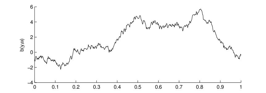
We generate realizations of the shear process by numerically evaluating the stochastic ODE (2.38) with the Milstein scheme (see [16]). Although this scheme is first order, we use a discrete spacing , where is the discrete grid spacing for the eigenvalue problem, so that the method is still second order accurate in the parameter . Figure 3 shows a sample path, and Figure 4 compares exact and numerical covariance function constructed from 5000 samples.

To approximate the expectation we generate independent realizations (indexed by ) of the shear and compute the corresponding minimal speeds for each . Then we compute the average
| (3.2) |
where . That is, we subtract the linear part due to the mean of the shear being nonzero, as in (2.28).
Once we have the averages for each , we compute the exponents using the least squares method to fit a line to a log-log plot of speed versus amplitude. That is, the exponent is the slope of the best-fit line through the data points for each shear amplidute .
3.2 Numerical Results
3.2.1 Scaling with shear amplitude
In Figure 5 and Figure 6, we show the results of a simulation using realizations of a shear in small and large root mean square (rms) amplitudes, respectively. As shown later in Figure 11, we find that the choice of samples was more than enough to obtain good convergence of the speed distribution functions. The covariance function of the process is . In each plot, we show multiple curves, corresponding to various domain sizes. In Figure 5, corresponding to small , the solid curves are the numerically computed values; the dashed curves are given by formula (2.39). We find that the enhancement of the minimal speed scales quadratically for small amplitudes and linearly for large amplitudes. The computed exponents are shown in Table 1.

As an application of the numerical results for large amplitudes, we compare the distribution of with the distributions of the random variables and , where is the diffusion constant (equal to 1 in equation (1.1)). Theorem 2 of [11] shows the upper bound:
| (3.1) |
and provided that is sufficiently small, depending on the realization. In Figure 7 we compare the distributions for , , and for . The asymmetry is seen in all three curves.


3.2.2 Dependence on Covariance
Next, we consider the effect of the covariance on the enhancement of the minimal speed. The covariance is a function of , so we will write . By choosing , we constructed O-U processes with covariances given by
| (3.2) |
By this choice of , the norm of remains constant as changes, so that the total energy in the power spectrum of the signal remains constant. Since , we see from equation (2.39) that for fixed ,
| (3.3) |
and that achieves a maximum for some finite value of . This suggests that there is some optimal , depending on the domain size , such that the enhancement of is maximized.
Fixing the grid spacing , we computed the expected value for a range of and for . Note that for each , we must choose the initial points to have variance so that the process remains stationary for each . Varying the covariance does not effect the order of the scaling in . That is, in each case the enhancement scales like for small and for large , as in the preceding simulation.
Figure 8 shows the enhancement for a fixed and a range of . Figure 9 shows the results of the same computation for , corresponding to the large regime. In this case, formula (2.39) is no longer valid. Nevertheless, we see the same effect as in the small amplitude regime: the existence of an optimal covariance parameter .


This effect can be interpreted in terms of and its Fourier transform or power spectrum:
| (3.4) |
As , concentrates at the origin, and so the energy of the shear process is concentrated more in the large scale spatial modes. The domain , to which the process is restricted, is bounded, and variations over a length scale that is much greater than the diameter of have little effect on the average enhancement of the front. As a result, decreases as . In the other limit , spreads out so that the energy over any finite band of frequencies goes to zero, causing to decrease as well. Note that in as , so even though spreads out more uniformly as , the family of processes does not converge to white noise, whose covariance function equals the Dirac delta function.
3.2.3 Speed Distribution
For a fixed and (corresponding to small and large amplitudes), we computed the distributions of the numerically computed values . The distributions are shown in Figure 10. To compute these distributions, we partition the range of values into disjoint intervals: . Then, we let
| (3.5) |
where is the characteristic function of the interval . The distributions in Figure 10 were computed with samples, and .
The values are the enhancement of the minimal speeds due to the variation of the shear, after the effect of the mean field has been subtracted off. Since a mean zero shear always enhances the minimal speeds, we should expect for all , for all realizations. As already noted, Figure 11 shows good convergence of the distributions when using samples.


3.2.4 Comparison with Direct Simulation
When comparing the results of the previous sections with results from direct simulation, we find that computing the minimal speeds using the variational formula offers significant advantages. As in [21], we first computed the quantities via direct simulation of the original equation (1.1) on a truncated domain using an explicit second-order upwind finite difference scheme. We chose the diffusion constant in the direct simulations to be and the grid spacing to be , . For each realization of the shear, we evolved the solution of (1.1) for a sufficiently long time until the front moves at a more or less constant speed (see [21] for details of the method). In this way, we approximated the minimal speed for each realization; then, we repeated the process for a large ensemble of shears to compute the expectations .
We considered three nonolinearities in our direct simulations:
- •
KPP nonlinearity: .
- •
Combustion nonlinearity: for , and for , for some . Also, .
- •
Bistable nonlinearity: for some .
Although there is no known variational formula as simple as formula (1.2) for the bistable and combustion nonlinearities, the expansion (2.5) holds for each of the nonlinearites (see also Theorem 4.2 of [12]). Therefore, we should expect that for small , the computed values
| (3.6) |
have approximately the same distribution, independent of the nonlinearity. For each nonlinearity, we computed more than 700 realizations of the shear and evolved the solution, as described in [21]. A relatively smaller number of samples was due to the long time required to compute each sample (not a problem with the variational formula in the KPP case). After subtracting off the linear part of the enhancement (due to mean field), we computed the enhancement exponent as described in Section 3. The results of the direct simulation concur that, for small amplitudes, scales like . Figures 12, 13, and 14 show the distributions of the computed values for the KPP, combustion, and bistable nonlinearities, respectively, for . We see that the distributions are roughly the same, independent of the nonlinearity, as should be expected. While computationally expensive, the direct simulation method reveals the universal scaling of the front speeds for small (albeit on smaller ensembles than in the variational computations), for each of the nonlinearities considered.


Because the shears are random and may greatly distort the wave front, one major challenge in accurately approximating the (minimal) speeds is tracking the widely varying front region over a long time. In the region of the front, gradients are relatively large, so accurately tracking the front requires either a very fine uniform grid spanning a large domain or some kind of adaptive-mesh scheme. In either case, accurate direct simulation is prohibitively expensive compared to the simple variational method. In contrast to the direct simulation method, the variational formula allowed us to compute a much larger number of samples in a fraction of the time and avoid the inaccuracies resulting from truncation of the channel doman.
Finally, we note that if is unbounded, then the quadratic asymptotic behavior of cannot hold in general. For example, in [26], it was shown that if the channel is replaced by then the front velocities obtained through a comparable variational principle diverge due to the almost sure growth of the running maximum of the process . This effect can be clearly seen in our results, as given by (2.39) diverges as . In our application of Theorem 2.1 to a stationary Gaussian process, the boundedness of the domain is crucial in order to achieve the necessary bound on (through the martingale moment inequality), and in turn the bound on .
4 Conclusions
Sufficient moment conditions are obtained to ensure the quadratic (linear) KPP average front speed enhancement through small (large) rms random shear flows in channel domains. The conditions are realized by the Ornstein-Uhlenbeck process for which an explicit average front speed formula is derived. The variational principle based computation is carried out for the speed ensemble. Numerically computed speed enhancement is in agreement with theoretical analysis, and provides data for studying speed distributions and dependence on shear covariance. Comparison with direct simulations of random fronts in case of non-KPP nonlinearities showed the same enhancement scaling laws. It is interesting to investigate front speeds through time dependent random shear flows or non-shear random flows in channel domains for future studies.
5 Acknowledgements
The work was partially supported by NSF grant ITR-0219004. J. X. would like to acknowledge a fellowship from the John Simon Guggenheim Memorial Foundation, and a Faculty Research Assignment Award at UT Austin. J. N. is grateful for support through a VIGRE graduate fellowship at UT Austin. Both authors wish to thank J. Wehr for helpful communications.
References
- [1] R. Adler, The Geometry of Random Fields, John Wiley & Sons, 1980.
- [2] E. Anderson, et. al., LAPACK Users’ Guide, Third Edition, Society for Industrial and Applied Mathematics, 1999.
- [3] B. Audoly, H. Berestycki, Y. Pomeau, Reaction-Diffusion en ećoulement rapide, Note C. R. Acad. Sc. Paris 328, Série II, 2000, pp. 255-262.
- [4] H. Berestycki, The influence of advection on the propagation of fronts in reaction-diffusion equations, in ”Nonlinear PDEs in Condensed Matter and Reactive Flows”, NATO Science Series C, 569, H. Berestycki and Y. Pomeau eds, Kluwer, Doordrecht, 2003.
- [5] H. Berestycki and F. Hamel, Front propagation in periodic excitable media, Comm. in Pure and Applied Math. Vol. 60, (2002), pp. 949-1032.
- [6] H. Berestycki, L. Nirenberg, Travelling fronts in cylinders, Ann. Inst. H. Poincare, Anal. Nonlineaire, Vol. 9, (1992), No. 5, pp. 497-572.
- [7] P. Clavin, and F. A. Williams, Theory of premixed-flame propagation in large-scale turbulence, J. Fluid Mech., 90, (1979), pp. 598-604.
- [8] P. Constantin, A. Kiselev, A. Oberman, L. Ryzhik, Bulk burning rate in passive-reactive diffusion, Arch Rat. Mech Analy, 154, (2000), pp. 53-91.
- [9] A. Friedman, Partial Differential Equations, Holt, Reinhart, and Winston, 1969.
- [10] D. Gilbarg, N. Trudinger, Elliptic Partial Differential Equations of Second Order, Springer-Verlag, 2nd edition, 1983.
- [11] S. Heinze, The speed of traveling waves for convective reaction diffusion equations, preprint 84, MPI, Leipzig, 2001.
- [12] S. Heinze, G. Papanicolaou, A. Stevens, Variational principles for propagation speeds in inhomogeneous media, SIAM J. Applied Math, 62, no. 1, (2001), pp. 129 - 148.
- [13] I. Karatzas, S. Shreve, Brownian Motion and Stochastic Calculus, Graduate Texts in Mathematics, 2nd edition, Springer-Verlag, 1991.
- [14] A. R. Kerstein and W. T. Ashurst, Propagation rate of growing interfaces in stirred fluids, Phys. Rev. Lett. 68, (1992), p. 934.
- [15] A. Kiselev, L. Ryzhik, Enhancement of the traveling front speeds in reaction-diffusion equations with advection, Ann. de l’Inst. Henri Poincaré, Analyse Nonlinéaire, 18, (2001), pp. 309–358.
- [16] P. Kloeden and E. Platen, Numerical Solution of Stochastic Differential Equations, Springer-Verlag, 1999.
- [17] B. Khouider, A. Bourlioux, A. Majda, Parameterizing turbulent flame speed-Part I: unsteady shears, flame residence time and bending, Combustion Theory and Modeling, 5 (2001), pp. 295-318.
- [18] A. Majda, P. Souganidis, Large scale front dynamics for turbulent reaction-diffusion equations with separated velocity scales, Nonlinearity, 7 (1994), pp. 1-30.
- [19] A. Majda and P. Souganidis, Flame fronts in a turbulent combustion model with fractal velocity fields, Comm Pure Appl Math, Vol. LI (1998), pp. 1337-1348.
- [20] J. Nolen, J. Xin, Existence of KPP Type Fronts in Space-Time Periodic Shear Flows and a Study of Minimal Speeds Based on Variational Principle, math.AP/0407366, www.arXiv.org; ICES report 04-35, 2004.
- [21] J. Nolen, J. Xin, Reaction diffusion front speeds in spatially-temporally periodic shear flows, SIAM J. Multiscale Modeling and Simulation, Vol. 1, (2003), No. 4, pp. 554-570.
- [22] G. Papanicolaou, J. Xin, Reaction-diffusion fronts in periodically layered media, J. Stat. Physics, 63 (1991), pp. 915-931.
- [23] P. Ronney, Some open issues in premixed turbulent combustion, in: Modeling in Combustion Science (J. D. Buckmaster and T. Takeno, Eds.), Lecture Notes In Physics, Vol. 449, Springer-Verlag, Berlin, (1995), pp. 3-22.
- [24] N. Vladimirova, P. Constantin, A. Kiselev, O. Ruchayskiy, L. Ryzhik, Flame enhancement and quenching in fluid flows, Combust. Theory Model., 7, (2003), pp. 487-508.
- [25] J. Xin, Front propagation in heterogeneous media, SIAM Review, Vol. 42, No. 2, June 2000, pp. 161-230.
- [26] J. Xin, KPP front speeds in random shears and the parabolic Anderson problem, Methods and Applications of Analysis, Vol. 10, No. 2, (2003), pp. 191-198.
- [27] V. Yakhot, Propagation velocity of premixed turbulent flames, Comb. Sci. Tech 60, (1988), p. 191.