Multi-Path MatroidsThanks: †Partially supported by Beca Fundació Crèdit Andorrà.

In [2] it is shown how to construct, from a pair $P,Q$ of lattice paths that go from $(0,0)$ to $(m,r)$, a transversal matroid $M[P,Q]$ whose bases correspond to the paths from $(0,0)$ to $(m,r)$ that remain in the region bounded by $P$ and $Q$. The basic enumerative and structural properties of these matroids, which are called lattice path matroids, are developed in [2, 3]. This paper introduces multi-path matroids, a generalization of lattice path matroids that share many of their most important properties.

Section 2 starts by reviewing the definition of lattice path matroids as well as an alternative perspective on these matroids that uses collections of incomparable intervals in a linear order. This alternative perspective leads to the starting point for multi-path matroids: the linear order is replaced by a cyclic permutation. In addition to defining and providing examples of multi-path matroids, Section 2 also defines basic concepts that are used in the rest of the paper.

Section 3 shows that the dual and all minors of a multi-path matroid are multi-path matroids (lattice path matroids have the corresponding properties; transversal matroids do not). Proving these properties entails developing several alternative presentations for multi-path matroids. In particular, we show that the bases of a multi-path matroid can be viewed as certain sets of lattice paths in a diagram (such as that in Figure 4 on page 4) that has fixed global bounding paths and one or more pairs of starting and ending points.

The diagrams we develop in Section 3 are crucial tools in the next two sections. Section 4 shows that the Tutte polynomial of a multi-path matroid can be computed in polynomial time in the size of the ground set. This result stands in contrast to the following result of [5]: for any fixed algebraic numbers $x$ and $y$ with $(x-1)(y-1)\neq 1$, the problem of computing $t(M;x,y)$ for an arbitrary transversal matroid $M$ is $\#$P-complete. Our work on the Tutte polynomial is cast in the general framework of what we call computation graphs, which allow us to apply the idea of dynamic programming to this computation.

Section 5 shows that, as is true of lattice path matroids, internal and external activities of bases of multi-path matroids have relatively simple lattice-path interpretations. We also sketch a somewhat faster, although more complex, algorithm for computing the Tutte polynomial of a multi-path matroid via basis activities.

The final section addresses several structural properties of multi-path matroids. For instance, we show that multi-path matroids that are not lattice path matroids have spanning circuits and we make some comments about minimal presentations of multi-path matroids.

We close this introduction by recalling several key notions; see [9] for concepts of matroid theory not defined here. A set system is a multiset $\mathcal{A}=(A_{j}:j\in J)$ of subsets of a finite set $S$. A transversal of $\mathcal{A}$ is a set $\{x_{j}:j\in J\}$ of $|J|$ distinct elements such that $x_{j}$ is in $A_{j}$ for all $j$ in $J$. A partial transversal of $\mathcal{A}$ is a transversal of a set system of the form $(A_{k}:k\in K)$ with $K$ a subset of $J$. Edmonds and Fulkerson [6] showed that the partial transversals of a set system $\mathcal{A}$ are the independent sets of a matroid on $S$. This matroid $M[\mathcal{A}]$ is a transversal matroid and the set system $\mathcal{A}$ is a presentation of $M[\mathcal{A}]$. For a basis $B$ of $M[\mathcal{A}]$, a matching of $B$ with $\mathcal{A}$ is a function $\phi:B\longrightarrow\mathcal{A}$ such that

• (1)

  $b$ is in $\phi(b)$ for each $b$ in $B$ and

• (2)

  the number of elements of $B$ that $\phi$ maps to any set $X$ in $\mathcal{A}$ is at most the multiplicity of $X$ in $\mathcal{A}$.

This terminology is suggested by the interpretation of set systems as bipartite graphs [9, Section 1.6]. In this paper, $\mathcal{A}$ will typically be an antichain, that is, no set in $\mathcal{A}$ contains another set in $\mathcal{A}$. Presentations of transversal matroids are generally not unique. A presentation $(A_{1},A_{2},\ldots,A_{r})$ of the transversal matroid $M$ contains the presentation $(A^{\prime}_{1},A^{\prime}_{2},\ldots,A^{\prime}_{r})$ of $M$ if $A^{\prime}_{i}\subseteq A_{i}$ for all $i$ with $1\leq i\leq r$. We let $[n]$ denote the set $\{1,2,\ldots,n\}$.

We start by reviewing lattice path matroids and an alternative perspective on these matroids. The majority of this section is devoted to defining multi-path matroids, providing illustrations, and defining notation and concepts that are used in the rest of the paper. Lattice path matroids were introduced in [2]; special classes of lattice path matroids had been studied earlier from other perspectives (see Section 4 of [3]).

A lattice path can be viewed geometrically as a path in the plane made up of unit steps East and North, or, more formally, as a word in the alphabet $\{E,N\}$, where $E$ denotes the East step $(1,0)$ and $N$ denotes the North step $(0,1)$. When viewed as a word in the alphabet $\{E,N\}$, a lattice path does not have fixed starting and ending points. Thus, one may identify different geometric lattice paths that arise from the same word; whether we identify such paths will depend on, and should be clear from, the context.

Fix lattice paths $P$ and $Q$ from $(0,0)$ to $(m,r)$ with $P$ never going above $Q$. Let $\mathcal{P}$ be the set of all lattice paths from $(0,0)$ to $(m,r)$ that go neither above $Q$ nor below $P$. For $i$ with $1\leq i\leq r$, let $N_{i}$ be the set

The matroid $M[P,Q]$ is the transversal matroid on the ground set $[m+r]$ that has $(N_{1},N_{2},\ldots,N_{r})$ as a presentation. Note that $M[P,Q]$ has rank $r$ and nullity $m$. A lattice path matroid is any matroid isomorphic to such a matroid $M[P,Q]$.

Figure 1 shows a lattice path matroid of rank $4$ and nullity $5$. The sets $N_{1}$, $N_{2}$, $N_{3}$, and $N_{4}$ are $\{1,2,3,4,5\}$, $\{2,3,4,5,6,7\}$, $\{5,6,7,8\}$, and $\{7,8,9\}$. As this example suggests, the sets $N_{1},N_{2},\ldots,N_{r}$ are intervals in $[m+r]$, and both the left endpoints and the right endpoints form strictly increasing sequences. This motivates the following result from [3].

The following result [2, Theorem 3.3] starts to suggest a deeper connection with lattice paths.

Multi-path matroids are the generalizations of lattice path matroids that result from using a cyclic permutation in place of the linear order in Theorem 2.1.

Fix a cyclic permutation $\sigma$ of the set $S$. A $\sigma$-interval (or simply an interval) in $S$ is a nonempty subset $I$ of $S$ of the form $\{f_{I},\sigma(f_{I}),\sigma^{2}(f_{I}),\ldots,l_{I}\}$; this $\sigma$-interval is denoted $[f_{I},l_{I}]$ and the elements $f_{I}$ and $l_{I}$ are called, respectively, the first and last element of $I$. Note that singleton subsets (which arise if $f_{I}$ is $l_{I}$) as well as the entire set $S$ (which arises if $\sigma(l_{I})$ is $f_{I}$) are $\sigma$-intervals. If one views the elements of $S$ placed around a circle in the order given by $\sigma$, then the $\sigma$-intervals are the sets of elements that can be covered by arcs of the circle; in the case of a $\sigma$-interval $[f_{I},l_{I}]$ that is $S$, the arc has a gap between $l_{I}$ and $f_{I}$.

We now define our main object of study.

The term “multi-path” comes from the alternative perspective on these matroids given in Theorem 3.6. To distinguish the different types of presentations of interest in this paper, presentations of the type in Theorem 2.1 are interval presentations, while those of the type in Definition 2.3 are $\sigma$-interval presentations.

Note that the first elements $f_{I_{1}},f_{I_{2}},\ldots,f_{I_{r}}$ that arise from an antichain $\mathcal{I}=(I_{1},I_{2},\ldots,I_{r})$ of $\sigma$-intervals are distinct; thus, the rank of $M[\mathcal{I}]$ is $r$, the number of intervals. Also, for $\mathcal{I}$ to be an antichain of $\sigma$-intervals, the set $S$ can be in $\mathcal{I}$ only if $r$ is $1$. However, Lemma 3.2 shows that the antichain condition in Definition 2.3 can be relaxed without changing the resulting class of matroids; in some cases this relaxation allows $S$ to be in $\mathcal{I}$.

In the following examples, $S$ is the set $[n]$ and $\sigma$ is the cycle $(1,2,\ldots,n)$. Since a linear order can be “wrapped around” to obtain a cycle, every lattice path matroid is a multi-path matroid. The converse is not true, as the first example shows.

There is only one interval presentation of a lattice path matroid $M[P,Q]$ since $P$ and $Q$ correspond to, respectively, the greatest and least bases in lexicographic order. (See also [3, Theorem 5.6].) In contrast, even lattice path matroids can have multiple $\sigma$-interval presentations, as the next example shows.

A presentation $\mathcal{A}$ of a transversal matroid $M$ is minimal if no other presentation of $M$ is contained in $\mathcal{A}$. Interval presentations of lattice path matroids are minimal [3, Theorem 6.1]. We next show that multi-path matroids that are not lattice path matroids can have multiple minimal presentations that are $\sigma$-interval presentations.

The rest of this section contains observations about multi-path matroids as well as definitions that are used in later sections.

Many constructions, such as minors, involve subsets of the ground set; in such settings, we use the following definition. The cyclic permutation $\sigma$ on $S$ induces a cyclic permutation $\sigma_{X}$ on each subset $X$ of $S$ defined as follows: for $x$ in $X$, the image $\sigma_{X}(x)$ is the first element in the list $\sigma(x),\sigma^{2}(x),\sigma^{3}(x),\ldots$ that is in $X$. Thus, $\sigma_{X}$ is formed from $\sigma$ by skipping over the elements that are not in $X$.

There is an induced cycle on the $\sigma$-intervals in an antichain $\mathcal{I}=(I_{1},I_{2},\ldots,I_{r})$ of $\sigma$-intervals. Indeed, the last elements $l_{I_{1}},l_{I_{2}},\ldots,l_{I_{r}}$ are distinct since $\mathcal{I}$ is an antichain, so a cyclic permutation $\Sigma$ on $\mathcal{I}$ is given by $\Sigma(I_{j})=I_{k}$ if $\sigma_{X}(l_{I_{j}})=l_{I_{k}}$ where $X$ is $\{l_{I_{1}},l_{I_{2}},\ldots,l_{I_{r}}\}$. Likewise the cycle $\sigma_{Y}$ on $Y=\{f_{I_{1}},f_{I_{2}},\ldots,f_{I_{r}}\}$ induces a cyclic permutation $\Sigma^{\prime}$ on $\mathcal{I}$. The assumption that $\mathcal{I}$ is an antichain gives the equality $\Sigma=\Sigma^{\prime}$. We use $\Sigma$ to denote the cyclic permutation of $\mathcal{I}$ induced in this manner from $\sigma$. For instance, in Example 1, $\Sigma$ is $(I_{1},I_{2},I_{3})$.

Fix an element $x$ in a $\sigma$-interval $I$. It will be useful to consider the two parts in which $I-x$ naturally comes. The first part of $I-x$ is the empty set if $x$ is $f_{I}$, or the $\sigma$-interval $[f_{I},\sigma^{-1}(x)]$ if $x$ is not $f_{I}$. Similarly, the last part of $I-x$ is the empty set if $x$ is $l_{I}$, or the $\sigma$-interval $[\sigma(x),l_{I}]$ if $x$ is not $l_{I}$. From the set $I-x$ alone, references to the first and last parts could be ambiguous (for instance, if $x$ is $f_{I}$ or $l_{I}$), but $x$ will be clear from the context, so no confusion should result.

Note that an element $x$ in $S$ is a loop of $M[\mathcal{I}]$ if and only if $x$ is in no interval in $\mathcal{I}$. Thus if $x$ is a loop, then the intervals in $\mathcal{I}$ are intervals in the linear order $x<\sigma(x)<\sigma^{2}(x)<\cdots<\sigma^{-1}(x)$, so $M[\mathcal{I}]$ is a lattice path matroid. Likewise, note that if some first element $f_{I}$ is not in $\Sigma^{-1}(I)$, then $M[\mathcal{I}]$ is a lattice path matroid.

This section shows that the class of multi-path matroids is closed under minors and duals. (Analogous properties hold for lattice path matroids but not for arbitrary transversal matroids.) We also develop several alternative descriptions of multi-path matroids, some of which involve lattice paths and so account for the name. The lattice path interpretations as well as closure under contractions enter into the proof of closure under duality.

We start with a simple lemma that applies to all transversal matroids.

It is well known and easy to see that if $\mathcal{A}=(A_{1},A_{2},\ldots,A_{r})$ is a presentation of a transversal matroid $M$ on $S$, then any single-element deletion $M\backslash x$ is transversal and $\mathcal{A}^{\prime}=(A_{1}-x,A_{2}-x,\ldots,A_{r}-x)$ is a presentation of $M\backslash x$. Since deleting $\emptyset$ from any set system in which it appears does not change the associated transversal matroid, we may assume that $\emptyset$ is not in $\mathcal{A}^{\prime}$. Note that if $\mathcal{A}$ is an antichain of $\sigma$-intervals, then the sets in $\mathcal{A}^{\prime}$ are $\sigma_{S-x}$-intervals, but there may be containments among these sets. This issue is addressed through the next lemma, which gives a relaxation of the antichain criterion in Definition 2.3.

It is easy to check that if $(I_{1},I_{2},\ldots,I_{r})$ is an antichain of $\sigma$-intervals, then the set system $(I_{1}-x,I_{2}-x,\ldots,I_{r}-x)$ satisfies condition (C) of Lemma 3.2. This observation along with the remarks before that lemma prove the following theorem.

To show that the class of multi-path matroids is closed under contractions, we give presentations of single-element contractions (Lemma 3.4) that we then show satisfy condition (C) of Lemma 3.2.

With this lemma, we can now complete our work on contractions.

We now give an alternative perspective on multi-path matroids that accounts for the name, extends the path interpretation of lattice path matroids, and plays a pivotal role in much of the rest of this paper. Figure 4 illustrates these ideas with the $3$-whirl (Example 1 in Section 2). Assume $M[\mathcal{I}]$ has rank $r$ and nullity $m$. Fix an element $x$ of $M[\mathcal{I}]$. (In Figure 4, $x$ is $1$.) Let the cyclic permutation $\Sigma$ of $\mathcal{I}$ be $(I_{1},I_{2},\ldots,I_{k-1},I_{k},\ldots,I_{r})$ where the intervals $I_{j}$ with $x\in I_{j}$ and $x\neq f_{I_{j}}$ are $I_{1},I_{2},\ldots,I_{k-1}$. Note that the linear order $I_{1},I_{2},\ldots,I_{r}$, which plays an important role below, has been specified unless $k$ is $1$ or $k-1$ is $r$. For $k=1$, let $I_{1}$ be the interval $I$ in $\mathcal{I}$ that minimizes the size of the interval $[x,f_{I}]$. For $k-1=r$, let $I_{1}$ be the interval $I$ in $\mathcal{I}$ that minimizes the size of the interval $[x,l_{I}]$. Consider the subsets $\{p_{1},p_{2},\ldots,p_{k}\}$ and $\{p^{\prime}_{1},p^{\prime}_{2},\ldots,p^{\prime}_{k}\}$ of $\mathbb{Z}^{2}$ where $p_{i}=(k-i,i-1)$ and $p^{\prime}_{i}=p_{i}+(m,r)$. Let $L$ and $L^{\prime}$ be the lines of slope $-1$ that contain these sets. Let $P$ be the lattice path from $p_{1}$ to $p^{\prime}_{1}$ formed from the sequence $x,\sigma(x),\sigma^{2}(x),\ldots,\sigma^{-1}(x)$ by replacing each element $l_{I_{j}}$, for $I_{j}\in\mathcal{I}$, by a North step and replacing the other elements by East steps. Let $Q$ be the lattice path from $p_{k}$ to $p^{\prime}_{k}$ formed from $x,\sigma(x),\sigma^{2}(x),\ldots,\sigma^{-1}(x)$ by replacing each element $f_{I_{j}}$, for $I_{j}\in\mathcal{I}$, by a North step and replacing the other elements by East steps. Note that $P$ never goes above $Q$. The lines $L$ and $L^{\prime}$ and the paths $P$ and $Q$ bound the region of interest. Label the North and East steps in this region as follows: steps that are adjacent to the points $p_{1},p_{2},\ldots,p_{k}$ are labelled $x$, those one step away from $p_{1},p_{2},\ldots,p_{k}$ are labelled $\sigma(x)$, and so on. The resulting diagram, which we denote by $D(\mathcal{I},x)$, depends on both $\mathcal{I}$ and $x$. (To simplify the example, the diagram shown in Figure 4 omits the labels on the East steps.) The diagram $D(\mathcal{I},x)$ captures the set system $\mathcal{I}$: each interval among $I_{k},I_{k+1},\ldots,I_{r}$ is the set of labels on the North steps in one row; each interval $I_{i}$ among $I_{1},I_{2},\ldots,I_{k-1}$ also appears in this way, but split into two parts, with $x$ and the elements in the last part of $I_{i}-x$ appearing among the lowest $k-1$ rows and with the elements in the first part of $I_{i}-x$ appearing among the highest $k-1$ rows. Theorem 3.6, which is a counterpart of Theorem 2.2, shows the significance of $D(\mathcal{I},x)$.

Unlike Theorem 2.2, the correspondence between paths and bases in Theorem 3.6 is not bijective. For example, the two paths in Figure 4 indicated by thick lines correspond to the basis $\{1,3,5\}$. While some bases correspond to a single path, in general each basis corresponds to a family of paths that arise from a single word in the alphabet $\{E,N\}$ but starting at different points among $p_{1},p_{2},\ldots,p_{k}$.

Note that rotating the diagram $D(\mathcal{I},x)$ by $180^{\circ}$ about the point $(\frac{m+k-1}{2},\frac{r+k-1}{2})$ gives the diagram $D\bigl(\mathcal{I},\sigma^{-1}(x)\bigr)$, using the cycle $\sigma^{-1}$ in place of $\sigma$.

Reflecting the diagram $D(\mathcal{I},x)$ in the line $y=x$ interchanges the East and North steps. Let $D^{*}(\mathcal{I},x)$ denote this reflected diagram. A set $X$ is the set of labels on the the North steps of a path in $D^{*}(\mathcal{I},x)$ that satisfies conditions (i) and (ii) of Theorem 3.6 if and only if $X$ is the complement of a basis of $M[\mathcal{I}]$. Thus, as illustrated in Figure 5, $D^{*}(\mathcal{I},x)$ is a lattice path representation of the dual matroid $M^{*}[\mathcal{I}]$. Some argument is required, however, to show that $M^{*}[\mathcal{I}]$ is a multi-path matroid since the set of $\sigma$-intervals one obtains from $D^{*}(\mathcal{I},x)$ need not be an antichain; in particular, the ground set $S$ may be among these $\sigma$-intervals. For instance, the East steps of a column of $D(\mathcal{I},x)$ (for example, the column between $p_{1}$ and $p_{2}$, or that between $p_{2}$ and $p_{3}$ in the first diagram in Figure 6) may be labelled with all elements of $S$. Also, the first part of an interval that includes $x$, say between $p_{i}$ and $p_{i+1}$, must be joined with with the corresponding last part between $p^{\prime}_{i}$ and $p^{\prime}_{i+1}$, and this union may be $S$; the second diagram in Figure 6 illustrates this point with the column between $p_{2}$ and $p_{3}$ (the last of the East steps, labelled $1,2,3,4$, is marked) and that between $p^{\prime}_{2}$ and $p^{\prime}_{3}$ (the first of the East steps, labelled $5,6,7,8,9$, is marked). One way to address this problem, in the spirit of the proofs of Theorems 3.3 and 3.5, is to show how to modify the set system that corresponds to $D^{*}(\mathcal{I},x)$ to obtain a presentation of $M^{*}[\mathcal{I}]$ by an antichain of $\sigma$-intervals. Instead, we introduce a more general type of diagram (which plays a key role in Section 4) and show that for such a diagram $D$, the sets of labels of the North steps of the paths of $D$ that satisfy conditions (i) and (ii) of Theorem 3.6 are the bases of a multi-path matroid. To avoid excess terminology, we also call these more general objects, which we define below, diagrams; this should create no confusion.

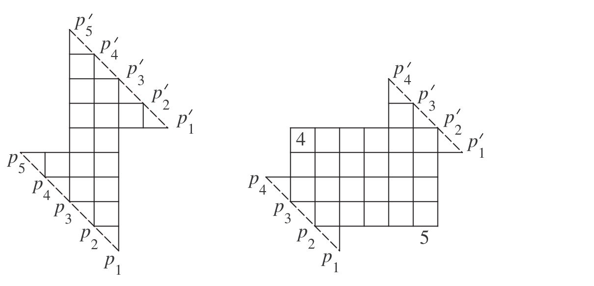
A diagram $D$ is a $5$-tuple $(k,m,r,P,Q)$, where $k$ is a positive integer, $m$ and $r$ are non-negative integers, $P$ is a lattice path from $(k-1,0)$ to $(k-1+m,r)$, and $Q$ is a lattice path from $(0,k-1)$ to $(m,k-1+r)$ that never goes below $P$. For $i$ with $1\leq i\leq k$, let $p_{i}$ be $(k-i,i-1)$ and let $p^{\prime}_{i}$ be $p_{i}+(m,r)$. Let $L$ and $L^{\prime}$ be the lines of slope $-1$ that contain the points $p_{i}$ and $p^{\prime}_{i}$, respectively. The region $R(D)$ of a diagram $D$ is the set of points in $\mathbb{R}^{2}$, including the boundary, enclosed by the paths $P$ and $Q$ and the lines $L$ and $L^{\prime}$. The edges of $D$ are the segments between lattice points in $D$ that are distance $1$ apart. Assign label $i$ to an edge in $D$ if it is the $i$-th step in some lattice path that starts at a point on $L$; thus, edges are labelled with the elements of $[m+r]$. A b-path is a lattice path contained in the region $R(D)$ that starts at a point $p_{i}$ and ends in the corresponding point $p_{i}^{\prime}$. Thus, any b-path contains $r$ North steps and $m$ East steps, and the edges are labelled, in order, $1,2,\ldots,m+r$. The label-set of a b-path $T$ is the set of labels on the North steps of $T$. Let $\mathcal{B}(D)$ be the set of all label-sets of b-paths in $D$. We now show that $\mathcal{B}(D)$ is the set of bases of a multi-path matroid, which we denote by $M[D]$. (To recover multi-path matroids in complete generality, replace the labels $1,2,\ldots,m+r$ with the elements $x,\sigma(x),\ldots,\sigma^{-1}(x)$, respectively. In much of the rest of the paper, we favor the notational simplicity gained by having $[m+r]$ be the ground set of $M[D]$.)

References

- [1] A. Björner, The homology and shellability of matroids and geometric lattices, in: Matroid Applications, N. White, ed. (Cambridge University Press, Cambridge, 1992) 226–283.
- [2] J. Bonin, A. de Mier, and M. Noy, Lattice path matroids: enumerative aspects and Tutte polynomials, J. Combin. Theory Ser. A 104 (2003) 63–94.
- [3] J. Bonin and A. de Mier, Lattice path matroids: structural aspects, arXiv:math.CO/0403337 v1 21 Mar 2004.
- [4] T. Brylawski and J. Oxley, The Tutte polynomial and its applications, in: Matroid Applications, N. White, ed. (Cambridge University Press, Cambridge, 1992) 123–225.
- [5] C. J. Colbourn, J. S. Provan, and D. Vertigan, The complexity of computing the Tutte polynomial on transversal matroids, Combinatorica 15 (1995) 1–10.
- [6] J. Edmonds and D. R. Fulkerson, Transversals and matroid partition, J. Res. Nat. Bur. Standards Sect. B 69B (1965) 147–153.
- [7] O. Giménez and M. Noy, On the complexity of computing the Tutte polynomial of bicircular matroids, Combin. Probab. Comput. to appear.
- [8] F. Jaeger, D. Vertigan, and D. J. A. Welsh, On the computational complexity of the Jones and Tutte polynomials, Math. Proc. Cambridge Philos. Soc. 108 (1990) 35–53.
- [9] J. G. Oxley, Matroid Theory, (Oxford University Press, Oxford, 1992).
- [10] D. Vertigan, Bicycle dimension and special points of the Tutte polynomial, J. Combin. Theory Ser. B 74 (1998) 378–396.
- [11] D. Vertigan and D. J. A. Welsh, The computational complexity of the Tutte plane: the bipartite case, Combin. Probab. Comput. 1 (1992) 181–187.
- [12] D. J. A. Welsh, Complexity: Knots, Colourings and Counting, (Cambridge University Press, Cambridge, 1993).