Higher connectivity of graph coloring complexesThanks: Research is partially supported by the Swiss National Science Foundation, and by the Swedish Research Council
Abstract.
The main result of this paper is a proof of the following conjecture of Babson & Kozlov:
Theorem. Let be a graph of maximal valency , then the complex is at least -connected.
Here denotes the polyhedral complex introduced by Lovász to study the topological lower bounds for chromatic numbers of graphs.
We will also prove, as a corollary to the main theorem, that the complex is -connected, for .
Key words and phrases:
Fundamental group, Hom -complexes, Kneser conjecture, Lovász conjecture, graph homomorphism, graph colorings, chromatic number, homology, valency, -connectivity2000 Mathematics Subject Classification
primary 05C15, secondary 57M151. Introduction.
Given a graph and a positive integer , there is a construction of a topological space, which can be thought of as a space of all -colorings of . This space, denoted , is a polyhedral complex, whose set of vertices coincides with the set of all allowed vertex colorings of that use at most colors.
If , then this space is empty, otherwise, it possesses a meaningful topology. Intuitively, the cells of of positive dimension encode ”homotopies of colorings”, i.e., in some sense, continuous procedures of changing one allowed coloring into another one. The general definition is given in subsection 2.2.
-complexes were introduced by Lovász, [10], to study topological lower bounds for chromatic numbers of graphs. The special case is the motivating example, since it turns out to be homotopy equivalent to the previously well-studied neighborhood complex . Recall that neighborhood complexes are the ones which were so spectacularly used by Lovász to resolve the Kneser Conjecture, see [8, 9].
Meanwhile, the other -complexes are not as well-understood. The family of complexes constitute one instance that has been studied lately, in connection with the proof by Babson & Kozlov of the Lovász Conjecture, [1, 2, 3].
It has also been recently proven by the authors, see [6], that for two arbitrary cycles and , the connected components of the complex are either points, or are homotopy equivalent to circles.
The intuition tells us that, if the maximal valency of the graph is small and the number is relatively large, then there should be a lot of freedom in completing the -colorings of locally. Expressed topologically, we may hope that the complexes will be highly connected.
To say that is -connected is the same as to say that it is nonempty. It is well-known that a sufficient condition is provided by requiring that the maximal valency of is at most (the most primitive coloring procedure works). Next, it was shown in [2, Proposition 2.4] that, if the maximal valency of is at most , then is connected (-connected).
Motivated by these special cases and by some further computational evidence, Babson & Kozlov made the conjecture which initiated our present study.
Conjecture 1.1.
[2, Conjecture 2.5].
The following inequality is valid for an arbitrary graph :
| (1.1) |
In other words: for an arbitrary graph , if , then is -connected.
The main purpose of this paper is to present a proof of this conjecture. First, we analyze the situation for . In this case, we find an explicit algorithm for deforming an arbitrary loop inside to a point, thereby verifying the triviality of the fundamental group.
Not surprisingly, it is virtually impossible to generalize these explicit homotopies to higher dimensions. Instead, we choose to use Hurewicz theorem, and calculate the nullity of the appropriate homology groups instead. Again, we give an explicit algorithmic procedure for reducing an arbitrary cycle to zero, by means of adding to it appropriately chosen boundaries.
Acknowledgments. The first author would like to thank Rade Živaljević for invaluable discussions and constant encouragement.
2. Basic notations and definitions.
2.1. Notations and terminology.
For an arbitrary natural number we introduce a shorthand notation: .
For any graph , we denote the set of its vertices by , and the set of its edges by , where . In this paper we will consider only undirected graphs, so implies that . Also, our graphs are finite and do not contain loops.
Let be a graph and . Then we denote by the graph with and . The graph we will denote by .
For a graph and , let , is the set of neighbors of . Denote the valency of by , clearly . Also denote the maximal valency of , , by .
For a graph and a natural number , let denote what we call the -color-valency gap, namely, set . With these notations, the equation (1.1) can be rewritten as:
In other words, the first possibly nontrivial homotopy group of is indexed by the -color-valency gap, .
Denote with , and the complete graph (no loops), resp. the cycle with vertices, i.e., , and , . The maximal valency of is 2, for , while the maximal valency of is .
For any two graphs and , let denote the disjoint union of these graphs.
2.2. Hom complexes: definition, examples and basic properties
A standard generalization of graph colorings is provided by the following definition.
Definition 2.1.
For two graphs and , a graph homomorphism from to is a map such that if , then .
We denote the set of all homomorphisms from to by .
Definition 2.2.
is a polyhedral complex whose cells are indexed by all functions , such that if , then for all and , .
The closure of a cell consists of all cells indexed by which satisfy the condition that , for all .
Note. We follow [1] in our notations.
The set of vertices of is . We note that cells of are direct products of simplices, and that the dimension of a cell is equal to .
One can describe a labeling of the cells in rather directly: they are indexed by all -tuples of nonempty subsets of , , where , and such that, if is an edge in , then . Also, for a cell , we will denote with its -th coordinate set (and sometimes we will refer to it as -th color list of ). With these notations, .
For any three graphs , and , the following is true:
| (2.2) |

3. The fundamental group of .
We are now ready to study the fundamental group of the graph coloring complexes.
Let , resp. , denote the cardinality of a maximal independent set in , resp. the number of vertices of . We shall write and whenever it is clear which is meant. For an arbitrary graph , label the vertices with , such that is a maximal independent set.
Lemma 3.1.
Let be an arbitrary graph, and . Assume that . For an arbitrary , any closed edge-path in the -skeleton of , such that the first coordinates of every vertex in this path are elements of the set , can be deformed by subsequent homotopies so that these coordinates will be elements of the set .
Proof.
Each vertex of the complex can be described by -tuple , where , for .
First of all, in any closed edge-path we may assume that successive vertices are distinct. Otherwise, if for some , we could delete and obtain a homotopic path. Hence, from now on, we shall implicitly replace every path with a homotopic path where no two successive vertices are equal.
We will give an algorithm which performs the deformation, the existence of which is claimed in our lemma. Formal description of steps, together with proofs of their correctness, will be given after description of the algorithm.
Let be a closed path satisfying conditions of Lemma 3.1, and let be the vertices of this path. Note that each , for , is described by a -vector and differs from in exactly one component.

The input for our algorithm is the path , and the algorithm consists of two parts. In the first part, we repeat both of the following steps for all , in increasing order.
- Step 1:
-
Inserting two new vertices between all those neighboring pairs and from the path which both have on -th position; result of step 1 is a path .
- Step 2:
-
Deleting those vertices from the path which use color on the graph vertex ; result of this step is the path .
After the first phase, we obtain a path with the property that colors used on vertices are elements of the set .
Now, input for the next stage is the path , and we repeat both steps 3 and 4 for all , again in the increasing order.
- Step 3:
-
Inserting two new vertices between those neighboring vertices of the path , and , which both have on -th position; result of step 3 is the path .
- Step 4:
-
Deleting those vertices from the path which use color on ; result of this step is the path .
Output of this algorithm is a path , and for each vertex of this path, colors used on are from the set .
Now we give detailed description of all the steps.
Step 1. If occurs in -th position for both and we will “separate” and by adding new vertices to the given path. We have
where . We have indicated only and components which are different in these two vertices. Let
where both sets are indexed with those , for which . Obviously, we have and, since , there exists , such that
are vertices of . In another words, we have a vertex of of bounded degree, and two colorings that differ in only one vertex, so we find an alternative color left for the vertex .
Deformation of the subpath into is a homotopy over the 2-cell , see Figure 3.

Let be the path obtained by the first step.
Step 2. In this step we will remove from the path those vertices which have in the -th position. In this case, as a result of the first step, we have the following situation:
where .
Deletion of is either a homotopy over the 2-cell , or, if , a homotopy over the 1-cell , see Figure 4.

Let be the path obtained after this step. It is clear that this path does not have any vertices which have in the -th position.
After the first stage of our algorithm, we obtain a path . Set , that is , where for all ( is the length of the path ). In this path, is not in -th position of any vertex, where .
Step 3. If occurs in -th position for both and we will, similar to the first step, “separate” them by adding new vertices to the given path. We start with
where . Since vertices labeled form an independent set, we know that . Hence, the color does not occur among the neighbors of in , or in . Therefore,
are legal -colorings, and hence are also vertices of . Then, the deformation of the subpath into is a homotopy over the 2-cell .
Let now be the path obtained by the third step.
Step 4. Similar to the Step 2, all the vertices from the path which have in the -th position are deleted:
where .
Deletion of is homotopy over the 2-cell (or, if , over 1-cell ).
Let be the obtained path. We can
see that after this step -th coordinate of any vertex from this
path is in the set .
Finally, we arrive at the path which has been obtained by a sequence of elementary homotopies from the original path and has the additional property that the first coordinates of every vertex from this path are elements of the set . ∎
Note. This proof was motivated by the ideas from [4].
We would like to remark, that the Steps 1 and 2 can be combined to obtain one reduction step encoding the following transformation: we find the first vertex where occurs in -th position of two vertices in a row, then we glue in a square, as in Step 1, and then we clip off a triangle, as in Step 2, see Figure 5.
The outcome of this procedure will be a shortening of the undesired part (here meaning is in the -th position) by 1. With this line of argument, one has two special cases to attend to. First, if the undesired vertices come only as singletons, then we clip them all off as in Step 2. Second, if all vertices are undesired, then gluing in an arbitrary square, as in Step 1, reduces this to the case which we considered first.
The Lemma 3.1 is the crucial step in the proof of the main result of this chapter.
Theorem 3.2.
Let be any graph. If , then is simply connected.
Proof.
We will prove that is simply connected using induction on the maximal valency of . We will use the same notations as in the previous lemma.
Suppose that the maximal valency of a graph is and that . Then is disjoint union of points and, using (2.2), we conclude:
.
is a simplex, so is contractible, and hence -connected.
Assume now that the maximal valency of is equal to and that . Let be any closed edge-path in -skeleton of . Since is a polyhedral complex, it is clear that it is sufficient to consider only these paths.
Using Lemma 3.1 iteratively, we can homotopicaly transform this path to a path which has the property that the first coordinates of any vertex from this path are equal to , where is a maximal independent set in . Hence, the original path is homotopic to a path lying inside the subcomplex . That path is contractible to a point by induction hypothesis, since is a maximal independent set, and therefore the maximal valency of is strictly less then . ∎
We will now evaluate the fundamental group of for one case when the maximal valency of a graph equals .
Proposition 3.3.
is the free product of copies of , where .
Proof.
Since is a connected graph, we can choose a spanning tree and contract it. Then we get a bouquet of circles, where is the number of vertices and number of edges of this graph. It is easy to see that and, since is -regular, . This gives us the claim of the proposition. ∎
4. Homology groups of complexes and the main theorem.
In the previous section we proved that, if the maximal valency of is , then is simply connected (or -connected), for all . Here we will prove a more general statement using the notations and ideas from Lemma 3.1 and Theorem 3.2.
First, we will introduce a new notation. Let be a graph with the set of vertices and let be an integer. Then, for all , we define a subcomplex of in the following way:
In other words, only colors have been used in the first vertices. For example, Lemma 3.1 is exactly pushing the loops from into the subcomplex . If it is clear which graph is meant, we will use the notation instead of .
Let us again label the vertices of in the same way as we did in Lemma 3.1, that is so that the vertices labeled form a maximal independent set.
Lemma 4.1.
Let be a graph with the maximal valency equal to . If is a -cycle in , where and , then there exist a -cycle in such that and represent the same element in .
Proof.
Recall that a cell from can be described by the -tuple , where for all (). Rephrasing the definition above, we get
for . The orientation of the cells can be chosen so that the boundary operator is given by
where denotes the index, for which , , and the sum is taken over all , such that .
Like in the proof of Lemma 3.1, we give a description of an algorithm whose output is a cycle , whose existence is claimed in this lemma. General scheme of the proof is the same as for already mentioned Lemma 3.1. Namely, we first get rid of color on vertices , and afterwards we are removing color from color lists on all vertices from the chosen maximal independent set, see Figure 2.
Input for our algorithm is the -cycle . For each , in the increasing order of , we repeat both of the next two inductive steps.
- Step 1:
-
This is the only step in our proof where we use the assumption about maximal valency of . In this step we eliminate all cells from the cycle such that . Result of this step is a cycle with the property that -th color list of each cell from which contains has length .
| Now we have new, iterative, step. Namely, step 2 is repeated for cycles , starting from , until there exists a cell such that . |
- Step 2:
-
Transforming the cycle to a homologous cycle with the property that, for all , if , then .
| Since length of each color list is certainly less or equal to , repetition of step 2 will stop after finite number of iterations, and we will get a cycle . |
Input for the second stage of this algorithm is the cycle . For each cell of this cycle, . Again, we repeat the following inductive steps for all , in the increasing order:
- Step 3:
-
We eliminate all cells from the cycle such that . Result of this step is a cycle with the property that -th color list of each cell from which contains has length .
| Step 2 is repeated for cycles , starting from , until there exists a cell such that . |
- Step 4:
-
Transforming the cycle to a cycle , such that and represent the same homology element, and such that, if , then , for all cells .
| By the same argument as in the first part, repetition of step 4 will stop after finite number of iterations, and we will get a cycle . In the case when , we label the resulting cycle with . |
After describing the algorithm, we give a detailed description of steps:
Step 1. Let be a -cell appearing in the chain , such that , and let have the coefficient in . The dimension of is equal to , and we have:
since the second term in the middle sum is 0, the third term in the middle sum is nonnegative, and . It follows that
as we recall that, by assumption of the lemma, . Hence, there exists such that . Obviously, . Set , where comes from the appropriate incidence number, i.e., in our notations
Clearly, represents the same homology element as . Furthermore, the number of cells appearing in , such that , is strictly less then number of such cells appearing in , since we have just eliminated the appearance of the cell . We repeat this procedure until we get cycle in which there are no cells such that .
Step 2. Suppose now that we have a cycle , , which represents the same element in homology as , and which has the additional property that , for each cell appearing in , such that . If no such cell exists, we are done with this case, and we set . Since , we will always come to this case after a finite number of steps.
Assume now there exists a cell such that , and let us construct . Assume further that , where , , , and ’s are pairwise different -cells from . Then we can write , where
If , then we set , so assume .
Clearly, . Now let , where is a subchain consisted of all cells from the boundary such that , is a chain of all cells from such that -th set has elements and contains ; finally consists of all cells where we do not have in -th coordinate set. Since and the chain cannot contain any cell , such that and , we conclude that .
Furthermore, let us fix the sets , for all . We denote by the chain of all cells from such that , for all . Obviously, all these parts must also be .
Let us also consider the corresponding subchains
| (4.3) |
in the chain , where
It is clear that must be the part of the boundary of , where the deleted element is in , and is different from .
Let us construct a new cycle , homologous to , with the property that for all cells appearing in it with and , for , we have , that is with the corresponding .
Case : Let be a cell from with coefficient , and let , for some . Since , there must exist another cell in , such that , for . Let us denote with . It is clear that . Also, the number of cells of the corresponding for the cycle , where
is reduced at least by one. Repeating this procedure, we will eventually get a chain with the corresponding equal to zero.
Case : Define a map , where is equal to
and is simplex with the vertex set , in the following way: for a cell , set
and then extend it by linearity. Function is clearly a bijection between cells and is a -chain in . Let us now prove that this chain is in fact a cycle.
For , let where . In order to avoid ”ugly” formulas we will use instead of . Then we have:
On the other hand we have
and hence,
Since a simplex is acyclic, there exists an -dimensional chain in such that
Let now . Clearly, is a -chain. We need to check that . The condition for that is , for adjacent to . This is clear for , , since then , for . Assume that there exists adjacent to , such that . By construction of , we know that . Since , for any , we arrive at a contradiction.
Let now , where
Similarly to what we have done before, one can prove that
where . Since is a bijection, we conclude that . Finally, let .
After repeating the procedure described above for all combinations of sets appearing in the decomposition of to subchains of the form (4.3), we will get a chain such that , for all cells appearing in it with nonzero coefficients, and with .
The following observation is important for our argument. If for all cells from we have that , for and , then also for all from and , we have .
After first phase, we shall eventually obtain a chain which has the following additional property: for all cells appearing in this chain with a nonzero coefficient, we have , for (the original condition of the lemma preserved), and , for .
Step 3. This step is almost the same as Step 1. Namely, assume is a cell from such that coefficient of in is , and . Then , since , for all such that . Again, , where , is a chain homologous to and number of cells from such that is strictly less then number of such cells from . We repeat this procedure until we get cycle in which there are no cells such that .
Step 4. This step is very similar to the Step 2. The only difference is that we are ”removing” (instead of ) from -th coordinate sets of each cell from the chain and obtain a new chain such that for each from . By the observation that we have made after Step 2, we see that, for all cells from and for all , we have . In the case when , we set .
Now it is easy to see that and that , is a boundary of some -chain of , and we have proved our claim. ∎
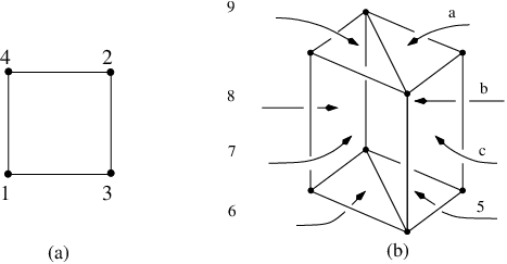
Example. Now we will illustrate the proof of Lemma 4.1 on a cycle from . For simplicity, we will use slightly different notations for cells, for example we will write instead of . We have ordered vertices of as described in Lemma 3.1, see Figure 6(a).
Let . It is easy to check that . Figure 6(b) depicts the part of the complex formed by all the cells from .
First we will eliminate from and , for all cells from our chain .
For we obviously do not have Step 1. Hence, , where , , and is the rest of . Let and . Then , , and finally,
Again, , and , since . Then , where . It is easy to see that and . If we do the same thing for the subchain , we will get the cycle .
Now we apply Step 1 for : Let , . We see that, in this case, could be any element from the set , but for convenience, we will choose . Then . Repeating this for all cells such that their fourth coordinate set is , with additional remark that we always pick , we get a chain .
Let us now remove from the first two coordinate sets of all cells from .
First we apply Step 3: Let . Then and . If we do the same thing for all other cells from , finally we get .
Theorem 4.2.
Let be an arbitrary graph, then
Note. As mentioned above, it was proved in [2] that if . Also, it is a direct corollary of Theorem 3.2 that if . Hence, we can assume that .
Proof.
Let and be the same as in Lemma 3.1 and Lemma 4.1. Also, let be a -cycle from , that is dimension of all cells from is equal to and , where the boundary operator is defined in the proof of Lemma 4.1. In order to prove that , we need to prove that bounds. Again, we will use induction on the maximal valency of .
Let the maximal valency of a graph be zero. In the Theorem 3.2 we proved that in this case is contractible and hence, for all and there exists a chain such that .
Assume now that the maximal valency of is . By Lemma 4.1, there exists a cycle which is homologous to and which has the property that, for all cells with nonzero coefficients in this cycle and for all , . Hence, is isomorphic to a cycle inside . The set is a maximal independent set in , therefore, the maximal valency of is strictly less then the maximal valency of . It follows that is a boundary in by the induction hypothesis. We conclude that there exists a -chain in , such that . ∎
Remark 4.3.
It was proved in [1] that:
, for .
This fact is a direct corollary of the previous theorem since the maximal valency of is equal to .
Finally, we are able to put the pieces together and prove the Conjecture 1.1.
Proof of the Conjecture 1.1.
Let us now deal with case . By the Theorem 3.2, is 1-connected, and by the Theorem 4.2 we have,
for all . By a standard corollary to the Hurewitz theorem (see, for example, [5, 10.10 Corollary, page 479]), we have that , for all , and, hence by definition. ∎
Remark 4.4.
We know that the result of Conjecture 1.1 is sharp for several classes of graphs, for example for odd cycles and complete graphs.
Remark 4.5.
By the same corollary we used in the proof of Conjecture 1.1, we conclude that .
Corollary 4.6.
The complex is -connected, for arbitrary integers .
References
- [1] E. Babson, D.N. Kozlov, Topological obstructions to graph colorings, Electron. Res. Announc. Amer. Math. Soc. 9 (2003), 61–68.
- [2]
E. Babson, D.N. Kozlov, Complexes of graph
homomorphisms, preprint, 20 pages, submitted in 2003.
arXiv:math.CO/0310056 - [3]
E. Babson, D.N. Kozlov, Proof of the Lovász
Conjecture, preprint, 40 pages, submitted in 2004.
arXiv:math.CO/0402395 - [4] I. Bárány, S.B. Shlosman, A. Szücs, On a topological generalization of a theorem of Tverberg, J. London Math. Soc. (2) 23 (1981), no. 1, 158–164.
- [5] G. Bredon, Topology and geometry, Corrected third printing, Graduate Texts in Mathematics, 139, Springer-Verlag, New York, 1997.
- [6]
S.Lj. Čukić, D.N. Kozlov, Complexes of graph
homomorphisms between cycles, preprint, 15 pages, submitted in 2004.
arXiv:math.CO/0408015 - [7] A. Hatcher, Algebraic Topology, Cambridge University Press, Cambridge, 2002.
- [8] M. Kneser, Aufgabe 360, Jber. Deutsch. Math.-Verein. 58 (1955).
- [9] L. Lovász, Kneser’s conjecture, chromatic number, and homotopy, J. Combin. Theory Ser. A 25, (1978), no. 3, pp. 319–324.
- [10]
L. Lovász, Topological nonexistence results in complexity theory and combinatorics,
http://research.microsoft.com/users/lovasz/ppts/topology1.ppt