Strong S-equivalence of Ordered Links
Abstract.
Recently Swatee Naik and Theodore Stanford proved that two S-equivalent knots are related by a finite sequence of doubled-delta moves on their knot diagrams. We show that classical S-equivalence is not sufficient to extend their result to ordered links. We define a new algebraic relation on Seifert matrices, called Strong S-equivalence, and prove that two oriented, ordered links and are related by a sequence of doubled-delta moves if and only if they are Strongly S-equivalent. We also show that this is equivalent to the fact that can be obtained from through a sequence of Y-clasper surgeries, where each clasper leaf has total linking number zero with .
1. Introduction
A fundamental problem in knot theory is to classify knots and links by type, and several algebraic and geometric invariants have been developed with this goal in mind. Recently Swatee Naik and Ted Stanford have shown an equivalence between S-equivalence of knots, a purely algebraic invariant, and the doubled-delta move on knot diagrams, a purely geometric relation. They prove that two knots are related by a sequence of doubled-delta moves if and only if the knots are S-equivalent [NS]. We prove that the analogous connection for links between S-equivalence and the doubled-delta move, posed as a question by Stavros Garoufalidis, is false.
We define a new invariant of ordered links called Strong S-equivalence that is in many ways better suited for links than the classical definition of S-equivalence. With this new definition, we are able to prove a theorem analogous to Naik and Stanford’s result for links. Our main theorem also ties these results to the emerging subject of clasper surgery, which has strong connections to the field of “quantum topology,” an area of study that encompasses the Jones polynomials, Vassiliev invariants, and the Kontsevitch integral.
Main Theorem.
Consider two oriented, ordered -component links and . The following four statements are equivalent:
i. can be obtained from through a sequence of doubled-delta moves.
ii. and are related by a sequence of -clasper surgeries, where each leaf of each clasper has total linking number zero with the link.
iii. and are Strongly S-equivalent.
iv. For some choice of Seifert Surfaces and and bases of , and have identical ordered Seifert Matrices.
Throughout the paper, a link with -components is a subset of , or of , that consists of disjoint, piecewise linear, simple closed curves (a link with one component is a knot). Unless otherwise noted, all links will be oriented and ordered. Seifert surfaces for links will be required to be connected, and will denote the minimal genus among possible Seifert surfaces.
2. The Doubled-Delta Move
The Delta Move
Before defining the doubled-delta move, we look first at the simpler (single) delta move. The delta move shown in Figure 1 is a particular move on knot or link diagrams. Given a link containing the tangle in Figure 1a, replace the tangle with that of Figure 1b in such a way that respects the free ends.

It is clear that the delta move preserves the pairwise linking numbers of the components, since for each pair of strands, the move changes neither the crossing nor the orientation. Though less obvious, the converse is also true, as proved by Murakami and Nakanishi in [MN]: two links have the same sets of pairwise linking numbers if and only if they are equivalent under delta moves. Since a knot is a one-component link, it follows that any two knots are equivalent under delta moves.
The Doubled-Delta Move
The doubled-delta move is similar to the single delta move, with each of the three strands being replaced by a pair of oppositely oriented strands. The link components that comprise the six affected strands are irrelevant. The doubled-delta move is more restrictive than the (single) delta move, but it still preserves the pairwise linking numbers.

Borromean Surgery
The delta move and doubled-delta move partition knots and links into equivalence classes. Two links are said to be in the same class if they are related by a sequence of such moves. However, unlike many of the basic moves that change a knot or link diagram, the delta and doubled-delta move are closely related to other operations used by topologists in a variety of contexts. In Figure 3, we see that the effect of the delta move is the same as “adding in” Borromean rings.

Another name for the operation depicted in the figure is Borromean (or Borromeo) surgery. We will see in Section 3 how Borromean surgery relates to claspers, and thus to grope cobordisms, finite-type invariants, and other ideas of low-dimensional topology.
3. Claspers
Under what conditions are two links related by a sequence of doubled-delta moves? This question is interesting to many topologists in the context of clasper surgery, a special case of which is Borromean surgery. Claspers were first defined by K. Habiro [H], where they arose in the context of finite-type invariants. Habiro demonstrated how the theory of claspers provides an alternative calculus under which one can study finite-type invariants of knots and 3-manifolds. Claspers also were implicit in the work of Goussarov [Gu1][Gu2]. Today, they are studied across various fields of low-dimensional topology. In addition to applications of finite-type invariants, P. Teichner and J. Conant examine claspers’ relationships to grope cobordisms [CT], and S. Garoufalidis uses clasper surgery [GL] to better understand the Kontsevich integral and concordance classes of knots.
Definition
A clasper is a compact surface constructed from the following three types of pieces:
- •
edges, or bands that connect the other two types of pieces
- •
nodes, or disks with three incident edges
- •
leaves, or annuli with one incident edge.
The annuli that comprise the leaves may be twisted with any number of full twists. We call this number the framing of the leaf. Figure 4a shows a clasper with zero-framed leaves.

Clasper Surgery
Assume that a clasper is embedded in a 3-manifold . To do surgery on the clasper means to remove a handlebody neighborhood of the clasper from a -manifold , and glue it back in a prescribed way according to the clasper and its framing. In particular, we associate a link to the clasper as in Figure 4b using the following substitutions: each node of the clasper is replaced by a copy of the positive, zero-framed Borromean rings, and each edge is replaced by a positive Hopf link. Leaves of the clasper do not contribute additional link components, but the framing of a leaf does determine the framing of the Hopf link component corresponding to that leaf’s adjacent edge. Clasper surgery, then, is really integer surgery on the associated framed link.
An important property of clasper surgery is that it preserves the homology of the affected manifold. When each leaf of the clasper “clasps” a knot or link and at least one leaf bounds a disk in , the result of the surgery is a new knot or link in the same -manifold.
Surgery on the simplest clasper–the strut, with a single edge and two leaves–can accomplish a single crossing change in the original knot. Since the crossing change is an unknotting relation, all knots are related by strut-clasper surgery. The simplest interesting clasper, then, is the -clasper. One may also argue that the -clasper is the most interesting clasper, since any larger clasper may be realized as several -claspers by expanding edges of the larger clasper into Hopf-linked pairs of leaves [H].
Null Claspers
In [GR], S. Garoufalidis and L. Rozansky discuss null claspers, those whose leaves are null-homologous links in for a 3-manifold and knot . Such leaves are sent to zero under the map ; in other words, each leaf has algebraic linking number zero with the knot. Garoufalidis and Rozansky explain that null claspers have been used to demonstrate a rational version of the Kontsevich integral and can be used to define a notion of finite-type invariants. In Lemma 1.3 of [GR], they show that surgery on null claspers preserves not only the homology of a knot complement, but also the Alexander module and Blanchfield linking form. Furthermore, null clasper surgery describes a move on the set of knots in integral homology spheres that directly corresponds to the doubled-delta move.
Extending Garoufalidis’s and Rozansky’s definition to links, for the pair , where is a 3-manifold and is a link, a null clasper would be one whose leaves have linking number zero with each component. Unfortunately, the doubled-delta move acts on the strands of a link independently of the link components. Therefore, in considering the relationship between claspers and the doubled-delta move, our interest is with a slightly larger class of claspers: those in which each leaf clasps several strands of the link in such a way that the total linking number with all link components is zero.
We claim that when the leaves of a zero-framed -clasper each have total linking number zero with the link, the -clasper surgery has the same effect on the link as a finite sequence of doubled-delta moves, as well as that of Borromean surgery. This is one of the implications of our main theorem, and is illustrated in Figure 10.
4. S-equivalence and the Doubled-Delta Move
The Seifert Matrix
Many of the basic algebraic invariants of knot theory, including the Alexander module, the Conway polynomial, and the signature, depend only on the Seifert matrix of a knot or link, which is readily computable but not uniquely defined.
For every -component link in , there is a Seifert surface associated to the link, where is a connected, oriented, embedded surface with the components of as its boundary. Given a basis of , we can associate a Seifert matrix to the link , where the entries of are defined from the linking number of two basis elements. In particular, , where is a pushoff of in the positive normal direction.
Classical S-equivalence
S-equivalence is a notion that has been widely considered for both knots and links [Go] [K] [Li]. Two square integral matrices and are said to be S-equivalent if can be transformed into by a finite sequence of integral congruences (that is, for some integral matrix with ) and row or column enlargements/reductions of the form
A more precise statement of these definitions is given in section 5. Up to S-equivalence, Seifert matrices are well-defined for knots and links.
Relationship to the Doubled-Delta Move
Despite being a purely algebraic relation, S-equivalence has geometric implications for knots. In particular, S. Naik and T. Stanford prove that two knots are S-equivalent if and only if they are equivalent by a sequence of doubled-delta moves [NS].
One might assume that a similar statement should be true of links. Is the S-equivalence of two links enough to guarantee that they are equivalent under a sequence of doubled-delta moves? This question was posed by Stavros Garoufalidis in the context of clasper surgery, and given that all the definitions leading up to S-equivalence are the same for links as they are for knots, it seems that the analogous proof for links should follow in a straightforward fashion from the proof of Naik-Stanford. The question seems plausible, but in fact it is false. We prove by counterexample in Proposition 4.1 that two S-equivalent links are not necessarily related by a sequence of doubled-delta moves.
Proposition 4.1.
S-equivalence is not a sufficient condition for two links to be related by a sequence of doubled-delta moves.
Proof.
The two links and depicted in figure 5 are S-equivalent but not related by a sequence of doubled delta moves.

Note that the pairwise linking numbers of the first link are while for the second link they are . Since the doubled-delta move preserves pairwise linking numbers, these two links cannot be related by doubled-delta moves.
The fact that the two links are S-equivalent can be seen by choosing Seifert Surfaces as in figure 6,

with bases and . Each of the surfaces can be viewed as a punctured 2-sphere with a Y-shaped band glued along the boundary, where each of the three strips of the Y is twisted according to the desired linking numbers. The Seifert matrices are then and , respectively. The matrix satisfies the condition , demonstrating that the two links are in fact S-equivalent. ∎
Finding the sufficient conditions to extend the Naik-Stanford theorem will require some new definitions, treated in section 5.
5. Strong S-equivalence
As shown in Proposition 4.1, the classical definition of S-equivalence is inadequate for the proof of our main theorem, and actually it seems inappropriate for links in many contexts. Treating a link as a disjoint knot, S-equivalence regards the entire link as a whole, without reference to the individual components. Strong S-equivalence, defined below, better respects the boundary components of a Seifert surface, and hence the components of the link.
Let be an oriented, ordered link in . Let be a Seifert surface for with boundary components, and let denote the genus of . That is, is an oriented surface with . Construct an ordered basis for , where is represented by the th component of . Define the Seifert pairing , where is a pushoff of in the positive normal direction. We introduce the following term:
Definition.
A matrix representing with respect to an ordered basis of the form above is called an Ordered Seifert Matrix for the oriented ordered link .
Remark 5.1.
has the form of a block matrix , where is an block and is a block. The block is completely determined by the pairwise linking numbers of , and has the following properties:
for , and
if and .
The first of these properties is somewhat less obvious. If we let be the homology class represented by , then the class , since it is represented by the boundary of . Then
The following two definitions can be found in [K], as they are essential to the classical definition of S-equivalence.
Definition.
We say two integral square matrices and are congruent if for some integral matrix with .
Definition.
For integral square matrices and , we say that is an enlargement of , or is a reduction of if
With a slight modification of these two definitions, we introduce:
Definition.
Two matrices and are Strongly S-equivalent if is equivalent to under a finite sequence of
- •
Congruences that fix the upper-left block of the matrix. That is, there exists an integral matrix , so that and , where is the identity matrix.
- •
Enlargements and reductions where the first elements of the vectors and are equal, and where the reduced matrix is for .
Note that reductions should not be allowed to reduce the size of the matrix smaller than , for in the case of Seifert matrices, this would effectively eliminate link components.
Also note that the first elements of the vectors and are equal because these entries should be zero in the intersection form of the enlarged matrix , since boundary components will not intersect any other basis elements.
Definition.
We say that two links and are Strongly S-equivalent if, for some choice of Seifert surfaces and ordered bases, and have ordered Seifert matrices and that are Strongly S-equivalent .
One might object that Strong S-equivalence imposes the “restriction” that and agree on their upper-left blocks. However, since homeomorphisms of from the pure mapping class group preserve the boundary components pointwise, any change of basis of must fix the basis elements. With Strong S-equivalence, we’re not “restricting” our definition so much as respecting the boundary components of a link.
Disk-Band Form of the Seifert Surface
It will often be useful to look at the Seifert surface in disk-band form. Any Seifert surface for a link is homeomorphic to a disk with bands attached; more importantly, we can always isotope our surface to one in disk-band form as in Figure 7, with bands interlaced in pairs and non-interlaced bands.

Within the dotted box, the bands of our surface form a string link, i.e. they may be knotted, twisted, or intertwined as long as the bands entering the top of the box match up with those that leave the bottom of the box. With the surface in this form, there is an natural choice for a basis of , with one basis element running through each of the bands. The first non-interlacing bands yield basis elements that are pushoffs of the respective boundary components and have no intersection with any other basis elements. The interlaced bands yield basis elements with the properties of a symplectic basis, i.e. one whose intersection form is the block sum . We coin the term semi-symplectic to refer to this natural choice of basis. A semi-symplectic basis is an ordered basis, but the converse is not necessarily true.
Properties of Strong S-equivalence
Proposition 5.2.
Pairwise linking number is an invariant of Strong S-equivalence.
Proof.
If two links and are Strongly S-equivalent then, regardless of the choice of ordered Seifert matrices and , the upper left blocks of and will necessarily agree. That is, for , ,
Furthermore, by property of Remark 5.1,
Thus all the pairwise linking numbers for agree with those for . ∎
Proposition 5.3.
Any two ordered Seifert matrices for an oriented ordered link are Strongly S-equivalent.
Proof.
Let and be two ordered Seifert matrices for with respect to Seifert surfaces and and bases and .
By Lemma 5.2.4 of [K], any two connected Seifert surfaces and of a link are ambient isotopic after modifying them by a finite sequence of 1-handle enlargements. In other words, there are two ambient isotopic surfaces and such that is the result of several 1-handle enlargements of . Without loss of generality, we can consider just the following case: suppose some surface is ambient isotopic to , a single 1-handle enlargement of . Let be a meridian (technically, the belt sphere) of the 1-handle and choose a closed curve that intersects the meridinal disk (technically, the co-core) exactly once. Then one of
is a Seifert matrix for with respect to the basis for . The matrix on the left, , corresponds to a 1-handle attached so that its core lies on the negative side of the surface, while corresponds to a 1-handle with its core on the positive side of the surface. We will treat only the case and note that the case follows similarly. The zeros in the last column of come from the fact that a positive pushoff of the meridian, , will not link any of the basis elements except . The last row of is all zero because a negative pushoff of the meridian will not link any of the basis elements. Since for any Seifert matrix , is an intersection form, the first entries of the vectors and must be equal. Otherwise would be intersecting a boundary component, which is impossible. The rest of the entries of and are freely determined by the particular embedding of the new 1-handle and the choice of curve , as always with . The entry is, of course, . Note that with more restrictions on the choice of , the allowable entries of , , and could be given more structure.
By the definitions of enlargement and reduction, and are Strongly S-equivalent. This process can be iterated for any finite number of 1-handle enlargements so that the final matrix is Strongly S-equivalent to , and similarly, can be shown to be Strongly S-equivalent to , the similarly constructed Seifert matrix for .
Since is ambient isotopic to , and differ only by a choice of bases. Furthermore, since the upper left blocks of both and are determined by the link and are equal (note that has the same upper-left block as ), and are related by a change of basis that preserves the first basis elements, and they are thus Strongly S-equivalent. By transitivity, is Strongly S-equivalent to . ∎
Like its classical S-equivalence analogue, the converse of Proposition 5.3 is not true. If is a Seifert matrix for the link with respect to Seifert surface , and is Strongly S-equivalent to , is not necessarily a Seifert matrix for . The difficulty arises when is a reduction of , since it may not be possible to find a corresponding 1-handle reduction of the Seifert surface . The converse is true, however, in the special cases of congruences and enlargements. Matrix congruence corresponds to change of basis for widecheck. In order to explicitly understand how any given matrix enlargement corresponds to a 1-handle enlargement of a Seifert surface, we prove the following proposition:
Proposition 5.4.
If is an ordered Seifert matrix for the link with respect to Seifert surface , and is an enlargement of , then is an ordered Seifert matrix for with respect to a 1-handle enlargement of
Proof.
Let be a Seifert surface for with basis of that induces the Seifert matrix . We will construct the 1-handle enlargement of that has as its Seifert matrix, where either
As in Proposition 5.3, the matrix on the left corresponds to attaching the 1-handle so that its core lies on the negative side of the surface, while the matrix on the right corresponds to a 1-handle with its core on the positive side of the surface.
Let be a set of representative curves for the basis . Find two small disks in that are disjoint from the curves . These disks will be the attaching region for the 1-handle. Designate two points, and , one point on the boundary of each disk. The enlarged matrix determines the Seifert form–that is, a combination of linking and intersection numbers–of two new basis elements and with curves . The 1-handle we construct will have as a meridian and running parallel to the core. First let us construct , breaking it into two parts, and , as in figure 8. In order to be consistent with the Seifert matrix , we need to to intersect and link the curves according to the entries of the vectors and . We can extract the intersection information from the intersection form , or in particular, from the vector entries [R]. Running through the surface , will be constructed to take care of any intersections, while the handle itself, and hence , will be free to link the basis elements. Together, will then satisfy each of the entries and .

To find , the half of that will travel from to along the surface , let us look at the intersection form . The individual entries of determine how should intersect the curves ; since does not intersect at all, . The first entries of are zero, which is consistent with the fact that cannot cross a boundary component. For the last curves , choose so that . This is possible. As described previously, the basis is in correspondence with a semi-symplectic basis. For ease of construction, choose a set of curves in to be representatives of this semi-symplectic basis with the same (semi-symplectic) algebraic intersection properties. If, for any set of integers , we can construct a curve that has algebraic intersection number with each , then the same can be done for the set of curves via this correspondence. Start with a curve from to that does not intersect any of the curves . For each desired intersection with a particular curve , take (For each intersection with , take .) Continue this until all intersections are achieved, and call the final curve . Figure 9, below, demonstrates how a path from to can be chosen to intersect exactly one time and intersect exactly times.

After the intersection properties are established between and the , we shift our focus to the linking properties. As with the intersections, the linking numbers of with the are in correspondence with those of with the , so we will focus our construction on the semi-symplectic basis . The core of the 1-handle can be chosen in the complement of so that it links each of the curves the desired number of times. This is easy to see in the disk-band representation of . The core can then be fattened up to a solid handle, the surface of which is the 1-handle enlargement of We choose a curve on the surface of the handle parallel to the core, and let be one of our new basis elements. Figure 9 demonstrates how the core can be chosen to link one time and link negative one time.
Lastly, we must adjust the path along the 1-handle so that . The remedy is simple: each repeated positive or negative full twist to the 1-handle will increase or decrease by one without affecting any of the other basis elements. Figure 9 illustrates chosen so that
We have explicitly constructed a new Seifert surface for and a new basis for such that is an ordered Seifert matrix for with respect to them. ∎
6. Proof of the Main Theorem
Theorem 6.1.
Consider two oriented, ordered -component links and . The following four statements are equivalent:
i. can be obtained from through a sequence of doubled-delta moves.
ii. and are related by a sequence of -clasper surgeries, where each clasper has total linking number zero with the link.
iii. and are Strongly S-equivalent.
iv. For some choice of Seifert Surfaces and and bases of and have the same ordered Seifert Matrix.
The proofs of each implication are treated individually below:
Proof of
Proof.
Doubled-delta moves correspond to “Borromean surgery,” which is exactly the effect of -clasper surgery, where each leaf clasps pairs of oppositely oriented strands. This is depicted in figure 10.

In this figure, the relationship introduces the desired -clasper, transforms the clasper into its associated link, depicts the effect of surgery via handle slide moves, is merely the second Reidemeister move, and is the doubled-delta move. ∎
Proof of
We actually prove a stronger implication than claimed in the theorem, namely that the clasper surgery described in does not alter the ordered Seifert matrix.
Proof.
Consider a neighborhood of the clasp, as in Figure 11a. There are strands passing through the leaf, with in each direction. We can assume the strands’ directions alternate within this neighborhood. If they do not alternate, we can permute the strands by introducing inverse braids just above and below the braid in question.

Temporarily cut the strands at the neighborhood’s boundary and fill in the alternating arcs to get bands as in Figure 11b. Outside the neighborhood, apply Seifert’s algorithm to the resulting link. Then reattach the new bands at the neighborhood’s boundary to obtain a Seifert surface for the original link where the leaf of the clasper grabs bands of the Seifert surface.
Now clasper surgery is equivalent to tying these bands into Borromean rings, which doesn’t affect the linking of the bands or strands. If a basis element of runs through a band, its pairwise linking with the other basis elements is unchanged; if not, it is completely unaffected by the surgery. Thus the clasper surgery leaves the Seifert matrix unchanged. ∎
Proof of
With almost no alteration, the proof of can also be used to show that two classically S-equivalent knots or links have a Seifert matrix in common.
Proof.
If and are Strongly S-equivalent then, by definition, there are Seifert matrices and respectively such that is equivalent to under a finite sequence of enlargements , reductions , and congruences . For example, we can write a sequence of the form
| () |
In order to prove that and have a Seifert matrix in common, it will be helpful to rewrite the sequence ( ∗ ‣ 6) so that all the enlargements precede all the reductions, as in
| () |
The following lemmas establish that such an ordered sequence ( ∗ ∗ ‣ 6) exists for every pair of strongly S-equivalent matrices and show how the ordered sequence completes the proof of ..
Lemma 6.2.
.
Before proving this lemma, we first note that the simpler implication is not true. In the right-hand side, a reduction immediately follows an enlargement, so the two actions cancel each other and which is not necessarily true in the left-hand side.
Proof.
Assume that
Then let
If is a matrix, then let be the result of a change of basis that permutes the th basis element with the nd, and the st basis element with the rd. Then
which reduces to . ∎
Lemma 6.3.
.
Proof. If , and
be an enlargement of . Now let . Then
Lemma 6.4.
Any sequence of relations between Strongly S-equivalent matrices can be rewritten so that all enlargements come before all reductions, as in the sequence ( ∗ ∗ ‣ 6).
Proof.
The proof of Lemma 6.4 follows from an induction argument using Lemmas 6.2 and 6.3. For simplicity, we will use strings of the symbols {} to denote enlargements, reductions, and congruences, respectively, while omitting explicit reference to the matrices.
- •
Base Case: (Lemma 6.2).
- •
Inductive Step: Find the first enlargement that is preceded by a reduction. Note that the sequence preceding this enlargement is arranged as desired. There are two cases:
- (1)
- (2)
If this enlargement is immediately preceded by a reduction, then by Lemma 6.2, can be replaced with .
Continue the two steps above until the enlargement is immediately preceded by another enlargement.
We have reduced the number of out-of-order {} by one without increasing the number of enlargements or reductions. Continue the inductive step until there is no enlargement preceded by a reduction. ∎
We can now finish the proof of . If and are Strongly S-equivalent, then by Lemma 6.4 we may assume there exists a sequence of relations between and where all enlargements precede all reductions. Note that:
- •
If is an ordered Seifert matrix for the link with respect to Seifert surface and basis , and if , then is also an ordered Seifert matrix for with respect to a 1-handle enlargement of and the corresponding new basis . This follows from Proposition 5.4.
- •
If is an ordered Seifert matrix for the link , and , then is also an ordered Seifert matrix for , with respect to the same Seifert surface and a new basis as prescribed by the congruence.
Using the two facts above, we can “work inwards” from both ends of the ordered sequence to show that and have a common Seifert matrix (though not necessarily or ) for some Seifert surfaces and bases. Starting with and working from left to right, each enlargement or congruence yields a new Seifert matrix for . This terminates when we reach the first reduction. Similarly, since , starting with and working from right to left, each reduction or congruence yields a new Seifert matrix for . In the ordered sequence labelled ( ∗ ∗ ‣ 6) above, is a common Seifert matrix for and , as is . ∎
Proof of
The following proposition contains the bulk of content of the Main Theorem. This is the primary step that distinguishes the proof of from Naik-Stanford’s proof and uses the extra hypotheses of Strong S-equivalence:
Proposition 6.5.
If two -component links and have the same ordered Seifert matrix with respect to Seifert surfaces and and ordered bases and of and , respectively, then it is possible to arrange and into disk-band form and to find new semi-symplectic bases and for and that give rise to a new shared ordered Seifert matrix for both and .
Proof of Proposition.
We start with surfaces and and bases and of and , respectively. In transforming and into disk-band form, it is important that we keep track of the new semi-symplectic bases and in terms and . This means understanding the homeomorphisms involved in the transformation.
Both and have boundary components, and since they share an ordered Seifert matrix, both have the same genus, say . Let be an abstract surface of genus with boundary components, specifically realized as a disk with bands as in Figure 12 (i.e. the string link from Figure 7 is trivial),

where the form an ordered basis for . The intersection form for is represented by the block matrix , where .
Choose orientation-preserving homeomorphisms from the pure mapping class group, i.e. the boundary components are fixed, pointwise. Assume that the boundary component of that is parallel to is sent by to the th component of . Then
is also a basis for . So there exist invertible matrices such that denote the ordered Seifert matrices of with respect to the new bases . These homeomorphisms describe an explicit way to put and into disk band form as in Figure 7, where the two surfaces differ only by string links , of bands of the Seifert surfaces. The new ordered Seifert matrices and correspond to these “new” surfaces, but . In the construction process we lost the critical hypothesis that the ordered Seifert matrices for and were equal. We need to show that is also an ordered Seifert matrix for , with respect to a different basis.
By definition, if we have a Seifert matrix determined by a given basis, then is the intersection form for that same basis. Since homeomorphisms of surfaces preserve the intersection properties of their basis elements, will have the same intersection properties as , and thus we have that . Using this fact, we construct a matrix that we show stabilizes , in that . First we show that :
Then,
Now the key step is to find a homeomorphism of the pure mapping class group that induces with respect to the ordered basis . This, in turn, will prove that is an ordered Seifert matrix for . (Actually the pure mapping class group, which fixes the boundary components pointwise, is stronger than necessary. Fixing the boundary component-wise would be sufficient; however, the ordinary mapping class group only fixes the boundary set-wise.) For the case of knots, this key step is easy. There is symplectic, and thus is well-known to be induced by such a homeomorphism, since the map from the pure mapping class group to the symplectic group is surjective [MKS, pp. 178, 355-6]. For links however, is not symplectic, and it takes several steps to find a homeomorphism inducing .
Lemma 6.6.
The matrix is of the form where is a symplectic matrix.
Proof.
By construction, . We know by definition that and are of the form .
First we want to show that is also of the form . Let . Suppose is an inverse for . Then
so and . Thus must be of the form .
From this it is easy to see that
is also of the form .
Now we need to demonstrate that the lower right block of is symplectic. For this, we let . Then
Recall that . Since , is a symplectic matrix. ∎
Lemma 6.7.
The matrix , relative to any fixed semi-symplectic basis, is induced by a homeomorphism of the pure mapping class group.
Proof.
We want to consider to represent an action on . If were a once-punctured surface (in other words, if our link were a knot), then would be symplectic and this action would then be induced by a homeomorphism from the pure mapping class group [MKS].
Our Seifert surface is an -punctured surface. Choose a representative curve for each of the last basis elements of , where , such that the geometric intersections among representatives respect the algebraic intersections determined by the ordered Seifert matrix.
Temporarily cap off the boundary components with disks , forming a new closed surface . Consider a larger disk that encompasses all the smaller disks , but does not intersect any of . This is possible. Since the basis elements are semi-symplectic, we can cut along these curves to obtain an -punctured -gon. The disk can be chosen in the interior of this -gon such that it will encompass all of the disks (a pushoff of the -gon’s boundary will suffice).
Now , a subset of , is a once-punctured surface with symplectic basis . Where represents an action on , represents an action on and corresponds to a homeomorphism of the pure mapping class group by the surjective map mentioned above.
We can extend to , which agrees with on and fixes the remaining . We now have that the homeomorphism induces the action on . ∎
Lemma 6.8.
There is a matrix such that , and can be taken to be a product of elementary matrices where each is induced by a homeomorphism of the pure mapping class group.
Proof.
Observe that , or . Let . Right-multiplication by this matrix can be achieved by a product of several elementary matrices , which we will proceed to define.
Note that is an block. To better illustrate the construction of the , we first let be the matrix that has the entry of in the th spot and zeros elsewhere. One can verify that . Define an elementary matrix to be the identity matrix with in the spot, where , and . For example, if and then
It should also be noted that for any integer ,
Then , where .
To show that these elementary matrices are induced by homeomorphisms of the pure mapping class group, note that each fixes the first basis elements and sends to . An example of this is shown below for where and :
We need to find a homeomorphism that induces , that is, one that exactly takes to for (and ), while fixing all the other basis elements. These homeomorphisms can be realized as simple Dehn twists, and are illustrated in figure 13.

In each of these figures, the surface is represented schematically as a genus surface with boundary components. Pairs of the standard symplectic basis elements are labelled , while the boundary basis elements are labelled The notation is used to represent the effect on the curve of performing a Dehn twist about the curve . Using this notation, we show that can be taken to by the composition of Dehn twists . Similarly, .
Since each fixes the first basis elements, is induced by a homeomorphism that fixes the first boundary components of and hence fixes all boundary components. All that is required for the sake of is that the boundary be fixed, component-wise. However, as the are constructed from these simple Dehn twists, they can easily be taken to fix the boundary components point-wise. Now, , as a product of elementary matrices , is induced by the corresponding composition of the . That is, the action of on is induced by the composition of homeomorphisms . ∎
Together, Lemmas 6.7 and 6.8 imply that is induced by a homeomorphism of the pure mapping class group. Now we can use the homeomorphisms and to put and into disk and band form as in Figure 14. The basis elements are the columns of the matrix . Where was the Seifert matrix for with respect to the basis , now is the Seifert matrix for with respect to the basis . Thus the Seifert surfaces and , together with the semi-symplectic bases and , respectively, give rise to a shared ordered Seifert matrix for and . ∎
Finally, the tools are in place to prove the final implication of the Main Theorem.
Proof of .
Suppose and have the same ordered Seifert matrix with respect to Seifert surfaces and and ordered bases and of and , respectively. Proposition 6.5 states that the Seifert surfaces and can be arranged in disk-band form as in Figure 14, with new semi-symplectic bases and that each give rise to a shared ordered Seifert matrix for and .
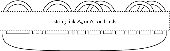
In their new disk-band form, the Seifert surfaces and differ only by the string links and of bands. Because and were chosen to be semi-symplectic, the new basis elements run straight through each band. The sets of pairwise linking numbers for and are equal, both being determined by the matrix . By Murakami-Nakanishi’s theorem [MN], and are related by a sequence of (single) delta moves. Therefore our original links and are related by a sequence of doubled-delta moves, having two oppositely oriented strands for each band of or .
Although the issue of framing on the bands of and has not yet been addressed, it is clear that the delta move doesn’t change the framing on any strand of a string link, and the doubled-delta move doesn’t alter the self-linking of any of the bands. Moreover, the framing of each band corresponds to the self-linking of the basis element running through that band and is thus the same for as for , both being determined by the diagonal entries of . ∎
References
- [CT] James Conant and Peter Teichner. Grope Cobordism of Classical Knots. Topology 43 (2004), no. 1, 119–156.
- [Ga] Stavros Garoufalidis. Links with Trivial Alexander Module and Nontrivial Milnor Invariants. preprint, math.GT/0206196.
- [GL] Stavros Garoufalidis and Jerome Levine. Concordance and 1-loop clovers. Algebr. Geom. Topol. 1 (2001), 687–697.
- [GR] Stavros Garoufalidis and Lev Rozansky. The Loop Expansion of the Kontsevich Integral, the Null Move and S-equivalence. preprint, math.GT/0003187.
- [Go] Cameron McA. Gordon. Some Aspects of Classical Knot Theory. Lecture Notes in Math., 685, Springer, Berlin, 1978.
- [Gu1] Mikhail Goussarov. Finite Type Invariants and -equivalence of -manifolds. C. R. Acad. Sci. Paris Sér. I Math. 329 (1999), no. 6, 517–522.
- [Gu2] Mikhail Goussarov. Variations of Knotted Graphs. The Geometric Technique of -equivalence. (Russian) Algebra i Analiz 12 (2000), no. 4, 79–125; translation in St. Petersburg Math. J. 12 (2001), no. 4, 569–604.
- [H] Kazuo Habiro. Claspers and Finite Type Invariants of Links. Geom. Topol. 4 (2000), 1–83.
- [K] Akio Kawauchi. A Survey of Knot Theory. Birkhäuser Verlag, Basel, 1996.
- [Le] Jerome Levine. The Conway Polynomial of an Algebraically Split Link. KNOTS ’96 (Tokyo), 23–29, World Sci. Publishing, River Edge, NJ, 1997.
- [Li] W. B. Raymond Lickorish. An Introduction to Knot Theory. Graduate Texts in Mathematics, 175. Springer-Verlag, New York, 1997.
- [MKS] Wilhelm Magnus, Abraham Karrass, and Donald Solitar. Combinatorial Group Theory. Presentations of groups in terms of generators and relations. Second revised edition. Dover Publications, Inc., New York, 1976.
- [MN] Hitoshi Murakami and Yasutaka Nakanishi. On a Certain Move Generating Link-Homology. Math. Ann. 284 (1989), no. 1, 75–89.
- [NS] Swatee Naik and Theodore Stanford. A Move on Diagrams that Generates S-equivalence of Knots. J. Knot Theory Ramifications, Vol. 12, No. 5 (2003) 717-724.
- [R] Dale Rolfsen. Knots and Links. Publish or Perish, Inc., Houston, TX, 1990.