Detecting the Growth of Free Group Automorphisms by their Action on the Homology of Subgroups of Finite Index

Adam Piggott Address: Mathematical Institute, University of Oxford, 24-29 St Giles, Oxford, OX1 3LB, UK Email address: piggott@maths.ox.ac.uk

Date: 28 July, 2004

Abstract.

In this paper we prove that if $F$ is a finitely generated free group and $\phi\in\rm{Aut}(F)$ is a polynomially growing automorphism then there exists a characteristic subgroup $S\leq F$ of finite index such that the automorphism of $S^{\rm\rm{ab}}$ induced by $\phi$ grows polynomially of the same degree as $\phi$ . The proof is geometric in nature and makes use of Improved Relative Train Track representatives of free group automorphisms.

The study of automorphisms of non-abelian free groups has been reinvigorated in recent years by a program to understand free group automorphisms as homotopy equivalences of finite graphs, called topological representatives (see, for example, [5, 3, 2, 1]). This programme is driven largely by analogy with the study of surface automorphisms and has led to significant progress in the field. In a series of papers, Bestvina, Feighn and Handel have developed powerful normal forms for topological representatives, called Improved Relative Train Track (IRTT) representatives (in analogy with train track representatives of surface automorphisms) [3, 2, 1]. This technology has allowed them to prove a number of important results, most notably the Scott Conjecture [3] and the Tits Alternative for $\rm{Out}(F)$ [2, 1]. In many applications, such as our Main Theorem, the detailed structure inherent in IRTT representatives allows one to use geometric intuition to evade difficult and unsightly cancellation arguments.

Let $F$ be a finitely generated non-abelian free group and $\phi\in\rm{Aut}(F)$ an automorphism. The growth function $\mathcal{G}_{\phi}:\mathbb{N}\to\mathbb{N}$ of $\phi$ quantifies the rate at which repeated application of the automorphism changes the ‘size’ of a basis of $F$ (see $\lx@sectionsign$ 1). The asymptotic behaviour of $\mathcal{G}_{\phi}$ does not depend on the choice of basis for $F$ and is robust when passing to subgroups of finite index. We write $F^{\rm{ab}}$ for the abelianisation of $F$ ; $\phi^{\rm{ab}}$ for the image of $\phi$ under the natural map $\rm{Aut}(F)\to\rm{Aut}(F^{\rm{ab}})$ ; $\mathcal{G}^{\rm{ab}}_{\phi}$ for the growth function of $\phi^{\rm{ab}}$ ; $\simeq$ for an equivalence relation on maps $\mathbb{N}\to\mathbb{N}$ which respects asymptotic behaviour (see $\lx@sectionsign$ 1); $p_{\rm{exp}}$ for the $\simeq$ -equivalence class containing $k\mapsto 2^{k}$ ; $p_{d}$ for the $\simeq$ -equivalence class containing $k\mapsto k^{d}$ , for $d\in\mathbb{N}$ ; and ${\rm PG}(F)$ for the subset of $\rm{Aut}(F)$ consisting of all non-exponentially growing automorphisms.

Theorem 0.1 (Main Theorem).

Let $F$ be a finitely generated free group and $\phi\in{\rm PG}(F)$ an automorphism with polynomial growth. There exists a characteristic subgroup $S\leq F$ of finite index such that, for $\theta:=\phi|_{S}$ ,

\mathcal{G}^{\rm{ab}}_{\theta}\simeq\mathcal{G}_{\theta}\simeq\mathcal{G}_{\phi}.

In the following remarks we offer some context in which to consider the Main Theorem: automorphisms of free abelian groups may, of course, be understood as elements of ${\rm SL}(n,\mathbb{Z})$ . The following theorem follows from the Jordan Canonical Form Theorem for ${\rm GL}(n,\mathbb{R})$ .

Theorem 0.2 (Traditional).

Let $F^{\rm{ab}}$ be a finitely generated free abelian group of rank $n\geq 1$ and $\phi^{\rm{ab}}\in\rm{Aut}(F^{\rm{ab}})$ an automorphism. Either $\mathcal{G}^{\rm{ab}}_{\phi}\in p_{\rm{exp}}$ or there exists an integer $\eta$ such that $1\leq\eta<n$ and $\mathcal{G}^{\rm{ab}}_{\phi}\in p_{\eta}$ .

In $\lx@sectionsign$ 3.3 below we prove, as a corollary to the IRTT Theorem, that an analogous statement may be made about the automorphisms of finitely generated (non-abelian) free groups.

Theorem 0.3 (Bestvina, Feighn, Handel).

Let $F$ be a finitely generated free group of rank $n\geq 2$ and $\phi\in\rm{Aut}(F)$ an automorphism. Either $\mathcal{G}_{\phi}\in p_{\rm{exp}}$ or there exists an integer $\eta$ such that $1\leq\eta<n$ and $\mathcal{G}_{\phi}\in p_{\eta}$ .

The Main Theorem elucidates the equality of the growth spectra of ${\rm PG}(F)$ and ${\rm PG}(F^{\rm{ab}})$ . It may also be considered an extension of the following theorem of Grossmann [6]: for each automorphism $\phi\in\rm{Aut}(F)$ there exists a characteristic subgroup $S\leq F$ of finite index such that $(\phi|_{S})^{\rm{ab}}$ is non-trivial. Further, the Main Theorem shares a theme with Lubotzky’s [8] characterisation of the inner automorphisms of $F$ as those which act trivially on the set of normal subgroups of $F$ of prime-power index.

Our proof of the Main Theorem is inspired by the following simple observations: Let $f:G\to G$ be a topological representative of an automorphism $\phi\in\rm{Aut}(F)$ . Each element $w\in F$ corresponds to a closed path $\rho$ in $G$ . The length of $w^{\rm{ab}}$ (the element of $F^{\rm{ab}}$ induced by $w$ ) in the word-metric (with respect to some generating set $A$ ) is less than the length of $w$ if and only if a generator and its inverse both appear in the unique reduced word in $A^{\pm}$ equal to $w$ . In the topological representative this corresponds to some subpath $\mu$ of $\rho$ being traversed first in one direction and later in the reverse direction as $\rho$ is traversed. We call this ‘winding’ and ‘unwinding’ $\mu$ . A key observation is that for any path $\rho$ we may construct a finite cover of $G$ such that the winding and unwinding in $\rho$ lift to different sheets of the cover. Now, $\mathcal{G}^{\rm{ab}}_{\phi}\not\simeq\mathcal{G}_{\phi}$ only if for each fastest growing closed path $\rho$ in $G$ the $f$ -iterates of $\rho$ contain significant amounts of winding and unwinding. Our strategy for proving the Main Theorem is to construct a covering graph $\tilde{G}$ of $G$ such that, for some fastest growing closed path $\rho$ , large amounts of this winding and unwinding lift to different sheets of $\tilde{G}$ .

Incidental to the proof of the Main Theorem, we prove the following corollary to the IRTT Theorem (see $\lx@sectionsign$ 3.4), the analogue of which is unknown to the Author in the case of an arbitrary finitely generated group. We also indicate how this result may be considered a corollary to the Main Theorem.

Theorem 0.4.

Let $F$ be a finitely generated free group and $\phi\in\rm{Aut}(F)$ an automorphism. Then $\mathcal{G}_{\phi}\simeq\mathcal{G}_{\phi^{-1}}$ .

Remark 0.5 (Algorithmic properties of the Main Theorem).

It is shown in [3] that there exists an algorithm to determine whether or not an automorphism $\phi\in\rm{Aut}(F)$ is polynomially growing. Given $\phi\in{\rm PG}(F)$ and an IRTT representative $f:G\to G$ of some iterate of $\phi$ , our proof of the Main Theorem shows how to construct a characteristic subgroup $S\leq F$ of finite index with the property that $\mathcal{G}^{\rm{ab}}_{\phi|_{S}}\simeq\mathcal{G}_{\phi}$ . Alternatively, without necessarily knowing an IRTT representative of an iterate of $\phi$ , we may find a characteristic subgroup $S$ with the desired property by performing two partial algorithms as follows: let $S_{1},S_{2},\dots$ , be an enumeration of the subgroups of $F$ of finite-index; for each $i\in\mathbb{N}$ , let $k_{i}\in\mathbb{N}$ be such that $\phi^{k_{i}}(S_{i})=S_{i}$ , let $d_{i}\in\mathbb{N}$ be such that $\mathcal{G}^{\rm{ab}}_{\phi^{k_{i}}|_{S_{i}}}\in p_{d_{i}}$ and let $D_{i}:=\max\{d_{1},d_{2},\dots,d_{i}\}$ . Now, $\{D_{i}\}$ is a non-decreasing sequence and, by the Main Theorem, there exists $i_{0}\in\mathbb{N}$ such that $i\geq i_{0}$ implies $\mathcal{G}_{\phi}\in p_{D_{i}}$ . In Remark 3.25 we show how to enumerate a non-increasing sequence $\{U_{i}\}$ of natural numbers such that there exists $i_{1}\in\mathbb{N}$ for which $i\geq i_{1}$ implies $\mathcal{G}_{\phi}\in p_{U_{i}}$ . We may enumerate $\{D_{i}\}$ and $\{U_{i}\}$ until $D_{i}=U_{i}$ , then $\mathcal{G}_{\phi^{k_{i}}|_{S_{i}}}\in p_{D_{i}}$ and the intersection $S$ of all subgroups of $F$ of index $[F:S_{i}]$ is a characteristic subgroup of finite index such that $\mathcal{G}^{\rm{ab}}_{\phi|_{S}}\simeq\mathcal{G}_{\phi}$ .

We now outline the organisation of this paper: In $\lx@sectionsign$ 1 we formally introduce the growth function of an automorphism and some basic properties. In $\lx@sectionsign$ 2 we remind the reader of Stallings’ notation for directed graphs, Stallings’ Folding Operation and Stallings’ Algorithm [10] for extending a graph immersion to a graph covering. We also introduce notation for end-pointed and base-pointed graphs, which are the building blocks of the constructions we use to prove the Main Theorem. In $\lx@sectionsign$ 3 we give a brief exposition of IRTT representatives of automorphisms in ${\rm PG}(F)$ . The obvious links are developed between, on the one hand, the growth of paths and circuits in an IRTT representative $f:G\to G$ and, on the other, the growth of the automorphism $\phi\in{\rm PG}(F)$ represented by $f$ . The important notion of the reverse $\overline{f}:G\to G$ of an IRTT representative $f:G\to G$ is introduced and we prove theorems 0.3 and 0.4 and complete the discussion of Remark 0.5. In $\lx@sectionsign$ 4 we use the theory developed in $\lx@sectionsign$ 3 to translate the Main Theorem into a theorem stated in the language of topological representatives, the Apt Immersion Theorem (Theorem 4.1). For a path $\rho$ in an IRTT representative $f:G\to G$ , the Apt Immersion Theorem asserts the existence of a covering graph in which large amounts of any winding and unwinding which occurs in the iterates of $\rho$ lift to different sheets. We then proceed to prove the Apt Immersion Theorem in the linear case ( $\lx@sectionsign$ 5) and the non-linear case ( $\lx@sectionsign$ 6). An index of notation and terminology is included at the back of the paper for the convenience of the reader.

1. The growth of an automorphism

Definition 1.1.

We define a relation $\preceq$ on the set of all functions $\mathbb{N}\to\mathbb{N}$ by writing $f\preceq g$ if there exist constants $A,B,D,E>0$ and $C\geq 0$ such that

f(n)\leq Ag(Bn+C)+Dn+E,

for all $n\in\mathbb{N}$ . Two functions $f,g:\mathbb{N}\to\mathbb{N}$ are said to be $\simeq$ equivalent if $f\preceq g$ and $g\preceq f$ .

It is easily verified that $\simeq$ is an equivalence relation. Denote by $p_{\rm{exp}}$ the $\simeq$ -equivalence class which contains all functions bounded below by a function $k\mapsto c^{k}$ , for some constant $c>1$ ; denote by $p_{1}$ the $\simeq$ -equivalence class which contains all functions bounded above by a polynomial function of degree 1; and, for each integer $d\geq 2$ , denote by $p_{d}$ the $\simeq$ -equivalence class which contains the function $k\mapsto k^{d}$ . The classes $p_{\rm{exp}},p_{1},p_{2},\dots$ are pairwise disjoint. For each $d\in\mathbb{N}$ , we write $f\preceq p_{d}$ if $f\preceq(k\mapsto k^{d})$ . We say that a function $f$ has degree $d$ if $f\in p_{d}$ for some $d\in\mathbb{N}$ , and we say that $f$ is linear if $f\in p_{1}$ and $f$ is unbounded.

Notation 1.2.

For a group $G$ generated by a finite subset $A\subset G$ and for each element $w\in G$ , write $\left|w\right|_{A}$ for the distance from the identity of $G$ to $w$ in the word-metric on $G$ with respect to $A$ .

Definition 1.3 (Growth of an automorphism).

For each $\phi\in\rm{Aut}(G)$ , define $\left\|\phi\right\|_{A}:=\max\{\left|\phi(a)\right|_{A}\hbox{ }|\hbox{ }a\in A\}$ ; and define a function $\mathcal{G}_{\phi,\,A}:\mathbb{N}\to\mathbb{N}$ , called the growth (function) of $\phi$ (with respect to $A$ ), by $\mathcal{G}_{\phi,\,A}(n)=\left\|\phi^{n}\right\|_{A}$ .

The following elementary properties of the growth function are easily verified.

Proposition 1.4 (Properties of the growth function).

Let $G$ be a finitely generated group, let $A\subset G$ be a finite generating set and let $\phi\in\rm{Aut}(G)$ be an automorphism. The following properties hold:

(G1)

for each finite generating set $B\subset G$ , $\mathcal{G}_{\phi,\,A}\simeq\mathcal{G}_{\phi,\,B}$ ;
(G2)

for each $k\in\mathbb{N}$ , $\mathcal{G}_{\phi,\,A}\simeq\mathcal{G}_{\phi^{k},\,A}$ ;
(G3)

for each $\phi$ -invariant subgroup $S\leq G$ of finite index with finite generating set $B$ , $\mathcal{G}_{\phi,\,A}\simeq\mathcal{G}_{\phi|_{S},\,B}$ .

Notation 1.5.

Empowered by Property (G1), we usually omit mention of $A$ from the notation, writing simply $\mathcal{G}_{\phi}$ . Also, as mentioned in the introduction, we usually write $\mathcal{G}^{\rm{ab}}_{\phi}$ for $\mathcal{G}_{\phi^{\rm{ab}}}$ .

Remark 1.6 (Other notions of automorphism growth).

For alternative notions of the growth of an automorphism the reader is referred to [4], where Bridson lists four distinct notions of the growth of an automorphism and sketches the relationship between them in the case that $G$ is a finitely generated abelian or non-abelian free group. In Bridson’s notation, the growth function $G_{\phi}$ is written $g_{0,\,\phi}$ .

2. Graphs and covering graphs

The notation for undirected graphs that we use is mostly that of Stallings [10]. For the convenience of the reader we describe this notation below, with some additions, before introducing the simple notion of an end-pointed graph and some related constructions in $\lx@sectionsign$ 2.4 and homotopy equivalences of graphs in $\lx@sectionsign$ 2.5.

2.1. Graphs

Definition 2.1 (Graph).

A graph $G$ consists of sets $\mathcal{E}_{G}$ and $\mathcal{V}_{G}$ and functions $r_{G}:\mathcal{E}\to\mathcal{E}$ and $\iota_{G}:\mathcal{E}\to\mathcal{V}$ subject to the conditions that $r_{G}\circ r_{G}(e)=e$ and $r_{G}(e)\not=e$ for each $e\in\mathcal{E}$ . We write $G=(\mathcal{V}_{G},\mathcal{E}_{G},r_{G},\iota_{G})$ .

For brevity, we often omit the sets and functions from the notation, stating simply that $G$ is a graph; we write $\overline{e}$ for $r(e)$ ; we define a third map $\tau:\mathcal{E}\to\mathcal{V}$ such that, for each $e\in\mathcal{E}$ , $\tau(e)=\iota(\overline{e})$ ; and we omit the subscript from $\iota_{G}$ unless it is necessary to avoid ambiguity. We call $\mathcal{V}_{G}$ the set of vertices and $\mathcal{E}_{G}$ the set of (directed) edges. For an edge $e\in\mathcal{E}_{G}$ , we call $\iota(e)$ the initial point of $e$ , $\tau(e)$ the terminal point of $e$ and $\overline{e}$ the reverse of $e$ . A pair $\{e,\overline{e}\}$ is called a geometric (or undirected) edge. An orientation $\mathcal{O}$ of $G$ is a set containing exactly one directed edge from each geometric edge.

Notation 2.2.

In general, directed edges will be denoted by lower case letters and the geometric edge containing a particular directed edge will be denoted by the corresponding upper case letter.

Of course, graphs may be considered to be topological objects as well as combinatorial ones. In general, we will not distinguish between a graph $G$ and the following geometric realisation: Realise $G$ as a CW-complex with one 0-cell for each element of $\mathcal{V}_{G}$ , one 1-cell for each geometric edge and attaching maps as specified by $\iota$ . Define a path-metric on $G$ by assigning unit length to each 1-cell. Unless otherwise specified, we will consider only connected graphs.

If $H=(\mathcal{V}_{H},\mathcal{E}_{H})$ and $G=(\mathcal{V}_{G},\mathcal{E}_{G})$ are graphs, a morphism of graphs $p:H\to G$ consists of a pair of functions, $p_{\mathcal{V}}:\mathcal{V}_{H}\to\mathcal{V}_{G}$ and $p_{\mathcal{E}}:\mathcal{E}_{H}\to\mathcal{E}_{G}$ subject to the conditions that, for each $e\in\mathcal{E}_{H}$ , $p_{\mathcal{V}}\circ\iota(e)=\iota\circ p_{\mathcal{E}}(e)$ and $p_{\mathcal{E}}(\overline{e})=\overline{p_{\mathcal{E}}(e)}$ . We write $p=(p_{\mathcal{V}},p_{\mathcal{E}})$ and often abuse notation by writing $p$ for both $p_{\mathcal{V}}$ and $p_{\mathcal{E}}$ . If $p:H\to G$ is a morphism of graphs we say that $(H,p)$ is a $G$ -labelled graph. The morphism $p$ is called the labelling map and, for each edge $e\in\mathcal{E}_{H}$ , $p(e)$ is called the label on $e$ . We often omit mention of the map $p$ if it may be understood from the context; we say simply that $H$ is a $G$ -labelled graph and write $\hat{e}$ for $p(e)$ . We say that two $G$ -labelled graphs $(H_{1},p_{1})$ and $(H_{2},p_{2})$ are $G$ -labelled-graph-isomorphic if there is a graph isomorphism $f:H_{1}\to H_{2}$ such that $p_{1}=p_{2}\circ f$ .

Remark 2.3 (‘Drawing’ $G$ -labelled graphs).

Given a graph $G$ , we may describe a $G$ -labelled graph $(H,p)$ in the following way: consider a third graph $\Sigma$ , an orientation $\mathcal{O}_{\Sigma}$ and a set of paths in $G$ (see $\lx@sectionsign$ 2.2) which label the edges of $\mathcal{O}_{\Sigma}$ subject to the condition that, if $e$ and $e^{\prime}$ are directed edges in $\mathcal{O}_{\Sigma}$ with labels $\alpha$ and $\alpha^{\prime}$ respectively and such that $\iota(e)=\iota(e^{\prime})$ , then $\iota(\alpha)=\iota(\alpha^{\prime})$ . The graph $H$ is the subdivision of $\Sigma$ such that each directed edge $e\in\mathcal{O}_{\Sigma}$ labelled by a path $\rho=d_{1}d_{2}\dots d_{n}$ in $G$ corresponds to a sequence of $n$ distinct directed edges $e_{1},e_{2},\dots,e_{n}$ in $\mathcal{E}_{H}$ ; define $p(e_{i})=d_{i}$ . This completely determines the map $p$ .

The star of $v$ (in $G$ ) is $St(v,G):=\{e\in\mathcal{E}_{G}\hbox{ }|\hbox{ }\iota(e)=v\}$ ; thus $\left|St(v,G)\right|$ is the valence of $v$ (in $G$ ). A graph for which each vertex has valence at least two is said to be minimal. A morphism of graphs $p:H\to G$ induces a map $p_{v}:St(v,H)\to St(p(v),G)$ for each $v\in\mathcal{V}_{H}$ . If $p_{v}$ is injective for each $v\in\mathcal{V}_{H}$ , we say that $p$ is an immersion and that $(H,p)$ is a $G$ -immersion. If $p_{v}$ is bijective for each $v\in\mathcal{V}_{H}$ , we say that $p$ is a covering map and that $(H,p)$ is a $G$ -cover¹¹ 1 The definition of a $G$ -cover above is equivalent to the usual topological definition of a covering of a graph $G$ .. For brevity, we usually omit mention of the map from $G$ -immersions and $G$ -coverings, that is, we say that $H$ is a $G$ -immersion or a $G$ -covering. For a $G$ -covering $(H,p)$ and vertices $v,w\in G$ , the sets $p^{-1}(v)$ and $p^{-1}(w)$ have the same cardinality $s$ ; we say that $H$ is an $s$ -sheeted $G$ -cover.

Remark 2.4.

Let $G=(\mathcal{V}_{G},\mathcal{E}_{G})$ be a finite graph. Stallings [10] observed that a finite $G$ -immersion may be identified with a graph $J$ constructed as follows: For each $v\in\mathcal{V}_{G}$ , choose an integer $s_{v}\geq 0$ and define

\mathcal{V}_{J}:=\underset{v\in\mathcal{V}_{G}}{\amalg}\{(v,i)\hbox{ }|\hbox{ }1\leq i\leq s_{v}\}.

For each edge $e\in\mathcal{E}_{G}$ , choose an integer $s_{e}$ such that $0\leq s_{e}\leq\min\{s_{\iota(e)},s_{\tau(e)}\}$ and $s_{e}=s_{\overline{e}}$ . Define

\mathcal{E}_{J}:=\underset{e\in\mathcal{E}_{G}}{\amalg}\{(e,i)\hbox{ }|\hbox{ }1\leq i\leq s_{e}\}.

Choose a map $\iota:\mathcal{E}_{J}\to\mathcal{V}_{J}$ such that the restriction of $\iota$ to each set $\{(e,i)\hbox{ }|\hbox{ }1\leq i\leq s_{e}\}$ is an injection into $\{(\iota(e),i)\hbox{ }|\hbox{ }1\leq i\leq s_{\iota(e)}\}$ . Finally, define $\overline{(e,i)}=(\overline{e},i)$ for each $e\in\mathcal{E}_{J}$ , define $p:J\to G$ such that $p((v,i))=v$ and $p((e,i))=e$ for each $v\in\mathcal{V}_{G}$ and each $e\in\mathcal{E}_{G}$ . Such a $G$ -immersion $J$ is an $s$ -sheeted $G$ -covering if and only if $s_{v}=s_{e}=s$ for each $v\in\mathcal{V}_{G}$ and each $e\in\mathcal{E}_{G}$ .

Definition 2.5.

Let $G$ be a graph. A handle in $G$ is a maximal subgraph $H$ such that $H$ is a non-trivial line-segment, the ends of $H$ have valence at least three in $G$ and the remaining vertices of $H$ have valence two in $G$ .

Notation 2.6.

For a graph $G$ and a subgraph $S$ , we write $G\setminus S$ for the subgraph of $G$ which is the topological closure of the vertex set $\mathcal{V}_{G}\setminus\mathcal{V}_{S}$ and edge set $\mathcal{E}_{G}\setminus\mathcal{E}_{S}$ .

2.2. Paths and circuits in graphs

Let $G$ be a graph. A path $\rho$ in $G$ is either a vertex $v\in\mathcal{V}$ (the trivial path at $v$ ) or a non-empty finite ordered list of (directed) edges $d_{1},d_{2},\dots,d_{s}\in\mathcal{E}_{G}$ such that $\tau(d_{i})=\iota(d_{i+1})$ for $1\leq i<s$ (we usually omit commas in the list of edges). If $\rho$ is the trivial path at $v$ we write $\iota(\rho)=\tau(\rho)=v$ and $l(\rho)=0$ , otherwise, we write $\iota(\rho)$ for $\iota(d_{1})$ , $\tau(\rho)$ for $\tau(d_{s})$ and $l(\rho)$ for $s$ (the length of $\rho$ ). A tight path in $G$ is either a trivial path or a non-trivial path for which the corresponding finite list of edges is reduced (that is, $d_{i+1}\neq\overline{d}_{i}$ for each $i=1,2,\dots,s-1$ ). We say that a path $\rho$ is closed (at $v$ ) if $\iota(\rho)=\tau(\rho)=v$ . If $\rho$ is the trivial path at $v$ and $n\in\mathbb{N}$ , we write $\rho^{n}$ for trivial path at $v$ . If $\rho$ is a non-trivial path in $G$ and $n\in\mathbb{N}$ , say $\rho=d_{1}d_{2}\dots d_{s}$ , we write $\rho^{n}$ for the closed path with directed edge list $d_{1}d_{2}\dots d_{n}$ repeated $n$ times. Also, for a closed path $\rho$ in $G$ we write $l^{\circlearrowleft}(\rho)$ for the length of the cyclically reduced path corresponding to $\rho$ . A circuit in $G$ is an equivalence class of closed paths in $G$ under the relation of cyclic permutation of the list of edges. A tight circuit in $G$ is an equivalence class of closed tight and cyclically reduced paths in $G$ under the same relation. The map $l$ extends naturally to circuits. For a path $\rho$ , we write $[\rho]$ for the tight path obtained by reducing $\rho$ ; for a circuit $\sigma$ , we write $[\sigma]$ for the circuit obtained by reducing and cyclically reducing $\sigma$ .

Remark 2.7.

Switching to the topological perspective, the map $[\,]$ from paths in $G$ to tight paths in $G$ corresponds to tightening relative to the end-points. Similarly, the map $[\,]$ from circuits in $G$ to tight circuits in $G$ corresponds to tightening.

For a non-trivial path $\rho=d_{1}d_{2}\dots d_{s}$ in $G$ and a geometric edge $E$ in $G$ , we say that $\rho$ crosses $E$ if $\rho$ is non-trivial and either $e$ or $\overline{e}$ appear in the list of edges defining $\rho$ . Let $l^{\rm{ab}}$ denote the $l^{1}$ norm on the cellular chain complex of $G$ ; equivalently, for an orientation $\mathcal{O}=\{e_{i}\,|\,1\leq i\leq r\}$ of $G$ ,

l^{\rm{ab}}(\rho)=\sum_{1\leq i\leq r}\left|c_{i}\right|,

where $c_{i}:=\left|\{j\,|\,d_{j}=e_{i}\}\right|-\left|\{j\,|\,d_{j}=\overline{e}_{i}\}\right|.$

We say that a closed tight path $\rho$ in $G$ is primitive if there is no closed tight path $\mu$ in $G$ and integer $m\geq 2$ such that $\rho=\mu^{m}$ . If $\rho$ is a primitive closed tight path and $\delta=\rho^{n}$ for some positive integer $n$ , we say that $\rho$ is a primitive closed tight path corresponding to $\delta$ . The following lemma is easily verified.

Lemma 2.8.

For each closed tight path $\rho$ in $G$ there is a unique primitive closed tight path corresponding to $\rho$ .

Definition 2.9.

For a graph $G$ , an end is a vertex $v\in\mathcal{V}$ with valence one. An end-path is a non-trivial tight path $\rho=d_{1}d_{2}\dots d_{s}$ in $G$ such that $\iota(d_{1})$ is an end, each $\tau(d_{i})$ has valence two for $i=1,2,\dots,s-1$ , and $\tau(d_{s})$ has valence not equal to two.

2.3. Stallings’ folding operation and Stallings’ algorithm

Definition 2.10 (Stallings’ Folding Operation).

Let $G$ be a graph and let $H$ be a $G$ -labelled graph which is not a $G$ -immersion. There exist a vertex $v_{0}\in\mathcal{V}_{H}$ and distinct edges $d_{1},d_{2}\in\mathcal{E}_{H}$ such that $\iota(d_{1})=\iota(d_{2})=v_{0}$ and $\hat{d}_{1}=\hat{d}_{2}$ (that is, the label on $d_{1}$ and $d_{2}$ is the same). Define a $G$ -labelled graph $H^{\prime}$ as follows: $\mathcal{V}_{H^{\prime}}$ is defined from $\mathcal{V}_{H}$ by identifying $\tau(d_{1})$ and $\tau(d_{2})$ (unless they are already equal); $\mathcal{E}_{H^{\prime}}$ is defined from $\mathcal{E}_{H}$ by identifying $d_{1}$ and $d_{2}$ and identifying $\overline{d}_{1}$ and $\overline{d}_{2}$ ; let $f_{V}:\mathcal{V}_{H}\to\mathcal{V}_{H^{\prime}}$ and $f_{E}:\mathcal{E}_{H}\to\mathcal{E}_{H^{\prime}}$ denote the natural maps and define $r$ and $\iota$ to be the unique maps such that $f=(f_{\mathcal{V}},f_{\mathcal{E}}):H\to H^{\prime}$ is a morphism of graphs. The morphism $f$ is said to be a folding morphism. Let $H_{0}$ and $H_{n}$ be $G$ -labelled graphs for some $n\in\mathbb{N}$ . We say that $H_{0}$ folds to $H_{n}$ if there exist $G$ -labelled graphs $H_{1},H_{2},\dots H_{n-1}$ and folding morphisms $f_{1},f_{2},\dots f_{n}$ such that $f_{i}:H_{i-1}\to H_{i}$ .

Theorem 2.11 (Stallings).

Let $G$ be a graph. For each finite $G$ -labelled graph $H$ there is a unique $G$ -immersion $H^{\prime}$ (called the $G$ -immersion determined by $H$ ) such that $H$ folds to $H^{\prime}$ .

Remark 2.12.

We may find the unique $G$ -immersion $H^{\prime}$ by following a simple algorithm: Define $H_{0}=H$ . Inductively, for each integer $i\geq 0$ , if $H_{i}$ is a $G$ -immersion then set $H^{\prime}=H_{i}$ and terminate the algorithm, otherwise there exists a $G$ -labelled graph $H_{i+1}$ such that $H_{i}$ folds to $H_{i+1}$ . Because $H$ is finite and $\left|\mathcal{E}_{H_{i+1}}\right|=\left|\mathcal{E}_{H_{i}}\right|-1$ , the algorithm terminates in a most $\left|\mathcal{E}_{H}\right|-1$ steps. Theorem 2.11 informs us that our choice of $H_{i+1}$ at each stage is unimportant.

Let $G$ be a graph, let $(H,p)$ be a $G$ -labelled graph, fix vertices $v\in\mathcal{V}_{G}$ and $w\in\mathcal{V}_{H}$ such that $p(w)=v$ and consider the induced homomorphism $p_{\ast}:\pi_{1}(H,w)\to\pi_{1}(G,v)$ .

Theorem 2.13 (Stallings).

If $H$ is a $G$ -immersion then $p_{*}:\pi_{1}(H,w)\to\pi_{1}(G,v)$ is injective.

Theorem 2.14 (Stallings).

Let $G$ be a graph and $v\in G$ a vertex, let $(H_{1},p_{1})$ and $(H_{2},p_{2})$ be $G$ -labelled graphs such that $H_{1}$ folds to $H_{2}$ , let $v_{1}\in H_{1}$ be a vertex and $v_{2}$ the corresponding vertex in $H_{2}$ . Then ${p_{1}}_{*}(\pi_{1}(H_{1},v_{1}))={p_{2}}_{*}(\pi_{1}(H_{2},v_{2}))$ .

The following theorem is a slight generalisation of Theorem 6.1 [10] (because we allow $\left|\mathcal{V}_{G}\right|>1$ ). The proof below is that of Stallings, which we include because of its fundamental importance to this paper.

Theorem 2.15 (Stallings’ Algorithm).

Let $G$ be a finite graph and $H$ a finite $G$ -immersion. There exists a finite $G$ -covering $\tilde{H}$ such that $H$ is $G$ -labelled graph isomorphic to a subgraph of $\tilde{H}$ .

Proof.

By relabelling the vertices and edges of $H$ (if necessary) we may assume that $H$ is constructed as in Remark 2.4 and we assume the corresponding notation. Define $s:=\max\{s_{v}\hbox{ }|\hbox{ }v\in\mathcal{V}_{G}\}$ , $\mathcal{V}_{\tilde{H}}:=\mathcal{V}_{G}\times\{1,2,\dots,s\}$ and $\mathcal{E}_{\tilde{H}}:=\mathcal{E}_{G}\times\{1,2,\dots,s\}$ . Define $\iota_{\tilde{H}}$ such that the restriction of $\iota_{\tilde{H}}$ to each set $\{(e,i)\hbox{ }|\hbox{ }1\leq i\leq s\}$ is a bijection into $\{(\iota_{G}(e),i)\hbox{ }|\hbox{ }1\leq i\leq s\}$ and, for each $e\in\mathcal{E}_{\tilde{H}}$ , the restriction of $\iota_{\tilde{H}}$ to the set $\{(e,i)\hbox{ }|\hbox{ }1\leq i\leq s_{e}\}$ corresponds to $\iota_{H}$ (this is possible since the restriction of $\iota_{H}$ to the set $\{(e,i)\hbox{ }|\hbox{ }1\leq i\leq s_{e}\}$ is injective). Finally, define $\overline{(e,i)}=(\overline{e},i)$ for each $e\in\mathcal{E}_{\tilde{H}}$ , define $p:\tilde{H}\to G$ such that $p((v,i))=v$ and $p((e,i))=e$ for each $v\in\mathcal{V}_{G}$ and each $e\in\mathcal{E}_{G}$ . It follows from Remark 2.4 that $\tilde{H}$ satisfies the conclusions of theorem. ∎

Remark 2.16.

It is clear from the proof above that $\left|\mathcal{V}_{\tilde{H}}\right|\leq\left|\mathcal{V}_{H}\right|.\left|\mathcal{V}_{G}\right|$ .

2.4. End-pointed graphs

Assigning end-points and base-points to graphs allows us to discuss combining graphs and the movement of a path through a graph in a natural way.

Definition 2.17 (A vocabulary for end-pointed graphs).

An end-pointed graph is simply a graph $H$ with two distinguished vertices called the initial point of $H$ , denoted $\iota(H)$ , and the terminal point of $H$ , denoted $\tau(H)$ . We refer to $\iota(H)$ and $\tau(H)$ collectively as the end-points of $H$ . A path across $H$ is a non-trivial path $\rho$ such that $\iota(\rho)=\iota(H)$ and $\tau(\rho)=\tau(H)$ . A base-pointed graph is an end-pointed graph $H$ for which $\iota(H)=\tau(H)$ , in which case we call $\iota(H)$ the base-point of $H$ .

Remark 2.18.

The end-points of a graph are not necessarily ends in the sense of Definition 2.9.

Notation 2.19.

When depicting an end-pointed graph it will be our convention to denote the initial point by a square, the terminal point by an asterisk and all other vertices by circles (see, for example, Figure 2.22).

Definition 2.20 (More vocabulary for end-pointed graphs).

Let $H$ be an end-pointed $G$ -labelled graph for some graph $G$ . The end-pointed $G$ -immersion determined by $H$ is the $G$ -immersion determined by $H$ with initial point the natural image of $\iota(H)$ and terminal point the natural image of $\tau(H)$ ; the base-pointed $G$ -labelled graph determined by $H$ is the $G$ -labelled graph $H^{\prime}$ obtained from $H$ by identifying $\iota(H)$ and $\tau(H)$ and defining $\iota(H^{\prime})$ to be the natural image of $\iota(H)$ ; finally, the base-pointed $G$ -immersion determined by $H$ is the $G$ -immersion $H^{\prime\prime}$ determined by $H^{\prime}$ with $\iota(H^{\prime\prime})$ defined to be the natural image of $\iota(H)$ .

Construction 2.21 (Lines and circles).

Let $G$ be a graph and let $\rho$ be a path in $G$ . Define an end-pointed $G$ -labelled graph, denoted $L(\rho)$ , in the following way: $L(\rho)$ is an interval subdivided into $l(\rho)$ edges; specify one end of the graph as the initial point, the other end as the terminal point and assign labels such that the unique tight path across $L(\rho)$ is labelled by $\rho$ . Further, denote by $C(\rho)$ the base-pointed $G$ -labelled graph determined by $L(\rho)$ (see Figure 2.22). Observe that if $\rho$ is a cyclically reduced path then $C(\rho)$ is a base-pointed $G$ -immersion.

Refer to caption — Figure 2.22. $L(\rho)$ and $C(\rho)$ .

Construction 2.23 (Combining end-pointed graphs).

Let $H_{1},H_{2},\dots,H_{s}$ be end-pointed $G$ -labelled graphs for some graph $G$ . Define an end-pointed $G$ -labelled graph,

\vee(H_{1},H_{2},\dots,H_{s}):=H_{1}\amalg H_{2}\amalg\dots\amalg H_{s}/\sim,

where $\sim$ identifies $\tau(H_{i})$ and $\iota(H_{i+1})$ for each $i=1,2,\dots,s-1$ . Define the initial point of $\vee(H_{1},H_{2},\dots,H_{s})$ to be the natural image of $\iota(H_{1})$ and the terminal point to be the natural image of $\tau(H_{s})$ (see Figure 2.24). Further, let $\vee[H_{1},H_{2},\dots,H_{s}]$ (respectively $\vee^{\circlearrowleft}(H_{1},H_{2},\dots,H_{s})$ , $\vee^{\circlearrowleft}[H_{1},H_{2},\dots,H_{s}]$ ) denote the end-pointed $G$ -immersion (respectively base-pointed $G$ -labelled graph, base-pointed $G$ -immersion) determined by $\vee(H_{1},H_{2},\dots,H_{s})$ (see Figure 2.25).

2.5. Homotopy equivalences of graphs

Since graphs may be thought of as topological objects, we may consider homotopy equivalences of graphs. Let $G$ and $H$ be graphs. For technical reasons, we consider only those homotopy equivalences $f:H\to G$ with the properties that $f:\mathcal{V}_{H}\to\mathcal{V}_{G}$ and, for each $e\in\mathcal{E}_{H}$ , $f(e)$ is a tight path in $G$ . Such a homotopy equivalence induces a map (also denoted by $f$ ) from the set of paths in $H$ to the set of paths in $G$ . Denote by $f_{\#}$ the map from the set of (tight) paths in $H$ to the set of tight paths in $G$ defined by $\rho\mapsto[f(\rho)]$ .

3. Improved relative train track representatives of automorphisms in ${\rm PG}(F)$

In the first two sections of this chapter we give an exposition of those parts of the theory of improved relative train track representatives necessary for the work that follows. It is included for the convenience of the reader and is, by necessity, brief and far from comprehensive. In particular, we discuss only the ${\rm PG}(F)$ case of Bestvina, Feighn and Handel’s Improved Relative Train Track Theorem (Theorem 5.1.5 [2]). Although this reduces the scope of the theorem significantly, it simplifies the statement and allows us to state the ${\rm PG}(F)$ case with a combinatorial flavour rather than a topological one. The reader is referred to the following series of papers for a full exposition of this powerful theory: [3], [2], [1]. Most of the notation used below is that introduced by Bestvina, Feighn and Handel. In $\lx@sectionsign$ 3.3 the relationship between the growth of an automorphism and the growth of tight paths and tight circuits in an IRTT representative is developed. Finally, in $\lx@sectionsign$ 3.4 we provide proofs of theorems 0.3 and 0.4 and we complete the discussion of Remark 0.5. The important notion of the reverse of an IRTT representative is also defined.

3.1. Topological representatives of free group automorphisms

Fix $n\in\mathbb{N}$ , let $F$ denote the free group of rank $n$ , let $R$ denote the graph with one vertex $b_{R}$ and $n$ geometric edges, and fix an identification of $F$ with $\pi_{1}(R,b_{R})$ by identifying a generating set of $F$ with a generating set of $\pi_{1}(R,b_{R})$ .

Definition 3.1.

A marked graph²² 2 Culler and Vogtmann [5] call this a marking on $G$ , and save the term marked graph for an equivalence class of markings under a suitable equivalence relation. For our purposes it is enough to consider individual markings, and we will follow the notation of [3] by using the definition of a marked graph given in the text. is a pair $(G,m)$ for which:

(1)

$G$ is a non-trivial minimal graph with fundamental group isomorphic to $F$ ;
(2)

$m$ is a homotopy equivalence $R\to G$ .

The map $m$ is called a marking on $G$ and $b=m(b_{R})\in G$ is called the base-point of the marked graph.

A marking $m$ determines an identification between $\pi_{1}(G,b)$ and $F$ . Tight circuits in $G$ are in a one-to-one correspondence with the conjugacy classes of $\pi_{1}(G,b)$ and hence with the conjugacy classes of $F$ . A marked graph $(G,m)$ and a homotopy equivalence $f:G\to G$ which fixes $b$ determine an automorphism of $F$ .

Definition 3.2.

Let $(G,m)$ be a marked graph, $f:G\to G$ a homotopy equivalence which fixes $b$ and $\phi$ the automorphism of $F$ determined by $f$ . We say that the triple $(G,m,f)$ is a topological representative of $\phi$ . More usually, we omit mention of $m$ from the notation, and say simply that $f:G\to G$ is a topological representative of $\phi$ .

Remark 3.3.

Let $(G,m,f)$ be a topological representative of $\phi\in\rm{Aut}(F)$ . Each finite $G$ -cover $(\tilde{G},p)$ and choice of point $\tilde{b}\in p^{-1}(b)$ corresponds to a subgroup $S\leq F$ of finite index. Let $\tilde{m}:R^{\prime}\to\tilde{G}$ be the corresponding marking of $\tilde{G}$ , let $k$ be such that $S$ is $\phi^{k}$ -invariant and let $\tilde{f}:\tilde{G}\to\tilde{G}$ be the lift of $f^{k}$ which fixes $\tilde{b}$ . Then $(\tilde{G},\tilde{m},\tilde{f})$ is a topological representative of $\phi^{k}|_{S}$ .

3.2. IRTT representatives

Definition 3.4 (IRTT vocabulary).

A filtration for a topological representative $f:G\to G$ is an increasing sequence of (not necessarily connected) $f$ -invariant subgraphs,

\emptyset=G_{0}\subset G_{1}\subset\dots\subset G_{m}=G.

Each set $H_{r}:=G_{r}\backslash G_{r-1}$ is called a stratum (recall Notation 2.6). A complete filtration is a filtration such that each $G_{i}$ is obtained from $G_{i-1}$ by adding a single geometric edge. A pair consisting of a marked graph and a (complete) filtration is called a (completely) filtered marked graph. For a complete filtration we usually label the directed edges of $G$ by $e_{1},\overline{e}_{1},e_{2},\overline{e}_{2},\dots,e_{m},\overline{e}_{m}$ so that the $H_{i}=\{e_{i},\overline{e}_{i}\}$ for each $i$ . We define the height of a path $\rho\subset G$ (with respect to a filtration), denoted $h(\rho)$ , to be the maximum value of $i$ for which $\rho$ crosses an edge in $H_{i}$ . A path $\rho\subset G$ is a periodic Nielsen path (for $f$ ) if $f^{k}_{\#}(\rho)=\rho$ for some $k\geq 1$ . If $k=1$ then we say that $\rho$ is a Nielsen path. A periodic Nielsen path is said to be indivisible if it cannot be written as a concatenation of non-trivial periodic Nielsen paths. For a tight path $\rho\subset G$ , we say that $\rho=\rho_{1}\rho_{2}\dots\rho_{s}$ is an $f$ -splitting if $f^{k}_{\#}(\rho)=f^{k}_{\#}(\rho_{1})f^{k}_{\#}(\rho_{2})\dots f^{k}_{\#}(\rho_{s})$ for each $k\geq 0$ . We use $\cdot_{f}$ to concatenate subpaths only if the concatenation is a $f$ -splitting, although we usually omit the map $f$ from the notation if it is clear from the context. Assume now that we have a complete filtration and an orientation $\mathcal{O}$ where for each $i$ we have $H_{i}\cap\mathcal{O}=\{e_{i}\}$ and $f(e_{i})=e_{i}u_{i}$ for some closed tight path $u_{i}\subset G_{i-1}$ . A basic path of height $i$ is a tight path $\rho$ of the form $e_{i}\gamma\overline{e}_{i}$ , $e_{i}\gamma$ or $\gamma\overline{e}_{i}$ where $e_{i}\in\mathcal{O}$ and $\gamma\subset G_{i-1}$ . An exceptional path is a tight path $\rho$ of the form $e_{i}\alpha^{k}\overline{e}_{j}$ , where $k\in\mathbb{Z}$ , $\alpha$ is a closed Nielsen path in $G_{i-1}$ , $f(e_{i})=e_{i}\alpha^{l}$ for some $l\in\mathbb{N}$ and $f(e_{j})=e_{j}\alpha^{m}$ for some $m\in\mathbb{N}$ .

A topological representative of an automorphism in ${\rm PG}(F)$ which satisfies the conclusions of the following theorem (a restriction of Theorem 5.1.5 [2] to ${\rm PG}(F)$ ) is said to be an improved relative train track (IRTT) representative .

Theorem 3.5 (Bestvina, Feighn, Handel - The (PG) IRTT Theorem).

Let $F$ be a finitely generated free group. For every automorphism $\phi\in{\rm PG}(F)$ there exist a topological representative $f:G\to G$ of an iterate of $\phi$ , a complete filtration

\emptyset=G_{0}\subset G_{1}\subset\dots\subset G_{m}=G,

and an orientation $\mathcal{O}$ of $G$ such that, if we label the edges of $\mathcal{O}$ such that $H_{i}\cap\mathcal{O}=\{e_{i}\}$ , the following properties hold:

(TT1)

each vertex $v\in G$ is fixed by $f$ ;
(TT2)

each periodic Nielsen path has period one;
(TT3)

for each $i$ , either $f(e_{i})=e_{i}$ or $f(e_{i})=e_{i}\cdot u_{i}$ for some non-trivial closed tight path $u_{i}\subset G_{i-1}$ ( $u_{i}$ is called the $f$ -suffix of $e_{i}$ );
(TT4)
if $\sigma\subseteq G_{i}$ is a basic path of height $i$ at least one of the following occurs:
1. (a)
  
  $\sigma$ $f$ -splits as a concatenation of two basic paths of height $i$ ;
2. (b)
  
  $\sigma$ $f$ -splits as a concatenation of a basic path of height $i$ with a tight path contained in $G_{i-1}$ ;
3. (c)
  
  Some $f^{k}_{\#}(\sigma)$ $f$ -splits into pieces, one of which equals $e_{i}$ or $\overline{e}_{i}$ ;
4. (d)
  
  $u_{i}$ is a Nielsen path and $\sigma$ is an exceptional path of height $i$ .

Corollary 3.6.

Let $f:G\to G$ be an IRTT representative of $\phi\in{\rm PG}(F)$ , with the notation of the IRTT Theorem. The following properties hold:

(1)

each tight path $\rho\subset G$ may be $f$ -split into pieces which are either basic paths of height $h(\rho)$ or paths of height less than $h(\rho)$ .
(2)

for each tight path $\rho$ in $G$ there exists an integer $M=M(\rho)$ such that, for each $m\geq M$ , $f^{m}_{\#}(\rho)$ $f$ -splits into subpaths, each of which is either a single edge, the $k$ -th iterate of an $f$ -suffix (or its reverse) for some $k\in\mathbb{Z}_{+}$ , or an exceptional path.
(3)
let $\tilde{G}$ be a finite-sheeted $G$ -cover, let $\tilde{b}\in p^{-1}(b)$ and let $S\leq F$ be the subgroup of finite index corresponding to $\pi_{1}(\tilde{G},\tilde{b})$ . There exists $k\in\mathbb{N}$ such that the following properties hold:
1. (a)
  
  $S$ is $\phi^{k}$ -invariant;
2. (b)
  
  $\tilde{f}:\tilde{G}\to\tilde{G}$ is an IRTT representative of $(\phi^{k})|_{S}$ , where $\tilde{f}:\tilde{G}\to\tilde{G}$ denotes the lift of $f^{k}$ which fixes $\tilde{b}$ .

Proof.

It follows from (TT3) that we may $f$ -split any tight path $\rho$ in $G$ immediately before an occurrence of $e_{h(\rho)}$ and immediately after an occurrence of $\overline{e}_{h(\rho)}$ . If we $f$ -split $\rho$ at each such point, we write $\rho$ as a concatenation of basic paths of height $h(\rho)$ and paths of height less than $h(\rho)$ . Thus Property (1) holds.

We prove Property (2) by induction on $h(\rho)$ . If $h(\rho)=1$ then $\rho=e_{1}\cdot e_{1}\cdot\ldots\cdot e_{1}$ or $\rho=\overline{e}_{1}\cdot\overline{e}_{1}\cdot\ldots\cdot\overline{e}_{1}$ . Suppose that, for some integer $k$ such that $2\leq k<h(G)$ , the conclusions of Property (2) hold for each tight path in $G$ of height less than $k$ . By Property (1) and the inductive hypothesis, to complete the inductive step it is enough to consider only the case that $\rho$ is a basic path of height $k$ . We use a second induction on the length of $\rho$ . If $l(\rho)=1$ there is nothing more to prove. Suppose the conclusions of Property (2) hold for each basic path of height $i$ and length at most $j\geq 1$ . Suppose that $\rho$ has length $j+1$ . That $\rho$ satisfies the conclusions of Property (2) follows immediately from (TT4) and the two inductive hypotheses. This completes the proof of Property (2).

Now consider Property (3). For some $k_{0}\in\mathbb{N}$ , $\phi^{k_{0}}$ leaves $S$ invariant and it follows that there exists a lift $\tilde{f}^{\prime}:\tilde{G}\to\tilde{G}$ of $f^{k_{0}}$ which fixes a particular vertex $\tilde{v}\in\tilde{G}$ . Let $s$ be the number of sheets in the covering $\tilde{G}$ and let $k_{1}=s\left|\mathcal{V}_{G}\right|$ . Clearly, $\tilde{f}=(\tilde{f}^{\prime})^{k_{1}}$ fixes each vertex of $\tilde{G}$ , that is, $\tilde{f}$ has property (TT1). It is also clear that the orientation $\mathcal{O}$ of $G$ induces an orientation $\tilde{\mathcal{O}}$ of $G$ and, by choosing an order on the elements of the set $p^{-1}(e)$ for each $e\in\mathcal{O}$ , we may choose a complete filtration of $\tilde{G}$ which corresponds to the complete filtration of $G$ . Properties (TT2), (TT3) and (TT4) follow easily from the corresponding properties of $f$ . Hence Property (3) holds with $k=k_{0}k_{1}$ . ∎

Remark 3.7.

Corollary 3.6 (3) may be used to construct examples of IRTT representatives of automorphisms $\phi\in{\rm PG}(F)$ where $F$ has large rank and the growth of $\phi$ is either exponential or polynomial of small degree.

It is convenient to make the following additional definitions.

Definition 3.8 (Further IRTT vocabulary).

A complete filtration and an orientation of $G$ which satisfy the conditions of the IRTT Theorem are said to be compatible with $f$ . We say that a closed tight path $\rho$ in $G$ is a well-chosen closed tight path if either the initial edge of $\rho$ is $e_{h(\rho)}$ or the terminal edge of $\rho$ is $\overline{e}_{h(\rho)}$ but not both. A finite tight path $\alpha$ in $G$ is said to be essentially unbounded if it is not a subpath of any Nielsen path. A $G$ -immersion $H$ is said to be $f$ -stable if there exists $q\in\mathbb{N}$ such that, for each edge $d\in H$ , $f^{q}_{\#}(\hat{d})$ labels a path from $\iota(d)$ to $\tau(d)$ (in which case, the minimum such $q$ is denoted ${{\rm period}_{f}}(H)$ ).

We record some simple properties of the above definitions.

Remark 3.9 (A property of well-chosen closed tight paths).

If $\sigma$ is a circuit in $G$ and $\rho$ is a well-chosen closed tight path representing $\sigma$ , then, for each non-negative integer $k$ , $f^{k}_{\#}(\rho)$ is a well-chosen closed tight path representing $f^{k}_{\#}(\sigma)$ .

Remark 3.10 (Properties of essentially unbounded paths).

Observe the following:

(1)

by definition, Nielsen paths contain no essentially unbounded subpaths;
(2)

if $\alpha$ is essentially unbounded then $\overline{\alpha}$ is essentially unbounded;
(3)

if $\alpha$ is essentially unbounded and $\alpha$ is a subpath of $\beta$ then $\beta$ is an essentially unbounded subpath.

Lemma 3.11 (Properties of $f$ -stable $G$ -immersions).

Let $f:G\to G$ be an IRTT representative (of some automorphism $\phi\in{\rm PG}(F)$ ) and assume the notation of the IRTT Theorem, let $H$ be a $G$ -immersion and $\mathcal{O}_{H}$ the orientation of $H$ induced by $\mathcal{O}$ (the orientation of $G$ ). The following properties hold:

(1)

$H$ is $f$ -stable if and only if, for each edge $d\in\mathcal{O}_{H}$ , there exists a path $\rho=\rho(d)$ in $H$ with $\iota(\rho)=\iota(d)$ and $\hat{\rho}=f_{\#}(\hat{d})$ ;
(2)

if $H$ is $f$ -stable with ${{\rm period}_{f}}(H)=q$ , then for each path $\alpha\subset H$ and for each $k\in\mathbb{Z}$ , $f^{kq}_{\#}(\hat{\alpha})$ labels a path from $\iota(\alpha)$ to $\tau(\alpha)$ .

3.3. The growth of paths in IRTT representatives

Topological representatives allow us to think of closed tight paths in $G$ rather than elements of $F$ , of tight circuits in $G$ rather than conjugacy classes of $F$ and of homotopy equivalences of $G$ rather than automorphisms of $F$ . Our interest is in the growth of a basis under repeated application of an automorphism $\phi\in\rm{Aut}(F)$ . The aim of this section is to prove Corollary 3.20 below, which informs us that we may understand much about the growth of $\phi$ if we understand the growth of tight circuits in $G$ under the map $f_{\#}$ .

Let $(G,m)$ be a marked graph and let $A$ be a generating set of $F$ . For each $a\in A$ , let $\rho_{a}$ be the closed tight path at $b$ corresponding to $a$ .

Definition 3.12 (Growth of a homotopy equivalence).

For each homotopy equivalence $f:G\to G$ which fixes $b$ , define $\left\|f\right\|_{A}:=\max\{l(f_{\#}(\rho_{a}))\hbox{ }|\hbox{ }a\in A\}$ ; define $\mathcal{G}_{f,\,A}:\mathbb{N}\to\mathbb{N}$ by $\mathcal{G}_{f,\,A}(k)=\left\|f^{k}\right\|_{A}$ ; define $\left\|f\right\|^{\rm{ab}}_{A}:=\max\{l^{\rm{ab}}(f_{\#}(\rho_{a}))\hbox{ }|\hbox{ }a\in A\}$ ; and define $\mathcal{G}^{\rm{ab}}_{f,\,A}:\mathbb{N}\to\mathbb{N}$ by $\mathcal{G}^{\rm{ab}}_{f,\,A}(k)=\left\|f^{k}\right\|^{\rm{ab}}_{A}$ .

Remark 3.13.

As in Proposition 1.4 (G1), it is easily verified that each of the functions defined above is $\simeq$ -independent of $A$ , and we usually omit mention of the generating set in our notation.

We record the following obvious but important consequence of the above definition.

Lemma 3.14.

Let $\phi\in\rm{Aut}(F)$ be an automorphism and let $f:G\to G$ be a topological representative of $\phi$ . Then $\mathcal{G}_{f}\simeq\mathcal{G}_{\phi}$ and $\mathcal{G}^{\rm{ab}}_{f}\simeq\mathcal{G}^{ab}_{\phi}$ .

Definition 3.15 (Growth of a tight path or tight circuit).

For each tight path $\rho$ in $G$ , define $\mathcal{G}_{f,\,\rho}:\mathbb{N}\to\mathbb{N}$ by $\mathcal{G}_{f,\,\rho}(k)=l(f^{k}_{\#}(\rho))$ and $\mathcal{G}^{\rm{ab}}_{f,\,\rho}:\mathbb{N}\to\mathbb{N}$ by $\mathcal{G}^{\rm{ab}}_{f,\,\rho}(k)=l^{\rm{ab}}(f^{k}_{\#}(\rho))$ . For each tight circuit $\sigma$ represented by a closed tight path $\rho$ , define $\mathcal{G}_{f,\,\sigma}:\mathbb{N}\to\mathbb{N}$ by $\mathcal{G}_{f,\,\sigma}(k)=l^{\circlearrowleft}(f^{k}_{\#}(\rho))$ and $\mathcal{G}^{\rm{ab}}_{f,\,\sigma}:\mathbb{N}\to\mathbb{N}$ by $\mathcal{G}^{\rm{ab}}_{f,\,\sigma}(k)=l^{\rm{ab}}(f^{k}_{\#}(\rho))$ .

Corollary 3.16.

Let $f:G\to G$ be an IRTT representative of $\phi\in{\rm PG}(F)$ , with the notation of the IRTT Theorem. The following statements hold:

(1)

if $\rho=\mu\cdot\nu$ is a tight path in $G$ then $\mathcal{G}_{f,\,\rho}(k)=\mathcal{G}_{f,\,\mu}(k)+\mathcal{G}_{f,\,\nu}(k)$ for each $k\in\mathbb{N}$ ;
(2)

let $\sigma$ be a tight circuit in $G$ and $\rho$ a closed tight path representing $\sigma$ . Then $\mathcal{G}_{f,\,\sigma}\leq\mathcal{G}_{f,\,\rho}$ and $\mathcal{G}^{\rm{ab}}_{f,\,\sigma}=\mathcal{G}^{\rm{ab}}_{f,\,\rho}$ . Further, in the case that $\rho$ is a well-chosen closed tight path, the function $G_{f,\,\sigma}$ is unbounded if and only if $\rho$ is an essentially unbounded path;
(3)

for each $i=1,2,\dots,h(G)$ , there exist $c_{i}\in\mathbb{N}$ such that $\mathcal{G}_{f,\,e_{i}}\in p_{c_{i}}$ . Further, if $e_{i}$ is not fixed by $f$ (so $f_{\#}(e_{i})=e_{i}\cdot u_{i}$ ), there exists $d_{i}\in\mathbb{N}$ such that $\mathcal{G}_{f,\,u_{i}}\in p_{d_{i}}$ and the following properties hold: $c_{i}=1$ and $\mathcal{G}_{f,\,e_{i}}$ is linear if and only if $\mathcal{G}_{f,\,u_{i}}$ is constant (that is, $u_{i}$ is a Nielsen path); $c_{i}=2$ if and only if $d_{i}=1$ and $\mathcal{G}_{f,\,u_{i}}$ is linear; and $c_{i}\geq 3$ if and only if $d_{i}=c_{i}-1\geq 2$ ;
(4)

if an exceptional path $\rho$ crosses an geometric edge $E=\{e,\overline{e}\}$ , then $\mathcal{G}_{f,\,e}\in p_{1}$ .

Proof.

Properties (1) and (2) are immediate from the definitions. Property (3) is proved by induction using the observation that, by (TT3),

$\displaystyle\mathcal{G}_{f,\,e_{i}}(n)$	$\displaystyle=$	$\displaystyle l(f^{n}_{\#}(e_{i}))$
	$\displaystyle=$	$\displaystyle l(e_{i}\cdot u_{i}\cdot\ldots\cdot f^{n-1}_{\#}(u_{i}))$
	$\displaystyle=$	$\displaystyle 1+l(u_{i})+l(f_{\#}(u_{i}))+\dots+l(f_{\#}^{n-1}(u_{i}))$
	$\displaystyle=$	$\displaystyle 1+\sum_{i=1}^{n-1}\mathcal{G}_{f,\,u_{i}}(i).$

Property (4) follows immediately from Remark 3.17 below and the observation that the initial and terminal edges of an exceptional path $\rho$ have linear growth function, and each other edge crossed by $\rho$ is crossed by the suffix of the initial edge. ∎

Remark 3.17 (Efficient filtration).

It follows from Property (3) that we may choose a compatible filtration of $G$ and integers $L_{1},L_{2},\dots,L_{\eta+1}$ such that $0<L_{1}<L_{2}<\dots<L_{\eta+1}=h(G)+1$ and the following properties hold: if $i<L_{1}$ then $f(e_{i})=e_{i}$ ; if $L_{1}\leq i<L_{2}$ then $\mathcal{G}_{f,\,e_{i}}$ is linear and $u_{i}\subset G_{i-1}$ ; for $2\leq j\leq\eta$ , if $L_{j}\leq i<L_{j+1}$ then $\mathcal{G}_{f,\,e_{i}}\in p_{j}$ and $u_{i}\subset G_{L_{j}-1}$ . Such a filtration is called efficient (with respect to $f$ )[9]. In the case of an efficient filtration, define a map ${\rm degree}:\{1,2,\dots,h(G)\}\to\{0,1,\dots,d\}$ such that $L_{{\rm degree}(i)}\leq i<L_{{\rm degree}(i)+1}$ .

Remark 3.18.

Note an important difference between the linear and non-linear cases in the above: in the case that $L_{1}\leq i<L_{2}$ , $u_{i}\subset G_{\mathbf{i-1}}$ , while in the case that $L_{j}\leq i<L_{j+1}$ , $u_{i}\subset G_{\mathbf{L_{j}-1}}$ . This subtlety has a profound effect on the structure of our proof of the Main Theorem (see Remark 6.26).

Corollary 3.19.

Let $f:G\to G$ be an IRTT representative of $\phi\in{\rm PG}(F)$ with the notation of the IRTT Theorem. If $\mathcal{O}$ is an efficient filtration then $\mathcal{G}_{f}\simeq\mathcal{G}_{f,\,e_{h(G)}}$ and, for each tight path (or circuit) $\rho$ in $G$ , $\mathcal{G}_{f,\,\rho}\simeq\mathcal{G}_{f,\,e_{h(\rho)}}$ .

Proof.

Observe that the first part of the conclusion is implied by the second part of the conclusion. Assume the notation of Remark 3.17. Let $\rho$ be a tight path in $G$ . We use induction on $h(\rho)$ . If $h(\rho)<L_{2}$ then $\mathcal{G}_{f,\,\rho}$ is bounded above by the linear function $k\mapsto kMl^{\circlearrowleft}(\rho)$ , where $M:=\max\{l(u_{i})\hbox{ }|\hbox{ }L_{1}\leq i<L_{2}\}$ . Hence $\mathcal{G}_{f,\,\rho}$ and $\mathcal{G}_{f,\,e_{h(\rho)}}$ are both elements of $p_{1}$ and are $\simeq$ -equivalent. Suppose $h(\rho)\geq L_{2}$ . It follows from Corollary 3.6 (2) and Corollary (3.16) (4) that, for some $m\in\mathbb{N}$ , we may $f$ -split $f^{m}_{\#}(\rho)$ into subpaths $\rho_{1}\cdot\rho_{2}\cdot\ldots\cdot\rho_{s}$ , one of which is $e_{h}(\rho)$ or $\overline{e}_{h(\rho)}$ . Hence $\mathcal{G}_{f,\,\rho}\preceq\mathcal{G}_{f,\,e_{h(\rho)}}$ . By the inductive hypothesis and the definition of an efficient filtration, $\mathcal{G}_{f,\,\rho_{i}}\preceq\mathcal{G}_{f,\,e_{h(\rho)}}$ for each $i=1,2,\dots,s$ , and hence by Corollary 3.16 (1),

\mathcal{G}_{f,\,\rho}=\underset{i=1}{\overset{s}{\sum}}\mathcal{G}_{f,\,\rho_{i}}\preceq\mathcal{G}_{f,\,e_{h(\rho)}}.

Hence $\mathcal{G}_{f,\,\rho}\simeq\mathcal{G}_{f,\,e_{h(\rho)}}$ and the result holds. ∎

Corollary 3.20.

There exists a circuit $\sigma$ in $G$ such that $\mathcal{G}_{f,\,\sigma}\simeq\mathcal{G}_{f}$ . Further, $\mathcal{G}^{\rm{ab}}_{f}\simeq\mathcal{G}_{f}$ if and only if there exists a circuit $\sigma$ in $G$ such that $\mathcal{G}^{\rm{ab}}_{f,\,\sigma}\simeq\mathcal{G}_{f}$ .

Proof.

Assume that $\mathcal{O}$ is an efficient filtration of $G$ . Since $G$ is a minimal graph there exists an circuit $\sigma$ which crosses $e_{h(G)}$ . By Corollary 3.19, $\mathcal{G}^{\rm{ab}}_{f,\,\sigma}\simeq\mathcal{G}_{f}$ . The second part of the corollary is then immediate by the observation that, for each circuit $\delta$ in $G$ , $\mathcal{G}^{\rm{ab}}_{f,\,\delta}\preceq\mathcal{G}^{\rm{ab}}_{f}\preceq\mathcal{G}_{f}$ . ∎

3.4. Proofs of growth properties for elements of Aut(F)

We begin this subsection with a proof of Theorem 0.3.

Proof of Theorem 0.3:

It is immediate from the definition of PG(F) that, for each automorphism $\phi\in\rm{Aut}(F)$ , $\mathcal{G}_{\phi}\in p_{\rm{exp}}$ or $\phi\in{\rm PG}(F)$ . Suppose $\phi\in{\rm PG}(F)$ . By the IRTT Theorem there exists $k\in\mathbb{N}$ such that $\phi^{k}$ has an IRTT representative. By Proposition 1.4 (G2), $\mathcal{G}_{\phi}\simeq\mathcal{G}_{\phi^{k}}$ , thus we may assume that $\phi$ has an IRTT representative $f:G\to G$ . By Lemma 3.14, it is enough to show that $\mathcal{G}_{f}$ satisfies the conclusions of the theorem.

It is clear from the definitions, Corollary 3.16 (3) and Corollary 3.19 that $\mathcal{G}_{f}\in p_{\eta}$ for some integer $\eta\geq 1$ . It remains to show that $\eta<n$ . If $G_{f}\in p_{1}$ there is nothing to prove, so we may suppose that $\eta\geq 2$ . For each $1\leq i\leq h(G)$ , let $S_{i}$ denote the connected component of $G_{L_{{\rm degree}(i)}-1}$ which contains $u_{i}$ . Since $G$ is a minimal graph, we may choose a maximal subtree $T\subset G$ such that $T$ does not contain $E_{h(G)}$ . Let $T_{i}$ denote $T\cap S_{i}$ . Recall, the number of geometric edges in $G\setminus T$ is $n$ (the rank of $F$ ). Thus it suffices to prove the following claim by induction on ${\rm degree}(i)$ : $S_{i}\setminus T_{i}$ contains at least ${\rm degree}(i)$ edges.

Let $i$ be an integer such that ${\rm degree}(i)=2$ . The subgraph $S_{i}$ contains the non-trivial closed tight path $u_{i}$ and hence $S_{i}\setminus T_{i}$ contains at least one edge. Suppose that $S_{i}\setminus T_{i}$ contains exactly one edge. Since $u_{i}$ is a linear tight path, $S_{i}$ contains at least one linear edge. Let $j$ be minimal such that $E_{j}\subset S_{i}$ and $e_{j}$ is linear. Then $u_{j}$ is a closed Nielsen path which crosses only fixed edges, and the unique edge in $S_{i}\setminus T_{i}$ must be fixed. It follows that $S_{i}$ contracts onto a circle of fixed edges, and hence that each closed tight path in $S_{i}$ is a Nielsen path. This contradicts the fact that $\mathcal{G}_{f,\,u_{i}}$ is linear, hence $S_{i}\setminus T_{i}$ contains at least two edges. Now suppose that, for some $k\geq 2$ , we have, for each integer $j$ such that ${\rm degree}(j)=k$ , $S_{j}\setminus T_{j}$ contains at least $k$ edges. Let $i$ be an integer such that ${\rm degree}(i)=k+1$ . By Corollary (3.16) (3), $u_{i}$ crosses an edge $E_{j}$ such that ${\rm degree}(j)=k$ . By the inductive hypothesis, $S_{j}\setminus T_{j}$ contains at least $k$ edges, and since $S_{j}\subset S_{i}$ , we have that $S_{i}\setminus T_{i}$ contains at least $k$ edges. Suppose that $S_{i}\setminus T_{i}$ contains exactly $k$ edges. Then $S_{i}$ contracts onto $S_{j}$ and it follows that $u_{i}=v_{1}v_{2}\overline{v}_{1}$ for some paths $v_{1}$ in $S_{i}\setminus S_{j}$ and $v_{2}$ in $S_{j}$ . It follows from (TT3) of the IRTT Theorem that $v_{1}=e_{h(u_{i})}$ . This contradicts (TT3) (since $u_{j}f_{\#}(u_{j})$ is not a tight path), hence $S_{i}\setminus T_{i}$ must contain at least $k+1$ edges, and the induction is complete. ∎

Definition 3.21 (The reverse of a homotopy equivalence).

Let $f:G\to G$ be an IRTT representative (of some automorphism $\phi\in{\rm PG}(F)$ ). It follows from (TT1) that, for each tight path $\rho$ in $G$ , there is a unique tight path $\mu$ in $G$ such that $f_{\#}(\mu)=\rho$ . Thus we may (inductively) define a map $\overline{f}:G\to G$ , called the reverse of $f$ , by sending $e_{i}$ to $e_{i}$ if $f(e_{i})=e_{i}$ , and otherwise sending $e_{i}$ to $e_{i}v_{i}$ , where $v_{i}$ is the unique tight path such that $f_{\#}(v_{i})=\overline{u}_{i}$ . We define $\overline{f}_{\#}$ from $\overline{f}$ as we defined $f_{\#}$ from $f$ (see $\lx@sectionsign$ 2.5).

Remark 3.22.

It is clear that $\overline{f}:G\to G$ is a topological representative of $\phi^{-1}$ . However, in the general case, $\alpha\beta=\alpha\cdot_{f}\beta$ does not imply that $\alpha\beta=\alpha\cdot_{\overline{f}}\beta$ (cf Lemma 6.5). In particular, it is not necessarily the case that $\overline{f}$ is an IRTT representative (of $\phi^{-1}$ ), as shown by the following example.

Example 3.23.

Consider an IRTT representative $f:G\to G$ (of an automorphism $\phi\in\rm{Aut}(F)$ ) where $G$ is the graph with one vertex, three edges and an orientation $\{e_{1},e_{2},e_{3}\}$ and $f$ is defined by $f(e_{1})=e_{1}$ , $f(e_{2})=e_{2}\cdot e_{1}$ and $f(e_{3})=e_{3}\cdot e_{1}e_{2}$ . The map $\overline{f}$ is given by $\overline{f}(e_{1})=e_{1}$ , $\overline{f}(e_{2})=e_{2}\overline{e}_{1}$ and $\overline{f}(e_{3})=e_{3}e_{1}\overline{e}_{2}\overline{e}_{1}$ . Let $v_{3}=e_{1}\overline{e}_{2}\overline{e}_{1}$ . Then $\overline{f}^{2}_{\#}(e_{3})=e_{3}e_{1}\overline{e}_{2}e_{1}\overline{e}_{2}\overline{e_{1}}\neq e_{3}v_{3}\overline{f}(v_{3})$ , hence $\overline{f}_{\#}(e_{3}v_{3})\neq\overline{f}_{\#}(e_{3})\overline{f}_{\#}(v_{3})$ and $\overline{f}$ fails (TT3).

Consideration of the map $\overline{f}$ allows us to prove Theorem 0.4.

Proof of Theorem 0.4.

It suffices to show the result in the case that $\phi\in{\rm PG}(F)$ . Let $d\in\mathbb{N}$ be such that $\mathcal{G}_{\phi^{-1}}\in p_{d}$ . Let $f:G\to G$ be an IRTT representative of some iterate $\phi^{j_{0}}$ of $\phi$ . Assume the notation of the IRTT Theorem and Remark 3.17. Recall that $\overline{f}:G\to G$ is a topological representative of $\phi^{-j_{0}}$ . We prove (inductively) that $\mathcal{G}_{\overline{f}}\preceq p_{d}$ and hence $\mathcal{G}_{\phi^{-1}}\preceq\mathcal{G}_{\phi}$ . By an entirely similar argument, we may show that $\mathcal{G}_{\phi}\preceq\mathcal{G}_{\phi^{-1}}$ and the result follows.

It is clear that, for each Nielsen path $\mu$ in $G$ , $k\mapsto l(\overline{f}^{k}_{\#}(\mu))$ is the constant function $k\mapsto l(\mu)$ and hence is an element of $p_{1}$ as required. Let $i$ be an integer such that $L_{1}\leq i<L_{2}$ . Then

$\displaystyle l(\overline{f}^{k}_{\#}(e_{i}))$	$\displaystyle\leq$	$\displaystyle l(e_{i}v_{i}\overline{f}_{\#}(v_{i})\dots\overline{f}^{(k-1)}_{\#}(v_{i}))$
	$\displaystyle=$	$\displaystyle l(e_{i}v_{i}^{k-1})$
	$\displaystyle=$	$\displaystyle 1+\sum_{j=0}^{k-1}l(v_{i}).$

Hence $\bigl(k\mapsto l(\overline{f}^{k}_{\#}(e_{i}))\bigr)\preceq p_{1}$ . It immediately follows that the same is true for a path $\rho$ such that $L_{1}\leq h(\rho)<L_{2}$ . Suppose the following holds for some integer $d$ such that $1\leq d\leq\eta$ : for each path $\rho$ with $h(\rho)<L_{d+1}$ , we have $\bigl(k\mapsto l(\overline{f}^{k}_{\#}(\rho))\bigr)\preceq p_{d}$ . Let $i$ be an integer such that $L_{d+1}\leq i<L_{d+2}$ and let $v_{i}=g_{1}g_{2}\dots g_{t}$ , for edges $g_{1},g_{2},\dots,g_{t}\in\mathcal{E}$ . Then

$\displaystyle l(\overline{f}^{k}_{\#}(e_{i}))$	$\displaystyle\leq$	$\displaystyle l(e_{i}v_{i}\overline{f}_{\#}(v_{i})\dots\overline{f}^{(k-1)}_{\#}(v_{i}))$
	$\displaystyle\leq$	$\displaystyle l(e_{i}g_{1}\dots g_{s}\overline{f}_{\#}(g_{1})\dots\overline{f}_{\#}(g_{s})\dots\overline{f}^{(k-1)}_{\#}(g_{1})\dots\overline{f}^{(k-1)}_{\#}(g_{s}))$
	$\displaystyle=$	$\displaystyle 1+\sum_{l=1}^{s}\sum_{j=0}^{k-1}l(\overline{f}^{j}_{\#}(g_{l})).$

Hence, after applying the inductive hypothesis, we have that $\bigl(k\mapsto l(\overline{f}^{k}(e_{i}))\bigr)\preceq p_{d+1}$ . It immediately follows that the same is true for a path $\rho$ such that $L_{d+1}\leq h(\rho)<L_{d+2}$ and the induction is complete. ∎

Remark 3.24.

Theorem 0.4 may also be considered a corollary to the Main Theorem as follows: again, it suffices to show the result in the case that $\phi\in{\rm PG}(F)$ . Let $f:G\to G$ be an IRTT representative of some iterate of $\phi$ . It follows easily from the above definition of $\overline{f}$ and the IRTT Theorem that the $\overline{f}$ -growth of each edge in $G$ , and hence each path in $G$ , is bounded above by a polynomial function. It follows that $\phi^{-1}\in{\rm PG}(F)$ . By the Main Theorem, there exists a characteristic subgroup $S\leq F$ of finite index such that, for $\theta=\phi|_{S}$ , $\mathcal{G}^{\rm{ab}}_{\theta}\simeq\mathcal{G}_{\theta}\simeq\mathcal{G}_{\phi}.$ By the Main Theorem, there exists a characteristic subgroup $S^{\prime}\leq S$ of finite index such that, for $\varphi^{-1}=\theta^{-1}|_{S^{\prime}}$ , $\mathcal{G}^{\rm{ab}}_{\varphi^{-1}}\simeq\mathcal{G}_{\varphi^{-1}}\simeq\mathcal{G}_{\theta^{-1}}.$ It is easily verified that $\mathcal{G}^{\rm{ab}}_{\varphi}\simeq\mathcal{G}^{\rm{ab}}_{\varphi^{-1}}$ . Combining the above with Proposition 1.4 (G3), we have

\mathcal{G}_{\phi}\simeq\mathcal{G}_{\theta}\simeq\mathcal{G}^{\rm{ab}}_{\theta}\simeq\mathcal{G}^{\rm{ab}}_{\varphi}\simeq\mathcal{G}^{\rm{ab}}_{\varphi^{-1}}\simeq\mathcal{G}_{\varphi^{-1}}\simeq\mathcal{G}_{\theta^{-1}}\simeq\mathcal{G}_{\phi^{-1}}.

We now demonstrate how to construct the sequence $\{U_{i}\}$ used in Remark 0.5 to put an upper bound on $d$ such that $\mathcal{G}_{\phi}\simeq p_{d}$ .

Remark 3.25 (An upper bound for the degree of $\mathcal{G}_{\phi}$ ).

Let $k\in\mathbb{N}$ . We may enumerate the finite minimal graphs with fundamental group isomorphic to $F$ ; for each such graph $G$ , we may enumerate the complete filtrations and orientations of $G$ ; for each finite minimal graph $G$ with a complete filtration and an orientation (assuming the usual notation), we may enumerate the maps $f:G\to G$ such that, for each integer $i$ such that $1\leq i\leq h(G)$ , either $f(e_{i})=e_{i}$ or $f(e_{i})=e_{i}u_{i}$ where $u_{i}$ is a closed path in $G_{i-1}$ ; we may enumerate the identifications between $F$ and the fundamental group of $G$ (at each base-point); for each such identification, we may assess whether $f:G\to G$ is a topological representative of $\phi^{k}$ and if so, we may determine the minimum integer $\eta^{\prime}$ , called the degree bound, such that the following properties hold: there exist integers $L_{0},L_{1},\dots,L_{\eta^{\prime}+1}$ such that $0=L_{0}<L_{1}<L_{2}<\cdots<L_{\eta^{\prime}+1}=h(G)+1$ and, for each integer $i$ such that $1\leq i\leq h(G)$ ,

•

$f(e_{i})=e_{i}$ if and only if $i\leq L_{1}$ ;
•

if $L_{1}\leq i<L_{2}$ then $u_{i}$ is a Nielsen path;
•

if $L_{j}\leq i<L_{j+1}$ for some integer $j$ such that $2\leq j\leq\eta^{\prime}$ , then $u_{i}$ is contained in $G_{L_{j}-1}$ .

Thus we may enumerate completely filtered topological representatives $f:G\to G$ of $\phi^{k}$ with orientations and we may calculate the corresponding degree bound; let $\{u^{k}_{i}\}$ be the corresponding sequence of degree bounds. We may enumerate the set $\{u^{j}_{i}\,|\,j\in\mathbb{N}\}$ by a diagonal process; let $\{u_{i}\}$ be such an enumeration and define $U_{i}:=\min\{u_{1},u_{2},\dots,u_{i}\}$ . Clearly, $\{U_{i}\}$ is a non-increasing sequence and $\mathcal{G}_{f}\preceq p_{U_{i}}$ for each $i\in\mathbb{N}$ . By the IRTT theorem and Remark 3.17, there exists $i_{1}\in\mathbb{N}$ such that $\mathcal{G}_{f}\simeq p_{U_{i_{1}}}$ . It follows that $i\geq i_{1}$ implies $\mathcal{G}_{f}\simeq p_{U_{i}}$ (and hence $\mathcal{G}_{\phi}\simeq p_{U_{i}}$ ), as required.

4. Translating the Main Theorem

In this section we reduce the Main Theorem to a theorem stated in the language of topological representatives. We prepare to prove the latter by fixing some notation for the remainder of the paper.

4.1. The Apt Immersion Theorem

Theorem 4.1 (The Apt Immersion Theorem).

Let $f:G\to G$ be an IRTT representative of $\phi\in{\rm PG}(F)$ with an efficient filtration. Let $\sigma$ be a circuit in $G$ , let $v=\iota(e_{h(\sigma)})$ and let $\rho$ be a well-chosen closed tight path which represents $\sigma$ . There exist a finite $G$ -immersion $\Sigma$ , a vertex $\tilde{v}\in p^{-1}(v)\subset\Sigma$ and a natural number $q\in\mathbb{N}$ such that the following properties hold:

(AI1)

for each non-negative integer $k$ , $f^{kq}_{\#}(\rho)$ labels a closed path $\tilde{\rho}_{kq}\subset\Sigma$ at $\tilde{v}$ ; and
(AI2)

$\bigl(k\mapsto l^{\rm{ab}}(\tilde{\rho}_{kq})\bigr)\simeq\bigl(k\mapsto l(\tilde{\rho}_{kq})\bigr)$ . Further, if $k\mapsto l(\tilde{\rho}_{kq})$ is unbounded then $k\mapsto l^{\rm{ab}}(\tilde{\rho}_{kq})$ is unbounded.

Remark 4.2.

Informally, (AI1) could be understood to be that $\Sigma$ ‘carries’ $\rho$ and its images under iterates of $f_{\#}^{q}$ , and (AI2) could be understood to be that $\Sigma$ ‘stretches’ $\rho$ .

Proof that the Apt Immersion Theorem implies the Main Theorem.

By the IRTT Theorem there exists $j\in\mathbb{N}$ such that $\phi^{j}$ has an IRTT representative $f:G\to G$ . By Corollary 3.20 there exists a circuit $\sigma\subset G$ such that $\mathcal{G}_{f}\simeq\mathcal{G}_{f,\,\sigma}$ . By the Apt Immersion Theorem there exist a finite $G$ -immersion $\Sigma$ , a vertex $\tilde{v}\in\Sigma$ and $q\in\mathbb{N}$ such that (AI1) and (AI2) hold. Extend $\Sigma$ to a finite $G$ -cover $\tilde{G}$ by Stallings’ Algorithm and choose a basepoint $\tilde{b}\in\Sigma$ such that $p(\tilde{b})=b$ . Choose $i\in\mathbb{N}$ such that $S^{\prime}=p_{\ast}\pi_{1}(\tilde{G},\tilde{b})$ is $f^{iq}_{\#}$ -invariant and the lift $\tilde{f}:\tilde{G}\to\tilde{G}$ of $f^{iq}$ which fixes $\tilde{b}$ fixes all vertices of $\tilde{G}$ . By Remark 3.3, (there exists a marking $\tilde{m}$ such that) $\tilde{f}:\tilde{G}\to\tilde{G}$ is a topological representative of $\theta^{\prime}:=\phi^{ijq}|_{S^{\prime}}$ . By Proposition 1.4 (G3), $\mathcal{G}_{\phi}\simeq\mathcal{G}_{\theta^{\prime}}$ . By (AI2) and Corollary 3.20, $\mathcal{G}^{\rm{ab}}_{\tilde{f}}\simeq\mathcal{G}_{\tilde{f}}$ and $\mathcal{G}^{\rm{ab}}_{\theta^{\prime}}\simeq\mathcal{G}_{\theta^{\prime}}$ . Let $S$ be the intersection of all subgroups of $F$ with index $[F:S^{\prime}]$ . Note that $S$ is a characteristic subgroup of $F$ and $S$ has finite index in both $F$ and $S^{\prime}$ . Thus we have, for $\theta=\theta^{\prime}|_{S}=\phi|_{S}$ , $\mathcal{G}^{\rm{ab}}_{\theta}\simeq\mathcal{G}_{\theta}\simeq\mathcal{G}_{\theta^{\prime}}\simeq\mathcal{G}_{\phi}$ and the Main Theorem holds. ∎

4.2. Some notation

Our remaining task is to prove the Apt Immersion Theorem. For this purpose we fix some notation for the remainder of the paper: Let $F$ be a finitely generated free group of rank $n\geq 2$ and let $\phi\in{\rm PG}(F)$ be an automorphism of $F$ which has an IRTT representative $f:G\to G$ . Let $\eta\in\mathbb{N}$ be such that $\mathcal{G}_{\phi}\in p_{\eta}$ . Let $h(G)$ be the number of geometric edges in $G$ , let $\mathcal{O}$ be an orientation of $G$ determined by $f$ and let $\emptyset=G_{0}\subset G_{1}\subset\cdots\subset G_{h(G)}=G$ be an efficient filtration of $G$ with respect to $f$ . Label the directed edges of $\mathcal{O}$ by $\{e_{1},e_{2},\dots,e_{h(G)}\}$ in such a way that $H_{i}=G_{i}\setminus G_{i-1}=E_{i}=\{e_{i},\overline{e}_{i}\}$ for each $i=1,2,\dots,{h(G)}$ . Let $L_{0},L_{1},\dots,L_{\eta+1}$ be integers such that

1=L_{0}<L_{1}<\cdots<L_{\eta+1}={h(G)}+1

and $\{e_{0},\dots,e_{L_{1}-1}\}$ is the set of edges in $\mathcal{O}$ which are fixed by $f$ , $\{e_{L_{1}},\dots,e_{L_{2}-1}\}$ is the set of edges in $\mathcal{O}$ which grow linearly, and for each $j=2,\dots,d$ , the set $\{e_{k}\hbox{ }|\hbox{ }L_{j}\leq k<L_{j+1}\}$ is the set of edges in $\mathcal{O}$ that grow of degree $j$ . For each integer $i$ such that $L_{1}\leq i\leq{h(G)}$ , let $u_{i}$ be the $f$ -suffix of $e_{i}$ .

5. The Apt Immersion Theorem in the linear case

Let $\rho$ be a path in $G$ with linear growth. Recall the notation of $\lx@sectionsign$ 2.21 for $G$ -labelled lines and circles. Consider an end-pointed $G$ -labelled graph $\Lambda^{\prime}$ , constructed from $L:=L(\rho)$ as follows: for each edge $d\in\mathcal{E}_{L}$ , if $\hat{d}=e_{i}\in\mathcal{O}$ and there is no tight path $\nu$ in $L$ such that $\nu$ crosses $d$ and $\hat{\nu}$ is a Nielsen path in $G$ , then adjoin a copy of $C(\mu_{i})$ at $\tau(d)$ . Let $\Lambda$ denote the end-pointed $G$ -immersion determined by $\Lambda^{\prime}$ . It is clear that, for each $k\in\mathbb{Z}_{+}$ , $f^{k}(\rho)$ (note the absence of tightening) labels a path $\tilde{\rho}^{\prime}_{k}$ across $\Lambda^{\prime}$ and $k\mapsto l^{\rm{ab}}(\tilde{\rho}^{\prime}_{k})$ is unbounded. It follows that, for each $k\in\mathbb{Z}_{+}$ , $f^{k}_{\#}(\rho)$ labels a path $\tilde{\rho}_{k}$ across $\Lambda$ . Unfortunately, the second property of $\Lambda^{\prime}$ may not be inherited by $\Lambda$ as folding may “muddle up” the images of the embedded circles in $\Lambda^{\prime}$ . We shall prove the linear case of the Apt Immersion Theorem by arguing that if we adjoin copies of $C(\mu_{i}^{q})$ instead of $C(\mu_{i})$ , for $q$ sufficiently large, then we gain tight control on the amount of folding that is required in the construction of $\Lambda$ . This enables us to prove that $\Lambda$ inherits the desirable second property of $\Lambda^{\prime}$ .

We begin the section by introducing growth units, which allow us to write a tight linear path as a concatenation of subpaths which interact in a limited way under iteration of $f$ . By performing the construction of $\Lambda$ in parts, constructing the subgraphs appropriate for each growth unit and then combining them using our standard constructions, the amount of folding that may occur between circles becomes apparent.

5.1. Separating linear paths into growth units

Notation 5.1.

For each $i$ such that $L_{1}\leq i<L_{2}$ , define $\mu_{i}$ to be the primitive closed path corresponding to $u_{i}$ and define $m_{i}\in\mathbb{N}$ such that $u_{i}=\mu_{i}^{m_{i}}$ .

Definition 5.2.

A passive (linear) growth unit is a tight path $\kappa$ in $G$ which is in one of the following forms:

(FF)

[Fixed forward edge]
$\kappa=e_{a}$ for some $a\in\mathbb{N}$ such that $L_{0}\leq a<L_{1}$ ;
(FR)

[Fixed reverse edge]
$\kappa=\overline{e}_{b}$ for some $b\in\mathbb{N}$ such that $L_{0}\leq b<L_{1}$ ;
(FE)

[Fixed exceptional path]
$\kappa=e_{a}\mu_{a}^{d}\overline{e}_{b}$ for some $a,b\in\mathbb{N}$ and $d\in\mathbb{Z}$ such that $L_{1}\leq a,b<L_{2}$ , $\mu_{a}=\mu_{b}$ and $m_{a}=m_{b}$ (note that $d\neq 0$ if $a=b$ ).

Lemma 5.3.

Every tight Nielsen path in $G$ can be $f$ -split into passive growth units in exactly one way. That is, for each tight Nielsen path $\alpha$ in $G$ there is a unique expression $\alpha=\kappa_{1}\cdot\kappa_{2}\cdot\ldots\cdot\kappa_{s}$ such that each $\kappa_{i}$ is a passive growth unit.

Proof.

This follows immediately from (TT4) of the IRTT theorem. ∎

Notation 5.4.

For each $i$ such that $L_{1}\leq i<L_{2}$ , let $\mu_{i}=\kappa_{i,\,0}\cdot\kappa_{i,\,1}\cdot\dots\cdot\kappa_{i,\,s_{i}-1}$ be the $f$ -splitting of $\mu_{i}$ into passive growth units. It is convenient to extend this notation by defining $\kappa_{i,\,j}:=\kappa_{i,j\,\rm{mod}\,s_{i}}$ for each $j\in\mathbb{Z}$ .

We would like to decompose tight linear paths into smaller subpaths. The interactions between subpaths in a linear path are more complicated than in the case of a Nielsen path, and a $f$ -splitting is not practical. Instead we introduce the following:

Definition 5.5.

An active (linear) growth unit is a tight path $\delta$ in $G$ which is in one of the following forms:

(LF)

[Linear forward growth unit]
Either $\delta=e_{a}$ or $\delta=e_{a}\,\kappa_{a,\,0}\,\kappa_{a,\,1}\dots\kappa_{a,\,(d-1)}$ or $\delta=e_{a}\,\overline{\kappa}_{a,\,-1}\,\overline{\kappa}_{a,\,-2}\dots\overline{\kappa}_{a,\,-d}$ , for some $a,d\in\mathbb{N}$ such that $L_{1}\leq a<L_{2}$ ;
(LR)

[Linear reverse growth unit]
Either $\delta=\overline{e}_{b}$ or $\delta=\overline{\kappa}_{b,\,(d-1)}\,\overline{\kappa}_{b,\,(d-2)}\dots\overline{\kappa}_{b,\,0}\,\overline{e}_{b}$ or $\delta=\kappa_{b,\,-d}\,\kappa_{b,\,-d+1}\dots\kappa_{b,\,-1}\,\overline{e}_{b}$ , for some $b,d\in\mathbb{N}$ such that $L_{1}\leq b<L_{2}$ ;
(LE)

[Linear exceptional path]
Either $\delta=e_{a}\overline{e}_{b}$ or $\delta=e_{a}\mu_{a}^{d}\overline{e}_{b}$ or $\delta=e_{a}\overline{\mu}_{a}^{d}\overline{e}_{b}$ , for some $a,b,d\in\mathbb{N}$ such that $L_{1}\leq a,b<L_{2}$ , $\mu_{a}=\mu_{b}$ but $m_{a}\neq m_{b}$ ;
(QE)

[Quasi-exceptional path]
Either $\delta=e_{a}\overline{e}_{b},$ for some $L_{1}\leq a,b<L_{2}$ such that $\mu_{a}=\overline{\mu}_{b}$ ; or $\delta=e_{a}\,\kappa_{a,\,0}\,\kappa_{a,\,1}\dots\kappa_{a,\,(d-1)}\,\overline{e}_{b},$ for some $a,b,d\in\mathbb{N}$ such that $L_{1}\leq a,b<L_{2}$ , $\mu_{b}=\overline{\kappa}_{a,\,(d+s_{a}-1)}\,\overline{\kappa}_{a,\,(d+s_{a}-2)}\dots\overline{\kappa}_{a,\,d}$ ; or $\delta=e_{a}\,\overline{\kappa}_{a,\,-1}\,\overline{\kappa}_{a,\,-2}\dots\overline{\kappa}_{a,\,-d}\,\overline{e}_{b},$ for some $a,b,d\in\mathbb{N}$ such that $L_{1}\leq a,b,<L_{2}$ , $\mu_{b}=\kappa_{a,\,-(d+s_{a})}\,\kappa_{a,\,-(d+s_{a}-1)}\dots\kappa_{a,\,-(d+1)}$ .

Remark 5.6.

One might be struck by an asymmetry in the above definition. Growth units of type (QE) arise in the situation that there exist integers $a$ and $b$ such that $L_{1}\leq a,b<L_{2}$ and $\mu_{b}$ is a non-trivial cyclic permutation of the growth units in the separation of $\overline{\mu}_{a}$ (see Definition 5.8). For growth units of type (FE) and (LE) we demand that $\mu_{a}=\mu_{b}$ . There is no growth unit for the situation that $\mu_{b}$ is a non-trivial cyclic permutation of the growth units in the separation of $\mu_{a}$ . The IRTT Theorem ensures that this may not occur, since otherwise $e_{a}\kappa_{a,\,0}\dots\kappa_{a,\,d-1}\overline{e}_{b}$ is a Nielsen path which does not $f$ -split but is not an exceptional path, violating (TT4).

Remark 5.7.

Observe that if $\delta$ is a growth unit then $\overline{\delta}$ is also a growth unit, although possibly of a different type.

Each linear path may be written as a concatenation of growth units in a trivial way — simply regard each fixed edge as a growth unit of type (FF) or (FR) and each linear edge as a growth unit of type (LF) or (LR) — and in general there is more than one way to write a linear path as a concatenation of growth units. Writing a path as a concatenation of growth units is useful only when the concatenation distinguishes parts of the path which interact in a limited way under iteration of $f$ .

Definition 5.8 (The canonical separation of a linear path).

We describe an algorithm to write a tight linear path $\rho$ as a concatenation of growth units in a canonical manner; we call this the separation of $\rho$ into (linear) growth units, or more usually, the separation of $\rho$ . Write $\rho=d_{1}d_{2}\dots d_{n}$ for some $n\in\mathbb{N}$ and edges $d_{i}\subset G$ . First we define $\delta_{1}$ :

Step 1

if some initial subpath $\nu$ of $\rho$ is a growth unit of type (LR), (LE) or (QE) then define $\delta_{1}:=\nu$ (note that $\rho$ has at most one such initial subpath);
Step 2

otherwise, if some initial subpath $\nu$ of $\rho$ is a growth unit of type (FE) then define $\delta_{1}:=\nu$ ;
Step 3

otherwise, if $d_{1}$ is a forward linear edge then define $\delta_{1}$ to be the maximal initial subpath of $\rho$ which is a growth unit of type (LF);
Step 4

otherwise, define $\delta_{1}:=d_{1}$ (note, $d_{1}$ is a fixed edge).

Inductively, assume that $\delta_{1},\dots,\delta_{j}$ are defined but that $\rho\neq\delta_{1}\dots\delta_{j}$ . Let $\rho^{\prime}$ be the terminal subpath of $\rho$ such that $\rho=\delta_{1}\dots\delta_{j}\rho^{\prime}$ . Define $\delta_{j+1}$ from $\rho^{\prime}$ in the same way that $\delta_{1}$ is defined from $\rho$ .

Notation 5.9.

We denote that a concatenation of subpaths $\rho=\delta_{1}\delta_{2}\dots\delta_{2}$ is in fact the canonical separation of $\rho$ by writing the symbol $\diamond$ between subpaths, that is, we write $\rho=\delta_{1}\diamond\delta_{2}\diamond\dots\diamond\delta_{s}$ .

Remark 5.10.

The separation of a path is not necessarily a $f$ -splitting. A Nielsen path, however, separates into passive growth units only, in which case the separation is the unique $f$ -splitting of Lemma 5.3.

Remark 5.11.

The separation of a path as defined above is not, in general, symmetric, that is, $\rho=\delta_{1}\diamond\dots\diamond\delta_{s}$ does not necessarily imply that $\overline{\rho}=\overline{\delta}_{s}\diamond\dots\diamond\overline{\delta}_{1}$ . Symmetry may be arranged by replacing Step 3 of the algorithm by a process which ensures that, for $\delta_{i}$ a type (LF) growth unit and $\delta_{i+1}$ a type (LR) growth unit, $\overline{(\delta_{i}\diamond\delta_{i+1})}=\overline{\delta}_{i+1}\diamond\overline{\delta}_{i}$ (such as applying some order on the set of paths in $G$ to express a preference for maximising the length of $\delta_{i}$ or $\delta_{i+1}$ ). Since it is not required in the argument below, we have opted to sacrifice symmetry for a simpler algorithm.

We record a simple property of the separation of a linear path.

Lemma 5.12.

Let $\rho=\delta_{1}\diamond\delta_{2}\diamond\dots\diamond\delta_{s}$ be a linear path in $G$ . If $s\geq 3$ and $\delta_{2}\dots\delta_{s-1}$ is not a Nielsen path then $\rho$ contains an essentially unbounded subpath.

Proof.

The lemma is immediate from the following observations: if $\delta_{i}$ is a growth unit of type (LE) or (QE) then $\delta_{i}$ is essentially unbounded; if $\delta_{i}$ is a growth unit of type (LF) then $\delta_{i}\delta_{i+1}$ is essentially unbounded; and if $\delta_{i}$ is a growth unit of type (LR) then $\delta_{i-1}\delta_{i}$ is essentially unbounded. ∎

5.2. Diagram units

Construction 5.13 (Diagram units).

Let $\delta$ be a growth unit. Define an end-pointed $G$ -labelled graph $\Lambda(\delta,q)$ as follows:

(1)

if $\delta$ is a passive growth unit then $\Lambda(\delta,q):=L(\delta)$ ;
(2)

if $\delta$ has type (LF), (LE) or (QE) with initial edge $e_{a}$ , say, then define

$\Lambda(\delta,q):=L(\delta)\amalg C(\mu_{a}^{q})/\sim,$

where $\sim$ identifies the terminal point of the edge in $L(\delta)$ labelled by $e_{a}$ with the basepoint of $C(\mu_{i}^{q})$ ;
(3)

if $\delta$ has type (LR) with terminal edge $\overline{e}_{b}$ , say, then define

$\Lambda(\delta,q):=L(\delta)\amalg C(\mu_{b}^{q})/\sim,$

where $\sim$ identifies the terminal point of the edge in $L(\delta)$ labelled by $e_{b}$ with the basepoint of $C(\mu_{i}^{q})$ .

In each case define the end-points of $\Lambda(\delta,q)$ to be the natural images of the end-points of $L(\delta)$ and define $\Lambda[\delta,q]$ to be the end-pointed $G$ -immersion determined by $\Lambda(\delta,q)$ (see Figure 5.14).

Notation 5.15.

For an active growth unit $\delta$ , we denote by $B[\delta,q]$ the unique subgraph of $\Lambda[\delta,q]$ which is an embedded circle.

We record some elementary properties of diagram units which are easily verified by inspecting Figure 5.14.

Lemma 5.16 (Properties of diagram units).

For each growth unit $\delta$ the following statements hold:

(1)

for each non-negative integer $k$ , $f^{kq}_{\#}(\delta)$ labels a path $\tilde{\delta}_{kq}$ across $\Lambda[\delta,q]$ ;
(2)

the function $k\mapsto l^{\rm{ab}}(\tilde{\delta}_{kq})$ is linear if and only if $\delta$ is an active growth unit.

Construction 5.17 (The $\Lambda$ and $\Sigma$ constructions).

Let $\rho=\delta_{1}\diamond\delta_{2}\diamond\dots\diamond\delta_{s}$ be a path in $G$ with linear growth and let $q\in\mathbb{N}$ . Write $\Lambda_{i}:=\Lambda(\delta_{i},q)$ for each $i=1,2,\dots,s$ , and define an end-pointed $G$ -labelled graph $\Lambda(\rho,q):=\vee(\Lambda_{1},\Lambda_{2},\dots,\Lambda_{s})$ . Further, define $\Lambda[\rho,q]$ to be the end-pointed $G$ -immersion determined by $\Lambda(\rho,q)$ and, if $\rho$ is a closed path in $G$ , define $\Sigma(\rho,q)$ (respectively, $\Sigma[\rho,q]$ ) to be the base-pointed $G$ -labelled graph (respectively, base-pointed $G$ -immersion) determined by $\Lambda(\rho,q)$ .

Remark 5.18.

For a linear path $\rho=\delta_{1}\diamond\delta_{2}\diamond\dots\diamond\delta_{s}$ in $G$ and $q\in\mathbb{N}$ , we write $\Lambda^{\prime}(\rho,q):=\vee(\Lambda[\delta_{1},q],\Lambda[\delta_{2},q],\dots,\Lambda[\delta_{s},q])$ . It follows from the definitions that $\Lambda(\rho,q)$ folds to $\Lambda^{\prime}(\rho,q)$ and we may have defined $\Lambda[\rho,q]$ to be the end-pointed $G$ -immersion determined by $\Lambda^{\prime}(\rho,q)$ .

The following property of the $\Lambda$ construction follows immediately from the definitions and the properties of diagram units (Lemma 5.16).

Lemma 5.19.

Let $q\in\mathbb{N}$ and let $\rho$ be a linear path in $G$ . For each non-negative integer $k$ there is a unique path across $\Lambda[\rho,q]$ which is labelled by $f^{kq}_{\#}(\rho)$ .

Definition 5.20.

We say that a linear path $\rho=\delta_{1}\diamond\delta_{2}\diamond\dots\diamond\delta_{t}$ in $G$ is in primary form with respect to $q$ if each $\delta_{i}$ takes a minimal length path across $\Lambda[\delta_{i},q]$ . That is, the following conditions are satisfied for each $i=1,2,\dots,s$ :

(1)

If $\delta_{i}$ is of type (LF) then $l(\delta_{i})\leq(q\left|\mu_{a}\right|)/2+1$ ;
(2)

If $\delta_{i}$ is of type (LR) then $l(\delta_{i})\leq(q\left|\mu_{b}\right|)/2+1$ ;
(3)

If $\delta_{i}$ is of type (LE) or (QE) then $l(\delta_{i})\leq(q\left|\mu_{a}\right|)/2+2$ .

Notation 5.21.

Define constants $\lambda_{0}:=lcm\{l(\mu_{i})\hbox{ }|\hbox{ }L_{1}\leq i<L_{2}\}$ and

\lambda_{1}:=\max\{l(\mu)\hbox{ }|\hbox{ }\mu\hbox{ a subpath of }\mu_{i}\hbox{ for some }L_{1}\leq i<L_{2}\hbox{ and }\mu\hbox{ an exceptional path}\}.

Lemma 5.22.

Let $q\in\mathbb{N}$ be such that $q>\lambda_{0}$ , let $i,j\in\mathbb{N}$ be such that $L_{1}\leq i,j\leq L_{2}-1$ , write $\mathcal{B}_{i}:=C(\mu_{i}^{q})$ and $\mathcal{B}_{j}:=C(\mu_{j}^{q})$ , let $v_{i}\in\mathcal{B}_{i}$ and $v_{j}\in\mathcal{B}_{j}$ be vertices (not necessarily the base-points), let $\Delta^{\prime}:=\mathcal{B}_{i}\amalg\mathcal{B}_{j}/\sim$ where $\sim$ equates $v_{i}$ and $v_{j}$ , let $\Delta$ be the $G$ -immersion determined by $\Delta^{\prime}$ . The natural maps $\mathcal{B}_{i}\to\Delta$ , $\mathcal{B}_{j}\to\Delta$ are embeddings (we identify $\mathcal{B}_{i}$ and $\mathcal{B}_{j}$ with their respective images under the natural maps) and exactly one of the following properties holds:

(1)

$\Delta$ is $G$ -labelled-graph isomorphic to $\mathcal{B}_{i}$ (and $\mathcal{B}_{j}$ );
(2)

$\mathcal{B}_{i}\cap\mathcal{B}_{j}$ is a line-segment of length less than $\lambda_{0}$ .

This statement is illustrated in Figure 5.23.

Proof.

The label on each of $\mathcal{B}_{i}$ and $\mathcal{B}_{j}$ is periodic with period which divides $\lambda_{0}$ . It follows that if at least $\lambda_{0}$ edges of $\mathcal{B}_{i}$ fold with edges of $\mathcal{B}_{j}$ then $\mu_{i}$ is a cyclic permutation of either $\mu_{j}$ or $\overline{\mu}_{j}$ . The result follows. ∎

We are now ready to show that, for sufficiently large $q$ , $\Lambda[\rho,q]$ stretches $\rho$ and the $f^{q}_{\#}$ iterates of $\rho$ , in the sense of Remark 4.2.

Proposition 5.24.

Let $q>2\max\{\lambda_{0},\lambda_{1}\}+4\lambda_{0}$ and let $\rho=\delta_{1}\diamond\delta_{2}\diamond\dots\diamond\delta_{s}$ be a linear path in $G$ which is in primary form with respect to $q$ . The following properties hold:

(1)

the function $k\mapsto l^{\rm{ab}}(\tilde{\rho}_{kq})$ is linear;
(2)

for each active growth unit $\delta_{i_{1}},\delta_{i_{2}},\dots,\delta_{i_{p}}$ , let $B^{\prime}_{j}:=B[\delta_{i_{j}},q]$ (see Notation 5.15) and let $B_{j}$ be the natural image of $B^{\prime}_{j}$ in $\Lambda[\rho,q]$ . For each $j=1,2,\dots,p$ , there exists a geometric edge $D_{j}$ of $\Lambda[\rho,q]$ such that $D_{j}\subset B_{k}$ if and only if $j=k$ .

Remark 5.25.

See Figure 5.26 for a schematic depiction of the construction of $\Lambda[\rho,q]$ to accompany the argument below.

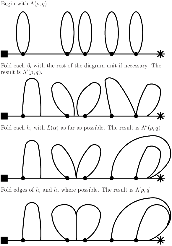
Proof.

It is clear from the definitions and the properties of diagram units (in particular Lemma 5.16 (2)) that there is a path $\tilde{\rho}^{\prime}_{kq}$ across $\Lambda^{\prime}(\rho,q)$ which is labelled by $f^{kq}_{\#}(\delta_{1})f^{kq}_{\#}(\delta_{2})\dots f^{kq}_{\#}(\delta_{s})$ and such that $k\mapsto l^{\rm{ab}}(\tilde{\rho}^{\prime}_{kq})$ is linear. By Remark 5.18, $\Lambda[\rho,q]$ is the immersion determined by $\Lambda^{\prime}(\rho,q)$ . It follows that Property (2) implies Property (1) and it remains only to show that Property (2) holds.

By the hypothesis that $\rho$ is in primary form with respect to $q$ , we may think of $\Lambda^{\prime}(\rho,q)$ as consisting of a line (corresponding to $L(\rho)$ ) with one handle (the part of $\Lambda[\delta_{i},q]$ not crossed by $\delta_{i}$ ) of length at least $q/2$ attached for each active growth unit. For growth units of type (LE) and (QE) there is no more folding possible between the corresponding handle and the line (since $h(\mu_{a})<a,b$ ). For growth units of type (LF) or (LR) there may be some further folding possible between the corresponding handle and the line. We examine the possibilities: suppose that $\delta_{i}$ is a growth unit of type (LF) for some integer $i$ such that $1\leq i\leq s$ and let $h_{i}$ denote the handle in $\Lambda^{\prime}(\rho,q)$ corresponding to $\delta_{i}$ . By construction, there is no folding possible between $h_{i}$ and the line-segment in $\Lambda^{\prime}(\rho,q)$ corresponding to $L(\delta_{1}\dots\delta_{i-1})$ , thus we may assume that $i<s$ . Let $L_{i+1}$ denote the line-segment in $\Lambda^{\prime}(\rho,q)$ corresponding to $L(\delta_{i+1}\dots\delta_{s})$ . Observe that $\hat{h}_{i}$ is a Nielsen path. If $\delta_{i+1}$ is a passive growth unit, less than $l(\delta_{i+1})\leq\lambda_{1}$ edges of $h_{i}$ may fold with $L_{i+1}$ (any further folding would violate the maximality condition in Step 3 of the separation algorithm). If $\delta_{i+1}$ has type (LE) or (QE), less than $\lambda_{1}$ edges of $h_{i}$ fold with $L_{i+1}$ (otherwise, $\hat{h}_{i}$ contains an essentially unbounded subpath $\hat{\delta}_{i+1}$ , which is impossible by Remark 3.10 (1)). Finally, consider the case that $\delta_{i+1}$ has type (LR). Since $\hat{h}_{i}$ is a Nielsen path, less than $l(\delta_{i+1})$ edges of $h_{i}$ fold with $L_{i+1}$ (otherwise, again, $\hat{h}_{i}$ contains an essentially unbounded subpath $\hat{\delta}_{i+1}$ ). It follows from Lemma 5.22 and the definition of growth units that, if $\lambda_{0}$ edges of $h_{i}$ fold with $L_{i+1}$ then $\delta_{i}\delta_{i+1}$ is a growth unit of type (FE), (LE) or (QE), contradicting Step 1 of the separation algorithm. Hence less than $\lambda_{0}$ edges of $h_{i}$ fold with $L_{i+1}$ . A similar examination of the possibilities in the case that $\delta_{i}$ has type (LR) allows us to conclude the following: after performing all folding possible between the handles and $L(\alpha)$ in $\Lambda^{\prime}(\rho,q)$ , the resulting graph $\Lambda^{\prime\prime}(\rho,q)$ may be viewed as a line with one handle attached for each active growth unit, where each such handle has length at least $q/2-\max\{\lambda_{1},\lambda_{0}\}$ .

There may be some folding possible between handles in $\Lambda^{\prime\prime}(\rho,q)$ . Suppose at least $\lambda_{0}$ edges of $h_{i}$ are identified with edges of $h_{j}$ in $\Lambda[\rho,q]$ , for some integers $i$ and $j$ such that $1\leq i<j\leq s$ . By Lemma 5.22, $B(\delta_{i},q)$ and $B(\delta_{j},q)$ are identified in $\Lambda[\rho,q]$ and hence $\delta_{i}\delta_{i+1}\dots\delta_{j}$ is a growth unit of type (FE),(LE) or (QE)) — a contradiction to the separation algorithm. Thus we have that less than $\lambda_{0}$ pairs of edges may fold between any two handles in $\Lambda^{\prime\prime}(\rho,q)$ and it follows from our hypothesis on $q$ that each handle contains at least one geometric edge which does not fold with any other handle. Thus Property (2) holds. ∎

Theorem 5.27.

The Apt Immersion Theorem holds in the case that $\sigma$ is a circuit with linear growth.

Proof.

Let $\rho$ be a well-chosen closed tight path representing $\sigma$ . Choose $q$ such that $q>2\max\{\lambda_{1},\lambda_{0}\}+4\lambda_{0}$ and $q>2l(\rho)$ so that we may apply Lemma 5.19 and Proposition 5.24 (1) to $\Lambda[\rho,q]$ . It follows immediately that $\Sigma[\rho,q]$ satisfies (AI1) and (AI2). ∎

Remark 5.28.

Although it would be unjustifiably distracting to develop the necessary ideas here, it can be shown that there exists a constant $q_{0}\in\mathbb{N}$ such that we may replace the hypothesis in Proposition 5.24 that $\rho$ is in primary form with respect to $q$ by the hypothesis that $q\geq q_{0}$ .

6. The Apt Immersion Theorem in the non-linear case

In the linear growth case we used growth units to write our path as a concatenation of subpaths which interact in a limited way under iteration of $f_{\#}$ ; in the non-linear case we introduce the notion of ‘path units’. Path units are analogous to basic paths but more flexible. A path $\rho$ of degree $d\geq 2$ $f$ -splits canonically into path units of degree $d$ and paths of degree at most $d-1$ , and hence we write $\rho$ as a concatenation of subpaths which do not interact at all under iteration of $f_{\#}$ . We assign to $\rho$ a description, called the ‘path unit structure’, which summarises this concatenation. Importantly, the path unit structure of a path is invariant under the action of $f_{\#}$ . Recognising this allows us to construct different end-pointed $G$ -immersions tailored for the different path units of $\rho$ , which can then be combined using our standard constructions. By taking care at the neighbourhood of each end-point of the $G$ -immersions constructed, we may ensure that no folding will be required when the $G$ -immersions are combined. In this way we reduce the task of proving the Apt Immersion Theorem to the task of constructing $G$ -immersions which carry and stretch path units (in the sense of Remark 4.2) and their $f^{q}_{\#}$ iterates and for which the neighbourhoods of the end-points are appropriately simple. We perform the necessary construction inductively, inducting on the degree $d$ and making repeated use of Stallings’ Algorithm and the structure of the IRTT representative $f:G\to G$ .

6.1. Path units

The following definition should be compared to that of a basic path ( $\lx@sectionsign$ 3.2).

Definition 6.1 (Path Units).

Let $n\geq 2$ be an integer. A path unit (of degree $d$ ) is a path $\alpha$ in $G$ in one of the following forms:

(i)

$e_{a}\gamma\overline{e}_{b}$ ;
(ii)

$e_{a}\gamma$ ; or
(iii)

$\gamma\overline{e}_{b}$ ,

where $a,b\in\mathbb{N}$ are such that $L_{d}\leq a,b<L_{d+1}$ and $\gamma$ is a path in $G_{L_{d}-1}$ . A path unit which has form $(t)$ for some $t\in\{i,ii,iii\}$ is said to have type (t).

Definition 6.2 (Canonical $f$ -splitting of a path).

Let $\rho$ in $G$ be a path. We define the canonical $f$ -splitting of $\rho$ as follows: if $h(\rho)<L_{1}$ , then the canonical $f$ -splitting is simply the path $\rho$ ; if $L_{1}\leq h(\rho)<L_{2}$ , then $f$ -split $\rho$ immediately before each occurrence of $e_{h(\rho)}$ and after each occurrence of $\overline{e}_{h(\rho)}$ ; if $L_{d}\leq h(\rho)<L_{d+1}$ for some $d\geq 2$ , then, for each integer $i$ such that $L_{d}\leq i<L_{d+1}$ , $f$ -split $\rho$ immediately before each occurrence of $e_{i}$ and after each occurrence of $\overline{e}_{i}$ .

Notation 6.3.

We denote that an $f$ -splitting $\rho=\alpha_{1}\cdot\alpha_{2}\cdot\dots\cdot\alpha_{s}$ is in fact the canonical $f$ -splitting by using the symbol $\ast$ between subpaths rather than the symbol $\cdot$ , that is, we write $\rho=\alpha_{1}\ast\alpha_{2}\ast\dots\ast\alpha_{s}$ .

Remark 6.4.

If $\rho$ has degree $d\geq 2$ , the canonical $f$ -splitting writes $\rho$ as a concatenation of maximal path units of degree $d$ and paths of degree at most $d-1$ . If $\rho$ is linear, the canonical $f$ -splitting writes $\rho$ as a concatenation of maximal basic paths of height $h(\rho)$ and paths of height at most $h(\rho)-1$ .

The following lemma is an immediate consequence of Property (TT4) of the IRTT Theorem.

Lemma 6.5.

Let $\alpha\subset G$ be a path unit. If $\alpha$ has type (i) then $f_{\#}(\alpha)$ and $\overline{f}_{\#}(\alpha)$ are path units of type (i) with the same initial and terminal edges as $\alpha$ ; if $\alpha$ has type (ii) then $f_{\#}(\alpha)$ and $\overline{f}_{\#}(\alpha)$ are path units of type (ii) with the same initial edge as $\alpha$ ; if $\alpha$ has type (iii) then $f_{\#}(\alpha)$ and $\overline{f}_{\#}(\alpha)$ are path units of type (iii) with the same terminal edge as $\alpha$ .

Remark 6.6.

Let $\alpha\subset G$ be a path unit. We define the structure of $\alpha$ , denoted ${\rm str}(\alpha)$ as follows: if $\alpha=e_{a}\gamma\overline{e}_{b}$ has type (i) then ${\rm str}(\alpha)=((i),a,b)$ ; if $\alpha=e_{a}\gamma$ has type (ii) then ${\rm str}(\alpha)=((ii),a)$ ; if $\alpha=\gamma\overline{e}_{b}$ has type (iii) then ${\rm str}(\alpha)=((iii),b)$ . For a path $\rho=\alpha_{1}\ast\alpha_{2}\ast\dots\ast\alpha_{s}$ in $G$ of degree $d$ , define the path unit structure of $\rho$ to be a finite list of sets $s_{1},s_{2},\dots,s_{s}$ , where $s_{i}=\emptyset$ if degree $\alpha_{i}<d$ , otherwise $s_{i}:={\rm str}(\alpha_{i})$ . It is an immediate corollary to Lemma 6.5 that the path unit structure of a path is invariant under the action of $f_{\#}$ and $\overline{f}_{\#}$ .

6.2. Tails of edges

Let $a\geq 1$ be an integer. We now investigate the structure of the ‘ $f$ -tails’ of $e_{a}$ , that is, the infinite paths $S_{a}^{+}$ and $S_{a}^{-}$ such that $f^{k}_{\#}(e_{a})\to e_{a}S_{a}^{+}$ and $\overline{f}^{k}_{\#}(e_{a})\to e_{a}S_{a}^{-}$ as $k\to\infty$ . An understanding of this structure is crucial for building $G$ -immersions which carry a path unit which crosses $E_{a}$ .

For each integer $a$ such that $L_{1}\leq a<h(G)$ , define an infinite tight path $S^{+}_{a}:=u_{a}f_{\#}(u_{a})f^{2}_{\#}(u_{a})\dots$ . We define a second infinite tight path $S^{-}_{a}$ in one of two ways, depending on whether $u_{a}$ is a well-chosen closed tight path or not:

In the case that $u_{a}$ is a well-chosen closed tight path, let $u_{a}=\epsilon_{a,\,0}\ast\epsilon_{a,\,1}\ast\dots\ast\epsilon_{a,s_{a}-1}$ . Note that

S^{+}_{a}=\epsilon_{a,\,0}\ast\epsilon_{a,\,1}\ast\dots\ast\epsilon_{a,s_{a}-1}\ast f_{\#}(\epsilon_{a,\,0})\ast f_{\#}(\epsilon_{a,\,1})\ast\dots\ast f_{\#}(\epsilon_{a,s_{a}-1})\ast\dots.

Define an infinite tight path,

S^{-}_{a}:=\overline{f}_{\#}(\overline{\epsilon}_{a,\,s_{a}-1})\ast\dots\ast\overline{f}_{\#}(\overline{\epsilon}_{a,\,0})\ast\overline{f}^{2}_{\#}(\overline{\epsilon}_{a,\,s_{a}-1})\ast\dots\ast\overline{f}^{2}_{\#}(\overline{\epsilon}_{a,\,0})\ast\dots.

In the case that $u_{a}$ is not a well-chosen closed tight path, let $u_{a}=\epsilon^{\prime}_{a,\,0}\ast\epsilon_{a,\,1}\ast\dots\ast\epsilon_{a,s_{a}-1}\ast\epsilon^{\prime}_{a,\,s_{a}}$ and define $\epsilon_{a,\,0}:=[\overline{f}_{\#}(\epsilon^{\prime}_{a,\,s_{a}})\epsilon^{\prime}_{a,\,0}]$ . Note that

S^{+}_{a}=\epsilon^{\prime}_{a,\,0}\ast\epsilon_{a,\,1}\ast\dots\ast\epsilon_{a,s_{a}-1}\ast f_{\#}(\epsilon_{a,\,0})\ast f_{\#}(\epsilon_{a,\,1})\ast\dots\ast f_{\#}(\epsilon_{a,s_{a}-1})\ast\dots.

Define an infinite tight path,

S^{-}_{a}:=\overline{f}_{\#}(\overline{\epsilon}^{\prime}_{a,\,s_{a}})\ast\overline{f}_{\#}(\overline{\epsilon}_{a,\,s_{a}-1})\ast\dots\ast\overline{f}_{\#}(\overline{\epsilon}_{a,\,0})\ast\overline{f}^{2}_{\#}(\overline{\epsilon}_{a,\,s_{a}-1})\ast\dots\ast\overline{f}^{2}_{\#}(\overline{\epsilon}_{a,\,0})\ast\dots.

In either case, observe that

\begin{split}[\overline{S_{a}^{-}}S_{a}^{+}]=\dots\ast\overline{f}_{\#}(\epsilon_{a,\,0})\ast\dots&\ast\overline{f}_{\#}(\epsilon_{a,\,s_{a}-1})\ast\epsilon_{a,\,0}\ast\dots\\ &\ast\epsilon_{a,\,s_{a}-1}\ast f_{\#}(\epsilon_{a,\,0})\ast\dots\ast f_{\#}(\epsilon_{a,\,s_{a}-1})\ast\dots.\end{split}

Notation 6.7.

For each integer $a$ such that $L_{1}\leq a<h(G)$ , relabel the canonical $f$ -splitting $S_{a}^{+}=\alpha_{a,\,0}\ast\alpha_{a,\,1}\ast\alpha_{a,\,2}\ast\dots$ and $S_{a}^{-}=\beta_{a,\,0}\ast\beta_{a,\,1}\ast\beta_{a,\,2}\ast\dots$ .

Remark 6.8.

For each $a\geq L_{2}$ and each integer $i\geq 1$ , $\alpha_{a,\,i+s_{a}}=f_{\#}(\alpha_{a,\,i})$ and $\beta_{a,\,i+s_{a}}=\overline{f}_{\#}(\beta_{a,\,i})$ .

Recall, in $\lx@sectionsign$ 4.2 we defined $\mu_{i}$ to be the primitive closed path corresponding to $u_{i}$ , for each integer $i$ such that $L_{1}\leq i<L_{2}$ .

Lemma 6.9 (The Linear Balloon Lemma).

Let $a,b\in\mathbb{N}$ be such that $L_{1}\leq a,b<L_{2}$ and define $K:=l(\mu_{a})l(\mu_{b})$ . The following properties hold:

(1)

if there exist finite tight paths $\rho_{1},\rho^{\prime}_{1},\rho_{2}$ and infinite tight paths $\rho_{3}$ and $\rho^{\prime}_{3}$ such that $S_{a}^{+}=\rho_{1}\rho_{2}\rho_{3}$ , $S_{b}^{+}=\rho^{\prime}_{1}\rho_{2}\rho^{\prime}_{3}$ and $l(\rho_{2})\geq K$ , then $\mu_{a}=\mu_{b}$ .
(2)

if there exist finite tight paths $\rho_{1},\rho^{\prime}_{1},\rho_{2}$ and infinite tight paths $\rho_{3}$ and $\rho^{\prime}_{3}$ such that $S_{a}^{+}=\rho_{1}\rho_{2}\rho_{3}$ , $S_{b}^{-}=\rho^{\prime}_{1}\rho_{2}\rho^{\prime}_{3}$ and $l(\rho_{2})\geq K$ , then $\mu_{a}$ is a cyclic permutation of $\overline{\mu}_{b}$ .

Proof.

Assume the hypothesis of Property (2). The infinite paths $S_{a}^{+},S_{a}^{-}$ are periodic with period $l(\mu_{a})$ and the infinite paths $S_{b}^{+},S_{b}^{-}$ are periodic with period $l(\mu_{b})$ . The periodicity of $S_{a}^{+}$ and $S_{b}^{-}$ imply that $l(\mu_{a})=l(\mu_{b})$ and $\mu_{a}$ is a cyclic permutation of $\overline{\mu}_{b}$ . That is, Property (2) holds.

Assume the hypothesis of Property (1). As above, the periodicity of $S_{a}^{+}$ and $S_{b}^{+}$ imply that $\mu_{a}$ is a cyclic permutation of $\mu_{b}$ . Suppose $\mu_{a}\neq\mu_{b}$ , say $\mu_{a}=\epsilon\mu_{b}\overline{\epsilon}$ . Then $e_{a}\epsilon\overline{e}_{b}$ is a tight path which violates (TT4) of the IRTT theorem. Thus $\mu_{a}=\mu_{b}$ and Property (1) holds. ∎

Lemma 6.9 is a consequence of the periodicity of $S^{+}_{a}$ and $S^{-}_{a}$ in the case that $L_{1}\leq a<L_{2}$ . In the case that $a\geq L_{2}$ , $S^{+}_{a}$ and $S^{-}_{a}$ are not periodic, but Remark 6.8 can be used to mimic the role of periodicity.

Lemma 6.10 (The Non-Linear Balloon Lemma).

Let $d\geq 2$ , let $a,b\in\mathbb{N}$ be such that $L_{d}\leq a,b<L_{d+1}$ and define $K:=s_{a}s_{b}+\min\{s_{a},s_{b}\}+1$ . The following properties hold:

(1)

if there exist finite tight paths $\rho_{1},\rho^{\prime}_{1},\rho_{2}$ and infinite tight paths $\rho_{3}$ and $\rho^{\prime}_{3}$ such that $S_{a}^{+}=\rho_{1}\rho_{2}\rho_{3}$ , $S_{b}^{+}=\rho^{\prime}_{1}\rho_{2}\rho^{\prime}_{3}$ and the separation of $\rho_{2}$ contains at least $K$ complete path units of the canonical $f$ -splitting of $S_{a}^{+}$ , then $a=b$ , $\rho^{\prime}_{1}=\rho_{1}$ and $\rho^{\prime}_{3}=\rho_{3}$ .
(2)

if there exist finite tight paths $\rho_{1},\rho^{\prime}_{1},\rho_{2}$ and infinite tight paths $\rho_{3}$ and $\rho^{\prime}_{3}$ such that $S_{a}^{-}=\rho_{1}\rho_{2}\rho_{3}$ , $S_{b}^{-}=\rho^{\prime}_{1}\rho_{2}\rho^{\prime}_{3}$ and the separation of $\rho_{2}$ contains at least $K$ complete path units of the canonical $f$ -splitting of $S_{a}^{-}$ , then $a=b$ , $\rho^{\prime}_{1}=\rho_{1}$ and $\rho^{\prime}_{3}=\rho_{3}$ .
(3)

if there exist finite tight paths $\rho_{1},\rho^{\prime}_{1},\rho_{2}$ and infinite tight paths $\rho_{3}$ and $\rho^{\prime}_{3}$ such that $S_{a}^{+}=\rho_{1}\rho_{2}\rho_{3}$ and $S_{b}^{-}=\rho^{\prime}_{1}\rho_{2}\rho^{\prime}_{3}$ , then the separation of $\rho_{2}$ contains less than $K$ complete path units of the canonical $f$ -splitting of $S_{a}^{+}$ .

Proof.

We first claim that the hypothesis of Property (1) implies that $s_{a}=s_{b}$ . The hypothesis implies that there exist $i,j\geq 1$ such that $\alpha_{a,\,i}\dots\alpha_{a,\,i+K-1}=\alpha_{b,\,j}\dots\alpha_{b,\,j+K-1}$ . Thus $\alpha_{a,\,i+s_{a}s_{b}+j}=f^{s_{b}}_{\#}(\alpha_{a,\,i+j})=f^{s_{a}}_{\#}(\alpha_{a,\,i+j})$ , for $j=0$ , $1$ , $\dots$ , $\min\{s_{a},s_{b}\}-1$ (by Remark 6.8). But at least one of the path units $\alpha_{a,i+j}$ is not a Nielsen path, say $j=j_{0}$ , and $f^{s_{b}}_{\#}(\alpha_{a,\,i+j_{0}})=f^{s_{a}}_{\#}(\alpha_{a,\,i+j_{0}})$ implies that $s_{a}=s_{b}$ .

Now, suppose that the path $\alpha=[e_{a}\alpha_{a,\,0}\dots\alpha_{a,\,i-1}\overline{\alpha}_{b,\,j-1}\dots\overline{\alpha}_{b,\,0}\overline{e}_{b}]$ is not the trivial path. We may assume that $\alpha=e_{a}\alpha_{a,\,0}\dots[\alpha_{a,\,i-1}\overline{\alpha}_{b,\,j-1}]\dots\overline{\alpha}_{b,\,0}\overline{e}_{b}$ . Then

$\displaystyle f_{\#}(\alpha)$	$\displaystyle=$	$\displaystyle[e_{a}\alpha_{a,\,0}\dots\alpha_{a,\,i-1}\alpha_{a,\,i}\dots\alpha_{a,\,i+s_{a}-1}\overline{\alpha}_{b,\,j+s_{b}-1}\dots\overline{\alpha}_{b,\,j}\overline{\alpha}_{b,\,j-1}\dots\overline{\alpha}_{b,\,0}\overline{e}_{b}]$
	$\displaystyle=$	$\displaystyle e_{a}\alpha_{a,\,0}\dots[\alpha_{a,\,i-1}\alpha_{a,\,i}\dots\alpha_{a,\,i+s_{a}-1}\overline{\alpha}_{a,\,i+s_{a}-1}\dots\overline{\alpha}_{a,\,i}\overline{\alpha}_{b,\,j-1}]\dots\overline{\alpha}_{b,\,0}\overline{e}_{b}$
	$\displaystyle=$	$\displaystyle e_{a}\alpha_{a,\,0}\dots[\alpha_{a,\,i-1}\overline{\alpha}_{b,\,j-1}]\dots\overline{\alpha}_{b,\,0}\overline{e}_{b}.$

Hence $\alpha$ is a Nielsen path which crosses a non-linear edge — a contradiction to the Corollary 3.16 (4). Thus $\alpha$ is the trivial path, and the conclusions of Property (1) hold.

Property (2) may be proved by a similar argument to the above.

Assume the hypothesis of Property (3). Suppose that the separation of $\rho_{2}$ contains at least $K$ complete path units of the canonical $f$ -splitting of $S_{a}^{+}$ . By hypothesis, there exist $i,j\in\mathbb{N}$ such that $\alpha_{a,\,i}\dots\alpha_{a,\,i+K-1}=\beta_{b,\,j}\dots\beta_{b,\,j+K-1}$ . Thus $\alpha_{a,\,i+s_{a}s_{b}+j}=f^{s_{b}}_{\#}(\alpha_{a,\,i+j})=\overline{f}^{s_{a}}_{\#}(\alpha_{a,\,i+j})$ , for $j=0,1,\dots,\min\{s_{a},s_{b}\}-1$ . This implies that each $\alpha_{a,\,i+j}$ is a Nielsen path, a contradiction to the fact that $a\geq L_{d}\geq L_{2}$ . Hence Property (2) holds. ∎

Lemma 6.11.

For each $a\in\mathbb{N}$ such that $a\geq L_{2}$ and for each non-negative integer $k$ , the infinite paths $\alpha_{a,\,k}\alpha_{a,\,k+1}\dots$ and $\beta_{a,\,k}\beta_{a,\,k+1}\dots$ each contain an essentially unbounded subpath.

Proof.

Immediate by Lemma 5.12. ∎

6.3. A strategy of proof

In this section we indicate our strategy for completing the proof of the Apt Immersion Theorem.

Lemma 6.12.

Let $\alpha\subset G$ be a path unit. There exists an end-pointed $G$ -immersion $\Gamma$ with the following properties:

(1)

$\iota(\Gamma)\neq\tau(\Gamma)$ ;
(2)

if $\alpha$ has type (i) then both $\iota(\Gamma)$ and $\tau(\Gamma)$ have valence 1; if $\alpha$ has type (ii) then $\iota(\Gamma)$ has valence 1; if $\alpha$ has type (iii) then $\tau(\Gamma)$ has valence 1;
(3)

$\Gamma$ is $f$ -stable;
(4)

$\alpha$ labels a path across $\Gamma$ .

Proof.

Consider the case that $\alpha$ has type (i), say, $\alpha=e_{a}\gamma\overline{e}_{b}$ . Let $d$ be such that $L_{d}\leq h(\alpha)<L_{d+1}$ and let $G^{\prime}$ be the connected component of $G_{L_{d}-1}$ containing $\gamma$ . Extend $L(\gamma)$ to a $G^{\prime}$ -cover $P$ . Define the initial and terminal points of $P$ to be those corresponding to the initial and terminal points of $L(\gamma)$ respectively. Define $\Gamma:=\vee((L(e_{a}),P,L(\overline{e}_{b}))$ . Properties (1), (2) and (4) are immediate by construction. Property (3) follows easily from the construction and the fact that $\mu_{a},\mu_{b}\subset G^{\prime}$ . An upper bound on $period(\Gamma)$ is given by $\left|\mathcal{V}_{\Gamma}\right|!$ . The cases that $\alpha$ has type (ii) and type (iii) are proved similarly. ∎

Sketch of a proof of the Apt Immersion Theorem in the non-linear case.

Let $\sigma\subset G$ be a circuit of degree $d$ and let $\rho=\alpha_{1}\ast\alpha_{2}\ast\dots\ast\alpha_{s}$ be a well-chosen closed tight path corresponding to $\sigma$ . For each $i=1,2,\dots,s,$ there exists an end-pointed $G$ -immersion $\Gamma_{i}$ which satisfies the conclusions of Lemma 6.12 for $\alpha_{i}$ . For each $i=1,2,\dots,s$ , let $q_{i}={{\rm period}_{f}}(\Gamma_{i})$ . Define $q={\rm lcm}\{q_{i}\hbox{ }|\hbox{ }1\leq i\leq s\}$ and $\Gamma:=\vee^{\circlearrowleft}(\Gamma_{1},\dots,\Gamma_{s}).$ Properties (1) and (2) of Lemma 6.12 imply that $\Gamma$ is a $G$ -immersion. Properties (3) and (4) of Lemma 6.12 imply that, for each non-negative integer $k$ , $f^{kq}_{\#}(\rho)$ labels a path across $\Gamma$ . Further, since $f^{kq}_{\#}(\rho)=f^{kq}_{\#}(\alpha_{1})\ast f^{kq}_{\#}(\alpha_{2})\ast\dots\ast f^{kq}_{\#}(\alpha_{s})$ for each non-negative integer $k$ , $f^{kq}_{\#}(\alpha_{i})$ labels a path across $\Gamma_{i}\subset\Gamma$ . Since $\rho$ is a well-chosen closed tight path, either the initial edge of $\rho$ is $e_{h(\rho)}$ or the terminal edge of $\rho$ is $\overline{e}_{h(\rho)}$ . Without loss of generality, we may assume that the former case holds. Let $\tilde{\alpha}_{1,\,k}$ be the path across $\Gamma_{1}$ labelled by $f^{kq_{1}}_{\#}(\alpha_{1})$ . If we can ensure that $\Gamma_{1}$ is such that $k\mapsto l^{\rm{ab}}(\tilde{\alpha}_{1,\,k})$ is an element of $p_{d}$ , then $\Gamma$ and $q$ will satisfy the conclusions of the Apt Immersion Theorem (and the proof of the Main Theorem will be complete). ∎

6.4. The Periodic Open Immersions Lemma

Next we use a simple finiteness argument to find, for a path unit $\alpha$ in $G$ , a periodic sequence of end-pointed $G$ -immersions $\{\Gamma_{i}\}_{i\in\mathbb{N}}$ with Properties (1) and (2) of Lemma 6.12 and such that $\Gamma_{i}$ carries $f^{i}_{\#}(\alpha)$ . The periodicity of the sequence is crucial because it allows us to join finite strings of such end-pointed $G$ -immersions into base-pointed $G$ -immersions such that, for some integer $a\geq L_{2}$ and some $q\in\mathbb{N}$ , the result carries $S^{+}_{a}$ and $S^{-}_{a}$ .

Lemma 6.13.

Let $\alpha\subset G$ be a path unit of degree $d\geq 2$ . There exist $m,r\in\mathbb{N}$ and a finite set of end-pointed $G$ -immersions $\{\Gamma_{0},\dots,\Gamma_{r-1}\}$ such that, for each $i=0,1,\dots,r-1$ and each $j=0,1,\dots,m-1$ , the following properties hold:

(1)

$\iota(\Gamma_{i})\neq\tau(\Gamma_{i})$ ;
(2)

if $\alpha$ has type (i) then both $\iota(\Gamma_{i})$ and $\tau(\Gamma_{i})$ have valence 1; if $\alpha$ has type (ii) then $\iota(\Gamma_{i})$ has valence 1; if $\alpha$ has type (iii) then $\tau(\Gamma_{i})$ has valence 1;
(3)

$\Gamma_{i}$ is $f$ -stable and ${{\rm period}_{f}}(\Gamma_{i})$ divides $m$ ;
(4)

there exist $i_{j}\in\{0,1,\dots,r-1\}$ such that $f^{j}_{\#}(\alpha)$ labels a path across $\Gamma_{i_{j}}$ .

Proof.

Let $a=h(\alpha)$ , let $d$ be such that $L_{d}\leq h(\alpha)<L_{d+1}$ and assume, without loss of generality, that the initial edge of $\alpha$ is $e_{a}$ (that is, $\alpha$ has type (i) or type (ii)). Let $G^{\prime}$ be the connected component of $G_{a}$ which contains $e_{a}$ and let $H=\pi_{1}(G^{\prime},\iota(e_{a}))$ . If $\alpha$ has type (ii), the result holds with $r=1$ , $m=1$ and $(\Gamma_{0},p_{0})$ constructed from $G^{\prime}$ simply by detaching the initial point of $e_{a}$ . Thus we may assume that $\alpha$ has type (i), that is, $\alpha=e_{a}\gamma\overline{e}_{b}$ for some $b\in\mathbb{N}$ such that $L_{d}\leq b\leq a$ and for some $\gamma\subset G_{L_{d}-1}$ . If $a\neq b$ , the result holds with $r=1$ , $m=1$ and $(\Gamma_{0},p_{0})$ constructed from $G^{\prime}$ simply by detaching the initial point of $e_{a}$ and the initial point $e_{b}$ . Thus we may assume that $a=b$ .

Because free groups are residually finite, there exists a finite-index subgroup $H_{0}\leq H$ such that $\hat{\alpha}\not\in H_{0}$ ; write $I:=[H:H_{0}]$ . Now $H$ is $\phi$ -invariant and $\phi|_{H}$ permutes the set of subgroups of $H$ of index $I$ . Let $\{H_{0},H_{1},\dots,H_{s-1}\}$ be the $\phi|_{H}$ -orbit of $H_{0}$ (indexed such that $(\phi|_{H})^{k}(H_{0})=H_{k\,\rm{mod}\,s}$ ). For each $i=0,1,\dots,s-1$ , let $(\Delta^{\prime}_{i},p^{\prime}_{i})$ be a $G^{\prime}$ -cover and let $\tilde{b}_{i}\in\Delta_{i}$ be a vertex such that ${p^{\prime}_{i}}(\tilde{b}_{i})=\iota(e_{a})$ and ${p^{\prime}_{i}}_{\ast}\pi_{1}(\Delta^{\prime}_{i},\tilde{b}_{i})$ corresponds to $H_{i}$ . Let $(\Delta_{i},p_{i})$ be constructed from $(\Delta^{\prime}_{i},p^{\prime}_{i})$ by detaching each edge with label $e_{a}$ at the initial point. Let $\tilde{c}_{i}^{0},\tilde{c}_{i}^{1},\dots,\tilde{c}_{i}^{I-1}$ be an enumeration of the vertices in $(p_{i})^{-1}(\iota(e_{a}))$ such that $\tilde{c}_{i}^{0}$ corresponds to $\tilde{b}_{i}$ . For each $j=1,2,\dots,I-1$ , let $(\Delta_{i}^{j},p_{i}^{j})$ be the end-pointed $G_{i}$ -labelled graph $(\Delta_{i},p_{i})$ with initial point $\tilde{c}_{i}^{0}$ and terminal point $\tilde{c}_{i}^{j}$ .

Now, $\alpha\not\in H_{0}$ implies that, for each non-negative integer $j$ , $f^{j}_{\#}(\alpha)\not\in H_{j\,\rm{mod}\,s}$ . Hence $f^{j}_{\#}(\alpha)$ lifts to an open path in $\Delta^{\prime}_{j\,\rm{mod}\,s}$ at $\tilde{b}_{j\,\rm{mod}\,s}$ . It follows that $f^{k}j_{\#}(\alpha)$ labels a path across $\Delta_{j\,\rm{mod}\,s}^{l}$ for some integer $l$ such that $1\leq l\leq I-1$ . Since any lift of $(f|_{G^{\prime}})^{I!}$ to $\Delta^{\prime}_{i}$ fixes each vertex of $\Delta^{\prime}_{i}$ , for each non-negative integer $k$ , we know that $f^{j+k(I!)}_{\#}(\alpha)$ labels a path across $\Delta_{j\,\rm{mod}\,s}^{l}$ . Thus the result holds, with $m=I!$ , $r=sI$ , and $\{(\Gamma_{0},p_{0}),\dots,(\Gamma_{r-1},p_{r-1})\}=\{(\Delta_{i}^{j},p^{i}_{j})\hbox{ }|\hbox{ }0\leq i<s;1\leq j<I\}$ . ∎

The following corollary to Lemma 6.13 is obtained by replacing the set of $G$ -immersions by an ordered list of $G$ -immersions.

Corollary 6.14 (The Periodic Open Immersions Lemma).

Let $\alpha_{1},\dots,\alpha_{s}\subset G$ be a finite ordered list of path units of degree $d\geq 2$ . There exists $q\in\mathbb{N}$ and, for each $i=1,2,\dots,s$ , there exists a finite list of end-pointed $G$ -immersions $\Gamma_{i}^{0},\dots,\Gamma_{i}^{q-1},$ such that, for each $j=0,1,\dots,q-1$ , the following properties hold:

(1)

$\iota(\Gamma_{i}^{j})\neq\tau(\Gamma_{i}^{j})$ ;
(2)

if $\alpha_{i}$ has type (i) then both $\iota(\Gamma_{i}^{j})$ and $\tau(\Gamma_{i}^{j})$ have valence 1; if $\alpha_{i}$ has type (ii) then $\iota(\Gamma_{i}^{j})$ has valence 1; if $\alpha_{i}$ has type (iii) then $\tau(\Gamma_{i}^{j})$ has valence 1;
(3)

$\Gamma_{i}^{j}$ is $f$ -stable with ${{\rm period}_{f}}(\Gamma_{i}^{j})\,|\,q$ ; and
(4)

$f^{j}_{\#}(\alpha_{i})$ labels a path across $\Gamma_{i}^{j}$ .

Remark 6.15.

For each $i=1,2,\dots,s$ , consider the periodic bi-infinite sequence of end-pointed $G$ -immersions $\{\Gamma_{i}^{k}\}_{k\in\,\mathbb{Z}}$ , where for $k<0$ and $k\geq q$ , $\Gamma_{i}^{k}:=\Gamma_{i}^{k\,\rm{mod}\,q}$ . Properties (3) and (4) imply that $\alpha_{i}$ labels a path across $\Gamma_{i}^{0}$ and, for each $k\in\mathbb{N}$ , $f^{k}_{\#}(\alpha_{i})$ labels a path across $\Gamma_{i}^{k}$ and $\overline{f}^{k}_{\#}(\alpha_{i})$ labels a path across $\Gamma_{i}^{-k}$ .

6.5. The Apt Immersion Theorem in the quadratic case

The following completes the proof of the Apt Immersion Theorem in the quadratic case and hence completes the proof of the Main Theorem in the case that $\mathcal{G}_{\phi}\in p_{2}$ .

Proposition 6.16.

Let $\alpha\subset G$ be a path unit of degree 2. There exists an end-pointed $G$ -immersion $\Sigma$ such that the following conditions hold:

$(\Sigma 1)$

$\iota(\Sigma)\neq\tau(\Sigma)$ ;
$(\Sigma 2)$

If $\alpha$ has type (i) then both $\iota(\Sigma)$ and $\tau(\Sigma)$ have valence 1; if $\alpha$ has type (ii) then $\iota(\Sigma)$ has valence 1; if $\alpha$ has type (iii) then $\tau(\Sigma)$ has valence 1;
$(\Sigma 3)$

For each non-negative integer $k$ , $f^{kq}_{\#}(\alpha)$ labels a path $\tilde{\alpha}_{kq}$ across $\Sigma$ ;
$(\Sigma 4)$

$k\mapsto l^{\rm{ab}}(\tilde{\alpha}_{kq})$ is an element of $p_{2}$ .

Proof.

Consider the case that $\alpha$ has type (i) (the hardest case). Suppose that $\alpha$ has type (i), say $\alpha=e_{a}\alpha^{\prime}\overline{e}_{b}$ , and consider $h(u_{a})$ , $h(u_{b})$ and $h(\alpha^{\prime})$ . We may assume, without loss of generality, that $h(u_{a})\geq h(u_{b})$ . The case that $h(u_{a})=h(u_{b})\geq h(\alpha^{\prime})$ is Lemma 6.17; the case that $h(u_{a})>h(u_{b})$ and $h(u_{a})\geq h(\alpha^{\prime})$ is Lemma 6.19; the case that $h(\alpha^{\prime})>h(u_{a})=h(u_{b})$ is Lemma 6.21; the case that $h(\alpha^{\prime})>h(u_{a})>h(u_{b})$ is Lemma 6.23. The proof in the case that $\alpha$ has type (ii) is performed similarly. By considering $\overline{\alpha}$ instead of $\alpha$ , it is clear that the case that $\alpha$ has type (iii) is equivalent to the case that $\alpha$ has type (ii). ∎

Lemma 6.17.

Proposition 6.16 holds in the case that $\alpha=e_{a}\alpha^{\prime}\overline{e}_{b}$ and $h(u_{a})=h(u_{b})\geq h(\alpha^{\prime})$ .

Proof.

(An example construction of $\Sigma$ as below is illustrated schematically in Figure 6.18). Define $h:=h(u_{a})$ , $K:=s_{a}s_{b}+\min\{s_{a},s_{b}\}+1$ and $l:=l(\alpha^{\prime})+2K+1$ . Let $U_{a}^{+}$ (respectively, $U_{a}^{-},U_{b}^{+},U_{b}^{-}$ ) be the initial subpath of $S_{a}^{+}$ (respectively, $S_{a}^{-},S_{b}^{+},S_{b}^{-}$ ) consisting of the first $l$ path units in the canonical $f$ -splitting. Let $d_{a}\in\mathcal{E}_{L(\alpha)}$ (respectively, $d_{b}\in\mathcal{E}_{L(\alpha)}$ ) be the unique edge in $L(\alpha)$ labelled by $e_{a}$ (respectively, $e_{b}$ ). Define an end-pointed $G$ -labelled graph

T^{\prime}:=L(\alpha)\amalg L(U_{a}^{+})\amalg L(U_{a}^{-})\amalg L(U_{b}^{+})\amalg L(U_{b}^{-})/\sim,

where $\sim$ equates $\tau(d_{a})$ , $\iota(L(U_{a}^{+}))$ and $\iota(L(U_{a}^{-}))$ and equates $\tau(d_{b})$ , $\iota(L(U_{b}^{+}))$ and $\iota(L(U_{b}^{-}))$ . Define the end-points of $T^{\prime}$ to be the image of the end-points of $L(\alpha)$ . Define $T$ to be the end-pointed $G$ -immersion determined by $T^{\prime}$ . Let $v_{a}$ (respectively, $v_{a}^{\pm},v_{b},v_{b}^{\pm}$ ) denote the image of $\tau(d_{a})$ (respectively, $\tau(L(U_{a}^{\pm}))$ , $\tau(d_{b})$ , $\tau(L(U_{b}^{\pm}))$ ) in $T$ .

Suppose at least $K$ edges of $U_{a}^{+}$ and $U_{b}^{+}$ become identified in $T$ . By Lemma 6.10 (1), $\mu_{a}=\mu_{b}$ and $\alpha^{\prime}=\mu_{a}^{k}$ for some $k\in\mathbb{Z}$ . Thus, $\alpha$ is an exceptional path — a contradiction to Corollary 3.16 (4). Similarly, the folding between any pair from the set $\{U_{a}^{+},U_{a}^{-},U_{b}^{+},U_{b}^{-}\}$ is limited by Lemma 6.10. Hence the definition of $l$ implies that the following properties hold:

•

$T$ is a tree with six distinct ends; and
•

the six end-paths (see Definition 2.9) have labels $e_{a},e_{b},\epsilon_{a}^{+},\epsilon_{a}^{-},\epsilon_{b}^{+},\epsilon_{b}^{-}$ such that each of $\epsilon_{a}^{+},\epsilon_{a}^{-},\epsilon_{b}^{+},\epsilon_{b}^{-}$ crosses $E_{h(u_{a})}$ .

Construct a $G$ -immersion $T^{\ast}$ from $T$ by extending each connected component of $p^{-1}(G_{h-1})$ to a connected $G_{h-1}$ -covering (if an end-path of $T$ has label $\overline{e}_{h}$ , then adjoin a $G_{h-1}$ cover at the corresponding end of $T$ ). It follows immediately from (TT3) of the IRTT Theorem that the following properties hold:

(A)

$T^{\ast}\setminus\{D_{a},D_{b}\}$ is $f$ -stable with period $q_{0}$ , say.
(B)

$\alpha_{a,\,0}\dots\alpha_{a,\,l-1}$ labels a path from $v_{a}$ to $v_{a}^{+}$ ;
$\overline{\beta}_{a,\,l-1}\dots\overline{\beta}_{a,\,0}$ labels a path from $v_{a}^{-}$ to $v_{a}$ ;
$\alpha_{b,\,0}\dots\alpha_{b,\,l-1}$ labels a path from $v_{b}$ to $v_{b}^{+}$ ;
$\overline{\beta}_{b,\,l-1}\dots\overline{\beta}_{b,\,0}$ labels a path from $v_{b}^{-}$ to $v_{b}$ ;
$\alpha^{\prime}$ labels a path from $v_{a}$ to $v_{b}$ .

By Proposition 5.24, for sufficiently large $q_{1}\in\mathbb{N}$ , the following property holds:

By the Periodic Open Immersions Lemma (applied to $\alpha_{a,\,1}$ , $\dots$ , $\alpha_{a,\,s_{a}}$ ), there exist $q_{2}\in\mathbb{N}$ and a bi-infinite sequence of end-pointed $G$ -immersions $\{\Gamma_{a,\,i}\}_{i\in\,\mathbb{Z}}$ such that the following properties hold for each $i\in\mathbb{Z}$ :

(D)

Properties (1) and (2) of the Periodic Open Immersions Lemma are satisfied;
(E)

$\Gamma_{a,\,i}$ is $f$ -stable with ${{\rm period}_{f}}(\Gamma_{a,\,i})\,|\,q_{2}$ ;
(F)

$\alpha_{a,\,i}$ labels a path across $\Gamma_{a,\,i}$ .

Similarly, there exist $q_{3}\in\mathbb{N}$ and $\{\Gamma_{b,\,i}\}_{i\in\,\mathbb{Z}}$ such that properties (D’), (E’) and (F’), analogous to (D), (E) and (F) respectively, hold. Choose $m\in\mathbb{N}$ such that $q:=mq_{0}q_{1}q_{2}q_{3}s_{a}s_{b}>2l+1$ . Define end-pointed $G$ -labelled graphs $L_{a}:=\vee(\Gamma_{a,\,l+1},\Gamma_{a,\,l+2},\dots,\Gamma_{a,\,q-l-2})$ and $L_{b}:=\vee(\Gamma_{b,\,l},\Gamma_{b,\,l+1},\dots,\Gamma_{b,\,q-l-2}).$ Properties (D) and (D’) imply that $L_{a}$ and $L_{b}$ are end-pointed $G$ -immersions. Properties (A), (B), (E), (F), (E’) and (F’) imply that, for each $k\in\mathbb{Z}$ ,

(G)

$f^{kq}_{\#}(\alpha_{a,\,0}\dots\alpha_{a,\,l-1})$ labels a path from $v_{a}$ to $v_{a}^{+}$ ;
$f^{kq}_{\#}(\alpha_{a,\,l})$ labels a path $\tilde{\beta}_{kq}$ across $\Lambda$ such that $k\mapsto l^{\rm{ab}}(\tilde{\beta}_{kq})\in p_{d-1}$ ;
$f^{kq}_{\#}(\alpha_{a,\,l}\dots\alpha_{a,\,q-l-2})$ labels a path across $L_{a}$ ;
$f^{kq}_{\#}(\alpha_{a,\,q-l-1}\dots\alpha_{a,\,q-1})$ labels a path from $v_{a}^{-}$ to $v_{a}$ ;
$f^{kq}_{\#}(\alpha_{b,\,0}\dots\alpha_{b,\,l-1})$ labels a path from $v_{b}$ to $v_{b}^{+}$ ;
$f^{kq}_{\#}(\alpha_{b,\,l}\dots\alpha_{b,\,q-l-2})$ labels a path across $L_{b}$ ; and
$f^{kq}_{\#}(\alpha_{b,\,q-l-1}\dots\alpha_{b,\,q-1})$ labels a path from $v_{b}^{-}$ to $v_{b}$ .

Define

\Sigma:=T^{\ast}\amalg\Lambda\amalg L_{a}\amalg L_{b}/\sim,

where $\sim$ equates $v_{a}^{+}$ (respectively, $\tau(\Lambda),\tau(L_{a}),v_{b}^{+},\tau(L_{b})$ ) with $\iota(\Lambda)$ (respectively, $\iota(L_{a}),v_{a}^{-},\iota(L_{b}),v_{b}^{-}$ ). It follows from the construction of $T^{\ast}$ and Properties (C), (D) and (D’) that $\Sigma$ is a $G$ -immersion. Properties $(\Sigma 1)$ and $(\Sigma 2)$ are easily verified. Properties $(\Sigma 3)$ and $(\Sigma 4)$ follow from Property (G). ∎

Lemma 6.19.

Proposition 6.16 holds in the case that $\alpha=e_{a}\alpha^{\prime}\overline{e}_{b}$ , $h(u_{a})>h(u_{b})$ and $h(u_{a})\geq h(\alpha^{\prime})$ .

Proof.

(An example construction of $\Sigma$ as below is illustrated schematically in Figure 6.20). The proof is similar to Lemma 6.17 except that we need not consider $L(U^{+}_{b})$ or $L(U^{-}_{b})$ in the construction of $T$ , or $L_{b}$ in the construction of $\Sigma$ .

∎

Lemma 6.21.

Proposition 6.16 holds in the case that $\alpha=e_{a}\alpha^{\prime}\overline{e}_{b}$ and $h(\alpha^{\prime})>h(u_{a})=h(u_{b})$ .

Proof.

(An example construction of $\Sigma$ as below is illustrated schematically in Figure 6.22). Define $h:=h(\alpha^{\prime})$ and $l:=l(\alpha^{\prime})+\max\{s_{a},s_{b}\}+1$ . Let $U_{a}^{+}$ (respectively, $U_{a}^{-},U_{b}^{+},U_{b}^{-}$ ) be the initial subpath of $S_{a}^{+}$ (respectively, $S_{a}^{-},S_{b}^{+},S_{b}^{-}$ ) consisting of the first $l$ path units in the canonical $f$ -splitting. Let $d_{a}\in\mathcal{E}_{L(\alpha)}$ (respectively, $d_{b}\in\mathcal{E}_{L(\alpha)}$ ) be the unique edge in $L(\alpha)$ labelled by $e_{a}$ (respectively, $e_{b}$ ). Define an end-pointed $G$ -labelled graph

T^{\prime}:=L(\alpha)\amalg L(U_{a}^{+})\amalg L(U_{a}^{-})\amalg L(U_{b}^{+})\amalg L(U_{b}^{-})/\sim,

Since $h(\alpha^{\prime})>h(u_{a})=h(u_{b})$ , there is at least one edge of $L(\alpha^{\prime})$ which acts as a sentinel, ensuring that $\bigl(L(U_{a}^{+})\cup L(U_{a}^{+})\bigr)\cap\bigl(L(U_{b}^{+})\cup L(U_{b}^{+})\bigr)=\emptyset$ . Combined with the definition of $l$ , this implies that the following properties hold:

(A)

$T$ is a tree with six distinct ends;
(B)

the six end-paths (see Definition 2.9) have labels $e_{a},e_{b},\epsilon_{a}^{+},\epsilon_{a}^{-},\epsilon_{b}^{+},\epsilon_{b}^{-}$ such that each of $\epsilon_{a}^{+},\epsilon_{a}^{-},\epsilon_{b}^{+},\epsilon_{b}^{-}$ contains an essentially unbounded subpath.

We define a finite sequence of $G$ -immersions $T=T_{h+1}$ , $T_{h},\dots,T_{h(u_{a})}=T^{+}$ inductively as follows: let $q_{i}>{\rm Diam}(T_{i+1})+2l(\mu_{i})$ , let $d_{1},d_{2},\dots,d_{N}$ be a complete list of the edges in $T_{i+1}$ with label $e_{i}$ , for each $j=1,2,\dots,N$ , let $\beta_{i}^{j}$ be a copy of $C(\mu_{i}^{q_{i}})$ and define

T^{\prime}_{i}:=T_{i+1}\amalg\beta_{i}^{1}\amalg\beta_{i}^{2}\amalg\dots\amalg\beta_{i}^{N}/\sim,

where $\sim$ identifies the basepoint of $\beta_{i}^{j}$ with $\tau(d_{j})$ for each $j=1,2,\dots,N$ . Define the end-points of $T^{\prime}_{i}$ to be those inherited from $T_{i+1}$ . Let $T_{i}$ be the end-pointed $G$ -immersion determined by $T^{\prime}_{i}$ . We claim that the natural map $T_{i+1}\to T_{i}$ is an embedding: let $T^{\prime\prime}_{i}$ be the end-pointed $G$ -labelled graph obtained from $T^{\prime}_{i}$ by performing all folding possible where one edge is from $\beta_{i}^{1}\amalg\beta_{i}^{2}\amalg\dots\amalg\beta_{i}^{N}$ and the other from $T_{i+1}$ . By the definition of $q_{i}$ , for each $j=1,2,\dots,N$ , at least $2l(\mu_{i})+1$ edges of $\beta_{i}^{j}$ do not fold with the image of $T_{i+1}$ . Thus $T^{\prime\prime}_{i}$ consists of a copy of $T_{i+1}$ and $N$ distinct handles $h_{1},\dots,h_{N}$ of length at least $2l(\mu_{i})+1$ . Since the label on each $\beta_{i}^{j}$ is periodic, it follows that if two such handles fold for more than $l(\mu_{i})$ edges, then the handles may be identified by folding and the end-points of the handles are identical (this may only happen if there exists a path $\gamma$ in $T^{\prime\prime}_{i}$ with label $e_{i}\mu_{i}^{k}\overline{e}_{i}$ ). It follows that $T_{i}$ is obtained from $T^{\prime\prime}_{i}$ by folding some parts of the handles $h_{1},\dots,h_{N}$ (possibly identifying some handles). Thus the natural map $T_{i+1}\to T_{i}$ is an embedding. Hence we have that the following property holds:

We claim that $T^{+}$ also has the following property:

(D)

if $\epsilon_{a}^{+}$ has initial edge $e_{h(u_{a})}$ then there exists a unique edge $d\in\mathcal{E}_{T^{+}}$ such that $\hat{d}=e_{h(u_{a})}$ and $\iota(d)=v_{a}^{+}$ ; otherwise, there is no such edge $d\in\mathcal{E}_{T^{+}}$

Suppose that $\epsilon_{a}^{+}$ has initial edge $e_{h(u_{a})}$ . That there exists at least one edge $d\in\mathcal{E}_{T^{+}}$ with the required property is immediate by Property (C). Now consider the inductive construction of $T^{+}$ . By Remark 3.10, a Nielsen path contains no essentially unbounded subpaths. It follows from Property (B) that for each $i>h(u_{a})$ and each $j$ , $\beta_{i}^{j}$ does not fold past the essentially unbounded subpath in $\epsilon_{a}^{+}$ . Analogous properties (D’), (D”) and (D”’) hold for $\epsilon_{a}^{-}$ , $\epsilon_{b}^{+}$ and $\epsilon_{b}^{-}$ respectively.

Construct a $G$ -immersion $T^{\ast}$ from $T^{+}$ by extending each connected component of $p^{-1}(G_{h-1})$ to a $G_{h-1}$ -covering (if an end-path of $T^{+}$ has label $\overline{e}_{h}$ , then adjoin a $G_{h-1}$ cover at the corresponding end of $T^{+}$ ). It follows from our construction and (TT3) of the IRTT Theorem that the following properties hold:

(E)

$T^{\ast}\setminus\{D_{a},D_{b}\}$ is $f$ -stable with period $q_{0}$ , say.
(F)

$\alpha_{a,\,0}\dots\alpha_{a,\,l-1}$ labels a path from $v_{a}$ to $v_{a}^{+}$ ;
$\overline{\beta}_{a,\,l-1}\dots\overline{\beta}_{a,\,0}$ labels a path from $v_{a}^{-}$ to $v_{a}$ ;
$\alpha_{b,\,0}\dots\alpha_{b,\,l-1}$ labels a path from $v_{b}$ to $v_{b}^{+}$ ;
$\overline{\beta}_{b,\,l-1}\dots\overline{\beta}_{b,\,0}$ labels a path from $v_{b}^{-}$ to $v_{b}$ ; and
$\alpha^{\prime}$ labels a path from $v_{a}$ to $v_{b}$ .

The rest of the proof proceeds as in Lemma 6.17, with Properties (D), (D’), (D”) and (D”’) used to show that the construction $\Sigma$ is a $G$ -immersion. ∎

Lemma 6.23.

Proposition 6.16 holds in the case that $\alpha=e_{a}\alpha^{\prime}\overline{e}_{b}$ and $h(\alpha^{\prime})>h(u_{a})>h(u_{b})$ .

Proof.

The proof is similar to Lemma 6.21 except that we need not consider $L(U^{+}_{b})$ or $L(U^{-}_{b})$ in the construction of $T$ , or $L_{b}$ in the construction of $\Sigma$ . ∎

6.6. The case $d\geq 3$

Lemma 6.24 (The Tree Lemma).

Let $T$ be a finite $G$ -immersion which is a tree and let $d\geq 2$ be such that $L_{d}\leq h(T)<L_{d+1}$ . We may extend $T$ to a $G$ -immersion $T^{\ast}$ such that the following properties hold:

(1)

$h(T^{\ast}\setminus T)<L_{d}$ ;
(2)

$T^{\ast}$ is $f$ -stable.

Proof.

Let $D_{1},D_{2},\dots,D_{s}$ be a complete list of the geometric edges in $T$ such that $\hat{D_{i}}\in\{E_{L_{d}},E_{L_{d}+1},\dots,E_{L_{d+1}-1}\}$ . Construct $T^{\ast}$ from $T$ by extending each connected component of $T\setminus(\cup_{i=1}^{s}D_{i})$ to a $G_{L_{d}-1}$ -cover by Stallings’ Algorithm, and adjoining a cover of $G_{L_{d}-1}$ at any end of $T$ for which the corresponding end-path has initial edge with label in $\{\overline{e}_{L_{d}},\overline{e}_{L_{d}+1},\dots,\overline{e}_{L_{d+1}-1}\}$ . ∎

By Remark 6.3, the following lemma completes the proof of the Apt Immersion Theorem and the Main Theorem.

Proposition 6.25 (The Path Unit Proposition).

Let $\alpha\subset G$ be a path unit of degree $d\geq 3$ . There exist an end-pointed $G$ -immersion $\Sigma$ and $q\in\mathbb{N}$ such that the following conditions hold:

$(\Sigma 1)$

$\iota(\Sigma)\neq\tau(\Sigma)$ ;
$(\Sigma 2)$

if $\alpha$ has type (i) then both $\iota(\Sigma)$ and $\tau(\Sigma)$ have valence 1; if $\alpha$ has type (ii) then $\iota(\Sigma)$ has valence 1; if $\alpha$ has type (iii) then $\tau(\Sigma)$ has valence 1;
$(\Sigma 3)$

for each non-negative integer $k$ , $f^{kq}_{\#}(\alpha)$ labels a path $\tilde{\alpha}_{kq}$ across $\Sigma$ ; and
$(\Sigma 4)$

$k\mapsto l^{\rm{ab}}(\tilde{\alpha}_{kq})\in p_{d}$ .

Proof.

(Figure 6.18 can be reused to illustrate schematically an example construction of $\Sigma$ as below). We use induction on $d$ , the degree of the path unit. The case that $d=2$ has been completed in Proposition 6.16. Assume the result holds for each path unit of degree $d-1$ , for some $d\geq 3$ . Let $\alpha\subset G$ be a path unit of degree $d$ . We will complete the inductive step in the case that $\alpha$ has type (i) (the most difficult case). The case that $\alpha$ has type (ii) is proved by an argument similar to that executed below. By considering $\overline{\alpha}$ instead of $\alpha$ , it is clear the case that $\alpha$ has type (iii) is equivalent to the case that $\alpha$ has type (ii).

Assume $\alpha=e_{a}\alpha^{\prime}\overline{e}_{b}$ for some $L_{d}\leq a,b<L_{d+1}$ and some $\alpha^{\prime}\subset G_{d-1}$ . Consider $L(\alpha)$ . Let $d_{a},d_{b}\in\mathcal{E}_{L(\alpha)}$ be the edges labelled by $e_{a}$ and $e_{b}$ respectively. Let $g$ be the number of path units in the canonical $f$ -splitting of $\alpha^{\prime}$ and define $K:=s_{a}s_{b}+\min\{s_{a},s_{b}\}+1$ . Choose $l\in\mathbb{N}$ such that $l\geq g+2K$ and $\alpha_{a,\,l}$ is a path unit of degree $d-1$ . Let $U_{a}^{+}$ (respectively, $U_{a}^{-},U_{b}^{+},U_{b}^{-}$ ) be the initial subpath of $S_{a}^{+}$ (respectively, $S_{a}^{-},S_{b}^{+},S_{b}^{-}$ ) consisting of the first $l$ path units in the canonical $f$ -splitting of $S_{a}^{+}$ (respectively, $S_{a}^{-},S_{b}^{+},S_{b}^{-}$ ). Define an end-pointed $G$ -labelled graph

T^{\prime}:=T\amalg L(U_{a}^{+})\amalg L(U_{a}^{-})\amalg L(U_{b}^{+})\amalg L(U_{b}^{-})/\sim,

where $\sim$ equates the initial point of $L(U_{a}^{+})$ (respectively, $L(U_{a}^{-})$ , $L(U_{b}^{+})$ , $L(U_{b}^{-})$ ) with $\tau(d_{a})$ (respectively, $\tau(d_{a})$ , $\tau(d_{b})$ , $\tau(d_{b})$ ). Let $v_{a}$ (respectively, $v_{a}^{\pm}$ , $v_{b}$ , $v_{b}^{\pm}$ ) denote the image of $\tau(d_{a})$ (respectively, $\tau(L(U_{a}^{\pm}))$ , $\tau(d_{b})$ , $\tau(L(U_{b}^{\pm}))$ ) in $T$ . Let $T$ denote the end-pointed $G$ -immersion determined by $T^{\prime}$ . Let $T^{\prime\prime}$ be obtained from $T^{\prime}$ by performing all folding possible where one edge is from $L(U_{a}^{-})\cup L(U_{a}^{+})\cup L(U_{b}^{+})\cup L(U_{b}^{-})$ and the other from $L(\alpha)$ . It follows from our hypothesis on $l$ that $T^{\prime}$ is a tree with 6 distinct ends and at least $s_{a}s_{b}$ complete path units of $L(U_{a}^{+})$ (respectively, $L(U_{a}^{-}),L(U_{b}^{+}),L(U_{b}^{-})$ ) remain unfolded. It follows from Lemma 6.10 that $T$ (which is also the $G$ -immersion determined by $T^{\prime\prime}$ ) is a tree with 6 distinct ends. By the Tree Lemma, we may extend $T$ to a $G$ -immersion $T^{\ast}$ such that the following properties hold:

(A)

$h(T^{\ast}\setminus T)<L_{d}$ ;
(B)

$T^{\ast}\setminus\{D_{a},D_{b}\}$ is $f$ -stable, with period $q_{0}$ , say.

By the inductive hypothesis the following property holds:

(C)

there exist an end-pointed $G$ -immersion $\Lambda$ and $q_{1}\in\mathbb{N}$ such that the conclusion of the Path Unit Lemma hold with $\alpha_{a,\,l}$ in place of $\alpha$ , $\Lambda$ in place of $\Sigma$ and $d-1$ in place of $d$ .

(D)

Properties (1) and (2) of the Periodic Open Immersions Lemma are satisfied;
(E)

$\Gamma_{a,\,i}$ is $f$ -stable with ${{\rm period}_{f}}(\Gamma_{a,\,i})\,|\,q_{2}$ ;
(F)

$\alpha_{a,\,i}$ labels a path across $\Gamma_{a,\,i}$ .

Similarly, there exist $q_{3}\in\mathbb{N}$ and $\{\Gamma_{b,\,i}\}_{i\in\,\mathbb{Z}}$ such that Properties (D’), (E’) and (F’), analogous to (D), (E) and (F) respectively, hold. Choose $m\in\mathbb{N}$ such that $q:=mq_{0}q_{1}q_{2}q_{3}s_{a}s_{b}>2l+1$ . Define end-pointed $G$ -labelled graphs $L_{a}:=\vee(\Gamma_{a,\,l+1},\Gamma_{a,\,l+2},\dots,\Gamma_{a,\,q-l-2})$ and $L_{b}:=\vee(\Gamma_{b,\,l},\Gamma_{b,\,l+1},\dots,\Gamma_{b,\,q-l-2}).$ Properties (D) and (D’) imply that $L_{a}$ and $L_{b}$ are end-pointed $G$ -immersions. Properties (B), (E), (F), (E’) and (F’) imply that, for each $k\in\mathbb{Z}$ ,

(G)

$f^{kq}_{\#}(\alpha_{a,\,0}\dots\alpha_{a,\,l-1})$ labels a path from $v_{a}$ to $v_{a}^{+}$ ;
$f^{kq}_{\#}(\alpha_{a,\,l})$ labels a path $\tilde{\beta}_{kq}$ across $\Lambda$ such that $k\mapsto l^{\rm{ab}}(\tilde{\beta}_{kq})\in p_{d-1}$ ;
$f^{kq}_{\#}(\alpha_{a,\,l}\dots\alpha_{a,\,q-l-2})$ labels a path across $L_{a}$ ;
$f^{kq}_{\#}(\alpha_{a,\,q-l-1}\dots\alpha_{a,\,q-1})$ labels a path from $v_{a}^{-}$ to $v_{a}$ ;
$f^{kq}_{\#}(\alpha_{b,\,0}\dots\alpha_{b,\,l-1})$ labels a path from $v_{b}$ to $v_{b}^{+}$ ;
$f^{kq}_{\#}(\alpha_{b,\,l}\dots\alpha_{b,\,q-l-2})$ labels a path across $L_{b}$ ;
$f^{kq}_{\#}(\alpha_{b,\,q-l-1}\dots\alpha_{b,\,q-1})$ labels a path from $v_{b}^{-}$ to $v_{b}$ .

Define

\Sigma:=T^{\ast}\amalg\Lambda\amalg L_{a}\amalg L_{b}/\sim,

where $\sim$ equates $v_{a}^{+}$ (respectively, $\tau(\Lambda),\tau(L_{a}),v_{b}^{+},\tau(L_{b})$ ) with $\iota(\Lambda)$ (respectively, $\iota(L_{a}),v_{a}^{-},\iota(L_{b}),v_{b}^{-}$ ). It follows from the construction of $T^{\ast}$ and Properties (A), (C), (D) and (D’) that $\Sigma$ is a $G$ -immersion. Properties $(\Sigma 1)$ and $(\Sigma 2)$ are easily verified. Properties $(\Sigma 3)$ and $(\Sigma 4)$ follow from Property (G). ∎

Remark 6.26.

In this remark we clarify why the proof of the quadratic case of the Apt Immersion Theorem (Proposition 6.16) is separate from the proof in the case that $d\geq 3$ (Proposition 6.25), and why the former case is further split into four sub-cases (the lemmas 6.17, 6.19, 6.21, 6.23).

In the proof of Proposition 6.25, we construct a $G$ -immersion $T$ such that $L_{d-1}\leq h(T)<L_{d}$ . We extend $T$ to a $G$ -immersion $T^{\ast}$ by applying Stallings’ Algorithm to extend certain connected subgraphs of $T$ which are $G_{h(T)-1}$ -immersions to $G_{h(T)-1}$ -covers. The new edges in the extension (that is, edges in $T^{\ast}\setminus T$ ) have height at most $L_{d-1}-1$ . Thus, for each $i\geq L_{d-1}$ , each edge with label $e_{i}$ in $T$ acts as a sentinel in $T$ , limiting the amount that new edges may fold with edges of $T$ . In the quadratic case, we construct a $G$ -immersion $T$ (or $T^{+}$ in the case of Lemma 6.21) such that $L_{1}\leq h(T)<L_{2}$ . Again, we extend $T$ to a $G$ -immersion $T^{\ast}$ by applying Stallings’ Algorithm to extend certain connected subgraphs of $T$ which are $G_{h(T)-1}$ -immersions to $G_{h(T)-1}$ -covers. Since it is possible that, for an integer $i$ such that $L_{1}\leq i<L_{2}$ , $h(u_{i})\geq L_{1}$ , it is not necessarily the case that every linearly growing edge in $T$ acts as a sentinel in the way that edges of degree $d-1$ did in the case that $d\geq 3$ . Thus the quadratic case is more subtle than the case that $d\geq 3$ and is dealt with separately. In the quadratic case, observe that each edge with label $e_{h(T)}$ does act as a sentinel in $T$ . The quadratic case is split into four sub-cases, depending on how such sentinel edges arise, and in the cases of Lemma 6.21 and Lemma 6.23, how the edges with label $e_{h(u_{a})}$ arise.

References

[1] M. Bestvina, M. Feighn, and M. Handel, The Tits alternative for $Out(F_{n})$ II: A Kolchin type theorem, Preprint, Univerity of Utah, 1999.
[2] by same author, The Tits alternative for $Out(F_{n})$ I: Dynamics of exponentially growing automorphisms, Ann. of Math. 151 (2000), 517–623.
[3] M. Bestvina and M. Handel, Train tracks and automorphisms of free groups, Ann. of Math. 135 (1992), 1–51.
[4] M.R. Bridson, Polynomial Dehn functions and the length of asynchronously automatic structures, Proc. London Math. Soc. 3 (2002), no. 85, 441–466.
[5] Marc Culler and Karen Vogtmann, Moduli of graphs and automorphisms of free groups, Invent. math. 84 (1986), 91–119.
[6] Edna K. Grossman, Representations of the automorphism groups of free groups, J. Algebra 30 (1974), 388–399.
[7] Marshall Hall, Jr., Coset representations in free groups, Trans. Amer. Math. Soc. 67 (1949), 421–432.
[8] Alexander Lubotzky, Normal automorphisms of free groups, Journal of Algebra 63 (1980), 494–498.
[9] N. Macura, Quadratic isoperimetric inequality for mapping tori of polynomially growing automorphisms of free groups, Geom. Funct. Annal. 10 (2000), 874–901.
[10] John R. Stallings, Topology of finite graphs, Invent. Math. 71 (1983), 551–565.
[11] W.P. Thurston, On the geometry and dynamics of diffeomorphisms of surfaces, Bull. A.M.S. 19 (1988), 417–431.

Index

$\cdot_{f}$ or $\cdot$ Definition 3.4
$\diamond$ Notation 5.9
$\simeq$ Definition 1.1
$\hat{\,}$ §2.1
$\overline{\;}\;$ §2.1, Definition 3.21
$\setminus$ Notation 2.6
$[\,]$ §2.2
$\ast$ Notation 6.3
$\vee(\,)$ Construction 2.23
$\vee[\,]$ Construction 2.23
$\vee^{\circlearrowleft}[\,]$ Construction 2.23
$\alpha_{a,\,i}$ Notation 6.7
$B[\,]$ Notation 5.15
$\beta_{a,\,i}$ Notation 6.7
$C$ Construction 2.21
$e_{i}$ §4.2
$\overline{e}\;$ §2.1
$\eta$ §4.2
$F$ Detecting the Growth of Free Group Automorphisms by their Action on the Homology of Subgroups of Finite Index
$f$ §4.2
$\overline{f}$ Definition 3.21
$G$ §4.2
$G_{i}$ §4.2
$\mathcal{G}_{f}$ Definition 3.12
$\mathcal{G}^{\rm{ab}}_{f}$ Definition 3.12
$\mathcal{G}_{\phi}$ Definition 1.3
$\mathcal{G}^{\rm{ab}}_{\phi}$ Notation 1.5
$\mathcal{G}_{f,\,\rho}$ Definition 3.15
$\mathcal{G}^{\rm{ab}}_{f,\,\rho}$ Definition 3.15
$h$ Definition 3.4
$H_{i}$ §4.2
$\iota$ Definition 2.1
$\kappa_{i,j}$ Notation 5.4
$L$ Construction 2.21
$L_{i}$ §4.2
$\lambda_{0}$ Notation 5.21
$\lambda_{1}$ Notation 5.21
$\Lambda(\,)$ Construction 5.13, Construction 5.17
$\Lambda[\,]$ Construction 5.13, Construction 5.17
$\Lambda^{\prime}(\,)$ Remark 5.18
$l$ §2.2
$l^{\rm{ab}}$ §2.2
$l^{\circlearrowleft}$ §2.2
$\mu_{i}$ Notation 5.1
$n$ §3.1
$\mathcal{O}$ §4.2
$p_{\rm{exp}}$ §1
$\phi$ §4.2
$p_{i}$ §1
$R$ §3.1
$S_{a}^{+}$ §6.2
$S_{a}^{-}$ §6.2
$St$ §2.1
$\tau$ §2.1
$u_{i}$ §4.2
active, see growth units
Apt Immersion Theorem Theorem 4.1
- implies the Main Theorem §4.1
- proof in the case $d\geq 3$ Proposition 6.25
- proof in the linear case Theorem 5.27
- proof in the quadratic case Proposition 6.16
- strategy of proof §6.3, Remark 6.26
base-pointed graph Definition 2.17
base-pointed $G$ -immersion determined by $H$ Definition 2.20
base-pointed $G$ -labelled graph determined by $H$ Definition 2.20
basic path Definition 3.4
canonical separation Definition 5.8
canonical splitting Definition 6.2
carries Remark 4.2
circuit §2.2
compatible Definition 3.8
complete, see filtration
crosses §2.2
degree
- of a function §1
- of a path unit Definition 6.1
diagram units Construction 5.13
directed edge §2.1
efficient, see filtration
end Definition 2.9
end-path Definition 2.9
end-pointed $G$ -immersion determined by $H$ Definition 2.20
end-pointed graph Definition 2.17
essentially unbounded Definition 3.8
exceptional path Definition 3.4
(FE), see growth units
(FF), see growth units
filtration Definition 3.4
- complete Definition 3.4
- efficient Remark 3.17
folding, see Stallings
$f$ -splitting Definition 3.4
$f$ -stable Definition 3.8
$f$ -suffix item (TT3)
$G$ -cover §2.1
$G$ -immersion §2.1
$G$ -labelled-graph §2.1
$G$ -labelled-graph-isomorphic §2.1
geometric edge §2.1
graph Definition 2.1
growth of an automorphism Definition 1.3
growth of a path Definition 3.15
growth units §5.1
- active Definition 5.5
- of type (FE) Definition 5.2
- of type (FF) Definition 5.2
- of type (FR) Definition 5.2
- of type (LE) Definition 5.5
- of type (LF) Definition 5.5
- of type (LR) Definition 5.5
- passive Definition 5.2
handle Definition 2.5
height of a path Definition 3.4
homotopy equivalence of graphs §2.5
improved relative train track representative §3.2
indivisible Definition 3.4
initial point
- of a graph Definition 2.17
- of an edge §2.1
IRTT Theorem Theorem 3.5
label on an edge §2.1
labelling map §2.1
(LE), see growth units
(LF), see growth units
Linear Balloon Lemma Lemma 6.9
linear function §1
(LR), see growth units
Main Theorem Theorem 0.1
- is a consequence of the Apt Immersion Theorem §4.1
marked graph Definition 3.1
marking Definition 3.1
minimal graph §2.1
morphism of graphs §2.1
Nielsen path Definition 3.4
Non-Linear Balloon Lemma Lemma 6.10
orientation §2.1
passive, see growth units
path §2.2
- essentially unbounded Definition 3.8
- primitive §2.2
- tight §2.2
- well-chosen Definition 3.8
path unit Definition 6.1
- degree Definition 6.1
- type Definition 6.1
Periodic Open Immersions Lemma Corollary 6.14
primary form Definition 5.20
primitive path §2.2
reverse
- of a map Definition 3.21
- of an edge §2.1
separation, see canonical separation
splitting, see $f$ -splitting
stable, see $f$ -stable
Stallings
- Algorithm Theorem 2.15
- Folding Operation Definition 2.10
stretches Remark 4.2
structure of a path unit Remark 6.6
suffix, see $f$ -suffix
terminal point
- of a graph Definition 2.17
- of an edge §2.1
tight
- circuit §2.2
- path §2.2
topological representative Definition 3.2
Tree Lemma Lemma 6.24
type
- of a path unit Definition 6.1
well-chosen Definition 3.8

6, 5, 10, 2, 1, 3, 7, 11

Detecting the Growth of Free Group Automorphisms by their Action on the Homology of Subgroups of Finite Index

Abstract.

Theorem 0.1 (Main Theorem).

Theorem 0.2 (Traditional).

Theorem 0.3 (Bestvina, Feighn, Handel).

Theorem 0.4.

Remark 0.5 (Algorithmic properties of the Main Theorem).

1. The growth of an automorphism

Definition 1.1.

Notation 1.2.

Definition 1.3 (Growth of an automorphism).

Proposition 1.4 (Properties of the growth function).

Notation 1.5.

Remark 1.6 (Other notions of automorphism growth).

2. Graphs and covering graphs

2.1. Graphs

Definition 2.1 (Graph).

Notation 2.2.

Remark 2.3 (‘Drawing’ GG-labelled graphs).

Remark 2.4.

Definition 2.5.

Notation 2.6.

2.2. Paths and circuits in graphs

Remark 2.7.

Lemma 2.8.

Definition 2.9.

2.3. Stallings’ folding operation and Stallings’ algorithm

Definition 2.10 (Stallings’ Folding Operation).

Theorem 2.11 (Stallings).

Remark 2.12.

Theorem 2.13 (Stallings).

Theorem 2.14 (Stallings).

Theorem 2.15 (Stallings’ Algorithm).

Proof.

Remark 2.16.

2.4. End-pointed graphs

Definition 2.17 (A vocabulary for end-pointed graphs).

Remark 2.18.

Notation 2.19.

Definition 2.20 (More vocabulary for end-pointed graphs).

Construction 2.21 (Lines and circles).

Construction 2.23 (Combining end-pointed graphs).

2.5. Homotopy equivalences of graphs

3. Improved relative train track representatives of automorphisms in PG⁡(F){\rm PG}(F)

3.1. Topological representatives of free group automorphisms

Definition 3.1.

Definition 3.2.

Remark 3.3.

3.2. IRTT representatives

Definition 3.4 (IRTT vocabulary).

Theorem 3.5 (Bestvina, Feighn, Handel - The (PG) IRTT Theorem).

Corollary 3.6.

Proof.

Remark 3.7.

Definition 3.8 (Further IRTT vocabulary).

Remark 3.9 (A property of well-chosen closed tight paths).

Remark 3.10 (Properties of essentially unbounded paths).

Lemma 3.11 (Properties of ff-stable GG-immersions).

3.3. The growth of paths in IRTT representatives

Definition 3.12 (Growth of a homotopy equivalence).

Remark 3.13.

Lemma 3.14.

Definition 3.15 (Growth of a tight path or tight circuit).

Corollary 3.16.

Proof.

Remark 3.17 (Efficient filtration).

Remark 3.18.

Corollary 3.19.

Proof.

Corollary 3.20.

Proof.

3.4. Proofs of growth properties for elements of Aut(F)

Proof of Theorem 0.3:

Definition 3.21 (The reverse of a homotopy equivalence).

Remark 3.22.

Example 3.23.

Proof of Theorem 0.4.

Remark 3.24.

Remark 3.25 (An upper bound for the degree of 𝒢ϕ\mathcal{G}_{\phi}).

4. Translating the Main Theorem

Remark 2.3 (‘Drawing’ $G$ -labelled graphs).

3. Improved relative train track representatives of automorphisms in ${\rm PG}(F)$

Lemma 3.11 (Properties of $f$ -stable $G$ -immersions).

Remark 3.25 (An upper bound for the degree of $\mathcal{G}_{\phi}$ ).

Construction 5.17 (The $\Lambda$ and $\Sigma$ constructions).

Definition 6.2 (Canonical $f$ -splitting of a path).