BRAIDS: A SURVEY
Abstract
This article is about Artin’s braid group and its role in knot theory. We set ourselves two goals: (i) to provide enough of the essential background so that our review would be accessible to graduate students, and (ii) to focus on those parts of the subject in which major progress was made, or interesting new proofs of known results were discovered, during the past 20 years. A central theme that we try to develop is to show ways in which structure first discovered in the braid groups generalizes to structure in Garside groups, Artin groups and surface mapping class groups. However, the literature is extensive, and for reasons of space our coverage necessarily omits many very interesting developments. Open problems are noted and so-labelled, as we encounter them. A guide to computer software is given together with a 10 page bibliography.
1 Introduction
In a review article, one is obliged to begin with definitions. Braids can be defined by very simple pictures such as the ones in Figure 1. Our braids are illustrated as oriented from left to right, with the strands numbered from bottom to top. Whenever it is more convenient, we will also think of braids ‘vertically’, i.e., oriented from top to bottom, with the strands numbered from left to right. Crossings are suggested as they are in a picture of a highway overpass on a map. The identity braid has a canonical representation in which two strands never cross. Multiplication of braids is by juxtaposition, concatenation, isotopy and rescaling.
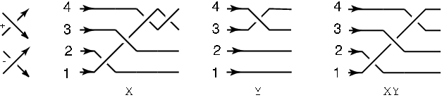
Pictures like the ones in Figure 1 give an excellent intuitive feeling for the braid group, but one that quickly becomes complicated when one tries to pin down details. What is the ambient space? (It is a slice of 3-space.) Are admissible isotopies constrained to ? (Yes, we cannot allow isotopies in which the strands are allowed to loop over the initial points.) Does isotopy mean level-preserving isotopy? (No, it will not matter if we allow more general isotopies in , as long as strands don’t pass through one-another.) Are strands allowed to self-intersect? (No, to allow self-intersections would give the ‘homotopy braid group’, a proper homomorphic image of the group that is our primary focus.) Can we replace the ambient space by the product of a more general surface and an interval, for example a sphere and an interval? (Yes, it will become obvious shortly how to modify the definition.)
We will bypass these questions and other related ones by giving several more sophisticated definitions. In 1.1, 1.2 and 1.3 we will define the braid group and pure braid group in three distinct ways. We will give a proof that two of them yield the same group. References to the literature establish the isomorphism in the remaining case. In 1.4 we will demonstrate the universality of ‘braiding’ by describing four examples which show how braids have played a role in parts of mathematics which seem far away from knot theory.
1.1 and via configuration spaces
We define the topological concept of a braid and of a group of braids via the notion of a configuration space. This approach is nice because it gives, in a concise way, the appropriate equivalence relations and the group law, without any fuss.
The configuration space of points on the complex plane is:
A point on is denoted by a vector . The symmetric group acts freely on , permuting the coordinates in each . The orbit space of the action is and the orbit space projection is . Choosing a fixed base point , we define the pure braid group on strands and the braid group on strands to be the fundamental groups:
At first encounter doesn’t look as if it has much to do with braids as we illustrated them in Figure 1, but in fact there is a simple interpretation which reveals the intuitive picture. While the manifold has dimension , the fact that the points are pairwise distinct allows us to think of a point as a set of distinct points on . An element of is then represented by a loop which lifts uniquely to a path , where consists of coordinate functions satisfying if also , the base point. The graph of the simultaneous functions is a geometric (pure) braid. The appropriate equivalence relation on geometric braids is captured by simultaneous homotopy of the simultaneous paths, rel their endpoints, in the configuration space.
The group is the group which Artin set out to investigate in 1925 in his seminal paper [6] (however he defined it in a less concise way); in the course of his investigations he was led almost immediately to study . Indeed, the two braid groups are related in a very simple way. Let be the homomorphism on fundamental groups which is induced by the orbit space projection . Observe that the orbit space projection is a regular -sheeted covering space projection, with as the group of covering translations. From this is follows that the group is a subgroup of index in , and there is a short exact sequence:
| (1) |
1.2 and via generators and relations
We give two definitions of the group by generators and relations. The classical presentation for first appeared in [6]. We record it now, and will refer back to it many times later. It has generators and defining relations:
| (2) |
The elementary braid is depicted in sketch (i) of Figure 2.

Many years after Artin did his fundamental work, Birman, Ko and Lee discovered a new presentation, which enlarged the set of generators to a more symmetric set. Let , where . We define , and adopt the convention that whenever it is convenient to do so we will write the smaller subscript first. The new presentation has generators and defining relations:
| (3) | |||||
See sketch (ii) of Figure 2 for a picture of , and [23] for a proof that (2) and (3) define the same group. Both presentations will be needed in our work. Note that the new generators include the old ones as a proper subset, since for each
By (1) the pure braid group has index in . Let . (See sketch (iii) of Figure 2). The symmetry can be seen by tightening the strand at the expense of loosening the strand. It is proved in [6] and also in [65] that has a presentation with generators and defining relations:
| (4) | |||||
| (5) | |||||
| (6) | |||||
| (7) |
The relations in (4) come from the existence of a split short exact sequence, for every :
| (8) |
The map is defined by pulling out the last braid strand, and the image of under its inverse embeds in , as the subgroup generated by pure braids on the first strands. The free subgroup is generated by the braids . The pure braid group is infinite cyclic and generated by . Inducting on , the structure of via a sequence of semi-direct products is uncovered.
1.3 and as mapping class groups
Our announced goal in this review was to concentrate on areas where there have been new developments in recent years. While it has been known for a very long time that Artin’s braid group is naturally isomorphic to the mapping class group of an n-times punctured disc, people have asked us many times for a simple proof of this fact. We do not know of a simple one in the literature, therefore we present one here. In this case ‘simple’ does not mean intuitive and based upon first principles, rather it means using machinery which is normally available to a graduate student who has the tools learned in a first year graduate course in topology, and is preparing to begin research.
Let denote a 2-manifold of genus with boundary components and punctures, and let denote the groups of all orientation preserving diffeomorphisms of . Observe that we may assign the compact open topology to , making it into a topological group. The mapping class group of is , that is, the quotient of modulo its subgroup of all diffeomeorphisms of which are isotopic to the identity rel . We allow diffeomeorphisms in to permute the punctures, writing if they are to be fixed pointwise. Our interest in this article is mainly in the special case of .
Theorem 1
There are natural isomorphisms:
Proof: We begin with an intuitive description of how to pass from diffeomorphisms to geometric braids and back again. Choose any . While is in general not isotopic to the identity, its image in under the inclusion map is, because . Let denote the isotopy. If the punctures in are at then the paths defined by the traces of the points under the isotopy sweep out a braid in , and the equivalence class of this braid is the image of the mapping class in the braid group .
It’s a little bit harder to understand the inverse isomorphism, from the braid group to the mapping class group. One chooses a geometric braid and imagines it as being located in a slice of 3-space, with the bottom endpoints of the braid strands (which are oriented top to bottom) as being pinned to the distinguished points on the punctured disc. If one is very careful the braid strings can be laid down on the punctured disc so that they become non-intersecting simple arcs, each of which begins and ends at a base point. One then constructs a homeomorphism of the punctured disc to itself in such a way that the trace of the isotopy to the identity is the given set of non-intersecting simple arcs.
To prove the theorem, we begin by establishing the isomorphism between and . A good general reference for the underlying mathematics is Chapter 6 of the textbook [38]. As previously noted is a topological group. Also, is a closed subgroup of . The evaluation map is defined by . It is clear that is continuous with respect to the compact open topology on and the subspace topology for . The topological group acts -transitively on the disc in the sense that if are distinct points and are others then there is an such that . Observe that if then and if with , then are in the same left coset of in . In this situation it is shown in [127], part I, Sections 7.3 and 7.4, that the 3-tuple is a fiber space, with total space Diff, base space projection and fiber Diff. (It is a good exercise for a graduate student to prove this directly by constructing the required local product structure in an explicit manner.) The long exact sequence of homotopy groups of a fibration then gives the following exact sequence of groups and homomorphisms, where we focus on the range that is of interest:
The two end groups are trivial. The left middle group is and the right middle group is . The isomorphism of Theorem 1 is . Tracing through the mathematics one finds that in fact its inverse is the map that we described right after we stated the theorem. The assertion about is therefore true. The proof for can then be completed by comparing the short exact sequence (1), which says that is a finite extension of with quotient the symmetric group with a related short exact sequence for the mapping class groups:
| (9) |
1.4 Some examples where braiding appears in mathematics, unexpectedly
We discuss, briefly, a variety of examples, outside of knot theory, where ‘braiding’ is an essential aspect of a mathematical or physical problem.
1.4.1 Algebraic geometry
Configuration spaces and the braid group appear in a natural way in algebraic geometry. Consider the complex polynomial
of degree with distinct complex roots . The coefficients are the elementary symmetric polynomials in , and so we get a continuous map which takes roots to coefficients. Two points have the same image if and only if they differ by a permutation, so we get the same identification as in the quotient map , in quite a different way. Since we are requiring that our polynomial have distinct roots, a point is in the image of under the root-to-coefficient map if and only if the polynomial has distinct roots, i.e. if and only if its coefficients avoid the points where the discriminant
expressed as a polynomial in , vanishes. Thus can be interpreted as the complement in of the algebraic hypersurface defined by the equation , where is rewritten as a polynomial in the coefficients . (For example, the polynomial has distinct roots precisely when ). In this setting the base point is regarded as the choice of a complex polynomial of degree which has distinct roots, and an element in the braid group is a choice of a continuous deformation of that polynomial along a path on which two roots never coincide. There is a substantial literature in this area, from which we mention only one paper, by Gorin and Lin [84]. We chose it because it contains a description of the commutator subgroup of the braid group, and many people have asked the first author for a reference on that over the years. While there may be other references they are unknown to us.
1.4.2 Operator algebras
Our next example, taken from the work of Vaughan Jones [87],[88], is interesting because it shows how ‘braiding’ can appear in disguise, so that initially one misses the connection. We consider the theory, in operator algebras, of ‘type II1 factors’, ordered by inclusion. Let denote a Von Neumann algebra, i.e. an algebra of bounded operators acting on a Hilbert space . The algebra is called a factor if its center consists only of scalar multiples of the identity. The factor is type II1 if it admits a linear functional, called a trace, , which satisfies the following three conditions: (i) , (ii) , and , where is the adjoint of . In this situation it is known that the trace is unique, in the sense that it is the only linear functional satisfying the first two conditions. An old discovery of Murray and Von Neumann was that factors of type II1 provide a type of ‘scale’ by which one can measure the dimension of . The notion of dimension which occurs here generalizes the familiar notion of integer-valued dimensions, because for appropriate and it can be any non-negative real number or .
The starting point of Jones’ work was the following question: if is a type II1 factor and if is a subfactor, is there any restriction on the real numbers which occur as the ratio ? The question has the flavor of questions one studies in Galois theory. On the face of it, there was no reason to think that could not take on any value in , so Jones’ answer came as a complete surprise. He called the index of in , and proved a type of rigidity theorem about type II1 factors and their subfactors:
The Jones Index Theorem: , where . Moreover, each real number in the continuous part of the spectrum and in the discrete part is realized.
What does all this have to do with braids? To answer the question, we sketch the idea of the proof, which is to be found in [87]. Jones begins with the type II1 factor and the subfactor . There is also a tiny bit of additional structure: It turns out that in this setting there exists a map , known as the conditional expectation of on . The map is a projection, i.e. . His first step is to prove that the ratio is independent of the choice of the Hilbert space . This allows him to choose an appropriate so that the algebra generated by and makes sense. He then investigates and proves that it is another type II1 factor, which contains as a subfactor, moreover . Having in hand another II1 factor and its subfactor , there is also a trace on (which by the uniqueness of the trace) coincides with the trace on when it is restricted to , and another conditional expectation . This allows Jones to iterate the construction, to build algebras and from them a family of algebras , where is generated by .
Rewriting history a little bit in order to make the subsequent connection with braids a little more transparent, we now replace the projections , which are not units, by a new set of generators which are units, defining: , where . The ’s generate because the ’s do, and we can solve for the ’s in terms of the ’s. So is generated by and we have a tower of algebras, , ordered by inclusion. The parameter , which replaces the index , is the quantity now under investigation. It’s woven into the construction of the tower. The algebra has defining relations:
| (10) | |||
Of course there are braids lurking in the background. If we rename the , replacing by , and declare the to be generators of a group, then the first two relations are defining relations in the group algebra . The algebra is thus a homomorphic image of the group algebra of the braid group. Loosely speaking, braids are encountered in Operator Algebras because they encode the way in which each type II1 factor acts on its subfactor . Braiding is thus involved in defining the associated extensions. We shall see later, in 4.7 that a similar action, via group extensions, can be used to define representations of .
To see the connection with knots and links, recall that since is type II1 it supports a unique trace, and since is a subalgebra it does too, by restriction. This trace is known as a Markov trace, i.e. it satisfies the important property:
| (11) |
where is a fixed function of . Thus, for each fixed value of the trace is multiplied by a fixed scalar when one passes from one stage of the tower to the next, if one does so by multiplying an arbitrary element of by the new generator of . The Jones trace is nothing more or less than the 1-variable Jones polynomial [89] associated to the knot or link which is obtained from the closed braid. We will have more to say about all this in 4.3.
1.4.3 Homotopy groups of spheres
As before, let denote the pure braid group on strands. For each there is a natural homomorphism , defined by pulling out the strand. The group of Brunnian braids is
i.e. a braid is in if and only if, on pulling out any strand, it becomes the identity braid on strands. Brunnian braids have received some attention in knot theory.
Braids have played a role in homotopy theory for many years, most particularly in the work of F. Cohen and his students (see for example [10]), but during the past few years the connection was sharpened when it was discovered that there is an embedding of a free group in with the property that a well-defined quotient of (a little bit too complicated to describe here) is isomorphic to . It remains to be seen whether new knowledge about the unidentified higher homotopy groups of spheres can be obtained through the methods of [10].
1.4.4 Robotics
Our fourth example is an application of configuration spaces to robotics. It shows the braid group popping up in an unexpected way (until you realize how natural it is). Robots, or AGVs (automatic guided vehicles), are required to travel across a factory floor that contains many obstacles, en route to a goal position (e.g. a loading dock or an assembly workstation). The problem is to design a control system which insures that the AGVs not collide with the obstacles, or with each other, and complete the task with efficiency with regard to various work functionals. Here is how configuration spaces appear: The underlying space in this simple example is the workspace floor , from which a finite set of obstacles are to be removed. The configuration space of non-colliding AGVs is then precisely . More generally, is replaced by a finite graph , and the the braid group by the braid group of the graph. There is a vast literature on this subject; we suggest [78] by R. Ghrist, as a starter.
1.4.5 Public key cryptography
In this example braids are important for rather different reasons than they were in our earlier examples. In our earlier examples the underlying phenomenon which was being investigated involved actual braiding, albeit sometimes in a concealed way. In the example that we now describe particular properties of the braid groups , rather than the actual interweaving of braid strands, are used in a clever way to construct a new method for encrypting data.
The problem which is the focus of ‘public key cryptography’ will be familiar to everyone: the security of our online communications, for example our credit card purchases, our ATM transactions, our cell phone conversations and a host of other transactions that have become a part of everyday life in the century, The basic problem is to encrypte or translate a secret message into a code that can be sent safely over a public system such as the internet, and decoded at the receiving end by the use of a secret piece of information known only to the sender and the recipient, the ‘key’. The problem that must then be solved is to establish a private key that will be known only to the sender and the recipient, who will then be able to exchange information over an insecure channel. In recent years much work has been done on certain codes which are based upon the assumption that the word problem has polynomial growth as braid index is increased, whereas the conjugacy problem does not. But in 5 we will review recent work on the word and conjugacy problems in the braid groups, and show that such an assumption seems problematic at best. See 5, and in particular the discussion in 5.5 below.
Acknowledgements: We thank Tahl Nowik, who suggested, during a course that the first author gave on mapping class groups, that techniques she had used for other purposes could be adapted to give the proof we presented here of Theorem 1. We also thank Robert Bell, David Bessis, Nathan Broaddus, John Cannon, Ruth Charney, Fred Cohen, Patrick Dehornoy, Roger Fenn, Daan Krammer, Lee Mosher, Luis Paris, Richard Stanley, Morwen Thistlethwaite and Bert Wiest for their help in chasing down facts and references, and helping us fill gaps in our knowledge. We would particularly like to thank all the students who attended Math 661 in the Fall of 2003 at Cornell University, who were gracious guinea pigs for large parts of this article, especially Heather Armstrong, whose careful attention and diligence significantly improved the manuscript, and Bryant Adams, who suggested the proof of Lemma 2.2 to us.
2 From knots to braids
In this chapter we will explore, for the benefit of readers who are new to the subject, the foundations of the close relationship between knots and braids. We will first describe the straightforward process of obtaining a knot or a link from a given braid by ‘closing’ the braid. This leads us directly to formulate two fundamental questions about knots and braids. First, is it always possible to transform a given knot into a closed braid? This question will be answered in the affirmative in Theorem 2, first proved by Alexander in 1928 in [2]. The correspondence between knots and braids is clearly not one-to-one (for example, conjugate braids yield equivalent knots), leading naturally to the second question: which closed braids represent the same knot type? That question is addressed in Theorem 4, first formulated by A. Markov in [104], which gives ‘moves’ relating any two closed braid representatives of a knot or link, while simultaneously preserving the closed braid structure.
Together, Theorems 2 and 4 form the cornerstone of any study of knots via closed braids, so we feel obliged to prove them. Among the many proofs that have been published of both over the years, we have chosen ones that we like but which do not seem to have appeared in any of the review articles that we know. The proof that we give of Alexander’s Theorem is due to Shuji Yamada [136], with subsequent improvements by Pierre Vogel [135]. The algorithm is elementary enough to be accessible to a beginner, and has the advantage for experts of being suitable for programming. The proof that we present of Markov’s theorem is due to Pawel Traczyk [129]. It is relatively brief, as it assumes Reidemeister’s well-known theorem about the equivalence relation on any two diagrams of a knot, Theorem 3 below, building on methods introduced in the proof of Theorem 2.
2.1 Closed braids
For simplicity, let us begin with a planar diagram of a given geometric braid. To obtain a knot or link, one simply ‘closes up’ the ends of the braid as in Figure 3.

The pre-image in of the ‘center point’ shown in Figure 3 under the usual projection map is called the axis of the braid. (If one wishes to consider the knot in , then we include the point at infinity so that the braid axis is an embedded .) We then orient the resulting knot or link in such a way that the strands of the braid are all travelling counterclockwise about the braid axis. The knot or link type resulting from performing this operation on a braid is known as the closure of and will be denoted by . The same notation may also refer to the particular diagram as in Figure 3.
Equivalently, consider a knot . Suppose there exists where is an embedding and is unknotted in and contained in the complement of . Suppose further that we choose the point at infinity to be in and, using standard cylindrical coordinates on , identify the resulting copy of with the -axis in . If we always have as we travel about the knot with an appropriate cylindrical parametrization, then we say that is a closed braid with respect to the axis . The closed braid diagram of Figure 3 is then obtained by projection parallel to the direction defined by onto a plane that is orthogonal to .
2.2 Alexander’s Theorem
As we just observed, it is a simple matter to obtain a knot or link from a braid. The classical theorem of J. Alexander allows us to reverse this process, though not in a unique way:
Theorem 2
(Alexander’s Theorem [2]) Every knot or link in can be represented as a closed braid.
Proof: Alexander’s original proof was algorithmic, i.e. it gave an algorithm for transforming a knot or link into closed braid form. While it is straightforward, we do not know of any computer program based upon it. We shall give instead a rather different and newer algorithm originally due to Yamada [136], as later improved by Vogel [135]. We like it for two reasons: (1) It has a beautiful corollary (see Corollary 2.1 below) which reveals structure about knot diagrams that had not even been conjectured by any of the experts before 1987, even though there was abundant evidence of its truth; (2) It leads, very easily, to an efficient computer program for putting knots into braid form. In this regard we note that when Jones was writing the manuscript [88], which resulted in his award of the Fields medal, he computed closed braid representatives for the 249 knots of crossing number less than or equal to 10, constructing the first table known to us of closed braid representatives of knots. His list remains extremely useful to the workers in the area in 2004. Yamada’s work was not yet known when he did that work, and there did not seem to him to be a good way to program the Alexander method for a computer, so he calculated them one at a time by hand. The amount of work that was involved can only be appreciated by the reader who is willing to try a few examples.
In order to prove Alexander’s Theorem, we shall first present the Yamada-Vogel algorithm for transforming a knot into closed braid form in full, followed immediately by an illustrative example (Example 2.1). We shall then prove Alexander’s Theorem by showing that it is always possible to perform the steps of the Yamada-Vogel algorithm for any given knot or link and that the algorithm always leads to a closed braid.
The Yamada-Vogel algorithm draws on Seifert’s well-known algorithm for using a diagram of an oriented knot or link to construct a Seifert surface for (see [123] or [101], e.g., for a thorough treatment of Seifert’s algorithm), and we will need some related terminology. Let and be two oriented disjoint simple closed curves in . Then and cobound an annulus . We say that and are coherent (or coherently oriented) if and represent the same element of . Otherwise we say that and are incoherent. Following Traczyk [129], we define the height of a knot diagram , denoted , to be the number of distinct pairs of incoherently oriented Seifert circles which arise from applying Seifert’s algorithm to . The height function gives us a useful characterization of a closed braid: a diagram represents a closed braid if and only if . (Recall that lives in .)
The Yamada-Vogel Algorithm
- 1.
Let be a diagram of an oriented knot . Smooth all crossings of as in Seifert’s algorithm to obtain Seifert circles . Record each original crossing with a signed arc: for a positive crossing (often called a right-handed crossing), for a negative (or left-handed) crossing (see Figure 2(iv)). The resulting diagram is the Seifert picture corresponding to the diagram . Note that any two circles joined by a signed arc in any Seifert picture are necessarily coherent. For an example that illustrates the construction of a Seifert diagram, see the passage from the bottom left to the top left sketches in Figure 4.
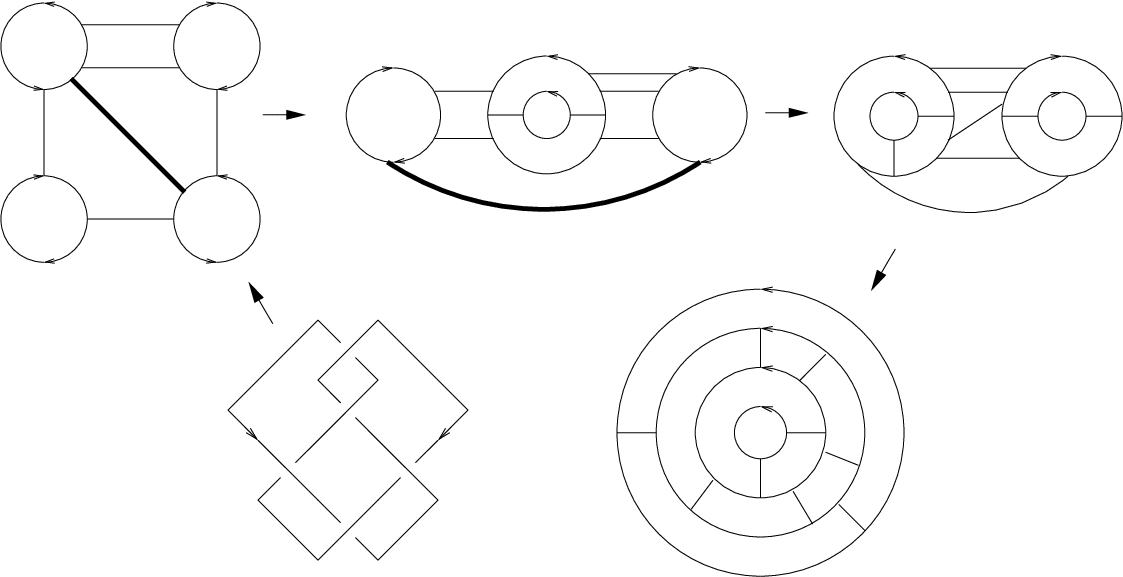
Figure 4: The Yamada-Vogel algorithm performed on the knot . - 2.
If , the knot is already in closed braid form, and we are done. If , we can find a reducing arc , i.e., an arc joining an incoherent pair such that intersects only at its endpoints. Reducing arcs are illustrated as heavy black arcs in the example in Figure 4. A component of which admits a reducing arc is called a defect region. Perform a reducing move along , as shown in Figure 5, to obtain a new Seifert picture in which a pair of coherent Seifert circles, and , joined by two oppositely signed arcs, replaces the incoherent pair . The corresponding move on the original diagram is a Reidemeister move of type II in which we slide over in a small neighborhood of the arc to obtain a new diagram with two new crossings. Note that if we instead slide under , we obtain the same two new Seifert circles but the signs of the two new signed arcs are now switched.

Figure 5: The local picture of a reducing move. - 3.
Continue performing reducing moves on incoherent pairs until a diagram with height zero is obtained.
Example 2.1
We apply the Yamada-Vogel algorithm to the diagram of the knot , pictured in Figure 4. (The reader can check that this is the first example in the knot tables of a knot diagram with height greater than zero.) The first stage shows the Seifert picture associated to the original diagram, consisting of 4 Seifert circles, with 5 signed arcs (all positive) recording the original crossings. We see that the original knot diagram has height 2. The figure shows a choice of reducing arc, , joining one of the two pairs of incoherent circles.
In the third sketch of Figure 4, we see the new Seifert picture resulting from performing the reducing move along . Note that we have introduced two new crossings of opposite sign. We also see a new reducing arc, , joining the only remaining pair of incoherent circles. We see in the fourth sketch the Seifert picture with height zero resulting from the second reducing move performed along . At this point, we are done, but in the final sketch we see a different planar projection of the same Seifert picture which allows us easily to read off a braid word associated to the knot: beginning with the positive signed arc in the ‘twelve o’clock’ position and reading counter-clockwise, we see that the knot is equivalent to , where .
We may learn several things from this simple example. Applying the braid relations to the word defined by , we see that Since this braid only involves once, we may ‘delete a trivial loop to get the 8-crossing 3-braid so the algorithm did not give us minimum braid index. The algorithm also does not give shortest words because our 8-crossing braid may be shortened to the 6-crossing 3-braid In fact, 6 is minimal, because the crossing number of a 3-braid knot must be even, and this knot has no diagram with fewer than 5 crossings, so 6 is minimal. So we may deduce one more fact: when we use the Yamada-Vogel algorithm to change a knot which is not in closed braid form to one which is, the crossing number goes up.
To prove Alexander’s Theorem, we first need to show that a reducing move strictly decreases the height of a diagram. This lemma is sometimes stated as ‘obvious’ in the literature, but the question arises frequently enough to warrant a short but thorough argument.
Lemma 2.1
Suppose a reducing move is performed which transforms a diagram to a diagram . Then .
Proof. Let be the Seifert circles in the Seifert picture corresponding to the diagram . Let be an incoherent pair. The union separates the 2-sphere into three components: an annulus cobounded by and , and two disks, and bounded by and , respectively. Suppose that admits a reducing arc . A reducing move along preserves circles and replaces and with two new circles, one of which necessarily bounds a disk containing no other Seifert circles in the new Seifert picture . We denote this circle by (see Figure 5). The other new circle, denoted , bounds a disk containing all Seifert circles originally contained in the annulus in .
To simplify the bookkeeping, we shall write if the pair is coherent, or else if are incoherent. Obviously, if , then is unchanged by the reducing move, so we need only consider the effect of the reducing move on , where or and . Now if is contained in the annulus in (and hence in in ), then clearly . Also, if in , then and . Similarly, if in , then and . Therefore the number of distinct incoherent pairs in with is equal to the total number of distinct incoherent pairs in of the form with . By construction, however, we have replaced with . Thus .
The previous lemma tells us that the Yamada-Vogel algorithm will always lead to a diagram of height zero, i.e., a closed braid, as long as it is always possible to perform Step 3. Therefore the following lemma, whose proof was suggested to us by Bryant Adams, will conclude the proof of Alexander’s Theorem.
Lemma 2.2
[136] Let be a knot or link diagram. If , then the Seifert picture associated to contains a defect region.
Proof: Each component of is a surface of genus with boundary components. Each boundary component of is a union of some number of signed arcs (possibly zero) and subarcs of Seifert circles. We call the collection of Seifert circles in which form part or all of a boundary component of the exposed circles of .
Let us now examine the possible ways in which could fail to be a defect region. Certainly, if has one exposed circle, then it is not a defect region. If has two exposed circles, then is either a disk or an annulus. In this case, if is a disk, then its two exposed circles are joined by at least one signed arc; hence the two circles are coherent and is not a defect region. If is an annulus, either its two exposed circles are incoherent, in which case it is a defect region, or else they are coherent and is not a defect region. If has three or more exposed circles, then there is necessarily one incoherent pair among them, and is a defect region.
Suppose that no component of is a defect region and hence that each component is of one of the three types of non-defect regions described above. It is clear that we must have at least one region of the second type, since otherwise is clearly zero. We can think of such a region as lying between two nested, coherent circles joined by at least one signed arc.
Let us now start with such a region, and try to build a diagram with no defect regions. We cannot add any circles in the annulus cobounded by the two nested circles, since this necessarily gives rise to at least one component with three or more exposed circles. In fact, our only option is to add coherent circles which nest with the original two circles (and as many signed arcs between adjacent pairs as we like). However, such a diagram has height zero. Therefore, implies that a defect region exists. This completes the proof of Lemma 2.1, and so also of Theorem 2.
The braid index of a knot or link is the minimum number such that there exists a braid whose closure represents . (We note that it is also common to refer to the index of a braid or a closed braid, meaning simply the number of its strands or the number of times it travels around its axis, respectively.) It is clear that the minimum number of Seifert circles in any diagram of a knot or link is bounded above by the braid index of . It is equally clear from the Yamada-Vogel algorithm that the reverse inequality holds. Thus we obtain the following corollary, which is due to Yamada [136]. It seems remarkable that it was not noticed long before 1987.
Corollary 2.1
[136] The minimum number of Seifert circles in any diagram of a knot or link is equal to the braid index of .
It also follows that we have a measure of the complexity of the process of transforming a knot into closed braid form as follows.
Corollary 2.2
([129], [135]) Let denote the length of any sequence of reducing moves required to transform a diagram into closed braid form. Then we have:
| (12) |
where is the number of Seifert circles associated to .
Open Problem 1
It is an open problem to determine, among all regular diagrams for a given knot or link, the minimum number of Seifert circles that are needed. By Corollary 2.1 this is the same as the minimum braid index, among all closed braid representatives of a given knot or link. We know of only one general result relating to this problem, namely the Morton-Franks-Williams inequality of [111] and [74]. It will be discussed briefly in 4.3. The literature also contains an assorted collection of ad-hoc techniques for determining the braid index of individual knots. For example, see the methods used in [31] to prove that the 6-braid template in Figure 20 below actually has braid index 6, which rests on the fact that non-trivial braid-preserving flypes always have braid index at least 3.
2.3 Markov’s Theorem
To introduce the main goal of this section, we begin by recalling for the reader Reidemeister’s theorem, which dates from the earliest days of knot theory. It was assumed and used (as a folk theorem) long before anybody wrote down a formal statement and proof.
Theorem 3
(Reidemeister’s Theorem) Let be any two (in general not closed braid) diagrams of the same knot or link . Then there exists a sequence of diagrams such that any in the sequence is obtained from by one of the three Reidemeister moves, depicted in Figure 6.

Proof: We refer the reader to [43] for a complete proof.
Alexander’s Theorem, proved in the last section, guarantees us that closed braid representatives of a knot exist, but as previously noted, they are certainly not unique. Markov’s Theorem, first stated in [104] with a sketch of a proof, gives us a certain amount of control over different closed braid representatives of the same knot. It asserts that any two are related by a finite sequence of elementary moves and serves as the analogue for closed braids of the Reidemeister Theorem for knots.
One of the moves of the Markov Theorem is braid isotopy. From the point of view of a topologist, braid isotopy means isotopy of the closed braid, through braids, in the complement of the braid axis. Morton has proved that if two braids have closures that are braid isotopic, then they are conjugate in [108]. The other two moves that we need are mutually inverse, and are illustrated in Figure 7 as a move on certain -braids. We call them destabilization and stabilization, where the former decreases braid index by one and the latter increases it by one. The weight that is attached to one of the braid strands in Figure 7 denotes that many ‘parallel’ strands, where parallel means in the framing defined by the given projection. The braid inside the box which is labelled P is an arbitrary -braid. Later, it will be necessary to distinguish between positive and negative destabilizations, so we illustrate both now.

Theorem 4
(Markov’s Theorem) Let be closed braid representatives of the same oriented link type in oriented 3-space. Then there exists a sequence of closed braid representatives of :
taking such that each is obtained from by either (i) braid isotopy, or (ii) a single stabilization or destabilization.
We call the moves of Theorem 4 Markov moves, and say that closed braids that are related by a sequence of Markov moves are Markov-equivalent.
Forty years after Markov’s theorem was announced, the first detailed proof was published in [18]. At least 5 essentially different proofs exist today. See for example [110], in which Morton gives his beautiful threading construction for knots and braids which also yields an alternate proof of Alexander’s Theorem. Here we shall present a proof due to Pawel Traczyk [129]. It begins with Reidemeister’s theorem, and uses the circle of ideas that were described in the previous section, and so it is particularly appropriate for us.
Proof: We are given closed braids which represent the same oriented knot type . Without loss of generality we may assume that and are defined by closed braid diagrams of height . By Theorem 3 we know there is a sequence of knot diagrams , where in general for , such that any two diagrams in the sequence are related by a single Reidemeister move of type I, II or III. The first step in Traczyk’s proof is to reduce the proof to sequences of knot diagrams which are related by Yamada-Vogel reducing moves:
Lemma 2.3
It suffices to prove Theorem 4 for closed braid diagrams which are related by sequences with the properties (i) , (ii) for , and (iii) is obtained from by a single Yamada-Vogel reducing move or the inverse of a reducing move.
Proof: We may always assume that the diagrams have height , for if not we simply replace the given sequences by the subsequences joining any two intermediate diagrams of height zero.
We say that a Reidemeister move is braid-like if the strands that are involved in it are locally oriented in a coherent fashion, as they would be if the diagram is a closed braid. In particular, any Reidemeister move of type I is braid-like. To begin the proof of the lemma, we establish a somewhat weaker result: we claim that we can get from to via a finite sequence of the following four types of moves and their inverses:
a braid-like Reidemeister move of type I, denoted type Ib,
a braid-like Reidemeister move of type II, denoted type IIb,
a braid-like Reidemeister move of type III, denoted type IIIb,
a Yamada-Vogel reducing move, denoted type .
To prove the claim, it is enough to show that non-braid-like Reidemeister moves, which we denote by the symbols Inb, IInb and IIInb, can be achieved via a finite sequence of moves of type Ib, IIb, IIIb and . To prove this, we examine the cases Inb, IIInb and IInb in that order:
- 1.
As previously noted, any type I Reidemeister move is of type Ib.
- 2.
A type IIInb Reidemeister move involves three arcs of the knot or braid. There are many different cases, depending on the local orientations and the signs of the 3 crossings, but they are all similar. One of the possible cases is given by the first and last sketches of Figure 8, where an arc passing under a crossing formed by the other two arcs is locally oriented opposite to the other two strands. The replacement sequence that is given in Figure 8 shows that our type IIInb Reidemeister move can be achieved by a sequence consisting of a type IInb move, an isotopy, a type IIIb move and finally another type IInb move. We leave the other type IIInb cases to the reader, and we have reduced to the case of moves of type IInb.

Figure 8: Replacing moves of type IIInb - 3.
A move of type IInb may be regarded as a move of type if the arcs that are involved belong to distinct Seifert circles, so we only need to handle the case where they are subarcs of the same Seifert circle. This is done in Figure 9, where it is shown that the move can be replaced by two moves of type Ib (which create two new Seifert circles) followed by a move of type and another of type . This proves the claim.
 |
We are thus reduced to the case in which each diagram in the sequence taking to is either type Ib, IIb, IIIb or . To complete the proof of Lemma 2.3, let be a braid-like Reidemeister move to be performed on diagram . Suppose that . Then we can find a sequence of reducing moves such that is a braid and such that the associated reducing arcs are each disjoint from the region in which is to be performed. Thus each reducing move commutes with , and we can replace with its ‘conjugate’ , so that is now performed at height , i.e., on a braid.
If is of type IIb or IIIb, then we are done, since a braid-like move of type II or type III performed on a braid is a braid isotopy. If is of type Ib, it is a stabilization (up to isotopy) only if it is performed on the braid strand ‘nearest’ to the braid axis. However, it is not hard to see how to realize a type Ib move on an arbitrary strand in terms of Markov moves: simply push the strand under the others via type IIb moves, and perform the required stabilization in a neighborhood of the braid axis. Note that to pass the resulting ‘kink’ back under a neighboring strand in a braid requires first a type IIIb move followed by a type move (the ‘kink’ is always its own Seifert circles, so two distinct circles are necessarily involved). Thus we can return the strand with the ‘kink’ in it back to its original position by repeated applications of this two-step process. Since we have just seen that any type IIb or type IIIb move can be realized by a finite sequence of type moves and braid isotopies, this means that a type Ib move can also be replaced by a finite sequence of type moves and braid isotopies. We can handle inverse moves of type Ib in a similar fashion
We have thus replaced our original sequence relating to by a new one which is in general much longer, but which consists entirely of Markov moves (performed, by definition, on braid diagrams, i.e., on diagrams of height zero) and moves of type . To be precise, our original sequence from to may be replaced by a sequence of the form , where for all and in each subsequence , either (1) each diagram in the subsequence has height zero and adjacent diagrams are related by a single Markov move, or (2) all the intermediate diagrams have strictly positive height and adjacent diagrams are related by a single move of type or . Therefore in order to prove Markov’s theorem, it suffices to consider only sequences of the second type, and the proof of Lemma 2.3 is complete.
Remark 2.1
The astute reader will have noticed the following: we have eliminated Reidemeister moves completely (they will not appear in the arguments that follow), nevertheless they played an important role already. We started with a sequence relating the given braids and that consisted entirely of Reidemeister moves. We replaced it with a sequence of reducing moves and braid-like Reidemeister moves. The latter are in general not applied to diagrams of height zero, but we changed them to apply to diagrams of height zero. That is the moment when Traczyk’s braid-like Reidemeister moves were changed to Markov moves. The modified sequence from to has changed to a series of subsequences, each of which starts with a closed braid and ends with a closed braid, after which the ending braid is modified (by Markov moves) to a new closed braid, which is the initial closed braid in the next subsequence. As will be seen, Markov moves will not be used explicitly again until the proof of Lemma 2.8, where they are used (without the help of Reidemeister’s Theorem) to relate very special closed braid diagrams.
Consider now a sequence of diagrams satisfying the criteria of Lemma 2.3. We note that, as in the above proof, we shall not in general distinguish between a diagram and its associated Seifert picture. Thus we shall make reference to ‘a Seifert circle in the diagram ’, for example, meaning a Seifert circle in the Seifert picture associated to . In fact, we can think of each circle in a Seifert picture as forming part of the associated diagram, except in a small neighborhood of signed arcs, which correspond to crossings. Since reducing arcs avoid signed arcs, there is no ambiguity when referring to ‘a reducing arc in a diagram’.
We now wish to consider the graph of the height function on our sequence. The graph will begin and end at height zero; each ‘step’ in between will either take us up 1 or down 1 since we have reduced to the case where all moves are reducing moves (or their inverses). We will examine local maxima in the height function. Let be three consecutive diagrams in our sequence such that the height function has a local maximum at . In other words, we have two reducing moves with corresponding arcs in such that reducing along (resp. ) results in the diagram (resp. ), and it makes sense discuss . We will call such a triple a peak in the height function of our sequence. We define the height of the peak to be and define the height of the sequence to be the maximum value attained by the height function on the sequence, in other words, the maximum over the height of all the peaks in the sequence. In order to prove Theorem 4, we are going to induct on the height of the sequence.
Lemma 2.4
We may assume that the reducing arcs involved in any peak in the height function of our sequence are disjoint. Further, the adjustments in our sequence of reducing moves which are required preserve the height of the sequence.
Proof: Let be a peak in the height function with associated reducing arcs and . We may always assume that the arcs intersect transversally and minimally. Suppose that . By smoothing out one or more of the points of intersection, we find a new reducing arc with the same endpoints as such that and . We can then replace the given peak with two consecutive peaks and . We call this procedure inserting the reducing operation at , and it essentially amounts to replacing one peak with two peaks of the same height. In this way, we continue on until the intersection numbers of all adjacent pairs is at most .
Now suppose the arcs associated to a given peak have intersection number . If there exists a reducing arc such that , then we can insert the reducing operation at to produce two peaks, each with a disjoint pair of associated reducing arcs. Suppose that the defect region which supports and contains no third reducing arc which is disjoint from both and . There is only one possible arrangement for such a defect region, shown in Figure 10.

With this arrangement, the reducing arcs and must act on four distinct Seifert circles, possibly joined by signed arcs. We will now examine the region labelled which lies ‘outside’ of the circles involved in our defect region and the signed arcs which join them. If contains a Seifert circle, then it is easy to check that there must be a region somewhere in the diagram with three exposed circle. Such a region, as observed in the previous section, is necessarily a defect region which would contain a reducing arc disjoint from both and . If, on the other hand, contains no Seifert circles, then it contains no signed arcs either, since all possible signed arcs between the four exposed circles of region already appear in Figure 10. Thus we can join either pair of diagonally opposed circles by a reducing arc in .
We conclude that if a peak has associated arcs of intersection 1, we can always find a third reducing arc so that we can insert the reducing operation at , thereby replacing the original peak with two peaks, each having a disjoint pair of reducing arcs. Since the operation of inserting a reducing operation at a peak preserves the height of the sequence, this finishes the proof of the lemma.
Thanks to the previous lemma, we can assume from now on that each peak in the graph of our height function corresponds to a disjoint pair of reducing arcs. Before we can state the next lemma, which concerns the peaks in the height function, we need to introduce a few some concepts. Note that when the reducing arcs involved in a peak are disjoint, the reducing moves commute, that is, they can be performed in either order, starting with the diagram and resulting in the same diagram . Further, as long as the reducing arcs act on 3 or 4 distinct Seifert circles, we can perform the two reducing moves in either order with the same result. Observe that, since the reducing arcs are disjoint in the diagram , it makes sense to talk about the arc (resp. ) in the context of the diagram (resp. ) obtained by reducing along (resp. ). In this case we say we have a ‘commuting pair’ of reducing moves associated to the peak. If a peak has a commuting pair, then we may replace it by a ‘valley’, that is, a subsequence where and is the result of reducing along , or equivalently reducing along . Thus we can eliminate any peak corresponding to a commuting pair (such a peak necessarily has height at least 2).
In the case where two reducing arcs at a peak act on the same 2 circles, then after one move is performed, the second Reidemeister move will no longer be a reducing move; we call this a ‘non-commuting pair’ of reducing moves. Let be a peak corresponding to a non-commuting pair of reducing arcs, and let be the two Seifert circles involved. Suppose there is a reducing arc such that and such that involves a circle other than or , then we can insert at to replace our peak with two new peaks with commuting pairs of reducing moves: and . As above, we now replace each peak with a ‘valley’: and , respectively, where is the diagram resulting from reducing by (or equivalently, from reducing by , and is the diagram resulting from reducing by (or equivalently, from reducing by ). Again, this implies that the height of the original non-commuting peak was at least 2. Thus, we can replace such a peak with peaks of strictly smaller height and repeat this process until all peaks either have height 1 or do not admit such a reducing arc as above; we call a peak of the latter type irreducible.
We can now state the next lemma:
Lemma 2.5
We may assume that any peak in the height function of our sequence either has height 1 or is irreducible.
Proof: The proof is clear. In the discussion that preceded the statement of the Lemma we defined a peak to be irreducible in such a way that it subsumed all possibilities which did not allow us to reduce to height 1.
We note that each condition of Lemma 2.5 necessarily implies the non-commuting condition.
Lemma 2.6
We may assume that no peaks in the height function of our sequence have height 1.
Proof: Let be a peak of height 1. We recall that height 1 implies that the two reducing arcs are non-commutative and hence involve precisely two circles. it is an easy exercise to show that these two circles must live either on the ‘inside’ or on the ‘outside’ of a band of circles, and that and are in fact equivalent as reducing moves. Therefore the diagram is equivalent to and we can simply eliminate this peak from our sequence.
It remains to deal with irreducible peaks in the height function of our sequence. Fortunately, it turns out that they only occur in a very particular way. To describe the particular way, define a weighted Seifert circle in a manner which is similar to the weights that we attach to closed braid diagrams, e.g. as in Figure 7. That is, A Seifert circle with weight attached means a collection of coherently oriented, nested, parallel Seifert circles. We use the term band for a Seifert circle with an attached weight.
Lemma 2.7
If is an irreducible peak in the height function of our sequence, then the diagram contains at most four bands, arranged as in Figure 11.
Proof: Let be an irreducible peak, and let be the two circles involved in the reducing arcs and . See Figure 11(i).

For , let denote the disk bounded by in which does not contain the reducing arcs and . Then has two components. By assumption, neither component can contain a defect region (or else we could find a reducing arc as above, contradicting the irreducibility of our peak). Thus if either component contains any Seifert circles, the circles must form a band, oriented oppositely to and . We allow the possibility that the weight of these bands is zero. The same reasoning shows that cannot contain a defect region for and hence that must be the outer circle of a band. It is of course possible that some braiding takes place between adjacent coherent circles, as indicated in Figure 11(i). The braids joining the various bands are labelled . Thus we have a diagram of the given form, in which each circle pictured represents a band, and the lemma is proved.
The following lemma will allows us to replace irreducible peaks in the height function of our sequence with peaks of strictly smaller height.
Lemma 2.8
Let be an irreducible peak of height in the height function of our sequence. Then there exist sequences of diagrams and such that (resp. ) is obtained from (resp. ) by a reducing move and such that and and are Markov equivalent.
Before discussing the proof of this lemma, we show how to use it to prove the Markov theorem. Using Lemmas 2.3-2.7, we have reduced the proof of Markov’s Theorem to the situation of two closed braid diagrams and related by a sequence of diagrams related by reducing moves (and their inverses) such that the height of each intermediate diagram is strictly positive and such that any peak in the height function of the sequence is irreducible (of height at least 2). Let be an irreducible peak of height in the height function of our sequence. By Lemma 2.8, we can replace this subsequence with a subsequence of strictly smaller height (possibly including a subsequence entirely at height 0 related by Markov moves, which we can remove from consideration as before). In doing so, we create new peaks whose height is strictly lower than the height of the peak being replaced. If we perform this operation at every irreducible peak, then we obtain a new sequence relating our closed braid diagrams .
The new peaks may or may not be irreducible; in fact, their corresponding arcs may not even be disjoint, but now we are back in the same situation as we were before Lemma 2.4 except that we are starting with a sequence of lower height. Thus by induction on the height of the sequence (with base case provided by Lemma 2.6), we can replace any sequence as described in Lemma 2.3 with a sequence consisting entirely of diagrams of height zero. This completes the proof of Theorem 4, modulo the proof of Lemma 2.8.
Sketch of the Proof of Lemma 2.8. By Lemma 2.7, the diagram has at most four bands which we label , and , joined by four (possibly trivial) braids , as in Figure 11(i) and (ii). Let denote the weight of the band . Note that, e.g., the braid has strands, and similarly for the other . If or is greater than 1, then a reducing arc joining is understood to indicate a sequence of reducing moves. There are several ways to construct such a sequence; we adopt the convention that we choose reducing moves in such a way that the strands of one band all slide under or else all slide over the strands of the other band.
Referring again to Figure 11, we first perform the reducing move along the arc and then reduce again via the arc involving and , giving us some number of reducing moves depending on the weights of the bands involved. The resulting diagram is the closure of the first braid shown in Figure 12, up to a choice of arcs passing over or under in the various Reidemeister moves of type II. This gives us the first sequence of the lemma.

To get the second sequence of the lemma, we begin instead with the reducing move along the arc and then reduce again via the arc . The resulting diagram is the closure of the second braid shown in Figure 12.
We have found our two sequences of reducing moves, and we have reduced the proof of Markov’s Theorem to just one specific calculation, namely, showing that the closed braids and corresponding to the two braids of Figure 12 are M-equivalent. The two braids can be related by a sequence consisting of several braid isotopies as well as two stabilizations and two destabilizations; the reader is referred to [129] for the details of this calculation. This concludes the proof of Lemma 2.8, and so also of Theorem 4.
Remark 2.2
Our choice of ‘over’ or ‘under’ in the reducing moves and leads to possible ambiguity, but the various diagrams which would result from different choices are all related by ‘exchange moves’, which are defined and discussed at the beginning of the next section. We will show in the next section that an exchange move replaces a sequence of 4 Markov moves: a braid isotopy, a stabilization, a second braid isotopy and a destabilization.
The essential groundwork has been laid regarding the connection between braids and knots. From this point on, all knot diagrams will be assumed to be in closed braid form, i.e. in the form indicated in Figure 3. In the sections that follow we will examine many consequences.
3 Braid foliations
We begin our study of new results which relate to the study of knots via closed braids by presenting some results that use the theory of braid foliations of a Seifert surface bounded by a knot which is represented as a closed braid. We will develop three applications of braid foliations: The first is Theorem 5, in 3.1. We give an essentially complete proof of the ‘Markov theorem without stabilization’ (MTWS) in the special case of the unknot, based upon the presentation in [21]. In 3.2 we state the MTWS, Theorem 6, in the general case. A full proof of that theorem can be found in [30]. In the final section, 3.3 we give an application of the MTWS to contact topology.
3.1 The Markov Theorem Without Stabilization (special case: the unknot)
After describing the basic ideas about braid foliations, we will apply them to the study of a classical problem in topology, the unknot recognition problem. Alexander’s Theorem (Theorem 2) tells us that every link may be represented as a closed -braid, for some . Markov’s Theorem (Theorem 4) tells us how any two closed braid representatives of the same knot or link are related. Looking for a way to simplify a given closed braid representative of a knot or link systematically, the first author and Menasco were lead to the study of the unknot as a key example. There is an obvious choice of a simplest representative, namely a 1-braid representative. The Markov Theorem Without Stabilization for the unknot, which is stated below as Theorem 5, asserts that, in the special case of the unknot, the stabilization move of Markov’s Theorem can be eliminated, at the expense of adding the exchange move. Therefore we begin with a discussion of the exchange move, which is defined in Figure 14, and the reason why it is so important.

A natural question to ask is what is accomplished by stabilization, braid isotopy and destabilization?

Figure 14 shows that exchange moves are the obstruction to sliding a trivial loop around a braid [34]. However there is more at issue than just sliding trivial loops around a braid. As is illustrated in Figure 15 a sequence of exchange moves, together with braid isotopy, can create infinitely many closed braid representatives of a single knot type, all of the same braid index. This bypasses a key question: do exchange moves actually change conjugacy class? The answer is “yes”, and in fact the phenomenon first appears in the study of closed 4-braid representatives of the unknot. In 5 we show that there is a definitive test for proving it.

Theorem 5
[29] Every closed braid representative of the unknot may be reduced to the standard -braid representative , by a finite sequence of braid isotopies, destabilizations and exchange moves. Moreover there is a complexity function associated to closed braid representative in the sequence, such that each destabilization and exchange move is strictly complexity-reducing.
The first proof of Theorem 5 was the one in [29]. A somewhat different and slicker proof can be found in [21], but it requires more machinery than was necessary for present purposes. We follow the proof in [29]. However, parts of our presentation and most of our figures were essentially lifted (with the permission of both authors) from [21], a review article on braid foliation techniques. Our initial goal is to set up the machinery needed for the proof.
Recalling the definition of a closed braid from 2.1, we adopt some additional structure and say that is in closed -braid form if there is an unknot in , and a choice of fibration of the solid torus by meridian disks, such that intersects each fiber of transversely. Sometimes it is convenient to replace by and to think of the fibration as being by half-planes of constant polar angle through the -axis. Note that intersects each fiber in the same number of points, that number being the index of the closed braid . We may always assume that and can be oriented so that travels around in the positive direction, using the right hand rule. Now let be a closed braid representative of the unknot, and let denote a disk spanned by , oriented so that the positive normal bundle to each component has the orientation induced by that on . In this section we will describe a set of ideas which shows that there is a very simple method that changes the pair to a planar circle that bounds a planar disc, via closed braids, moreover there is an associated complexity function that is strictly reducing. The ideas that we describe come from [29], however our main reference will be to the review article [21].
The braid axis and the fibers of will serve as a coordinate system in 3-space in which to study . A singular foliation of is induced by its intersection with fibers of . A singular leaf in the foliation is one which contains a point of tangency with a fiber of . All other leaves are non-singular.
It follows from standard general position arguments that the disk can be chosen to be ‘nice’ with respect to our fibration. More precisely, we can assume the following:
- (i)
The intersections of and are finite in number and transverse.
- (ii)
There is a neighborhood of in such that each component of is a disk, and each disk is radially foliated by its arcs of intersection with fibers of . There is also a neighborhood of in such that is foliated by arcs of intersection with fibers of which are transverse to .
- (iii)
All but finitely many fibers of meet transversely, and those which do not (the singular fibers) are each tangent to at exactly one point in the interior of both and . Moreover, each point of tangency is a saddle point (with respect to the parameter ). Finally, each singular fiber contains exactly one singularity of the foliation, each of which is a saddle point.
It can also be assumed (see [21] for details) that
- (iv)
Each non-singular leaf is either an a-arc, which has one endpoint on and one on or a b-arc, which has both endpoints on .
- (vii)
Each -arc in a fiber separates that fiber into two components. Call the -arc essential if each of these components is pierced at least once by , and inessential otherwise. Then we also have that all -arcs in the foliation of may be assumed to be essential.
Note that cannot be foliated entirely by -arcs, since such a surface is necessarily a -sphere. Thus, if the foliation of contains no singularities, is foliated entirely by -arcs. Otherwise, let be the union of all the singular leaves in the foliation of . Moving forward through the fibration, we see that any singular leaf in the foliation is formed by non-singular leaves moving together to touch at a saddle singularity. The three types of singular leaves which can occur are labelled , or , corresponding to the non-singular leaves associated to them. Now each singular leaf in has a foliated neighborhood in such that . According to whether has type , , or , is one of the foliated open -cells shown in Figure 16(i), with the arrows indicating the direction of increasing .

The complement of in is a union , where each is foliated entirely by -arcs or entirely by -arcs. Choose one non-singular leaf in each and declare it to be a boundary arc of type or type according to whether it is an -arc or -arc, respectively. Then the union of all boundary arcs determines a tiling of , that is, a decomposition into regions called tiles, each of which is a foliated neighborhood of one singular leaf. Each tile has type , and , according to the type of its unique singularity. Note that a tiling of is a foliated cell-decomposition. We further define the sign of a singular point in the foliation of to be positive if the positive normal to points in the direction of increasing in the fibration, negative otherwise. The sign of a tile is then defined to be the sign of its singularity.
The axis intersects the surface in a finite number of points, called vertices of the tiles. Each vertex is an endpoint of finitely many boundary arcs in the surface decomposition. Let the type of be the cyclic sequence , where each is either or , and the sequence lists the types of boundary arcs meeting at in the cyclic order in which they occur in the fibration. See Figure 17.

The valence of a vertex is the number of distinct tiles intersecting at . The sign of a vertex is the cyclic array of signs of the tiles meeting at . See Figure 17.
The parity of is said to be positive (resp. negative) if the outward-drawn normal to the surface has the same (resp. opposite) orientation as the braid axis at the vertex. Thus when we view the positive side of the surface, the sense of increasing around a vertex will be counterclockwise (resp. clockwise) when the vertex is positive (resp. negative), as illustrated in Figure 16(i).
Finally, we note that (again, see [21] for a proof) that, up to a choice of their sign, tiles of type each have a canonical embedding in 3-space, which is determined up to an isotopy of 3-space which preserves the axis and each fiber of setwise. The canonical embedding for each tile is shown in Figure 16(ii).
The decompositions of the disk which we have just described are not unique. We shall now describe three ways in which they can be changed. In each of the three cases the possibility of making the change is indicated by examining the combinatorics of the tiling. The change is realized by an isotopy of the disk which is supported in a neighborhood of a specified small number of tiles of type or , leaving the decomposition of unchanged outside .
For a spanning disk and a tiling , we denote the complexity of the tiling by , where we define , where is the braid index of the boundary and is the number of singularities in the tiling. Setting and equal to the number of positive and negative vertices, one has , so is also determined by the tiling. Tiled discs can then be ordered, using lexicographical ordering of the associated pair . Each of our three moves will replace the given disk and tiling with some , with the following effects on complexity:
- •
Change in foliation: .
- •
Destabilization: .
- •
Exchange moves (two types): .
We focus here only on the combinatorics of tilings which admit one of the above moves, as well as the effect of each move on the embedding of and the new tiling of which results. For proof and further details, see [21].
Changes in foliation. The choice of a foliation of is not unique, and our first move involves ways in which the surface decomposition can be changed by an isotopy of or, equivalently, by an isotopy of the fibers of keeping fixed. This particular change was introduced in [28] for -spheres and was modified in [29] for certain spanning surfaces. In what follows, we say that two tiles are adjacent if they have a common boundary arc in the given tiling.

A tiling admits a change in foliation whenever there are two tiles , of the same sign adjacent at a -arc. Roughly speaking, a change in foliation is a local isotopy of the surface which pushes two saddle points past each other. Locally, the disk is embedded as in the left sketch in Figure 18(i). A change in foliation is defined as the passage from the embedding left to the right embedding. Figure 18(ii) the effect of this move on the local foliation, while Figure 18(iii) illustrates the effect of a change in foliation on the tiling, in the case of two adjacent -tiles.
Destabilization via a type vertex. A vertex of valence 1 in a tiling of occurs when two of the edges in a single tile are identified in . Such a vertex must have type , and therefore is an -tile. See Figure 17. Since there is a canonical embedding for an -tile in 3-space (Figure 16), identifying two edges of an -tile with endpoints on a common vertex yields the canonical embedding for shown in Figure 19(i). Notice that there is a radially foliated disk in cut off from by the arc of the singular leaf of with both endpoints on . Hence there must be a trivial loop in the braid representation of , and we can modify the braid and the disk in the manner illustrated. We call this modification destabilization via a type vertex. The effect on the tiling of is that the -tile and its type vertex are deleted, while the tiling outside is unaltered. The braid index is decreased by one. See the right sketch in Figure 19(i).

Exchange moves. The destabilization move that we just described can be accomplished if a vertex of valence 1 exists in our tiling. Exchange moves are based upon the existence of a vertex of valence 2. An example of the type of move we would like to achieve on the braid itself was shown in sketch (ii) of Figure 19(ii), and also in in the second row from the top in Figure 20. There are two different types of tiling patterns, and hence two different types of local embeddings of , which support exchange moves:
Exchange Move Type (bb): We now consider a vertex with sign and type . In this situation, two -tiles are adjacent along consecutive -arcs. The canonical embeddings of the tiles in this case are shown in Figure 16, and the overall modifications to are suggested by Figure 19(ii). The end result is a new surface whose decomposition has at least two fewer vertices (in particular, the vertex is deleted) and at least two fewer regions than the decomposition of .
Exchange Move, Type (ab) An exchange move of type (ab) is possible whenever the tiling of has a vertex of valence 2, type (a,b), and sign . Such a vertex occurs only when two -tiles are adjacent along corresponding and edges, as in Figure 17. The isotopy of is achieved by pushing a subarc of across a disk which is contained in the union of two tiles , to a new arc . The effect on the tiling is that the -tiles and are deleted and any adjacent -tiles (resp. -tiles) become -tiles (resp. -tiles).
In order to prove the MTWS for the unknot, we must locate the places on the tiling of where the three moves just described can be made. We begin with two lemmas. The first of the two is implicit in [9], but we refer the reader to [21] for an explicit proof.
Lemma 3.1
[9] Let be a vertex of type . Then the set of all singularities which lie on a singular leaf ending at contains both positive and negative singular points.
Lemma 3.2
[29] Suppose that the disk is nontrivially tiled and has no vertices of valence . Then the tiling of contains a vertex of type (ab), (bb), or (bbb).
Proof. The proof is essentially an Euler characteristic argument. A tiling of the disk corresponds to a cell decomposition of the -sphere in the following way. Let be the number of vertices in , let be the number of boundary arcs in , which we will think of as edges, and let be the number of tiles in . Now let be the -sphere obtained by collapsing to a point. This gives a cell decomposition of with 0-cells (vertices), 1-cells (edges), and 2-cells (faces). We know that the Euler characteristic , and therefore we have that We also know that every face in our cell decomposition of has 4 edges, and that every edge has 2 adjacent faces, and so . We therefore have the following equation.
| (13) |
Now let denote the number of vertices in with adjacent -arcs and adjacent -arcs. If is the valence of such a vertex, then , and so denotes the number of vertices in with valence and adjacent -arcs. Since by hypothesis , we can now count the number of vertices in using the following summation:
Now write , where denotes the number of edges in of type a, and similarly for . Since an -edge is incident at one vertex in , and a -edge is incident at two vertices in , we can write:
| (14) | |||||
| (15) |
Substituting into Equation 13, we now have
Observe now that if , the coefficient . Writing out the terms corresponding to and gives, respectively, and . Each by definition. Hence we can move terms around in the above equation so that each term is nonnegative, as follows:
The right-hand side of the equation is clearly , and therefore at least one term on the left-hand side is nonzero. Since , and record the number of type , type , and type vertices, respectively, the lemma is proved.
We are now ready to prove Theorem 5, the MTWS in the case of the unknot.
Proof of Theorem 4. We start with an arbitrary closed braid representative of the unknot. Our closed braid is the boundary of a disk which admits a tiling . Note that if the complexity of the tiling is equal to , then our disk is radially foliated by -arcs and is the standard embedding of the unknot. Therefore we assume . We will use induction on to show that after a finite sequence of our three moves, is radially foliated by -arcs.
We first observe that if there exists a vertex of type (a) in , then we can destabilize along this vertex, thereby reducing . Hence we can asume that all vertices in have valence at least . By Lemma 3.2, must have a vertex of type , or . If there is a type vertex, then at least two of the adjacent tiles must have the same sign. In this case we can do a change in foliation, replacing our vertex with a vertex. Therefore we may assume that contains a vertex of type or type .
If has a type vertex with sign (+,+) or (-,-), then we can apply a change in foliation which replaces this vertex with a type vertex. We now destabilize along this type vertex in order to reduce the complexity. If has a type vertex with sign (+, -), then we can do an exchange move of type , thereby reducing complexity. If has a type vertex, then it is an interior vertex, and by Lemma 3.1, it has sign (+,-). Then we can do an exchange move of type , which reduces complexity.
Thus if , we can always reduce until , and the theorem is proved.
Example 3.1
[Morton’s irreducible 4-braid] We now give an example illustrating the necessity of exchange moves. In [109], Morton gave the following example of an irreducible braid:
i.e., a braid whose closure represents the unknot but cannot be isotoped to the unknot in the complement of the braid axis. Now, it is clear that if a braid in admits a factorization of the form , where and are words in , then its closure admits an exchange move. As observed in [29], the conjugate braid is isotopic to the braid
Thus admits an exchange move to obtain the new braid word , which can be cyclically rewritten as
If we now interchange the axis of our braid with the point at infinity, we can perform another exchange move to obtain
which can in fact be isotoped to the unknot in the complement of its braid axis [29].
We note that Theorem 5 has been used as the basis for an algorithm for recognizing the unknot. See [22]. This algorithm has been put on a computer [32], however it needs more work before it can become a practical tool for recognizing the unknot.
Open Problem 2
At this writing the development of a sound and practical algorithm for unknot recognition remains one of the major open problems in low dimensional topology.
With regard to Problem 2, we note that Theorem 5 proves the existence of a monotonic simplification process which begins with an arbitrary closed n-braid representative of the unknot and ends with a 1-braid representative, but the complexity function which gives instructions for the process is ‘hidden’ in the tiling of the surface . We need it in order to know when complexity-reducing destabilizations and exchange moves are possible. The reader who is interested in this problem might wish to consult [22], where a somewhat different approach suggests itself. Instead of working with the tiled surface, one may work with the ‘extended boundary word’ of [22]. The latter is a closed braid which is obtained from an arbitrary closed braid representative of the given knot by threading in additional 1-braids, and it seems likely that it will give an alternative monotonic reduction process. Thus we suggest:
3.2 The Markov Theorem Without Stabilization, general case
In this section we state the generalized version of Theorem 5 which was established in [30] for arbitrary closed braid representatives of arbitrary knots and links. The moves which are needed are of course much more complicated than in the case of the unknot. They are described in terms of ‘block strand diagrams’ and ‘templates’. The concept of a block-strand diagram is fairly easy to understand from the 8 examples in Figure 20.

The first important feature of a block-strand diagram is that after an assignment of a braided tangle to each block, it becomes a closed braid that represents a specific knot or link. Thus each block strand diagram determines infinitely many closed braid representatives of (presumably) infinitely many knots and links. A template is a pair of block-strand diagrams, both of which represent the same knot or link, when we make the same braiding assignments to corresponding blocks. Note that there are two destabilization templates (they differ in the sign of the ‘trivial loop’ that is removed). There are also two flype templates, which differ in the sign of the single crossing which is outside all the braid boxes. Templates always have an associated braid index, namely the braid index of any knot or link of minimum braid index that they carry. Destabilization templates occur for every braid index . Since the exchange move can be realized by braid isotopy when the braid index is , it does not play a role until braid index . The flype templates occur for braid index . The method by which the 6-braid template in Figure 20 was constructed is described in the manuscript [30].
The two block strand diagrams in a template are always related by a sequence of Markov moves, however the sequence may be quite complicated, and so the isotopy that takes the left diagram to the right diagram is in general not obvious. This fact is illustrated by the 6-braid template of Figure 20. (See [30] for the isotopy, as an explicit sequence of Markov moves.)
With this brief introduction, we are able to state the Markov Theorem Without Stabilization in the general case:
Theorem 6
[30] Let be the collection of all braid isotopy classes of closed braid representatives of oriented knot and link types in oriented 3-space. Among these, consider the subcollection of representatives of a fixed link type . Among these, let be the subcollection of representatives whose braid index is equal to the braid index of . Choose any and any . Then there is a complexity function which is associated to , and for each braid index a finite set of templates is introduced, each template determining a move which is non-increasing on braid index, such that the following hold: First, there is are initial sequences which modify and :
Each passage is strictly complexity reducing and is realized by an exchange move, so that . These moves ‘unwind’ , if it is wound up as in the top right sketch in Figure 15. Each passage is strictly complexity-reducing and is realized by either an exchange move or a destabilization, so that . Replacing with and with , there is an additional sequence which modifies , keeping fixed:
Each passage in this sequence is also strictly complexity-reducing. It is realized by one of the moves defined by a template in the finite set , where . The inequality holds for each and so also for each .
The proof of Theorem 6 uses the braid foliation techniques that were used in the proof of Theorem 5, but in a more complicated setting. Instead of looking at a foliated embedded disc which is bounded by a given unknotted closed braid, we are given two closed braids, and , and an isotopy that takes to . The trace of the isotopy sweeps out an annulus, but in general it is not embedded. The proof begins by showing that the given isotopy can be split into two parts, over which we have some control. An intermediate link which represents the same link type as and is constructed, such that the trace of the isotopy from to is an embedded annulus . Also the trace of the isotopy from to is a second embedded annulus . The union of these two embedded annuli is an immersed annulus, but its self-intersection set is controlled, and is a finite number of clasp arcs. The main tool in the proof of Theorem 6 is the study of the braid foliation of the immersed annulus . In the next section, i.e. 3.3, we will see how Theorem 6 was used to settle a long-standing problem about contact structures.
3.3 Braids and contact structures
In this section we describe how Theorem 6 was used in [31] to settle a problem about contact structures on and .
Let be the -axis in , with standard cylindrical coordinates and let be the collection of all half-planes through . The pair defines the standard braid structure on . Using the same cylindrical coordinates, let be the 1-form . The kernel of the 1-form defines a contact structure on . We can visualize by imagining that there is a 2-plane (spanned by and ) attached to every point in . Figure 21 shows both the braid structure and the polar contact structure, for comparison. The family of 2-planes that define twist (to the left) as one moves along the -axis from to . The family is invariant under rotation of 3-space about the -axis and under translation of 3-space along rays parallel to the -axis. Its salient feature is that it is totally non-integrable, that is there is no surface in which is everywhere tangent to the 2-planes of in any neighborhood of any point in . (Of course this makes it hard to visualize). The twisting is generic in the sense that, if is a point in a contact 3-manifold , then in every neighborhood of in the contact structure is locally like the one we depicted in Figure 21.

Let be a knot (for simplicity we restrict to knots here, but everything works equally well for links) which is parametrized by cylindrical coordinates , where . Then, as defined in 2.1, is a closed braid if and for all . On the other hand, is a Legendrian (resp. transversal) knot if it is everywhere (resp. nowhere) tangent to the 2-planes of . In the Legendrian case this means that on we have . In the transversal case we require that at every point of . We are interested here primarily in the transversal case.
The total twist of the contact structure is the number of multiples of as one traverses the positive real axis from the origin to . The case when the total twist angle is is known as the standard (polar) contact structure. We call it . While the braid structure is very different from the standard polar contact structure near , for large values of the 2-planes in are very close to the half-planes of the braid structure. In fact, assume that is a closed braid which represents a knot , and that bounds a Seifert surface of minimum genus which supports a foliation as in 3.1. Assume further that the closed braid intersects every 2-plane in the contact structure transversally. Then, in the complement of a tubular neighborhood of the braid axis, from the point of view of a topologist, the braid foliation and the foliation induced by the contact structure will be ‘the same’.
Recall that Theorem 2 (Alexander’s Theorem) was first proved in 1925. Sixty years later, Bennequin adapted Alexander’s original proof (which is different from the proof given in this article) to the setting of transversal knots in [9], where he showed that every transversal knot is isotopic, through transversal knots, to a closed braid. In 2002 Orevkov and Shevchishin extended Bennequin’s ideas and proved a version of Theorem 4 (Markov’s Theorem) which holds in the transversal setting:
Theorem 7
[116]: Let be closed braid representatives of the same oriented link type in oriented 3-space. Then there exists a sequence of closed braid representatives of :
such that, up to braid isotopy, each is obtained from by a single positive stabilization or destabilization.
Is the Transverse Markov Theorem really different from the Markov Theorem? Are there transversal knots which are isotopic as topological knots but are not transversally isotopic? To answer this question we take a small detour and review the contributions of Bennequin in [9].
Why did topologists begin to think about contact structures, and analysts begin to think about knots? While we might wish that analysts suddenly became overwhelmed with the beauty of knots, there was a more specific and focused reason. At the time that Bennequin did his foundational work in [9] it was not known whether a 3-manifold could support more than one isotopy class of contact structures. Bennequin answered this question in the affirmative, in the case of contact structures on or which were known to be homotopic to the standard one. His tool for answering it was highly original, and it had to do with braids and knots.
Let be a transversal knot. By the above, we can assume without loss of generality that it is a closed braid. Let be its transversal knot type, i.e., its knot type under transversal isotopies, and let be its topological knot type. Choose a representative of , which (by Bennequin’s transversal version of Alexander’s theorem) is always possible. Choose a Seifert surface of minimal genus, with . Bennequin studied the foliation of which is induced by the intersections of with the plane field determined by . Let be the braid index and let be the algebraic crossing number of a projection of onto the plane . Both can be determined from the foliation. Bennequin found an invariant of , given by the formula . Of course if he had known Theorem 7 the proof that is an invariant of would have been trivial, but he did not have that tool. He then showed a little bit more: he showed that is bounded above by the negative of the Euler characteristic of in . He then showed that this bound fails in one of the contact structures . In this way he proved that the contact structures cannot be isotopic to .
To knot theorists, Bennequin’s proof should seem intuitively natural, because the invariant is a self-linking number of a representative (the sense of push-off being determined by ), and the more twisting there is the higher this number can be. For an explanation of the self-linking, and lots more about Legendrian and transversal knots we refer the reader to John Etnyre’s excellent review article [63]. The basic idea is that bounds a Seifert surface, and this Seifert surface is foliated by the plane field associated to . Call this foliation the characteristic foliation. Near the boundary, the characteristic foliation is transverse to the boundary. The Bennequin invariant is the linking number of , where is is a copy of , obtained by pushing off itself onto , using the direction determined by the characteristic foliation of .
Bennequin’s paper was truly important. Shortly after it was written Eliashberg showed in [59] that the phenomenon of an infinite sequence of contact structures related to a single one of minimal twist angle occured generically in every 3-manifold, and introduced the term ‘tight’ and ‘overtwisted’ to distinguish the two cases. Here too, there is a reason that will seem natural to topologists. In 2003 Giroux proved [79] that every contact structure on every closed, orientable 3-manifold can be obtained in the following way: represent as a branched covering space of , branched over a knot or link, and lift the standard and overtwisted contact structures on to .
Returning to knot theory, the invariant allows us to answer a fundamental question: is the equivalence relation on knots that is defined by transversal isotopy really different from the equivalence relation defined by topological isotopy? The Bennequin invariant will be used to answer this question in the affirmative:
Theorem 8
[9] There are infinitely many distinct transversal knot types associated to each topological knot type.
Proof: Choose a transversal knot type and a closed braid representative . Stabilizing the closed braid once negatively (recall the definition of positive/negative stabilizations given in 2.3, Figure 7), we obtain the transverse closed braid , with and , so that . Iterating, we obtain transverse closed braids , defining transverse knot types , and no two have the same Bennequin invariant. Since stabilization does not change the topological knot type, the assertion follows.
At this writing, it is an open problem to find computable invariants of which are not determined by and . A hint that the problem might turn out to be quite subtle was in the paper [72] by Fuchs and Tabachnikov, who proved that while ragbags filled with polynomial and finite type invariants of transversal knot types exist, based upon the work of Arnold in [5], they are all determined by and . Thus, the seemingly new invariants that many people had discovered by using Arnold’s ideas were just a fancy way of encoding and .
This leads naturally to a question: Are there computable invariants of transversal knots which are not determined by and ? A similar question arises in the setting of Legendrian knots. Each Legendrian knot determines a topological knot type , and just as in the transverse case it is an invariant of the Legendrian knot type. There are also two numerical invariants of : the Thurston-Bennequin invariant (a self-linking number) and the Maslov index (a rotation number). So until a few years ago the same question existed in the Legendrian setting, but the Legendrian case has recently been settled by Yuri Chekanov:
Theorem 9
[45] There exist distinct Legendian knot types which have the same topological knot type, and also the same Thurston-Bennequin invariant and Maslov index .
The analogous result for transversal knots proved to be quite difficult, so to begin to understand whether something could be done via braid theory, the first author and Nancy Wrinkle asked an easier question, which they answered in part in [34]: are there transversal knot types which are determined by their topological knot type and Bennequin number? This question lead to a definition: a transversal knot type is transversally simple if it is determined by and . So the question is: are there transversally simple knots? The manuscript [34] gives a purely topological (in fact braid-theoretic) criterion which enables one to answer the question affirmatively, adding one more piece of evidence that topology and analysis walk hand in hand. To explain it, recall the destabilization and exchange moves, and the two flypes, depicted in Figure 20. A topological knot or link type is said to be exchange reducible if an arbitrary closed braid representative of can be changed to an arbitrary representative of minimum braid index by braid isotopy, positive and negative destabilizations and exchange moves. We have:
Theorem 10
[34] If a knot type is exchange-reducible, then any transversal knot type which has is transversally simple.
This theorem was used to give a new proof of a theorem of Eliashberg [60], which asserts that the unlink is transversally simple, and also (with the help of [105]) to prove the then-new result that most iterated torus knots are transversally simple.
The rest of this section will be directed at explaining the main result of [31]:
Theorem 11
[31] There exist transversal knot types which are not transversally simple. Explicitly, the transverse closed -braids and determine transverse knot types with and , but .
Sketch of the proof of Theorem 11. See [31] for all details. The examples in Theorem 11 were obtained by choosing all the weights in the negative flype template to be 1, and assigning explicit 2-braids to the blocks of the negative flype template of Figure 20. If the weights are all chosen to be 1, the blocks are 2-braids and (except in very special cases) the flype templates have braid index 3. First one must show that the examples satisfy the conditions of the theorem. The topological knot types defined by the closed 3-braids and coincide because they are carried by the block strand diagrams for the negative flype template of Figure 20. The Bennequin invariant can be computed as the exponent sum of the braid word (14 in both cases) minus the braid index (3 in both cases). So the examples have the required properties.
The hard part is the establishment of a special version of Theorem 6 which is applicable to the situation. Its special features are as follows:
- 1.
Both and have braid index 3.
- 2.
Since it is well known that exchange moves can be replaced by braid isotopy for 3-braids, the first two sequences in Theorem 6 are vacuous, i.e. .
- 3.
Because of the special assumption just noted, the templates that are needed, in the topological setting, can be enumerated explicitly: they are the positive and negative destabilization and the positive and negative flype templates. No others are needed.
It is proved in [31] that if and are transversal closed braids and , then the isotopy that takes to may be assumed to be transversal. So, suppose that a transversal isotopy exists from the transverse closed braid to the transverse closed braid . Then there is a -braid template that carries the braids and . This is the first key fact that we use from Theorem 6. Instead of having to consider all possible transversal isotopies from to , we only need to consider those that relate the left and right block-strand diagrams in one of the four 3-braid templates. So the braids in question are carried either by one of the two destabilization templates or by one of the two flype templates. If it was one of the destabilization templates, then the knots in question could be represented by 2 or 1-braids, i.e. they would be type torus knots or the unknot, however an easy argument shows that the knots in Theorem 11 are neither type torus knots or the unknot. The positive flype templates are ruled out in different way: topologically, our closed braids admit a negative flype, so if they are also carried by the positive flype template they admit flypes of both signs. However, the manuscript [93] gives conditions under which a closed 3-braid admits flypes of both signs, and the examples were chosen explicitly to rule out that possibility.
We are reduced to isotopies that are supported by the negative flype template. It is straightforward to show that the obvious isotopy is not transversal, but maybe there is some other isotopy which is transversal. Here a key fact about the definition of a template is used (and this is a second very strong aspect of the MTWS). If such a transversal isotopy exists, then it exists for every knot or link defined by a fixed choice of braiding assignments to the blocks. Choose the braiding assignments to the blocks . This braiding assignment gives a 2-component link which has two distinct isotopy classes of closed 3-braid representatives. If is the component associated to the left strand entering the block , then and before the flype, but after the flype the representative will be , with and . However, by Eliashberg’s isotopy extension theorem (Proposition 2.1.2 of [60]) a transversal isotopy of a knot/link extends to an ambient transversal isotopy of the 3-sphere. Any transversal isotopy of must preserve the -invariants of the components. It follows that no such transversal isotopy exists, a contradiction of our assumption that and are transversally isotopic.
Other examples of a similar nature were discovered by Etnyre and Honda [64] after the proof of Theorem 11 was posted on the arXiv. Their methods are very different from the proof that we just described (being based on contact theory techniques rather than topological techniques), but are equally indirect. They do not produce explicit examples, rather they present a bag of pairs of transverse knots and prove that at least one pair in the bag exists with the properties given by Theorem 11. Therefore we pose, as an important open problem:
Open Problem 4
Find new computable invariants of transversal knot types. Here ‘new’ means an invariant which is not determined by the topological knot type and and the Bennequin invariant . ‘Computable’ means that it should be computable from either a closed braid diagram or some other representation of the transversal knot. Braid groups seem to be a natural setting for investigating this problem.
Remark 3.1
The connections between closed braids and contact structures does not end with transversal knots. There are fundamental relationships between open book structures on 3-manifolds and contact structures on those manifolds, both untwisted and twisted. See [79] for an introduction to this interesting new area, and see [63] for a review of the mathematics and a discussion of many open problems waiting to be investigated.
4 Representations of the braid groups
Before the discovery of Hecke algbra representations of the braid group (discussed in this section) very little was known about finite dimensional but infinite representations of , except for the ubiquitous Burau representation. That matter changed dramatically in 1987 with the publication of [89]. Suddenly, we had more knot invariants and with them more braid group representations than anyone could deal with, and the issue became one of organizing them. However, we shall not attempt to give a comprehensive overview of the rich theory of representations of braid groups in this section. Instead, we focus here on the representations of which have played the greatest roles in the development of that theory: the Burau representation, the Hecke algebra representations, and, more recently, the Lawrence-Krammer representation.
4.1 A brief look at representations of
The fact that the representation theory of is rooted in the representation theory of the symmetric group is a consequence of the surjection , given by mapping the elementary braid to the transposition . While the kernel of this homomorphism is very big (it’s the entire pure braid group ), it nevertheless turns out that a great deal can be learned about representations of by studying the collection of irreducible representations of , and attempting to lift them to reprentations of by ‘deforming’ them, and hoping that you get something new. For the record, we now note that the group algebra has generators and defining relations:
| (16) |
where As a vector space, is spanned by reduced words [35] in the transpositions :
| (17) |
where and .
Irreducible representations of are parametrized by Young diagrams, which in turn are parametrized by partitions of . (See [73] for one of the many good discussions of this subject in the literature.) A Young diagram consists of stacked rows of boxes, aligned on the left, with the number of boxes in each row strictly nonincreasing as you go from top to bottom. The number of boxes in a row corresponds to a term in a given partition of . For example, the Young diagram shown in Figure 22 corresponds to the partition .

As it turns out, the irreducible representations of the symmetric group are in 1-1 correspondence with Young diagrams, or equivalently with partitions of . There is a row-column symmetry, and we adopt the convention that the Young diagram which has one row of boxes, which comes from the partition , corresponds to the trivial representation. Then the Young diagram which has rows consisting of 1 box per row, which comes from the partition , corresponds to the parity representation, mapping each element of to its sign. The first interesting representation of a braid group occurs when , corresponding to the partition . More generally, we consider the partition , or the Young diagram with two rows, the top row having boxes and the bottom having a single box. This Young diagram corresponds to the standard representation , given by the usual action of on by permuting basis vectors. Thus if denotes the transposition , the standard representation sends to the following:
where denotes the identity matrix.
The standard representation is reducible; it is easy to see that it fixes a -dimensional subspace, namely, the span of the sum of the basis vectors. The complementary -dimensional subspace is the set of all points such that . This subspace corresponds to the irreducible representation given by the Young diagram in question. One can use the hook length formula to calculate directly that the dimension of the representation corresponding to this Young diagram is indeed (we refer the reader again to [73] for an explanation of this formula).
4.2 The Burau representation and polynomial invariants of knots.
Burau first introduced his representation of the braid group in 1936 [42]. Much later, it was realized that it could be thought of as a deformation of the standard representation of corresponding to the partition . For many years it was the focus of the representation theory of braid groups. We define the Burau representation as follows:
Note that substituting gives back the representation (of factoring through ), and this is why we say that it is a deformation of the standard representation of . Like the representation of , the Burau representation splits into a -dimensional representation and an -dimensional irreducible representation known as the reduced Burau representation which we denote by as follows:
where the in the middle of the matrix is always in the spot.
It has been known for a long time that the Burau representation is faithful for (see [18], for example), and for many years the representation was held to be a reasonable candidate for a faithful linear representation of for all . However, in 1991, Moody showed that for , the Burau representation is not faithful [107]. Long and Paton later improved Moody’s result to [103]. Bigelow further improved this to [13]. At the time of this writing, the case remains open.
Despite such results, the Burau representation continues to play an important role in the study of representations of . It was known classically that the Alexander polynomial of a knot or link can be calculated directly from the image under the reduced Burau representation of a braid such that represents , as follows (see [18], e.g., for a proof based upon Theorem 4, the Markov Theorem):
| (18) |
Thus the Alexander polynomial of the closed braid associated to the open braid , i.e. , is a rescaling of the characteristic polynomial of the the image of in the reduced representation. In what follows, we shall see how a property of the Burau representation motivated the definition of a variant on the two-variable HOMFLY polynomial [75], a knot invariant of which both the Alexander polynomial and the Jones polynomial are specializations. Further, in 4.4 we shall give a topological interpretation of the Burau representation which naturally leads to the definition of a faithful linear representation of known as the Lawrence-Krammer representation, which will be our focus in 4.5.
4.3 Hecke algebras representations of braid groups and polynomial invariants of knots
A simple calculation, together with the Cayley-Hamilton theorem, shows that the image of each of our braid group generators under the Burau representation, , satisfies the characteristic equation and thus has two distinct eigenvalues. This prompted Jones to study all representations which have at most two distinct eigenvalues [89]. Let . Then for all , must satisfy a quadratic equation of the form . By rescaling, we may assume that one of the eigenvalues is and eliminate one of the variables, e.g., . Note that by rewriting our quadratic equation and making the substitution we regain the characteristic equation from the Burau representation. However, the convention in the literature seems to be to rescale our representation by so that the equation takes the form With this motivation, we define the Hecke algebra to be the algebra with generators and defining relations as follows:
| (19) |
where Comparing the relations in (16) and (19), we see that , the group algebra of the symmetric group. Hence we can think of as a ‘deformation’ of .
The connection between and is made even more transparent by noting that as a vector space, is spanned by lifts of a system of reduced words in the transpositions . For example, we can take as a spanning set
| (20) |
Remark 4.1
In 1.4.2 we defined an algebra with generators and defining relations (10), the Jones algebra. As it turns out, its irreducible summands are in 1-1 correspondence with the irreducible representations of the Hecke algebra that are parametrized by Young diagrams with exactly 2 rows. The Hecke algebra, as defined above, has generators maps with defining relations (19), so that the map that is defined by is a homorphism of algebras.
Our main purpose in this section is to outline Jones’ development in [89] of a two-variable polynomial knot invariant arising from representations of the Hecke algebras . This polynomial is essentially the well-known HOMFLY polynomial, and includes the Jones polynomial as a specialization. We have just seen that the Jones algebra is the quotient of the Hecke algebra by one extra relation (as an aside, we note that this extra relation is satisfied by the image of the transpositions generators in under all representations arising from Young diagrams with at most two rows.) To pick up a second variable, we introduce an additional parameter by allowing a 1-parameter family of traces on Hecke algebras. We now pursue this point of view, and we also refer the reader to [85] for another exposition which follows the same point of view.
We begin by defining a function by . The function is well-defined on reduced words in the generators and commutes with the natural inclusions and , although in general fails to be a homomorphism. We can then apply the following result due to Adrian Ocneanu which appeared in [75] and was proved inductively in [89] using the -element basis given above.
Theorem 12
Theorem 12 gives us a one-parameter family of trace functions on a one-parameter family of algebras. In fact, using the properties of the trace function given in theorem it is possible to compute for all . (We note the fact that for any such that , there is a unique reduced word in which appears exactly once [89].) In practice, the third relation of is quite useful for computing the trace function tr, both in its original form and in the following:
Example 4.1
Let , and let . Note that is the right-handed trefoil knot and that is the Figure-8 knot. We invite the reader to check that
and that
We also note that the second property of the trace function given in Theorem 12 implies that is invariant on conjugacy classes in . It remains to tweak the function a bit in order to obtain from a given braid a two-variable polynomial which is also invariant under stabilization and destabilization moves as defined in 2.3; such a polynomial will be Markov-invariant and hence an invariant of the knot type of the closed braid.
Algebraically, stabilization and destabilization each take the form , the only difference being appropriate conditions on the braid . We would like to rescale our representation in such a way that both versions of stabilization (resp. destabilization) have the same effect on the trace function. Suppose there exists a complex number such that . Then we can find a ‘formula’ for as follows:
Solving this for , we obtain
We set , and define by . Now we have
We would like to define a map which is Markov invariant. At the moment, we have that
for any . Now we simply define
for , where is the exponent sum of as a word in . It is clear that depends only on the knot type of . We now reparametrize one last time, setting
With this substitution, we obtain a Laurent polynomial in two variables and , which we denote , where is the (oriented) knot or link type of . Furthermore, satisfies the skein relation
| (21) |
where , and are oriented knots with identical diagrams except in a neighborhood of one crossing, where they have a diagram as given in Figure 23 (Proposition 6.2 of [89]). Thus by beginning with , where denotes the unknot, it is possible to calculate for any knot or link using only the skein relation, which is often simpler than using the trace function.

Remark 4.2
We note that the polynomial obtained in this way is essentially the same as the two-variable polynomial known as the HOMFLY polynomial ([75]) which is usually reparametrized as .
Example 4.2
Let be the braids defined in Example 4.1 whose closures are the right-handed trefoil knot and the Figure-8 knot, respectively. We leave it as an exercise for the reader to check that
and hence we have
Similarly, the reader can check that
For explicit calculations of and using the trace function, see p. 350 of [89].
Remark 4.3
There is also a 1-variable knot polynomial, the Jones polynomial, associated to the algebra generated by with defining relations (10). In the situation of the Jones algebra the trace is unique, whereas in the situation of the Hecke algebra, as we presented it here, there is a 1-parameter family of traces. The 1-variable Jones polynomial was discovered before the 2-variable HOMFLY polynomial.
This two-variable knot polynomial has been much studied and reviewed in the literature. For the sake of completeness we list here a few of its noteworthy properties and applications.
- 1.
Connect sums:
- 2.
Disjoint unions: .
- 3.
Orientation: , where denotes the link obtained by reversing the orientation of every component of the link .
- 4.
Chirality: , where denotes the mirror image of the link .
- 5.
Alexander polynomial: Note that is not defined. It comes as something of surprise, then, that the specialization gives the Alexander polynomial . Jones shows how to avoid the singularity by exploiting an alternate method of calculating the trace function using weighted sums of traces (see [132] and [90] as well as [75] and [89]). A by-product of this alternate method is another derivation of Equation 18 showing how to calculate from the Burau representation.
- 6.
Jones polynomial: The famous Jones polynomial can be obtained from the two-variable polynomial by setting
Note that we are abusing notation by reusing the variable here and above in .
- 7.
A lower bound for braid index At the end of 2.2 we remarked that it is an open problem to determine the braid index of a knot algorithmically. However, the HOMFLY polynomial does give a remarkably useful lower bound, via a famous inequality which is known as the Morton-Franks-Williams inequality. It was proved simultaneously and independently by Hugh Morton in [111] and by John Franks and Robert Williams in [74]. While it proved to be sharp on all but 5 of the knots in the standard tables of knots having at most 10 crossings, there are also infinitely many knots on which it fails to be sharp. The first author came to a new appreciation of the importance of this problem when she was faced with the problem of determining, precisely, the braid index of certain 6-braid knots on which it failed. Consulting many people, it became apparent that there was essentially no other useful result on this basic question.
4.4 A topological interpretation of the Burau representation
We have seen that the Burau representation is deeply connected with the topology of closed braids. We shall now give a fully topological definition of the Burau representation. We outline here ideas given in [13]; for full details see that or Turaev’s excellent survey article [130], among others.
Let be an -punctured disk, which we will think of as a disk with distinguished points . Choose a point to serve as the basepoint. Then is free on generators which can be represented by loops based at travelling counterclockwise about the puncture for . We define a surjective map as follows. Let . Then we define the exponent sum . The integer can be interpreted as the total algebraic winding number of about the punctures , i.e., the sum over all of the winding number of about . Now there is a regular covering space of corresponding to the kernel of the map . Since is surjective, the group of covering transformations . Let be a generator of , and let . Then inherits a -module structure from the action of the covering transformations: we simply set , where and denotes the induced action on homology. We note that as a -module, is free of rank .
In what follows it will be convenient to think of as in 1.3, i.e., as the mapping class group of where is fixed pointwise, while the punctures may be permuted. We shall abuse terminology by not distinguishing between a mapping class and a diffeomorphism which represents it. Therefore we think of any as a map . Then lifts uniquely to a map which fixes the fiber over the basepoint pointwise. Furthermore, induces a -module automorphism of . Since is a free -module of rank , we can now define a map by . This map turns out to be equivalent to the reduced Burau representation defined previously (see [68] for a classification of linear representations of the braid group of degree at most ).
The main idea of Stephen Bigelow’s proof of the non-faithfulness of the Burau representation in the case is contained in the following theorem:
Theorem 13
[13] For , the Burau representation is not faithful if and only if there exist arcs embedded in satisfying:
- 1.
and or .
- 2.
intersects nontrivially (more precisely, there exists no isotopy rel endpoints which carries off )
- 3.
For some choice of lifts , we have , where denotes the algebraic intersection number of two (oriented) arcs in .
We note that the case follows from Theorem 1.5 of [103]. Bigelow has produced an explicit example of arcs and satisfying the criteria of Theorem 13 in the case (see p. 402 of [13]). It follows that the Burau representation of is not faithful for . It has been known for many years that it is faithful for .
Open Problem 5
Is the Burau representation of faithful?
In the next section, we will explore another representation of , with a topological interpretation analogous to that of the Burau representation.
4.5 The Lawrence-Krammer representation
In 1990, Ruth Lawrence introduced a family of representations of corresponding to Young diagrams with two rows which arise out of a topological construction of representations of the Hecke algebras [100]. Later, Krammer gave an entirely algebraic definition of one of these representations:
where and showed that it was faithful for [97]. The representation has become known as the Lawrence-Krammer representation. Shortly after Krammer’s result appeared, Bigelow was able to use topological methods to show that is faithful for all [14]. Krammer later gave an algebraic proof of the same result [98]. Therefore we now have:
Theorem 14
We observe that Krammer’s result in [97] also implies that , the group of automorphisms of a free group of rank , is linear.
We shall not present here a full proof of Theorem 14; our aim is to define the representation , to present the key ingredients in Bigelow’s proof: ‘forks’, ‘noodles’, and the pairing between them, and to describe Bigelow’s characterization of the kernel of in terms of these ingredients.
As mentioned previously, Bigelow’s topological definition of is somewhat analogous to the topological definition of the Burau representation given in the previous section. This time, we begin the construction with a certain configuration space of a punctured disk rather than the punctured disk itself. In the notation of 1.1, we let , where is the -punctured disk described in the previous section. Elements of will be denoted , where . Now we choose two distinct points , and let be the basepoint of . We are now in a position to define a map as follows. Let . Then the loop in can be expressed as , where is an arc in for .
We define two integers as follows.
Since is a loop in , we either have that both and are both loops, i.e., and , or else, as Bigelow puts it, the are arcs which ‘switch places’, i.e., and . In the first case, Bigelow observes that we can interpret as the sum of the total algebraic winding numbers of and about the punctures and as twice the winding number of and about each other. In the second case, the product is a loop, and so we still have a nice interpretation of as the total algebraic winding number of about the punctures . Bigelow also points out that in this case the condition implies that is an odd integer. It is worth noting that Turaev [130] interprets the integer in a different way (in both cases). The composition of the map defined by
with the usual projection from onto sends our loop to a loop in . Let denote the homology class of this loop in . Up to a choice of generator for , we have . We define the map by setting , thought of as the free abelian group with basis .
Now we proceed more or less as in the case of the Burau representation. Let be the regular cover of which corresponds to the kernel of in . Let denote the ring . The homology groups of naturally inherit an -module structure via the action of .
It is clear that any homeomorphism induces a homeomorphism defined by . Thus necessarily fixes the basepoint . If denotes the induced action on , then it is an easy exercise to check that preserves the values of the integers and defined above. Then lifts uniquely to a map such that the fiber over the basepoint is fixed pointwise. Moreover, since commutes with the action of , we have that the induced action on , denoted , is an -module automorphism. (Note that is a 4-manifold.) Now is a free -module of rank (Theorem 4.1 of [14]) and thus we can think of . We therefore define the Lawrence-Krammer representation as follows:
If we choose and to be algebraically independent in , we obtain a faithful representation .
Recall that is the basepoint we have chosen for the configuration space . A fork is a tree embedded in the disk such that
- 1.
has four vertices: and ,
- 2.
the three edges of share as a common vertex,
- 3.
, and
- 4.
.
We note that Krammer’s algebraic definition of the representation depends on the induced action on an -module generated forks.
The edge of which contains the vertex is called the handle of . The union of the other two edges is called the tine edge of , denoted , and may contain punctures . For any fork we define a parallel copy to be a copy of the tree embedded in , with vertices and such that , , and is isotopic to rel . Given a fork , we also define a noodle to be an arc properly embedded in with and oriented so that its initial point is and its terminal point is .
We next construct surfaces in associated to forks and noodles with which we will define a certain pairing on forks and noodles. For each fork , we choose a parallel copy and first define a surface as the set of all points of the form with and . Let (resp. ) denote the handle of (resp. ), oriented from to (resp. to ). Define to be the unique lift of with initial point , a fixed point in the fiber over . Now let be the unique lift of which contains the terminal point of . Similarly, we can associate to each noodle a surface . Define as the set of all points of the form such that , and let be the unique lift of which contains .
Given a noodle and a fork , we define their pairing, denoted , to be an element of the ring as follows. We can assume that (up to isotopy rel endpoints) and intersect transversely in a finite number of points and similarly that intersects transversely at . Then each pair cobounds an arc in which lies between and . Now for each , there is a unique monomial such that intersects the surface at a point in the fiber over . Letting denote the sign of that intersection, we define
Bigelow supplies a method for explicit calculation of the pairing for a given noodle and fork and shows that it is well defined on isotopy classes of forks rel .
The proof that is faithful relies on two important lemmas (the ‘Basic Lemma’ and ‘Key Lemma’ of [14]), which we present here. As usual, we shall abuse notation and not distinguish between a mapping class and specific representatives.
Lemma 4.1
[14] If , then for every noodle and every fork .
Lemma 4.2
[14] For a noodle and a fork , the pairing if and only if can be isotoped off relative to .
Thus it is the pairing on noodles and forks which gives the essential characterization of the kernel of .
We end this section by noting two facts about the Lawrence-Krammer representation. First, Budney has shown that is unitary11 1 Squier had previously shown that the Burau representation is unitary [125] . for an appropriate choice of and (still algebraically independent) [41]. In other words, we have
where . Thus the conjugacy class of is determined by its eigenvalues, and one could hope for an efficient solution to the conjugacy problem for by passing to the whole of . However, Budney has given examples of non-conjugate braids such that and are conjugate in (see Section 4 of [41]). We will return to these examples in a bit more detail in 5.7.
Second, Matthew Zinno has shown a connection between the Lawrence-Krammer representation and the Birman-Murakami-Wenzl (BMW) algebra. The BMW algebra is related to Kauffman’s knot polynomial and can be thought of as a deformation of the Brauer algebra in the same way that the Hecke algebra can be thought of as a deformation of the group algebra (see [33], [114]). Braid groups map homomorphically into the BMW algebra, giving rise to irreducible representations of . Zinno has identified a summand of the BMW algebra which corresponds exactly to the Lawrence-Krammer representation:
Theorem 15
[137] The Lawrence-Krammer representation of is equivalent to the irreducible representation of the BMW algebra.
It follows immediately from Theorem 15 that the Lawrence-Krammer representation is irreducible and also that the regular representation of the BMW algebra is faithful.
4.6 Representations of other mapping class groups
The first theorem that we proved in this review article was Theorem 1, which asserted that the braid group has a natural interpretation as the mapping class group of the -times punctured disc. One wonders, then, whether the linearity of extends to a more general statement about the linearity of other mapping class groups ?
The manuscripts of M. Korkmaz [96] and of S. Bigelow and R. Budney [16] exploit the very special connection between the braid group and the mapping class group , and between the mapping class groups and , to produce failthful finite dimensional representations of for every , also of , and finally of a particular subgroup of for every . In the case of , the basic fact used by both Korkmaz and Bigelow-Budney is a theorem proved by Birman and Hilden in 1973 (see [18]), which asserts that the mapping class group is a central extension of . This theorem is special to genus 2, which is the only group among the mapping class groups which has a center. For the so-called ‘hyperelliptic involution’ which generates the center of generalizes to an involution whose centralizer is a subgroup of infinite index in . The same circle of ideas yield faithful matrix representations of those subgroups.
We now explain how Bigelow and Budney used the Lawrence-Krammer representation of the braid groups to obtain faithful matrix representations of . If one considers any surface and caps one of the boundary components by a disc, one obtains a geometrically induced disc-filling homomorphism . Its kernel is the Dehn twist about the distinguished boundary component (see 2.8 of [86]); a distinguished point in the interior of the new disc becomes the new fixed point. Applying these ideas to the braid group, one then sees that there is a natural homomorphism . It turns out that image is not the full group , but the stabilizer of the new fixed point, and kernel is the infinite cyclic subgroup of that is generated by the braid , a full twist of all of the braid strands. Since the image in the Lawrence-Krammer representation is a scalar matrix (the diagonal entries are in the representation as it is defined in [14]), one obtains a faithful representation of image by rescaling the Lawrence-Krammer matrices, setting . The group image is of finite index in , which therefore is a linear group. The dimension of the explicit representation of constructed in [16] is . It leads to a related representation of dimension 64 of . In this regard we note that, while Korkmaz uses the identical geometry, he uses less care with regard to dimension, and his representation of has dimension , which is very much bigger than 64.
Open Problem 6
Is there a faithful finite dimensional matrix representation of the mapping class group for any values of the triplet other than , and ? A folklore conjecture is that most of the mapping class groups are, in fact linear. See [39] for evidence in this regard. New ideas seem to be needed to construct candidates.
In view of the very large dimension of the representation of which we just discussed, we note that there is an interesting 5-dimensional representation of the same group which occurs as one of the summands in the Hecke algebra representation of , namely the one belonging to the Young diagram with 2 rows and 3 columns. It is discussed in [89]. At this writing its kernel does not seem to be known, although it is known to be infinite.
4.7 Additional representations of .
We end our discussion of representations of the braid groups by describing a construction which yields infinitely many finite dimensional representations of , each one over a ring , where are parameter, for some . The construction includes all the summands in the Temperley-Lieb algebra and the Lawrence-Krammer representation too, and in addition infinitely many presumably new faithful representations of . It was first described in [25], generalizing ideas in [100]. It is due to Moody, with details first worked out by Long in [102].
We will be interested in the braid group on n-strands, but to describe our construction it will be convenient to regard as a subgroup of . Number the strands in the latter group as . Let be the subgroup of braids in whose associated permutation fixes the letter 0. Its relationship to is given by the group extension
| (22) |
where the homomorphism is defined by pulling out the zeroth braid strand. There is a cross section which is defined by mapping to the subgroup of braids on strands in . Therefore we may identify with . The semi-direct product structure arises when we regard as a subgroup of the automorphism group of a free group. The action of on is well known and is given in [6], also [65], and also in [18]. Thinking of as the fundamental group of the -times punctured disc, the action of the elementary braid is given explicitly by:
| (23) |
Since is a subgroup of we see In this way that the groups and also are all subgroups of .
In order to describe the idea behind the construction we recall the notion of homology or cohomology of a space with coefficients in a flat vector bundle. Suppose that is a manifold and that we are given a representation . This enables us to define a flat vector bundle : Let be the universal covering of . The group acts on by . Then is the quotient of by this action. We now form the cohomology groups of 1-forms with coefficients in , denoting these by or for compactly supported cochains. In order to get an action of the braid groups, we use (23). The action gives a canonical way of forming a split extension . It turns out that in order to get an action on the twisted cohomology group what is required is exactly a representation of this split extension. Since is a subgroup of , any representation of the latter will of course do the job, and that is why we think of as a subgroup of .
Theorem 16
[25] Given a representation we may construct another representation where is a new parameter. In particular, given any representation , we may construct a representation .
This works in exactly the way one might expect. The representation restricted to the free factor gives rise to the local system on the punctured disc and thus the twisted cohomology group and the compatibility condition provided by the split extension structure gives the braid group action.
A comment is in order concerning Theorem 16. Although the theorem is stated abstractly, (23) gives a concrete recipe which enables one to write down the description of given . Moreover, as we have noted, any time that we have a representation of we also have one of the semi-direct product, which we identify with the subgroup .
The theorem shows that given a parameter representation of the braid group, the construction yields a parameter representation, apparently in a nontrivial way. For example, if one starts with the (zero parameter) trivial representation of , the theorem produces the Burau representation, and starting with the Burau representation, the construction produces the Lawrence-Krammer representation [102]. However the role of this extra parameter is not purely to add extra complication, it also adds extra structure. For there is a natural notion of what it should mean for a representation of a braid group to be unitary (See [125], for example) and the results of Deligne-Mostow and Kohno imply:
Theorem 17
[102] In the above notation, if is unitary, then for generic values of s, so is .
Open Problem 7
This problem is somewhat vague. It begins with a suggestion that Long’s construction be studied in greater detail, and goes on to ask whether (a wild guess) all finite dimensional unitary matrix representations of arise in a manner which is related to the construction of Theorem 16?
5 The word and conjugacy problems in the braid groups
Let be any finitely generated group. Fix a set of generators for . A word is a word in the given set of generators and their inverses. The element of that it represents will be denoted , and its conjugacy class will be denoted . We consider two problems. The word problem begins with , and asks for an algorithm that will decide whether ? The conjugacy problem asks for an algorithm to decide whether , i.e. whether there exists such that ? A sharper version asks for a procedure for finding , if it exists. In both cases we are interested in the complexity of the algorithm, and ask whether it is polynomial in either braid index or word length or both? The word problem and the conjugacy are two of the three classical ‘decision problems’ first posed by Max Dehn [51]. In the case we consider here of , the set of generators we choose will be those of either the classical or the new presentation. Artin gave the first solution to the word problem for the braid group in 1925 [6], and a number of fundamentally different solutions to the word problem in exist today, with at least two of them being polynomial in both and . We focus here on an approach due to Frank Garside [76] and improved on by a number of others, and briefly describe other methods at the end of this section.
On the other hand, we know of only one definitive solution to the conjugacy problem, namely the combinatorial solution that was discovered by Garside. He found a finite set of conjugates of an arbitrary element , the ‘Summit Set’ of , with the properties that if , then , whereas if , then . If , his methods also find such that . While his algorithm has been improved in major ways over the years, at this writing it is exponential in both and . The principle difficulties may be explained in the following way:
- ()
The entire set and a single element in must be computed to decide whether and are or are not conjugate. While the calculation of a single element can now be done rapidly, in the general case has unpredictable size. The combinatorics that determine the size of are particularly subtle and difficult to understand, and at this writing only partial progress has been made, in spite of much effort by experts.
The improvements that have been made over the years have included the replacement of by a proper subset the ‘Super Summit Set’, via the work of ElRifai and Morton in [61]. However, while is very much smaller than , the principle difficulty is unchanged. Very recently Gebhardt found a still smaller subset, the ‘Ultra Summit Set ’, to replace [77]. The difficulty is unfortunately the same as it was for the summit set and the super summit set, but can be made more specific: the thing that one needs to understand is the number of ‘closed cycling orbits’ in and the length of each orbit, and how distinct orbits are related. Sang Jin Lee [99] has given examples to show that the number of orbits and their size can be arbitrarily large, and that it is in no way clear how distinct orbits are related, except in special cases. More work remains to be done.
It was shown in Theorem 1, proved earlier in this article, that there is a faithful action of the braid group on the -times punctured disc. Investigating this action (in the more general setting of the action of the mapping class group of a 2-manifold on the 2-manifold), Thurston proposed in the early 1980’s a very different approach to the conjugacy problem which is based upon the dynamical properties of that action. These ideas were investigated in Lee Mosher’s PhD thesis [112]. The curious fact is that while the dynamical picture quickly yields several very interesting class invariants not easily seen in the combinatorial picture, namely a graph (known as a ‘train track’ ) which is embedded in the surface and is invariant under the action of properly chosen representatives of , and a real number , however they are not enough to determine conjugacy. Generic elements in the mapping class group of a surface have an invariant train track, but it is not unique. It is known that there are finitely many possible train tracks associated to a given element, but their enumeration remains an unsolved problem, and that is what gets in the way of a nice solution to the conjugacy problem. In fact, when one begins to understand the details, the entire picture suggests difficulties very much like those in again.
We have just one more remark of a general nature, before we proceed to review all these matters in more detail. One of the reasons that the Garside approach to the conjugacy problem is interesting is because the techniques that were developed for the braid groups revealed unexpected structures in that generalize to related unexpected structures in Artin groups (see 5.4), and in the less well-known class of ‘Garside groups’. See 5.2. There has been major activity in recent years regarding these structures, and there are also many open problems. The same can also be said for the Thurston approach, as it too generalizes from an action of on the n-times punctured disc to actions of mapping class groups on curves on surfaces, discussed in 5.6. All of these matters, and other related ones, will be discussed below.
5.1 The Garside approach, as improved over the years
We assume, initially, that the group is defined by the classical presentation (2), with generators . In this subsection we describe the solution to the word and conjugacy problem which was discovered by Garside in 1968 (see [76]) and subsequently sharpened and expanded, in many ways, through the contributions of others, in particular Thurston [62], ElRifai and Morton [61], Birman, Ko and Lee ([23] and [24]), Franco and Gonzales-Meneses [70] and most recently Gebhardt [77]. Other relevant papers are [82] and [83].
In (G1)-(G6) below we describe a constructive method for finding a normal form for words. In (G7)-(G10) we describe how to find a unique finite set of words in normal form that characterizes .
- (G1)
Elements of which can be represented by braid words which only involve positive powers of the are called positive braids. A key fact which was observed by Garside in [76] is that the presentation (2) not only defines the group , it also defines a monoid . He then went on to prove that this monoid embeds in the obvious natural way in , in the strong sense that two positive words in define the same element of if and only if they also define the same element in the monoid . The monoid of positive braids is particularly useful in studying because the defining relations all preserve word length, so that the number of candidates for a positive word which represents a positive braid is finite. However, all this is of little use unless we can show that the monoid of positive braids is more than just a small and very special subset of . In (G3) below we show that this is indeed the case.
- (G2)
A special role is played by the Garside braid in . It is a positive half-twist of all the braid strands, and is defined by the braid word
It is illustrated in sketch (i) of Figure 24, for .

Figure 24: (i) The 5-braid . (ii) The 5-braid . The square of (a full twist of all the braid strands) generates the infinite cyclic center of . The inner automorphism which is defined by is the symmetry which sends each to . Of course itself is invariant under this symmetry. Later we will show that almost all of the combinatorics which we are describing hold equally well for the new presentation (3). The role of in the classical presentation is replaced by that of the braid which is depicted in Figure 24(ii). See 5.3 below.
- (G3)
The Garside braid is very rich in elementary braid transformations. In particular, for each there exist (non-unique) positive braids and such that . This implies that for each , so that an arbitrary word can be converted to a word which uses only positive braid generators, at the expense of inserting arbitrary powers of . Since, by (G2) we have for every braid , all powers of can be moved to the left (or right). It follows that is also defined by a word of the form where is positive. This representation is non-unique.
- (G4)
To begin to find unique aspects, Garside observes that there is a maximum value, say , of with the property that the braid defined by is also represented by a word where is positive and is maximal for all braids of this form. Note that this means that cannot be written in the form for any positive words , because if it could, then it would be possible, by (G2), to rewrite as , with , contradicting the maximality of . The integer is known as the infimum of , and written . It is an invariant of . Garside’s complete invariant of is , where among all positive words that define the same element as , one chooses the unique word whose subscript array (as a positive word in ) is lexicographically minimal. This is Garside’s solution to the word problem in . It is exponential in both and because there exist braids which admit very many of the elementary braid transformations in . To make this very explicit, we note that by [126] the number of positive words of letter length in the standard braid generators that represents is the same as the number of standard Young tableaux of shape . It is given by the hook length formula as Calculating, we learn that can be represented by 768 positive words, all of letter length 10, in the , giving a good idea of the problem. Moreover, this formula shows that the number of words increases exponentially with . Of course the elements that are of interest to us, that is the positive braids defined by words like above, do not contain , however there is not reason why they cannot contain, for example, arbitrarily high powers of large subwords of .
- (G5)
Let and be positive words such that there is a factorization of in the form . We call a left divisor of and a right divisor of . Let (respectively ) be the collection of all left (resp. right) divisors of . Note that we already used the fact that each of the generators belongs to both and . As it turns out, the sets and coincide. The set will be seen to play an essential role in Garside’s solution to the conjugacy problem, but before we discuss that we describe how to use it to get a very fast solution to the word problem. The solution to the word problem was first discovered by Adyan [1] in 1984, but Adyan’s work was not well-known in the West. It was not referenced by either Thurston (see Chapter 5 of [62]) or ElRifai and Morton [61], who rediscovered Adyan’s work 8-10 years later, and added to it. Nevertheless, we use [61] and [62] as our main source rather than [1], because the point of view in those papers leads us more naturally to recent generalizations.
- (G6)
A key observation is that there are braids in , and that these braids are in 1-1 correspondence with the permutations of their end-points, under the correspondence defined by sending each to the transposition . For this reason is known as the set of permutation braids. This, combined with the fact that the crossings are always positive, makes it possible to reconstruct any permutation braid from its permutation, and so to obtain a unique element, even though its representation as a word is highly non-unique. Permutation braids have a key property: after the braid is tightened, any two strands cross at most once, positively. To understand the importance of this fact, we note that any positive 5-braid in which 2 strands cross at most once, whose associated permutation is must be , a criterion which is an enormous improvement over searching through the 768 distinct positive words that the hook length formula showed us represent , giving a good idea of the simplification that Adyan, Thurston and ElRifai and Morton discovered.
The final step in finding a very rapid solution to the word problem in is a unique way to factorize the braid in the partial normal form of (G4) above as a unique product of finitely many permutation braids. If the strands in cross at most once, then and we may choose any positive braid word, say , which has the same permutation as as its representative. If not, set where is a positive braid of maximal length in which two strands cross at most once and is the rest of . If no two strands in cross more than once, set , and stop. If not, repeat, setting , where has maximal length among all positive braids whose strands cross at most once, and so forth to obtain where each and each has maximal length for all factorizations of as with and positive. This representation is unique, up to the choices of the words which represent . As we remarked earlier, each is determined uniquely as an element in by the permutation of its strands.
The factorization of an arbitrary braid word as is the left greedy normal form, where the term ‘left greedy’ suggests the fact that each is a maximal permutation subbraid relative to the positive braid to its right. The left greedy normal form solves the word problem. The integer was already defined to be . The integer is known as the supremum of , written . The integer is the canonical length .
Remark 5.1
The Adyan-Thurston-ElRifai-Morton solution to the word problem is shown in [23] to be , where is the word length of the initial representative of the braid , as a word in the standard generators of .
Example 5.1
We illustrate how to find the left greedy normal form for a positive braid via an example. Assume that we are given the positive braid
The first step is to factor as a product of permutation braids by working along the braid word from left to right and inserting the next partition whenever two strands are about to cross a second time since the beginning of the current partition. The reader may wish to draw a pictures to go with this example. This gives the factorization:
Next, start at the right end of the braid word, and ask whether the elementary braid relations can be used to move crossings from one partition to the partition on its immediate left, without forcing an adjacent pair of strands in a factor to cross. This process is repeated three times. The first time one applies the braid relations to factor 3, and then to adjacent letters in factors 2 and 3, to increase the length of factor 2 at the expense of decreasing the length of factor 3:
In fact one can push one more crossing from factor 3 to factor 2:
Now it is possible to move a crossing from factor 2 to factor 1, giving:
No further changes are possible, we have achieved left greedy normal form. If it had happened that contained , our factorization would reveal it because . Each canonical factor represents a braid in and so has length strictly less than . The words which represent the canonical factors are non-unique. Their associated permutations determine the canonical factors uniquely.
- (G7)
We pass to the conjugacy problem, which builds on the solution just given to the word problem. From now on a word be always be assumed to be in left greedy normal form. Notice that the abelianizing map has infinite cyclic image, and that is the exponent sum of a representing word in the . Clearly is an invariant of both word and conjugacy class. It follows that there are only finitely many braids in the conjugacy class which have left greedy normal form with , because and any increase in must come at the expense of a corresponding decrease in word length of the positive word that remains after all powers of have been pushed to the left. Let ) be the maximum value of for all braids in the conjugacy class . Assume that a representative of is given and that it has left greedy normal form , where and is minimal for all braids in normal form which are conjugate to . Let be the integer . Then and are class invariants of . The ElRifai-Morton super summit set is the collection of all elements in left-greedy normal form which realize and . It is a major improvement over Garside’s summit set , which is the larger set of all elements which realize but not , with left greedy form replaced by the subscript ordering described in (G4) above.
One might wonder how the normal forms which we just described for words and conjugacy classes relate to length functions on . In this regard, R. Charney has introduced a concept of ‘geodesic length’ in [44]. As above, let be the set of all permutation braids. Charney defines the geodesic length of a braid to be the smallest integer such that there is a word , where each , which represents the conjugacy class , with each and each the inverse of a word in . If is an arbitrary element in the super summit set of , it is not difficult to show that the geodesic length of is the maximum of the 3 integers . We remark that Charney’s geodesic length is defined in [44] for all Artin groups of finite type. This and other ways in which the Garside machinery generalizes to other classes of groups, including all Artin groups of finite type, will be discussed (much too briefly) in 5.2.
Open Problem 8
In the manuscript [98] Krammer gives several proofs of the faithfulness of the Lawrence-Krammer representation of . One of his very interesting proofs shows that if , then it is a very simple matter to read Charney’s geodesic length from the matrix representation of . Since the unique element of geodesic length zero is the identity, it follows that the representation is faithful. Our suggestion for future work is to investigate the Garside solution to the conjugacy problem and its improvements (to be described below) via the Lawrence-Krammer representation of . We mention this because we feel that this aspect of Krammer’s work has received very little attention.
- (G8)
Here is a fast constructive procedure for finding and , due to ElRifai and Morton [61] and to Birman, Ko and Lee in [24]. Starting with any element in , define the cycling of to be the braid and the decycling of to be the braid . Note that and . Putting and into left greedy normal form, one obtains braids which have at least powers of , and possibly more because it can happen that after cycling the braid will change to one whose left greedy normal form is with . This would, of course, reduce if it increases . In [61] ElRifai and Morton proved that if is not maximal for the conjugacy class, then it can be increased by repeated cycling. Also, if is not minimal, then it can be decreased by decycling.
They could not say, however, how many times one might have to cycle or decycle before being sure that no further improvement was possible. The solution to that problem was found by Birman, Ko and Lee in [24]. It was shown that if is not maximal for the conjugacy class if it will be increased after fewer than cyclings, and similarly if is not minimal it will be decreased after fewer than decyclings. One then has a tool for increasing and decreasing , and also a test which tells, definitively, when no further increase or decrease is possible.
Remark 5.2
The fact that everything we do to compute Inf( also applies to the computation of Sup( is not surprising because ElRifai and Morton showed that = -Inf.
- (G9)
We now come to Gebhardt’s very new work. Following the steps given in (G8) above, one will have on hand the summit set , i.e. the set of all braids in the conjugacy class which have left greedy normal form , where = is maximal for the class and = is minimal for the class. This set is still very big. Gebhardt’s improvement is to show that it suffices to consider only the subset of braids which in a closed orbit under cycling. This finite set of words is called the ultra summit set . It has been proved by Volker Gebhardt [77] that if and only if = . Note that Gebhardt does not need to use decycling, he proves that it suffices to consider the closed orbits under cycling.
- (G10)
To compute , Gebhardt also shows that if , then there is a finite chain of braids, with each in such that each is obtained from by conjugating by a single element in . Thus the following steps suffice to compute , after one knows a single element : One first computes the conjugates of by the elements in . One then puts each into left greedy normal form, and discards any braid that either does not (a) realize and , or (b) realizes and but is not in a closed orbit under cycling, or (c) realizes and and is in a closed orbit under cycling but is not a new element in . Ultimately, the list of elements so obtained closes to give .
Note that in doing this computation, one not only learns, for each , that , but one also computes an explicit element such that .
An inefficient part of this computation is the constant need to access the non-trivial elements in . A more efficient process is known (see (G11) below), but to describe it, we need new notions, which will be introduced after we discuss a wider class of groups, known as Garside groups.
5.2 Generalizations: from to Garside groups
The first person to realize that the structure described in (G1)-(G10) is not restricted to braids was Garside himself [76], but his generalizations were limited to examples. Soon after his paper was published, the ideas were shown to go through, appropriately modified, in all finite type Artin groups, i.e., Artin groups whose associated Coxeter group is finite, by Breiskorn and Saito [40] and by Deligne [56]. See [106] for a survey (and reworking) of the results first proved in [40] and [56]. (See 5.4 for definitions of Artin and Coxeter groups in general.) They used explicit properties of finite reflection groups in their proof, but Paris and Dehornoy were thinking more generally and defined a broader class which they called ‘Garside groups’. The class included all finite type Artin groups. Over the last few years, several tentative definitions of the term ‘Garside group’, referring to various classes of groups that generalize the braid group in this way, were proposed and appear in the literature (see [55], [121], for example) before the one that we give below was agreed upon by many, although the search for the most general class of such groups continues and the definition of ‘Garside groups’ is likely to continue to be in flux for some time. As we proceed through the definitions of ‘Garside monoids’, ‘Garside structures’, and ‘Garside groups’, the reader can look to the classical presentation of for examples.
Given a finitely generated monoid with identity , we can define a partial orders on its elements. Let . We say that if is a left divisor of , i.e. there exists , with . Also if there exists such that . Caution: the two orderings are really different, that is, does not imply that . An interesting example in the positive braid monoid is the partial order induced on the elements in the sets of left divisors of , which gives it the structure of a lattice. The reader who wishes to get a feeling for the ordering might wish to construct the lattice in the cases and . The lattice for has elements.
Now given we can define in a natural way the (left) greatest common divisor of and , if it exists, written , as follows: and if, for any , it happens that and then . Similarly, we define the (left) least common multiple of , denoted , if and if for any it happens that and then .
It turns out that in the case of the braid monoid the left partial ordering extends to a right-invariant ordering on the full braid group , a matter which we will discuss in 5.7 below.
We continue with our description of the features of the monoid which will lead us to define more general monoids and their associated groups . An element is an atom if and if has no proper left or right divisors. For example, the generators are the atoms in the monoid . Note that by (G3) above the atoms in are left and right divisors of , also they generate .
While we have not had occasion to introduce a key property of the Garside braid before this, we do so now: As noted earlier, its sets and of left and right divisors of coincide. This property was used in the proofs of the facts that we described in (G1)-(G10) above, and is part of a long story about symmetries in the braid group.
A monoid is a Garside monoid if:
- 1.
is generated by its atoms,
- 2.
For every there exists an integer such that cannot be written as a product of more than atoms,
- 3.
is left and right cancellative, and every pair of elements in admits a left and also a right least common multiple and greatest common divisor,
- 4.
There is an element , the Garside element, whose left divisors and right divisors coincide, also they form a lattice, also each generates .
All of the data just listed is called a Garside structure. It follows (via the work of Ore, described in Volume 1 of the book [46]) that every Garside monoid embeds in its group of fractions, which is defined to be a Garside group. It is not difficult to prove that the Garside element in a Garside monoid is the least common multiple of its set of atoms. An interesting property is that a Garside monoid admits a presentation , where for every pair of generators there is a relation of the form that prescribes how to complete and on the right in order to obtain equal elements.
Examples abound. While we shall see that the braid groups are torsion-free, there are examples of Garside groups which have torsion. Whereas the relations in the braid monoid all preserve word length (which results in various finiteness aspects of the algorithms that we described) there are examples of Garside monoids in which this is not the case. As noted above, every Artin group of finite type is a Garside group. Torus knot groups are Garside groups, as are fundamental groups of complements of complex lines through the origin [55]. See [121] for additional examples.
Our reason for introducing Garside groups is that the solutions to the word problem and conjugacy problem in described in 5.1, suitably modified, generalize to the class of Garside groups ([55], [121]), as do the simplifications of (G10) which we now describe. These improvements were first discovered by Franco and Gonzales-Meneses [70], and later improved by Gebhardt [77].
We return to the braid group, with the partial ordering of on hand:
- (G11)
We already learned that if we begin with an arbitrary braid , then after a bounded number of cyclings and decyclings we will obtain a braid in which realizes and . Continuing to cycle, we will arrive at an element, say , in . The remaining task is the computation of the full set , and the method described in (G10) is inefficient. The difficulty is that, starting with one is forced to compute its conjugates by all the elements in , even though many of those will turn out to either not realize and/or , and so will be discarded, whereas others will turn out to be duplicates of ones already computed. Moreover, this inefficient step is done repeatedly.
The good news is that, following ideas first introduced by N. Franco and J. Gonzalez-Meneses in [70], Gebhardt proves in Theorem 1.17 of [77], that if and if , with and , then , where . See [70], and then [77], for a systematic procedure that allows one to use this fact to find all the orbits in efficiently. In this regard we remark that the work of Gebhardt is very new. The major open problem that remains is to improve it to an algorithm which will be polynomial in the word length of :
Open Problem 9
The bad news is that, like the Garside’s summit set and ElRifai and Morton’s super summit set, Gebhardt’s ultra summit set also has the key difficulty . More work remains to be done.
5.3 The new presentation and multiple Garside structures
As it turns out, essentially all of the structure that we just described also exists with respect to the second presentation of which was given in 1 of this paper. This is the main result of [24]. The fundamental braid is replaced by It is proved in [24] that the associated monoid embeds in , and that all the results described in (G1)-(G11) above have curious (and very surprising) variations which hold in the new situation.
For example, the elements in the set of left divisors of are in 1-1 correspondence with a set of permutations, namely permutations which are products of non-interlacing descending cycles. The set of left divisors of turns out to have order equal to the Catalan number, , whereas the left divisors of have order . The fact that the order of the set of permutation braids is smaller in the new presentation than in the classical presentation had led to the hope by the authors of [24], when they first discovered the new presentation, that it would result in a polynomial algorithm for the conjugacy problem, but the Catalan numbers grow exponentially with index, and once again proved to be a fundamental obstacle. Thus, while the new presentation is extremely interesting in its own right, and does lead to faster word and conjugacy algorithms, the improvement in that regard does not address the fundamental underlying difficulties.
Open Problem 10
Curiously, it appears very likely that the classical and new presentations of are the only positive presentations of in which the Garside structure exists, although that has not been proved at this time, and is an interesting open problem. For partial results in this direction, see [94].
There is a different aspect of the dual presentations which we mention now, which involves a small detour. Before we can explain it, recall that one of our earliest definitions of the braid group , given in 1.1 was as the fundamental group , of the space formed from by deleting the hyperplanes along which two or more complex coordinates coincide. Of course this gives a natural cell decomposition for as a union of (open) cells of real dimension . The braid group , as we defined it in 1.1, is the fundamental group of the quotient , where the symmetric group acts on by permuting coordinates. In the interesting manuscript [69], Fox and Neuwirth used this natural cell decomposition of to find a presentation for , arriving at the classical presentation (2) for the braid group . See Section C of Chapter 10 of [43] for a succinct presentation of the results in [69]. Fox and Neuwirth also prove that is aspherical, and use this to give the first proof that is torsion-free. See 6.4 below for a different and very easily understood proof of that same fact.
Around the same time that the first author, together with Ko and Lee, wrote the paper [23], which introduced the dual presentation of , Thomas Brady was thinking about other complexes which, like the one just described might serve as a for the group . See [36], which describes the construction of a finite -complex of dimension which is homotopy equivalent to , and which is defined combinatorially, using the partial ordering on , as described in 5.2 in the discussion of the lattice of simple words in . Brady then used his complex to determine a presentation for , arriving at the dual presentation (3).
As it turned out, the new presentation was important for other reasons too. The braid groups inherit a second Garside structure from the new presentation (3). The fact that the same was true for many other Garside groups played a major role in the discovery of the appropriate definitions. The Garside structure on the braid group arising from the new presentation ends up revealing even more structure: it is dual to that coming from the standard presentation, in the sense of an action on a complex and a dual complex. As it turned out, all finite type Artin groups of finite type also have dual ’Garside structures, as proved by Bessis [11] (this reference also contains the details of this dual structure). See also [37]. We also refer the reader to [121] for explicit presentations for the dual monoids associated to the Artin groups of finite type, and also for an interesting table that gives the number of simple elements defined by the left divisors of the Garside element in the classical and dual monoids for the finite type Artin groups.
Open Problem 11
This one is a very big set of problems. It is not known whether all Garside groups have dual presentations, in fact, it is also not known how many distinct Garside structures a given Garside group may have.
5.4 Artin monoids and their groups
There is another class of groups which is intimately related to the braid group and its associated monoid, but it is much less well understood than the Garside groups. Let be a finite set. A Coxeter graph over is a graph whose vertices are in 1-1 correspondence with the elements of . There are no edges joining a vertex to itself. There may or may not be an edge joining a vertex to a vertex . Each pair of vertices is labeled by a non-negative integer . There are 2 types of labels: The label is if does not have an edge that joins and , and it is if there is an edge joining and .
The Artin group associated to has generators . There is a relation for each label , namely where there are terms on each side, . The Coxeter group associated to the Artin group is obtained by adding the relations for every . As previously mentioned, we say that the group has finite type if its associated Coxeter group is finite. The braid group is an example of an Artin group of finite type; its associated Coxeter group being the symmetric group . Note that by definition the defining relations in the presentations that we just described for Artin groups all preserve word length.
One of the many interesting properties of Artin groups is that for every Artin group there is an associated monoid , and just as every Garside monoid embeds in its group, it was proved by Paris in [117] that every Artin monoid injects in its group. The injectivity property holds in the following strong sense too: If two positive words represent the same element of , then they represent the same element of . Paris’s proof is completely different from Garside’s proof of injectivity in the case of the braid group, which is the basis for the known proofs of the same fact for Garside groups. On the other hand, the other properties that are needed to obtain a Garside structure may or may not hold, for example it is definitely not true that every element in an Artin group can be written in the form , where is negative and is positive.
Remark 5.3
An interesting special case of Artin groups are the right-angled Artin groups. They are Artin groups in which the defining relations are all of the form . For example, the right-angled Artin group associated to the braid group is defined by the presentation:
| (24) |
Open Problem 12
In 4.5 we explained the fairly recent proof that the braid groups are linear. This leads one to ask, immediately, whether the same is true for its natural generalizations, e.g., Garside groups and Artin groups. It turns out that, like the braid groups, all right-angled Artin groups have faithful matrix representations [58], [50]. Of course any Artin group that injects as a subgroup of a related braid group is also linear, e.g. Artin groups of type . It was proved recently by A. Cohen and D. Wales [47] and simultaneously by F. Digne [58] that all finite type Artin groups are linear. Going beyond that, the matter seems to be wide open and interesting.
Remark 5.4
For reasons of space, we have not included any significant discussion of the vast literature on Artin groups and associated complexes on which they act. It is a pity to omit it, because it is a major area, and much of it had its origins in work on .
5.5 Braid groups and public key cryptography
The problem which is the focus of of ‘public key cryptography’ was mentioned, very briefly, in 1.4.5. The basic issue is how to send information, securely, over an insecure channel. The solution is always to use some sort of code whose main features are known to the sender and recipient, but which cannot be deduced by a viewer who lacks knowledge of the shared keys. To the best of our knowledge, all solutions to this problem rest on the same underlying idea: they make use of problems which have a precise answer, which is known to both the sender and recipient, but one which is deemed to be so difficult to compute that it is, in effect, unavailable to a viewer, even though the viewer has all the necessary data to deduce it. The earliest such schemes were based upon the difficulty of factorizing large integers into a product of primes. The individuals who wish to exchange data over a public system are denoted and . In a vastly oversimplified version, Both and have agreed, privately, on the choice of a prime number . The sender chooses another prime and transmits the product . A viewer may learn , but because of the difficulty of factorizing into primes cannot deduce and . The recipient, who knows both and , has no problem computing .
A more recent approach is due to W. Diffie and M. Hellman [57]. As before, both and have agreed, privately, on the choice of a prime number and a generator of the finite cyclic group . A chooses a number at random and computes , which she sends to on the public channel. As for he chooses a number at random, computes and sends in to on the public channel. Since now knows both and she can compute . Similarly, since now knows both and , he can compute . So both know . As for the viewer, he knows both and , however, because of the known difficulty of computing discrete logs, the crucial information is in effect unavailable to the viewer.
A rather different set of ideas was proposed in [3] and [92], and this is where the braid group comes in. The security of a system that is based upon braid groups relies upon the assumption that the word and conjugacy problems in the braid group have both been solved, but the conjugacy problem is computationally intractable whereas the word problem is not. However, as we have seen, that matter seems to be wide open at this moment. We have described the underlying mathematics behind the ElRifai-Morton solution to the word problem, and the best of the current solutions to the word and conjugacy problem, namely that of Gebhardt. The solution to the word problem is used in the conjugacy problem. The reason that the conjugacy problem is not polynomial is that we do not understand enough about the structure of the summit set, the super summit set and the ultra summit set. Our strong belief is that these matters will be settled. The assumption that our current lack of understanding of aspects of the mathematics of braids means that they cannot be understood seems unwarranted.
5.6 The Nielsen-Thurston approach to the conjugacy problem in
In this subsection we consider the conjugacy problem in from a new point of view. We return again to the interpretation given in Theorem 1 of 1.3 of the braid group as the mapping class group of the punctured disc . In this context, then, we emphasize that the term braid refers to a mapping class, that is, an isotopy class of diffeomorphisms.
The Nielsen-Thurston classification of mapping classes of a surface is probably the single most important advance in this theory in the last century, and we review it here. For simplicity, we shall focus for now on the mapping class group of a closed surface in the notation of 1.3. We note that the groups have trivial center for all .
We make the tentative definition that an element of is ‘reducible’ if it preserves up to isotopy a family of disjoint nontrivial curves on the punctured disc. Such a family of curves is known as a reduction system. (Throughout this discussion, we use ‘curve’ to refer to the isotopy class of a curve. By ‘disjoint curves’, we mean two distinct isotopy classes of curves with respective representatives which are disjoint.) It was proved in [26] that for a reducible map , there exists a essential reduction system, denoted ERS(). A curve if and only if
- 1.
There exists an integer such that .
- 2.
If a curve has nonzero geometric intersection with , then for all integers . In particular, any curve which has nonzero geometric intersection with a curve ERS() is not in ERS(.
It is proved in [26] that the curves in ERS are contained in every reducing system for , and are a minimal reduction system for . Also, the system of curves ERS( is unique. Keeping all this in mind, we now define an element to be reducible if it fixes the curves in an essential reduction system, i.e. in ERS.
A mapping class is periodic if in .
We note that a reducible mapping class always contains a representative diffeomorphism which fixes a given reduction system setwise. Likewise, Nielsen showed that a periodic mapping class always contains a representative which is periodic as a diffeomorphism. Finally, a mapping class which is neither reducible nor periodic is pseudo-Anosov (abbreviated as PA).
Braid groups, as the mapping class group of a punctured disc, admit a similar classification. The group is torsion-free, but by analogy with the above case of mapping class groups of closed surfaces of genus at least two, which are centerless, we say that an element is periodic if for some integer , is isotopic to a full Dehn twist on the boundary of the disc . In terms of generators and relations this is equivalent to saying that the braid is a root of , where is the Garside braid. (Recall from 5.1 that the square of generates the center of .)
The definitions of reducible braids and pseudo-Anosov (PA) braids require no alteration other than replacing the surface with the punctured disc.
Remark 5.5
It is clear for and alike, we also have a classification of elements as reducible, periodic and pseudo-Anosov up to conjugacy.
Each of these three possibilities reveals new structure, so we consider them one at a time. A major reference for us is the paper [8], which gives an algorithm for finding a system of reducing curves if they exist, and for recognizing periodic braids. This paper did not receive much attention at the time that it was written because it had the misfortune to be written simultaneously and independently with the ground-breaking and much more general papers of Bestvina and Handel [12]. However, as is often the case, one learns very different things by examining a particular case of a phenomenon in detail, and by proving a broad generalization of the same phenomenon, and that is what happened here.
Periodic braids.
The first author learned from [8] that the classification of periodic braids had been solved via the work of Kerekjarto (1919) and Eilenberg (1935), who proved that up to conjugacy a periodic braid is a power of either or , where and . One verifies, using the elementary braid relations in the classical presentation, that . To visualize the assertion for geometrically, place the punctures at polar angles around a circle of radius , and think of as a rotation of of angle . To visualize , do the same, only now place one of the punctures at the origin and arrange the remaining punctures symmetrically at polar angles .
Reducible braids.
Let be a reducible mapping class in left greedy normal form, as described in 5.1. Our initial model for will be the unit disc, with the punctures arranged along the real axis, and placed symmetrically so that they divide the interval into equal line segments. It is shown in [8] that one can choose a braid conjugate to and in the super summit set of which fixes the simplest possible family of closed curves, namely a family of geometric ellipses whose centers are on a horizonal ‘axis’ through the punctures, and which are chosen in such a way that the axis bisects the discs that the curves in bound.
Open Problem 13
Is it true that, if a reducible braid is in its ultra summit set, then its invariant multicurves are can always be chosen to be geometric ellipses?
The remaining braiding may then be thought of as going on inside tubes, also the tubes may braid with other tubes. With this model it should be intuitively clear that the choice of such a representative for the conjugacy class of a braid which permutes the tubes in the required fashion may require very different choices (again up to conjugacy) for the braids which are inside the tubes, and that the sensible way to approach the problem is to cut the initial disc open along the reducing curves and focus on the periodic or PA maps inside the tubes. This is, of course, a very different approach from the one that was considered in 5.1 above, where no such considerations entered the picture.
Pseudo-Anosov braids.
In the PA case (which is the generic case), there is additional structure, and now our description becomes very incomplete. In this case [128] there exist two projective measured foliations and , which are preserved by an appropriate representative of . Moreover the action of on (the unstable foliation) scales its measure by a real number , whereas the action on (the stable foliation) scales its measure by . These two foliations and the scaling factor are uniquely determined by the conjugacy class of , however the triplet does not determine . To explain the missing pieces, we replace the invariant foliations by an invariant ‘train track’, with weights associated to the various branches.
In the case of pseudo-Anosov mapping classes acting on a once-punctured surface, a method for enumerating the train tracks is in Lee Mosher’s unpublished PhD thesis [112]. But Mosher’s work was incomplete and remained unpublished for many years, even as many of the ideas in it were developed and even expanded, leading to some confusions in the literature about exactly what is known and what remains open. At this writing a complete solution to the conjugacy problem for braid groups or more generally surface mapping class groups, based upon the Nielsen-Thurston machinery, does not exist in the literature. Mosher has a partially completed monograph in preparation, Train track expansions of measured foliations, which promises to give such a solution, but for more general surfaces, i.e. for very little seems to be known. We therefore pose it as an open problem:
Open Problem 14
Investigate the conjugacy problem in the mapping class groups with the goals of (i) pinning down precisely what is known for various triplets ; (ii) describing all cases in which there is a complete solution; and (iii) describing what remains to be done in the simplest cases, that is and .
Essentially nothing is known, at this writing, about the interface between the dynamic and combinatorial solutions to the conjugacy problem in the braid groups, and still less in the general case of the more general mapping class groups , to which the entire Thurston machinery applies. We know of nothing which even hints at related dynamic structures in Artin groups or Garside groups.
Open Problem 15
Does the Garside approach to the conjugacy problem in generalize to a related approach to the problem in for any ?
Open Problem 16
Does the Nielsen-Thurston approach to the conjugacy problem in generalize to a related approach to the problem in any other Artin group?
5.7 Other solutions to the word problem
We review, very briefly, other ways that the word and conjugacy problems have been solved in the braid groups. We restrict ourselves to results which revealed aspects of the structure of that has had major implications for our understanding of braid groups, even when the implications for the word and/or conjugacy problems fall short of that criterion.
1. Artin’s solution to the word problem.
The earliest solution to the word problem was discovered in 1925 by Artin, in his first paper on braids [6]. It was based upon his analysis of the structure of the pure braid group, which we described in 1.2, and in particular in the defining relations 4 and the sequence given just below it:
The resulting normal form, described in [6] as combing a braid, is well known. We refer the reader to Artin’s original paper for a very beautiful example. In spite of much effort over the years nobody has managed, to this day, to use related techniques to solve the conjugacy problem in , except in very special cases.
2. The Lawrence-Krammer representation.
See 4 above. When a group admits a faithful matrix representation, there exists a fast way to solve the word problem. It is interesting to note that Krammer’s first proof of linearity, in the case of , used the solution to the word problem which came from the presentation (3) in 1 to this paper. See [97]. Also, when he proved linearity in the general case, in [98], he gives two proofs. The second proof, Theorem 6.1 of [98], shows that the Lawrence-Krammer matrices detect the infimum and supremum of a braid. It follows as an immediate corollary (noted in [98]) that the representation is faithful, because any braid which has non-zero infimum and supremum cannot be the identity braid.
As regards the conjugacy problem, there is a difficulty. The image of under the isomorphism given by the Lawrence-Krammer representation yields a group which is a subgroup of the general linear group , where . To the best of our knowledge it is unknown at this time how to describe in any way that allows one to test membership in . Lacking such a test, any class invariants which one finds in this way will be limited in usefulness, because if , there will be no way to distinguish between class invariants which arise from conjugation by elements in from those which arise from conjugation by more general elements of from invariants thus one cannot hope for a complete solution.
Open Problem 17
Investigate the eigenvalues and the trace of the Lawrence-Krammer matrices.
3. The Dehornoy ordering.
A group or a monoid has a right-invariant (resp. left-invariant) ordering if there exists a strict linear ordering of its elements, denoted , with the property that if , then implies (resp. ). To the best of our knowledge nobody had considered the question of whether had this property before 1982, when Patrick Dehornoy announced his discovery that the groups admit such an ordering, and that it can be chosen to be either right-invariant or left-invariant, but not both. In the 5-author paper [67] the Dehornoy ordering was shown to have the following topological meaning. We restrict to the the right-invariant case, the two results being essentially identical. We regard as , where the surface is the unit disc in the complex plane and the punctures lie on the real axis in the interval . The punctures divide into segments which we label in order, where joins to the first puncture. Choose , and representatives with the property that and intersect minimally. Note that divides into two halves, and it makes sense to talk about the upper and lower half of because and are on and is the identity map. Then if for and an initial segment of lies in the upper component of .
It was proved in [131] that the resulting left-invariant ordering of extends the ElRifai-Morton left partial ordering that we described in 5.2 above. It is proved in [54] that there are infinitely many other left orderings.
The subject blossomed after the paper [67] appeared. In fact so much work resulted that there is now a 4-author monograph on the subject [54], written by some of those who were the main contributors, containing an excellent review of what has been learned during the 10 years since the initial discovery. We do not wish to repeat what is readily available elsewhere, especially because we are not experts, so we point the reader to Chapter 3 of [54], where it is shown that the Dehornoy ordering leads to a solution to the word problem. Unfortunately, the solution so-obtained is exponential in , whereas the solution described in (G1)-(G6) above is quadratic in .
4. Bn as a subgroup of Aut (Fn).
It is well known that has a faithful representation as a subgroup of Aut(Fn), for example see [18] for a proof. This of course gives a solution to the word problem, but (like the Dehornoy solution) it is exponential in . On the other hand, it is extremely interesting that the Nielsen-Thurston machinery, described in 5.6 above, generalizes to the entire group Aut(F, giving yet another instance where the braid group is at the intersection of two rather different parts of mathematics, and could be said to have pointed the way to structure in the second based upon known structure in the first.
In this section we have described several solutions to the word problem, and noted that one of them (the modified Garside approach of (G1)-(G6)) is , where is the letter length of two arbitrary representatives of elements of , using the classical presentation (2) for . The word problem seems to be one short step away from the non-minimal braid problem: given a word in the generators and their inverses, determine whether there is a shorter word in the same generators which represents the same element of ? For, it is clear that a decision process exists: list all the words that are shorter than the given one, thin the list by eliminating as many candidates as possible by simple criteria such as preserving length mod 2, an obvious invariant, and then test, one by one, whether the survivors represent the same element of as the given word ? It therefore seemed totally surprising to us that in 1991 M. S. Patterson and A. A. Razborov proved:
Theorem 18
[119] : The non-minimal braid problem is NP complete.
Thus, if one could find an algorithm to decide whether a given word is non-minimal, and if the algorithm was polynomial in , one would have proved that ! To the best of our knowledge, essentially nothing has been done on this problem. In this regard we suggest two research problems:
Open Problem 18
Open Problem 19
Investigate the shortest word problem in the braid group , using the classical presentation.
In 3.1 we discussed and proved the Markov Theorem Without Stabilization in the special case of the unknot. See Theorem 5, which asserts that there is a complexity measure on closed braid representatives of the unknot, and using it a sequence of strictly complexity-reducing destabilizations and exchange moves that reduce a closed braid diagram for the unknot to a round planar circle. In [22], theorem 5 was used to develop an algorithm for unknot recognition. In [32] the first steps were taken to develop a computer program to realize the resulting algorithm. The algorithm is far from being practical in even simple cases, however we are now in a position to describe three open problems, all closely related to (G1)-(G-11) above, which would lead to an effective solution to the unknot recognition problem:
Open Problem 20
Develop an algorithm that will detect when the conjugacy class of a closed braid admits a destabilization.
An - braid admits an exchange move if it is conjugate to a braid of the form , where and depend only on . Thus, up to conjugation, is a product of two reducible braids, one positively reducible and the other negatively reducible. By Theorem 5, it may be necessary to modify the given conjugacy class by exchange moves in order to jump from the given class to a new class (if it exists) which admits a destabilization. Thus there is an unknown complexity measure on conjugacy classes, with the ones which admit destabilizations being especially nice. This leads us to our second open problem.
Open Problem 21
Develop an algorithm that will detect when the conjugacy class of a closed braid admits an exchange move, and when a collection of classes are exchange-equivalent.
This would still not be a complete tool, because exchange moves can be either be complexity-reducing or complexity-increasing, and unless we can tell the difference (that is the content of open problem 3 below) we are left with the option of trying a sequence of exchange moves of unpredictable length in our search for destabilizations.
Open Problem 22
The complexity measure that was introduced in 3.1 is ‘hidden’ in the braid foliation of an incompressible surface whose boundary is the given knot. This is a highly non-trivial matter, because if we had the foliated surface in hand, then we would be able to compute its Euler characteristic and would know whether we had the unknot. On the other hand, the braid foliation determines the embedding of its boundary (see Theorem 4.1 of [21]), so there is no essential obstacle to ‘seeing’ the complexity measure in the given braid. That is the essence of our third open problem, which asks that we recognize how to translate the complexity measure that was used in the proof of Theorem 5 into a complexity measure on closed braids which will be able to distinguish exchange moves that reduce complexity from those which do not.
6 A potpourri of miscellaneous results
This section is for leftovers— topics on which there have been interesting new discoveries which did not seem to fit well anywhere else.
6.1 Centralizers of braids and roots of braids
The mixed braid groups are defined in [83] to be the braids which preserve a given partition of the puncture points on the disc. In [83] Gonzales-Meneses and Wiest gave full descriptions of the centralizer of a braid in terms of semi-direct and direct products of mixed braid groups, and found sharp bounds on the number of generators of the centralizer of a braid.
In a related paper [82] Gonzales-Meneses proved that, up to conjugacy, braids have unique roots. That is, if and if have the property , then .
6.2 Singular braids, the singular braid monoid, and the desingularization map
The singular braid monoid is a monoid extension of the braid group . It was introduced in [7] and, simultaneously and independently, in [20]. Its definition was suggested by the mathematics which revolved about Vassiliev invariants of knots and links. To define it, we need to describe a presentation for , taken from [20]. There are three types of generators, which we call and . Here the are to be thought of as the classical positive and negative elementary braids and the are to be thought of as elementary singular braids. The braid is obtained from (see Figure 24 (ii)) by identifying strands and as they cross. Defining relations in are:
The desingularization map is a homomorphism from to the group ring of the braid group, defined by . Birman used this map to develop the relationship between Vassiliev invariants and quantum groups’. It was conjectured in [20] that the map is an embedding. After several proofs of special cases of the conjecture, it was settled by Luis Paris in the affirmative in 2003 [118].
During the 10 year interval after the introduction of the singular braid monoid, and before the proof of the embedding theorem, it came as quite a surprise when it was discovered that there was a new group on the scene–the singular braid group of [71]. To this day we are unsure of its significance, although its existence is unquestioned! It is most easily defined via generators and relations, starting with the presentation that we just gave for the singular braid monoid, and then adding one new generator (to suggest that it behaves the way that the inverse of ought to behave). Defining relations for are all the relations in , plus ones satisfied by the new generator. The latter are ‘monoid relations’ which are the same as those in the singular braid monoid, but substituting for , and two additional relations, namely Pictorially, one has two types of singular crossings, and they annihilate one another. The main result in [71] is that embeds in .
6.3 The Tits conjecture
The Tits conjecture is very easy to state, in its simplest form. Consider the classical presentation of the braid group , i.e. the presentation (2). The Tits conjecture, in the special case of the braid group, is that the subgroup of generated by the elements has the presentation . A generalized version of the conjecture (the generalization relates to the arbitrary choices of the powers) was proved by Crisp and Paris in 2001, settling a question which had plagued the experts for many years:
Theorem 19
[49] Let be a finite set, let be a Coxeter graph over , and let be the associated Artin group, as defined in 5.4, with generating set . Associate further to each an integer . Consider the subgroup of generated by the elements . Then defining relations among the generators of the subgroup are ‘the obvious ones’, namely that and commute in if and only if they commute in . No other relations are needed.
The proof is interesting, because it introduces a technique which is very closely related to the themes that we have explored in this article. The basic idea is that, for a key subclass of Artin groups there is a representation of into the mapping class group of a connected surface with boundary that is associated to the graph , which induces an action of on a monoid determined by . Since the group which is presented in the theorem has an obvious homomorphism onto , and the proof shows that the restriction of the action to gives the desired isomorphism.
6.4 Braid groups are torsion-free: a new proof
As we stated in 1, it was necessary to make choices in the writing of this review, and our decision was to be guided by the principle of focusing on new results or new proofs of known results. During the years since [18] was written, many people have written to the first author with questions about braids, and a regular question has been “Isn’t there a simple proof that the braid groups have no elements of finite order?” It is therefore fitting that we end this review with exactly that – a beautiful simple proof, based upon the discovery, due to Dehornoy, that the braid groups admit a left-invariant ordering:
Theorem 20
The groups are all torsion free.
Proof: See 5.7 for a discussion of the Dehornoy left-invariant ordering of the braid groups. Choose any element Replacing if necessary with we may assume that . Since the ordering is left-invariant we then have that and . Iterating, .
Appendix: Computer programs
In 2004, it is almost as important to know about computer tools as it is to have a guide to the literature, so we supplement our bibliography with a guide to the computer tools that we know about and which have been useful to us and colleagues.
Changing knots and links to closed braids.
Vogel’s proof of his method for changing arbitrary knot diagrams to closed braid diagrams is ideal for computer programming. We refer the reader to the URL http://www.layer8.co.uk/maths/braids/, for a program, due to Andrew Bartholomew and Roger Fenn, which does this and much more.
Garside’s algorithm for the word and conjugacy problems.
Many people have programmed Garside’s algorithm for the word and conjugacy problem, but the one we know best is the program of Juan Gonzalez-Meneses, which can be downloaded from http:www.personal.us.es/meneses. The very robust version that the reader will find there computes Garside’s normal forms for braids, and the ultra-summit set of a braid, a complete invariant of conjugacy.
Nielsen-Thurston classification of mapping classes in .
We know of two very useful computer programs, all based upon the Bestvina-Handel algorithm [12]. Both assume that the boundary of the -times punctured disc has been capped with a disc, so that they compute in the mapping class group of modulo its center, rather than in . Equivalently, they work with the mapping class group of an -times punctured sphere, where admissible maps fix the distinguished point.
The first, due to W. Menasco and J. Ringland, can be downloaded from
http://orange.math.buffalo.edu/software.html, by following the link to “BH2.1 An Implementation of the Bestvina-Handel Algorithm”.
The second, due to T. Hall, can be downloaded from
http://www.liv.ac.uk/Maths/pure and following the links to the research group on Dynamical Systems, and then to the home page
of Toby Hall. Both determine whether an input map is pseudo-Anosov, reducible or finite order and both find an invariant train track
and a train track map (which makes it possible to calculate essential dynamics in the class by Markov partition
techniques). In the reducible case Hall’s program provides a set of reducing curves.
Recently Hall updated his program to adapt it to MacIntosh OS-X computers, versions 10.2 and above.
Other software.
We mention M. Thistlethwaite’s Knotscape, because the program has a reputation for being very versatile and
user-friendly. It is available for download from
http://www.math.utk.edu/ morwen. It accepts as input knots that are defined as closed braids (and also knots defined by the
Dowker code or mouse-drawn diagrams), and locates it in the tables if it has at most 16 crossings.
The program computes numerous invariants, including the Alexander,
Jones, Homfly and Kauffman polynomials, and hyperbolic invariants (assuming
that the knot is hyperbolic). The hyperbolic routines in Knotscape were
taken with permission from Jeff Weeks’s program SnapPea; the procedures for
calculating polynomials were supplied by Bruce Ewing and Ken Millett, and
the procedure for producing a knot picture from Dowker code is part of
Ken Stephenson’s Circlepack program.
References
- [1] S.I. Adyan, Fragments of the word in a braid group, Mat. Zametki 36, No. 1 (1984), 25-34. English translation Math. Notes 36 (1984), No. 1-2, 505-510.
- [2] J. Alexander, A lemma on a system of knotted curves, Proc. Nat. Acad. Sci. USA. 9 (1923), 93-95.
- [3] I. Anshel, M. Anshel and D. Goldfeld, An algebraic method for public key crypography, Math research letters 6, No. 3-4 (1999), 287-291.
- [4] V. Arnold, On braids of algebraic functions and cohomologies of swallowtails, Uspekhi Mat. Nauk. 23 (1968), 247-248.
- [5] , Topological invariants of plane curves and caustics, AMS University Lecture Series 5 (1994).
- [6] E. Artin, Theorie der Zopfe, Abh. Math. Sem. Hamburg, 4 (1925), 47-72.
- [7] J. Baez, Link invariants of finite type and perturbation theory, Lett. Math. Phys. 26 (1992), 43-51.
- [8] D. Benardete, M. Guitierrez and Z. Nitecki, Braids and the Nielsen-Thurston classification, J. Knot Theory and its Ramifications 4 (1995), 549-618.
- [9] D. Bennequin, Entrelacements et quations de Pfaff, Asterisque 107-108 (1983), 87-161. English version: Russian Math.Surveys, 44, No. 3 (1989), 1-65.
- [10] A. Berrick, F. Cohen, Y. Wong and J.Wu, Configurations, braids and homotopy theory, preprint Jan. 2003.
- [11] D. Bessis, The dual braid monoid, Ann. Sci. Ecole Normal Sup (4), 36, No. 5 (2003), 647-683.
- [12] M. Bestvina and M. Handel, Train tracks for surface automorphisms, Topology 34 (1995), 109-140.
- [13] S. Bigelow, The Burau representation of the braid group is not faithful for , Geometry and Topology 3 (1999), 397-404.
- [14] , Braid groups are linear, J. Amer. Math. Soc. 14 No. 2, (2001), 471-486.
- [15] , Representations of braid groups, Proceedings of the ICM, Vol. II, Higher Ed. Press, Beijing (2002), 37-45.
- [16] S. Bigelow and R. Budney, The mapping class group of a genus 2 surface is linear, Algebraic and Geometric Topology, 1 (2001), 699-708.
- [17] J. Birman, Mapping class groups and their relationship to braid groups, Comm. Pure and Appl. Math. 22 (1969), 213–238.
- [18] , BRAIDS, LINKS AND MAPPING CLASS GROUPS, Annals of Math. Studies 82 (1974).
- [19] , The work of Vaughan F.R. Jones, Proc. Int. Congress of Mathematicians, Kyoto, Japan, Mathematical Society of Japan and Springer-Verlag (1991), 9-18.
- [20] , New points of view in knot theory, Bull. AMS 28 (1993), 253-287.
- [21] J. Birman and E. Finkelstein, Studying surfaces via closed braids, J. of Knot Theory and Its Ramifications 7, No. 3 (1998), 267-334.
- [22] J. Birman and M. Hirsch, A new algorithm for recognizing the unknot, Geometry and Topology 2 (1998), 175-220.
- [23] J. Birman, K.Y.Ko and S.J.Lee, A new approach to the word and conjugacy problems in the braid groups, Adv. Math. 139, No. 2, (1998), 322-353.
- [24] , The infimum, supremum and geodesic length of a braid conjugacy class, Adv. Math. (2001), 164, No. 1, (2001), 41-56.
- [25] J. Birman, D. Long, J. Moody, Finite-dimensional representations of Artin’s braid group, in “THE MATHEMATCAL LEGACY OF WILHELM MAGNUS’”, Contemporary Math 169 (1994), 123-132.
- [26] J. Birman, A. Lubotzky and J. McCarthy, Abelian and solvable subgroups of the mapping class groups, Duke Math. J. 50 (1983), 1107-1120.
- [27] J. Birman and W. Menasco, Studying links via closed braids III: Classifying links which are closed 3-braids, Pac. J. Math. 161, No. 1 (1993), 25-113.
- [28] , Studying links via closed braids IV: Split links and composite links, Inventiones mathematicae 102 (1990), 115-139.
- [29] , Studying links via closed braids V: The unlink, Trans. AMS 329, No. 2 (1992), 585-606.
- [30] , Stabilization in the braid groups I: MTWS, preprint, submitted for publication, revised July 2003, arXiv math.GT/0310279
- [31] , Stabilization in the braid groups II: On transversal simplicity of transversal knots, preprint, submitted for publication, revised October 2003, arXiv math.GT/0310280
- [32] J. Birman, M. Rampichini, P. Boldi, and S. Vigna, Towards an implementation of the B-H algorithm for recognizing the unknot, J. of Knot Theory and Its Ramifications 11, No. 4 (2002), 601-645.
- [33] J. Birman and H. Wenzl, Braids, link polynomials, and a new algebra, Trans. AMS 313, No. 1 (1989), 249-273.
- [34] J. Birman and N. Wrinkle, On transversally simple knots, J. of Differential Geometry 55 (2000), 325-354.
- [35] N. Bourbaki, GROUPS ET ALGEBRES DE LIE, Chapitres 4,5,6, Hermann, Paris 1968.
- [36] T. Brady, A partial order on the Symmetric Group and new Ks for the braid groups, Adv. Math 161 (2001), 20-40.
- [37] T. Brady and C. Watt, ’s for Artin groups of finite type, Geom. Dedicata 94 (2002), 225–250.
- [38] G. Bredon, TOPOLOGY AND GEOMETRY, Springer-Verlag Graduate Texts in Mathematics 139 (1991).
- [39] T. Brendle and H. Hamidi-Tehrani, On the linearity problem for mapping class groups, Algebraic and Geometric Topology 1 (2001), 445-468.
- [40] E. Brieskorn and K. Saito, Artin-Gruppen und Coxeter-Gruppen, Invent. Math. 17 (1972), 245-272.
- [41] R. Budney, On the image of the Lawrence-Krammer representation, arXiv:math.GT/0202246.
- [42] W. Burau, Über Zopfgruppen und gleischsinning verdrillte Verkettungen, Abh. Math. Sem. Ham. II (1936), 171-178.
- [43] G. Burde and H. Zieschang, KNOTS, de Gruyter, Berlin and New York 1985
- [44] R. Charney, Geodesic automation and growth functions for Artin groups of finite type, Math.Ann. 301 (1995), 307-324.
- [45] Y. Chekanov, Differential algebra of Legendrian knots, Invent. Math. 150 (2002), NO. 3, 441-483.
- [46] A. Clifford and G. Preston, THE ALGEBRAIC THEORY OF SEMIGROUPS, AMS Surveys 7 (1961). Volume 1.
- [47] A. Cohen and D. Wales, Linearity of Artin groups of finite type, Israel J. Math. 131 (2002), 101–123.
- [48] F. Cohen and J. Wu, On braid groups, free groups, and the loop space of the -sphere, Progress in Mathematics, 215(2003), 93-105.
- [49] J. Crisp and L. Paris, The solution to a conjecture of Tits on the subgroup generated by the squares of the generators of an Artin group, Invent. Math. 145 (2001), 19-36.
- [50] M. Davis and T. Januszkiewicz, Right- angled Artin groups are commensurable with right-angled Coxeter groups, J. Pure Appl. Algebra 153 (2000), no. 3, 229–235.
- [51] M. Dehn, Über unendliche discontinuerliche Gruppen, Math. Ann. 69 (1911), 116-144.
- [52] P. Dehornoy, A fast way of comparing braids, Adv. in Math. 125 (1997), 200-235.
- [53] , Groupes de Garside, Ann. Scient. Ec. Norm. Sup. 35 (2002), 267-306.
- [54] , I. Dynnikov, D. Rolfsen and B. Wiest, WHY ARE BRAIDS ORDERABLE?, Panoramas et Synthéses 14, Sociètè Mathèmatique de France 2002.
- [55] and L. Paris, Gaussian groups and Garside groups, two generalizations of Artin groups, Proc. London Math. Soc. 79(1999), No. 3, 569-604.
- [56] P. Deligne, Les immeubles des groupes de tresses generalises, Invent. Math. 17 (1972), 273-302.
- [57] W. Diffie and M. Hellman, New directions in cryptography, IEEE Trans. in Information Theory IT-22, No. 6 (June 1977), 74-84.
- [58] F. Digne, On the linearity of Artin braid groups, J. Algebra 268 (2003), no. 1, 39-57.
- [59] Y. Eliashberg, Classification of overtwisted contact structures on 3-manifolds, Invent. Math. 98 (1989), 623-637.
- [60] Y. Eliashberg, Legendrian and transversal knots in tight contact 3-manifolds, Topological methods in Modern Mathematics, Proceedings of a Symposium at SUNY Stonybrook in 1991, Publish or Perish, Houston, Texas (1993)
- [61] E. ElRifai and H. Morton, Algorithms for positive braids, Quart.J. Math. Oxford Ser (2), 45 (180) (1994), 479-497.
- [62] D. Epstein, J. Cannon, F. Holt, S. Levy, M. Patterson and W. Thurston, WORD PROCESSING IN GROUPS, Jones and Bartlett, Boston, MA 1992, Chapter 9.
- [63] J. Etnyre, Legendrian and Transversal knots, arXiv math.SG/0306256.
- [64]
J. Etnyre and K. Honda, Cabling and transverse simplicity,
arXiv:math.SG(GT)/0306330. - [65] E. Fadell and J. Van Buskirk, The braid groups of and , Duke Math J. 29 (1962), 243-257.
- [66] E. Fadell and L. Neuwirth, Configuration spaces, Math Scand. 10 (1962), 111-118.
- [67] R. Fenn, M. Greene, D. Rolfsen, C. Rourke and B. Wiest, Ordering the braid groups, Pac. J. Math. 191, No. 1 (1999), 49-74.
- [68] E. Formanek, Braid group representations of low degree, Proc. London Math Soc.(3), 73 (1996), No. 2, 279-322.
- [69] R. Fox and L. Neuwirth, The braid groups, Math. Scand. 10 (1962), 119-126.
- [70] N. Franco and J. Gonzalez-Meneses, The conjugacy problem for braid groups and Garside groups, Journal of Algebra, 266, No. 1 (2003), 112-132.
- [71] R. Fenn, E. Keyman and C. Rourke, The singular braid monoid embeds in a group, Journal of Knot Theory and its Ramifications, 7 (1998), No. 7, 881-892.
- [72] D. Fuchs and S. Tabachinikov, Invariants of Legendrian and transverse knots in the standard contact space, Topology 36 (1997) No. 5, 1025-1053.
- [73] W. Fulton and J. Harris, REPRESENTATION THEORY, Springer-Verlag (1991).
- [74] J. Franks and B. Williams, Braids and the Jones-Conway polynomial, Trans. AMS 303 (1987), No. 1, 97-108.
- [75] P. Freyd, D. Yetter, J. Hoste, W. Lickorish, K. Millett, and A. Ocneanu, A new polynomial invariant of knots and links, Bull. Amer. Math. Soc. 12 (1985), 183-312.
- [76] F. Garside, The braid group and other groups, Quart. J. Math Oxford 20 (1969), 235-254.
- [77] V. Gebhardt, A new approach to the conjugacy problem in Garside groups, preprint arXiv:math.GT/0306199 v2, 21 October 2003.
- [78] R. Ghrist, Configuration spaces and braid groups on graphs in Robotics, in “Knots, braids and mapping class groups”, AMS/IP Studies in Advanced Mathematics, Amer. Math. Soc. and Int. Press 2001, 29-40.
- [79] E. Giroux, Gomtrie de Contact:de la Dimension Trois vers les Dimensions Suprieures, Proc. ICM (Beijing 2002), II, 405-414.
- [80] D. Goldsmith, The theory of motion groups, Mich. Math. J. 28, No. 1 (1981), 3-17.
- [81] , 1982: Motions of links in the 3-sphere, Math Scand. 50, 167-205.
- [82] J. Gonzalez-Meneses, The root of a braid is unique up to conjugacy, Algebraic and Geometric Topology 3 (2003), 1103-1118.
- [83] J. Gonzalez-Meneses and B. Wiest, On the structure of the centralizer of a braid, preprint, arXiv math.GT/0305156.
- [84] E. Gorin and V. Lin, Algebraic equations with continuous coefficients and some problems in the algebraic theory of braids, Mat. Sbornik, Volume 7 (1969), No.4.
- [85] P. de la Harpe, M. Kervaire and C. Weber, On the Jones polynomial, L’Enseignement Mathematique 32 (1986), 271-335.
- [86] N. Ivanov, Mapping Class Groups, pages 523-633 of Handbook of Geometric Topology, Editors R. Daverman and R. Sher, Elsevier Science 2002.
- [87] V. Jones, Index for subfactors, Invent. Math. 72 (1983), 1-25.
- [88] , Braid groups, Hecke algebras and subfactors, Geometric Methods in Operator Algebras, Pitman Research Notes in Mathematics 123 (1986), 242-273.
- [89] , Hecke algebra representations of braid groups and link polynomials, Annals of Math. 126 (1987), 335-388.
- [90] D. Kazdan and G. Lusztig, Representations of Coxeter groups and Hecke algebras, Invent. Math. 53 (1979), 165-184.
- [91] S. Kerckhoff, The Nielsen realization problem, Annals of Mathematics (2) 117, No. 2 (1983), 235-265.
- [92] K. H. Ko, S. J. Lee, J. H. Cheon, J. W. Han, J. Kang and C. Park, New publlic key cryptosystems using braid groups, in Lecture Notes in Computer Science 1880, Springer, Berlin 2000.
- [93] K. Y. Ko and S. J. Lee, Flypes of closed 3-braids in the standard contact space, J. Korean Math Soc.36 (1999), 51-71.
- [94] K. Y. Ko and J. W. Han, Positive presentations of the braid groups and the embedding problem, Math. Zeit. 240, No. 1 (2002), 211-232.
- [95] R. Kleinberg and W. Menasco, Train tracks and zipping sequences for pseudo-Anosov braids, Chaos, Solitons and Fractals, 9, No. 4/5 (1998), 793-809.
- [96] M. Korkmaz, On the linearity of certain mapping class groups, Turkish J. Math. 24, No. 4 (2000), 367-371.
- [97] D. Krammer, The braid group is linear, Invent. Math. 142 No. 3, (2000), 451-486.
- [98] , Braid groups are linear, Ann. of Math. (2) 155 No. 1, (2002), 131-156.
- [99] S. J. Lee, data presented at a talk at the First East Asian Conference on Knots and Related Topics, Seoul, Korea, February 16-19, 2004.
- [100] R. Lawrence, Homological representations of the Hecke algebra, Comm. Math. Phys. 135 No. 1, (1990), 141-191.
- [101] W. B. R. Lickorish, AN INTRODUCTION TO KNOT THEORY, Springer-Verlag Graduate Texts in Mathematics 175 (1997).
- [102] D. Long, Constructing representations of braid groups, Comm. Math. Anal. Geom. 2(1994), 217-238.
- [103] D. Long and M. Paton, The Burau representation of the braid group is not faithful for , Topology 32 (1993), 439-447.
- [104] A. Markov, Über die freie Äquivqlenz geschlossener Zöpfe , Recueil Math., Moscou 1 (1935).
- [105] W. Menasco, On iterated torus knots and transversal knots, Geom. Top. 5 (2001), 651-682.
- [106] J. Michel, A note on words in braid monoids, J. Algebra 215, No. 1 (1999), 366-377.
- [107] J. Moody, The Burau representation of the braid group is not faithful for large , Bull. Amer. Math. Soc. 25 (1991), 379-384.
- [108] H. Morton, Infinitely many fibered knots having the same Alexander polynomial, Topology 17 (1978), 101-104.
- [109] , An irreducible 4-string braid with unknotted closure, Math. Proc. Camb. Phil. Soc. 93 (1983), 259-261.
- [110] , Threading knot diagrams, Math. Proc. Camb. Phil. Soc. 99 (1986), 247-260.
- [111] , Seifert circles and knot polynomials, Math. Proc. Camb. Phil. Soc. 99 (1986), 107-109.
- [112] L. Mosher, Pseudo-Anosov’s on punctured surfaces, PhD thesis, Princeton University, 1983.
- [113] L. Mosher, Train track expansions of measured foliations, partially completed preprint, http://newark.rutgers.edu/ mosher/
- [114] J. Murakami, The Kauffman polynomial of links and representation theory, Osaka J. Math., 24, No. 4 (1987), 745-758.
- [115] J. Nielsen, COLLECTED MATHEMATICAL PAPERS OF JAKOB NIELSEN, edited by V. Hansen, Birkhauser (1986), [N-18], [N-20] and [N-21].
- [116] S. Orevkov and V. Shevchisin, Markov Theorem for Transversal Links, preprint Feb 2003, math.GT/0112207.
- [117] L. Paris, Artin monoids embed in their groups, Cooment. Math. Helv. 77, No. 3 (2002), 609-637.
- [118] , The proof of Birman’s conjecture on singular braid monoids, arXiv:math.GR/0306422.
- [119] M. Patterson and A. Razborov, The set of minimal braids is Co-NP-complete, J. of Algorithms 12 (1991), 393-408.
- [120] R. Penner (with J. Harer), Combinatorics of train tracks, Annals of Math Studies No. 125 (1992) Princeton University Press, Princeton NJ.
- [121] M. Picantin, The conjugacy problem in small Gaussian groups, Comm. Algebra 29, No. 3 (2001), 1021-1039.
- [122] , Explicit presentations for the dual braid monoids, arXiv:math.GR/0111280
- [123] D. Rolfsen, KNOTS AND LINKS, American Mathematical Society (2003).
- [124] I. Smith, Geometric monodromy and the hyperbolic disc, Q. J. Math. 52 (2001), no. 2, 217–228.
- [125] C. Squier, The Burau representation is unitary, Proc. Amer. Math. Soc. 90 No. 2, (1984), 199-202.
- [126] R. Stanley, On the number of reduced decompositions of elements of Coxeter groups, European J. Comb. 5 (1984), 359-372.
- [127] N. Steenrod, The topology of Fibre Bundles, Princeton Univ. Press 1974
- [128] W. Thurston, On the topology and geometry of diffeomorphisms of surfaces, Bull. Amer. Math. Soc. 19 (1988), 109-140.
- [129] P. Traczyk, A new proof of Markov’s braid theorem, Knot Theory, Banach Center Publications 42 (1998), Warsaw.
- [130] V. Turaev, Faithful linear representations of the braid groups, arXiv math.GT/0006202.
- [131] B. Wiest, Dehornoy’s ordering of the braid groups extends the subword ordering, Pacific J.Math. 191 (1999), 183-188.
- [132] H. Wenzl, Representations of Hecke algebras and subfactors, PhD thesis, Univ. of Pennsylvania, 1985.
- [133] G. Wright, A foliated disk whose boundary is Morton’s irreducible 4-braid, Math. Proc. Camb. Phil. Soc. 128 (2000), 95-101.
- [134] N. Wrinkle, PhD thesis, Columbia University, 2002.
- [135] P. Vogel, Representation of links by braids: A new algorithm, Comment. Math. Helvetici, 65, No. 1 (1990), 104-113.
- [136] S. Yamada, The minimal number of Seifert circles equals the braid index of a link, Invent. Math., 89, No. 2 (1987), 347-356.
- [137] M. Zinno, On Krammer’s Representation of the Braid Group, Math. Ann. 321, No. 1 (2001), 192-211.