The geometric complex of a Morse–Bott–Smale pair and an extension of a theorem by Bismut–ZhangThanks: Part of this work was done while both authors enjoyed the hospitality of the Max Planck Institute for Mathematics. The second author is supported by the Fonds zur Förderung der wissenschaftlichen Forschung (Austrian Science Fund), project number P14195-MAT
Abstract.
We define the geometric complex associated to a Morse–Bott–Smale vector field, cf. [AB95], and its associated spectral sequence. We prove an extension of the Bismut–Zhang theorem to Morse–Bott–Smale functions, see Theorem 2 below. The proof is based on the Bismut–Zhang theorem for Morse–Smale functions, see [BZ92].
Key words and phrases:
Morse–Bott theory; Cheeger–Müller theorem; Bismut–Zhang theorem; Analytic torsion; Combinatorial torsion; Geometric complex;2000 Mathematics Subject Classification
57R99, 57J991. Introduction
Let be a closed connected manifold, a Riemannian metric on , a flat vector bundle over and a fiber metric on . This permits to define the formal adjoint of the deRham differential on and the Laplacian acting on . In this situation the Ray–Singer torsion [RS71] is defined as:
where denotes the zeta regularized determinant of with zero modes discarded. The main motivation of this paper is the calculation of the Ray–Singer torsion. This will be done with the help of the geometric complex associated to a Morse–Bott–Smale vector field described below, which is an object of independent interest by itself.
Suppose is a Morse–Bott–Smale vector field on , i.e. where is a Morse–Bott–Smale pair, cf. Definition 3 in section 2.4. Let denote the critical manifold of and the negative normal bundle. For every connected component we have a Morse index which coincides with the rank of over . Every connected component inherits a Riemannian metric from . Let denote the orientation bundle of . The flat vector bundle over inherits a fiber metric from the fiber metric on and the canonic parallel fiber metric on .11 1 The frame bundle of induces a principal –covering of . We think of the orientation bundle as the flat line bundle associated to this principal covering with respect to the standard non-trivial –action on . It thus inherits a canonic parallel fiber metric from the standard Euclidean inner product on . So we have Ray–Singer torsions for every connected component .
The Morse–Bott–Smale vector field gives rise to a geometric complex whose underlying graded vector space is
where the sum is over all connected components . Fiber integration over the unstable manifolds provides a homomorphism of complexes , see section 2 below. The Morse index provides a decreasing finite filtration
on the geometric complex. This gives rise to a spectral sequence , see for instance [BT82].
Theorem 1.
- (i)
The integration map induces an isomorphism in cohomology .
- (ii)
The spectral sequence converges to . Moreover . Particularly is finite dimensional for all and we have for sufficiently large .
The above theorem was first stated in [AB95] but known to experts. Unfortunately, despite its usefulness and simplicity there is no complete (satisfactory) treatment of the geometric complex in the existing literature. Since we need the geometric complex for our main result we will complete the discussion of [AB95] and provide a complete treatment of the geometric complex and its basic properties.
Remark 1.
If is a Morse–Smale vector field the geometric complex is finite dimensional, is the familiar Morse complex, and for . In general has a very simple form, see section 3.4.
Remark 2.
If is a smooth bundle with and closed manifolds, and is a Morse–Smale vector field on then one can construct a Morse–Bott–Smale vector field on on with for all . The spectral sequence associated with the geometric complex of identifies with the Leray–Serre spectral sequence of the bundle provided by the cell structure on induced by , cf. Propositions 14 and 15 in section 6.1.
The Riemannian metric and the fiber metric induce inductively scalar products on every –term of the spectral sequence. Indeed, the restriction of and to provide a scalar product on the deRham complex . Its restriction to harmonic forms provides the scalar product on , cf. Theorem 1(ii). Now suppose inductively that is equipped with a scalar product. Then inherits a scalar product as a subquotient of the finite dimensional Euclidean vector space. Equivalently, one can describe this scalar product via finite dimensional Hodge theory on the complex .
The scalar products on permit to define the adjoint of the differential on and a Laplacian acting on the finite dimensional , . Define the combinatorial torsion by:
The deRham cohomology inherits a scalar product via Hodge decomposition which provides a scalar product on the one dimensional real vector space referred to as the Hodge scalar product.22 2 Here we use the notation for a finite dimensional –graded vector space. See appendix B for more details on determinant lines. The canonical identification and the scalar product on for large, define a scalar product on referred to as the geometric scalar product. The isomorphism in cohomology induced by integration provides an isomorphism . Define33 3 Recall that for an isomorphism between Euclidean vector spaces one defines .
The fiber metric on provides a closed one form which measures to what extend the induced length one section on is not parallel, see section 4.2. Define
where denotes the global angular form, cf. [BT82], also called Mathai–Quillen form in [BZ92]. The integral on the right hand side need not be convergent but can be regularized, see section 4.1.
The main theorem of this paper is the following extension of a result by Bismut–Zhang [BZ92], Cheeger [C77], [C79] and Müller [M78].
Theorem 2.
Let be a closed Riemannian manifold, a flat vector bundle with fiber metric over , and let be a Morse–Bott–Smale vector field on , see Definition 3 below. Then
where the sum is over all connected components .
One can regard as a graded manifold where the degree of the component is and write . Then one can view the theorem above as a localization theorem stating that
with the term computable in terms of differential geometry; the term computable in terms of finite dimensional linear algebra; and, in case , vanishing term .
Theorem 2 can be extended to the case is a flat bundle of Hilbertian –modules of finite type where is a finite von Neuman algebra using the extension of the Bismut–Zhang theorem to this case as formulated in [BFK01]. The proof and the results are exactly the same.
Theorem 2 can be extended to –manifolds where is a finite group and the torsions replaced by the –equivariant torsions which are class functions on with positive real values. This will use the corresponding extension of the Bismut–Zhang theorem cf. [BZ94]. The particular case when applied to the double of a manifold with boundary resp. to a bordism will imply an extension of Theorem 2 to compact manifolds with boundary resp. to bordisms and, as application, will provide a very simple derivation of all known glueing formulae for analytic torsion cf. [BFK99]. This is contained in [BH04].
Theorem 2 permits to recover and generalize results of Lück–Schick–Thielmann cf. [LST98] about the torsion of smooth bundles, cf. section 6. In a forthcoming paper we will use the above results and reduce the calculation of –equivariant torsion for a compact Lie group to finite dimensional linear algebra.
There is a more conceptual way to formulate Theorem 2 and understand the extend to which the result is a localization theorem for torsion. To explain this consider a closed manifold, a flat vector bundle over , a base point, a Morse–Bott–Smale vector field which gives rise to the geometric complex , and an Euler structure based at , see section 4.1. The analytic torsion can be regarded as an element defined up to multiplication by in the one dimensional vector space44 4 Here we use the following convention. For a line , i.e. a one dimensional vector space, we write , and we write . Note that there is a canonic isomorphism for all and .
where denotes the deRham cohomology with coefficients in and its determinant line in the graded sense, see appendix B. The geometric torsion is an element well defined up to multiplication by in the one dimensional vector space
where denotes the cohomology of the geometric complex, see section 3 for definition. The integration induces an isomorphism
and Theorem 2 is equivalent to the statement that , cf. Theorem 5 below.
The geometric torsion is obtained from the analytic torsions for a collection of Euler structures , one for every connected component . Precisely, the geometric complex provides an isomorphism:
The Euler structure and the Euler structures provide a one chain which one writes as where is a path from to and which then satisfies . Parallel transport along the and proper scaling determined by provides an isomorphism well defined up to sign:
The geometric torsion is then defined by:
This explains the localization aspect of the result.
The paper contains a number of intermediate results of independent interest such as: the canonic compactification of the unstable sets and the space of trajectories of a Morse–Bott–Smale vector field, see Propositions 2 and 3 and Theorems 3 and 4; the invariant and the discussion of Euler structures.
2. Analysis of the ODE
2.1. Morse–Bott functions
Let be a closed manifold, i.e. is compact and without boundary. Let be a smooth function and let denote the critical set of . Suppose is a critical point of and . Then for is closed and vanishes at . So we obtain a fiber wise symmetric bilinear form on the vector bundle referred to as the Hessian of .55 5 This bilinear form can be extended (in a non-canonical way) to a smooth bilinear form on as follows. Pick any linear torsion free connection on and set . This will be symmetric for is a closed one form and was supposed to be torsion free. It will coincide with our previous definition over since vanishes along . If happens to be a closed submanifold the Hessian will provide a smooth fiber wise bilinear form on the smooth vector bundle . Moreover we obviously have . Therefore the Hessian induces a fiber wise bilinear form on the normal bundle of which we will denote by too.
Definition 1 (Morse–Bott functions).
A function is called Morse–Bott if its critical set is a closed submanifold of and the Hessian considered as fiber wise bilinear form on the normal bundle of is non-degenerate. In this case will also be referred to as the critical manifold or the rest manifold. The index, i.e. the number of negative eigen values, of the Hessian provides a locally constant called the Morse index of . Finally, define the critical manifold of index by where the disjoint union is over all connected components of index .
The following well known result totally clarifies the local behavior of near its critical submanifold.
Proposition 1 (Morse lemma).
Let be a Morse–Bott function on , let denote the normal bundle of its critical manifold and let denote the Hessian. Define a smooth function on the total space of by . Then there exists a tubular neighborhood such that holds in a neighborhood of the zero section . Particularly with locally constant. A tubular neighborhood like this is called a Morse chart for .
2.2. Compatible Riemannian metrics
Suppose is a Morse–Bott function on a close manifold . It is easy to see that there are –orthogonal subbundles such that . Certainly with respect to this splitting. The bundle is called the positive normal bundle and the bundle is called the negative normal bundle of . Note however, that these bundles are well defined only up to isomorphisms of vector bundles. For the rank of we have .
Suppose we have a Riemannian metric on and linear connections on such that . Define a fiber metric and a linear connection on . Then . Define a Riemannian metric on the total space of using , and in the most obvious way. Clearly the restriction of to coincides with . On the normal bundle of , which canonically identifies to , the Riemannian metric induces a fiber metric and a linear connection which coincide with and . The splitting of into positive and negative –eigen spaces using coincides with . The second fundamental form of vanishes. The endomorphism of can be considered as a vertical vector field on the total space of which coincides with . The unstable set of , i.e. the points in whose trajectory departs at , coincides with hence is a smooth submanifold of . Similarly the stable set of coincides with the smooth submanifold .
Definition 2 (Compatible Riemannian metrics).
Let be a Morse–Bott function on . A Riemannian metric on is called compatible with if there exists a Morse chart such that in addition to we have on a neighborhood of . Here is a Riemannian metric on the total space of constructed from an –orthogonal splitting for which , a Riemannian metric on and linear connections on for which the restrictions of are parallel as explained in the previous paragraph.
Note that a Riemannian metric on induces a Riemannian metric on , a fiber metric on the normal bundle , an orthogonal splitting and a smooth map (the exponential map) from the total space of the normal bundle of to . If is compatible then the parallel transport along a path in leaves and invariant and therefore define the connection , and . The Riemannian metric , the fiber metric and the connection induce a Riemannian metric on . If is compatible then is an isometry when restricted to a small neighborhood of the zero section of the normal bundle. This can also be taken as an equivalent definition of compatible metric with respect to .
Note that given an arbitrary metric and an arbitrary neighborhood of one can produce a Riemannian metric which is compatible for and agrees with on and on .
2.3. Stable and unstable manifold
Let be a Morse–Bott function on a closed manifold and let be a compatible Riemannian metric on , see Definition 2. Define a vector field . For a connected component define its stable resp. unstable set by
where denotes the flow of the vector field at time . is a smooth boundary-less submanifold of and we let denote the inclusions. Moreover we get smooth fiber bundles diffeomorphic to . Define where the disjoint union is over all connected components of . The give rise to a smooth immersion and the give rise to a smooth fiber bundle diffeomorphic to .
Let denote the vertical (vector) bundle of . For its rank we find . Here we write for the composition . The Lie transport along the normalized provides an isomorphism of vector bundles and thus a canonic isomorphism of orientation bundles:
| (1) |
Moreover, if is a flat vector bundle over then parallel transport along provides a canonic isomorphism of flat vector bundles:
| (2) |
2.4. The space of trajectories
Let be a Morse–Bott function on a closed manifold and let be a compatible Riemannian metric on , cf. Definition 2. For let denote the restriction of to the fiber of over .
Definition 3 (Morse–Bott–Smale vector fields).
A pair consisting of a Morse–Bott function and a compatible Riemannian metric on a closed manifold is called Morse–Bott–Smale pair if the mappings and are transversal for all .66 6 Given a Morse–Bott function one can ask if there exists a Riemannian metric so that the pair is a Morse–Bott–Smale pair. Such a function can be called ‘good’ Morse–Bott function. All Morse functions are good Morse–Bott functions but, as expected, not all Morse–Bott functions are good. To decide when a Morse–Bott function is good is an interesting problem. Here are a few examples: 1) If is a Morse function and is a smooth bundle with compact fibers then is a good Morse–Bott function. 2) If is a compact smooth –manifold with a compact Lie group, any normal –Morse function (i.e. for any critical point the negative isotropy representation is trivial) is a good Morse–Bott function cf. [BH04]. It is known that normal –Morse functions are –dense in the space of all smooth –invariant functions in –topology. 3) If is a Morse–Bott function so is but it is possible that is good and is not. A vector field is called Morse–Bott–Smale if there exists a Morse–Bott–Smale pair such that .
Suppose is a Morse–Bott–Smale vector field on . Let be two different connected components of . Then is a smooth submanifold of . Define where the disjoint union is over all pairs of different connected components and of . Let denote the obvious smooth immersion, the obvious smooth mapping and let denote the obvious smooth fiber bundle.
Let denote the vertical bundle of . We have a short exact sequence of vector bundles:
As in section 2.3, Lie transport along provides canonic isomorphisms and . So we obtain a short exact sequence of vector bundles:
Particularly . Moreover, this short exact sequence provides us with a canonic isomorphism of orientation bundles:77 7 Throughout the paper we use the following convention. If is a short exact sequence of vector bundles we use an orientation of followed by an orientation of to yield the compatible orientation of , in the common base space. We refer to this as the first convention. The notation in (3) should indicate that we deviate from this convention and use the first convention here.
| (3) |
If is a flat vector bundle over we get canonic isomorphisms using parallel transport along .
The flow restricts to a smooth action of on . This action is free and we have a smooth orbit space . The mapping factors to a smooth map . The fiber bundle factors to a smooth fiber bundle . Let denote the projection and let denote the line bundle over generated by the vector field . We have a short exact sequence of vector bundles:
So the rank of the vertical bundle is . Since the line bundle is oriented via we obtain an isomorphism of orientation bundles , that is we use the last convention here. Using the isomorphism (3) we get an isomorphism which descends to a canonic isomorphism of orientation bundles:
| (4) |
If is a flat vector bundle over then the isomorphism descends to a canonic isomorphism of flat vector bundles:
| (5) |
For two connected components and of set . Clearly this is the disjoint union over several connected components of . The rank of its vertical bundle is constant and . Note that this implies unless , a consequence of the strong transversality condition. Also note, that we have by our very definitions.
2.5. Compactification of
Let be a Morse–Bott–Smale vector field on . For define the manifold of unparameterized –times broken trajectories by:
Here , and similarly for more factors. Define a smooth map by composing the projection to the last factor with . Define a smooth fiber bundle by composing the projection to the first factor with . Note that by definition , and .
Let denote the vertical bundle of . Define an isomorphism of orientation bundles
| (6) |
as follows. Consider the commutative diagram
where projects onto the first component and projects onto the second component of . Notice that and . Clearly we have and thus . Moreover the short exact sequence provides . Finally recall the isomorphism (4). Now define the isomorphism (6) as times the following composition of isomorphisms:
Suppose is a flat vector bundle over . In a similar manner, using (5), we obtain a canonic isomorphism of flat vector bundles
| (7) |
as the following composition of isomorphisms:
Set . Define by on . For connected components introduce a topology on by parameterizing the possibly broken trajectories with the help of and taking the topology induced from , where , . Topologize as the disjoint union.
Proposition 2.
The space is compact.
Proof.
Clearly it suffices to show that is compact, for has only finitely many connected components. The compactness of follows from the theorem of Arzela–Ascoli. Indeed, the subset is equicontinuous. For which is non-critical this follows from the fact that these are flow lines of a locally non-vanishing vector field. For critical one has to use the very explicit form of the singularities of , cf. [BH01].
To see that is closed suppose converges uniformly to . Then too is parametrized by , can only pass through finitely many critical points, departs at , ends at and away from the critical points too is a flow line of . Hence . ∎
Recall that a smooth manifold with corners of dimension is a paracompact Hausdorff space modeled on . The subset of points which in one (and hence every) chart have exactly coordinates zero is called the –corner of and denoted by . It inherits the structure of a smooth manifold of dimension . The subset is closed and inherits the structure of a topological manifold. The pair is a topological manifold with boundary.
Theorem 3.
Let be a Morse–Bott–Smale vector field on . There is a canonic way to equip the space with the structure of a (compact) smooth manifold with corners such that the following hold:
- (i)
The inclusion is a diffeomorphism onto the –corner.
- (ii)
The mapping is smooth.
- (iii)
The mapping is a smooth fiber bundle whose fibers are (compact) smooth manifolds with corners.
- (iv)
, where denotes the vertical bundle of .
- (v)
If and then .
- (vi)
- (vii)
2.6. Compactification of
For define a smooth manifold
Here and similarly for more factors. Define a smooth mapping by composing the projection to the last factor with . Define a smooth fiber bundle by composing the projection to the first factor with the mapping in the case and composing with if . Note that by definition we have , and .
Let denote the vertical bundle of . Define an isomorphism of orientation bundles
| (8) |
as follows. Consider the commutative diagram
| (9) |
where and denote the projection to the first and second factor, respectively. Notice that and . Clearly we have and thus . Moreover the short exact sequence
provides . Finally recall (1) and (4). Now define the isomorphism (8) as times the following composition of isomorphisms:
Suppose is a flat vector bundle over . In a similar manner, using (2) and (5), define an isomorphism of flat vector bundles
| (10) |
as the following composition of isomorphisms:
Set . Define using on . Define using on . Let be a connected component. We are going to topologize . Set and . Every element can be considered as an unparametrized path from to which we parametrize with the help of , i.e.
We equip with the topology induced from and topologize as the disjoint union.
Proposition 3.
The space is compact.
Theorem 4.
Let be a Morse–Bott–Smale vector field on . There is a canonic way to equip the space with the structure of a (compact) smooth manifold with corners such that the following hold:
- (i)
The inclusion is a diffeomorphism onto the –corner of .
- (ii)
The mapping is smooth.
- (iii)
The mapping is a smooth fiber bundle whose fibers are (compact) smooth manifolds with corners.
- (iv)
, where denotes the vertical bundle of .
- (v)
If then for all connected components , where .
- (vi)
- (vii)
3. The geometric complex
3.1. Fiber integration
We will heavily use fiber integration. So let us fix a sign convention, which will be the same as in [BT82]. Suppose is a smooth fiber bundle. Here , and the fibers may have corners and for simplicity we assume the fibers to be compact. However none of these manifolds is assumed to be connected or of constant dimension.88 8 Thus even if we fiber integrate a form of homogeneous degree the outcome need not be of homogeneous degree. Let denote the vertical bundle of . Finally suppose we have a flat vector bundle . Given a differential form we are going to define a form as follows. Suppose and . Then the degree component of is defined by:
Here are vector fields on the total space of defined along the fiber which project to . The pull back of to the fiber is a form which can be integrated over to yield an element of . The outcome does not depend on the choice of . For the fiber bundle the fiber integration
has the following properties which follow easily from our definition.
Suppose is a smooth mapping. Then we have a pull back bundle and a smooth mapping which restricts to a diffeomorphism for every .
Hence its tangent mapping induces an isomorphism of vector bundles over the total space of . Particularly we get a canonic isomorphism of orientation bundles and thus a canonic isomorphism of flat vector bundles . Using this identification we have
the naturality of fiber integration.
Suppose and are two fiber bundles. Then is a fiber bundle too and we have a canonic short exact sequence of vector bundles over . This provides us with a canonic isomorphism of orientation bundles and thus with a canonic isomorphism . Via this identification we have
the (covariant) functoriality of fiber integration.
Suppose is a fiber bundle and suppose and are two flat vector bundles over . For and we have
a push–pull formula. Here we only use the natural isomorphism .
Suppose is a fiber bundle and suppose has no boundary. Then the –corner is a smooth fiber bundle with possibly non-compact fibers. Using the outward pointing normal first convention we get a canonic isomorphism of orientation bundles and thus a canonic isomorphism of flat vector bundles . Note that this is the same isomorphisms as the one we get from the short exact sequence
with the right hand side quotient oriented by the outward pointing normal. Via this identification we find
where is a grading homomorphism.
3.2. Integration and the differential
Let be a Morse–Bott–Smale vector field on a closed manifold , cf. Definition 3. Let be a flat vector bundle over . Define a vector space
and an integration
Note that for we have which via the isomorphisms in Theorem 4(vi) and (vii) can be interpreted as an element of and thus is indeed an element of . Similarly, using the isomorphisms in Theorem 3(vi) and (vii), we define
and
where is a grading homomorphism, cf. section 3.1.
Proposition 4.
.
Proof.
Since the integration is onto we must have as a consequence of . However, we will give a direct argument below.
Proposition 5.
.
Proof.
Definition 4 (Geometric complex).
The complex is called the geometric complex with values in the flat vector bundle . It is a generalization of the deRham complex and the classical Morse complex at the same time. The homomorphism of chain complexes is called the integration homomorphism.
3.3. Grading and filtration
The geometric complex can be graded and filtered in a compatible way. For a connected component let us write . Define
where the direct sum is over all connected components of index larger or equal to . Let us also introduce the notation , and note that . Finally let us define . Clearly . Of course the grading and the filtration stem from a bigrading on . However, since the bigrading will not be compatible with the differential we will not consider it in the sequel.
Proposition 6.
The differential of the geometric complex preserves the grading and the filtrations as indicated below:
Proof.
This is obviously true for the deRham differential. So it suffices to consider . Let be a form of degree supported on a connected component . Let be another connected component and let denote the restriction of to . That is we integrate only over . We may assume . Since , see Theorem 3(iv), the degree of will be . This shows . Since it is the rank of a vector bundle we must have and thus . ∎
A Morse–Bott–Smale vector field on also provides a filtration of as follows. For a connected component let denote its compactified unstable manifold and let denote the restriction of the smooth map , cf. Theorem 4. Let denote the space of forms which vanish on some open neighborhood of . Clearly and this filtration is preserved by the deRham differential. Note that computes the relative cohomology .
Proposition 7.
The integration preserves the grading and the filtration as indicated below.
3.4. Cohomology of the geometric complex
Let us consider the filtered graded complex , see Proposition 6. It gives rise to a spectral sequence . Since and the spectral sequence will converge to . Moreover, for the –term we obviously have . Here denotes the critical manifold of index and . This proves the second part of Theorem 1.
Via this identification the differential on the –term has a particularly simple form. All components but
| (11) |
vanish, and (11) is given by . Here
is given by pull back along , and
is the map induced by fiber integration along . For this note that since the index difference is one, the fibers of the bundle are zero dimensional, hence there is no boundary, and fiber integration does indeed induce a mapping in cohomology.
Remark 3.
The differentials for should be considered as generalization of the classical counting of instantons. These are differentials of finite dimensional complexes and can be considered the combinatorics of the dynamic. If is a Morse–Smale vector field then is the familiar Morse complex and for all .
Recall the filtration introduced in section 3.3. Clearly we have and . So the associated spectral sequence will converge to . Let denote the unstable manifold of the critical manifold of index . Using the description of the boundary of in Theorem 4 and the fact that is an embedding we obtain a homomorphism
| (12) |
where the latter denotes forms with compact support. This is a quasi isomorphism, i.e. induces an isomorphism in cohomology, since computes . It follows from the Thom isomorphism theorem that , cf. Proposition 7, is an isomorphism. The first part of Theorem 1 now follows from a standard spectral sequence argument.
Remark 4.
Note that this argument actually shows that
is an isomorphism for all . That is, the spectral sequences induced by and are isomorphic.
Corollary 1.
For the Euler characteristics we have:
| (13) |
Proof.
Remark 5.
Suppose is a vector field whose zero set is a closed submanifold but not necessarily non-degenerate. For every connected component one can define an index generalizing the Hopf index, see [D95], and one has . If the vector field is Morse–Bott then the indices are related by . This also implies Corollary 1 without using the Smale condition. Finally notice that if the zero set of is degenerate may be non-zero even if .
The generalized Hopf index can easily be defined as follows. Let be a connected open neighborhood of . Then the vector field provides a mapping . The Hopf index then is the unique integer which makes the following diagram commutative:
Corollary 2 (Morse inequalities).
For every we have
where and .
Proof.
Recall that for a finite dimensional complex and any we have:
Applying this to the complex we obtain
which in turn implies:
The statement now follows from Theorem 1. ∎
4. Torsion
4.1. Euler structures
The importance of Euler structures for torsion comes from the fact that they permit to remove the metric ambiguity of analytic and geometric torsion, see below. In the case Euler structures where introduced by Turaev [T90] for exactly this purpose. A detailed discussion of the general case can be found in [BH]. In this paper we will only consider Euler structures over . Hence the space of Euler structures will be an affine version of , i.e. acts free and transitively on the set of Euler structures.
In [BH] the set of Euler structures based at was defined as the set of equivalence classes , where is a vector field with non-degenerate zeros and is a singular one chain with . Here denotes the (finite) set of zeros of and its Hopf index at . Notice that for we assume to be non-degenerate. Every such chain is called Euler chain or Turaev spider for based at . Since every such vector field admits Euler chains. By definition iff modulo boundaries. Here is the singular one chain obtained from the zero set of a non-degenerate homotopy from to . Note that
and that changing the homotopy changes by a boundary only. The action of on is defined by . This action clearly is free and transitive. If is another base point and a path from to then
| (14) |
defines an –equivariant (affine) bijection . Clearly this does only depend on the homology class of the path from to . If it does not depend on the base point at all and the set of Euler structures is defined without reference to a base point, cf. [T90].
We will also use another way to represent Euler structures which is better suited to remove ambiguities from the analytic torsion. For a base point define as the set of equivalence classes , where is a Riemannian metric on and with , where denotes the Euler form of . By definition iff modulo , where denotes the Chern–Simon invariant. There is a free and transitive action of on defined by . Recall that Poincaré duality provides an isomorphism , where corresponds to iff for all closed one forms . There is a canonic affine isomorphism which can be regarded as affine version of Poincaré duality. To define it we need two preliminary propositions. For details see [BH].
For a closed one form , a Riemannian metric , a form with on and a smooth function such that vanishes in a neighborhood of define:
Proposition 8.
The quantity does not depend on the choice of and will be denoted by . It should be considered a regularization of the possibly divergent integral . It has the following properties:
- (i)
is linear in .
- (ii)
for all smooth functions .
- (iii)
for all closed .
- (iv)
If then for all closed one forms .
Proof.
For a closed one form , a vector field with non-degenerate zero set , a Riemannian metric and a smooth function such that vanishes in a neighborhood of define:
Here denotes the global angular form, cf. [BT82], also called Mathai–Quillen form in [BZ92]. Recall that is define as follows: Let and let be the tangent bundle equipped with the Levi–Civita connection. Let , the global volume form which vanishes when contracted with horizontal vectors on and which assigns to an -tuple of vertical vectors ‘their volume times their orientation’. Moreover let denote the Euler vector field on which assigns to a point the vertical vector . Then
Proposition 9.
The quantity does not depend on the choice of and will be denoted by .99 9 The quantity was considered by Bismut–Zhang [BZ92] for and a Morse function. It should be considered a regularization of the possibly divergent integral . It has the following properties:
- (i)
is linear in .
- (ii)
for all smooth functions .
- (iii)
for two Riemannian metrics and .
- (iv)
for two vector fields and with non-degenerate zeros.
Proof.
The independence of follows from straight forward calculation using , Stokes’ theorem and with denoting the –ball around . The first two properties are obvious. For (iii) use , and Stokes’ theorem. Concerning (iv) it is easy to see that it suffices to consider the case where there is a homotopy from to such that is exact on a neighborhood of the zero set of . Let denote the projection. The homotopy provides a section of which we may assume to be transversal to the zero section. Choose such that vanishes on the zero set of . Then
and
Here denotes the canonic vector bundle homomorphism over . More details can be found in [BH, Section 3]. ∎
One can now define the affine isomorphism by saying that corresponds to iff
for all closed one forms . In view of the last two Propositions this is indeed a well defined isomorphism affine over the Poincaré duality . We will from now on drop the notation and feel free to represent an Euler structure as an equivalence class or as an equivalence class .
For the Morse–Bott case we introduce yet another way to represent Euler structures. This can be considered a localization of the Euler structure at the critical manifold of a Morse–Bott vector field. Fix a Morse–Bott vector field with critical manifold and define as the set of equivalence classes , where for every connected component , with and is a one chain with . Since we have such indeed exist. Given two such data and with we choose paths in from to . Then and hence . We define if for one (and hence every) choice of paths as above we have
in . This is indeed independent of the paths for we have for every . For the action is defined by . Note that for we have
| (15) |
Note how this specializes to the previous definition if has non-degenerate zeros only, for in this case there is a unique base point and a unique Euler structure on every . Also note how this localization degenerates for the Morse–Bott–Smale vector field .
Suppose as above and suppose the Euler structures are represented as . With the help of a tubular neighborhood of , a connection and a fiber metric on the normal bundle of and a bump function we can construct a globally defined vector field which restricts to and is supported in a small neighborhood of . Consider the homotopy . Using the Morse–Bott assumption for we see that for sufficiently small the zeros of will all be non-degenerate and coincide with the set of zeros of . For the index of such a zero we have . Therefor will be an Euler chain for , and hence . This Euler structure does not depend on the choices we made and the construction provides a natural affine isomorphism . Obviously we have
Lemma 1.
Suppose is a Morse–Bott vector field, and for every connected component . Then there exists an Euler chain such that . Moreover, every other such Euler chain differs from by a boundary.
For a Morse–Bott vector field , a closed one form , a Riemannian metric and a Morse vector field on define
where is a small perturbation of as above.
Proposition 10.
The quantity does not depend on nor on the other choices entering the definition of the perturbation and will be denoted by . It should be considered a regularization of the possibly divergent integral . It has the following properties:
- (i)
is linear in .
- (ii)
for all smooth functions .
- (iii)
for two Riemannian metrics and .
- (iv)
If there exists a function such that vanishes in a neighborhood of then:
Proof.
All this is an immediate consequences of Proposition 9. For the independence of note that a homotopy from to as vector fields on provides a homotopy from to via a similar construction. The zero set of this homotopy will coincide with the zero set of the homotopy from to we started with. However, the orientations they inherit differ by . Now apply Proposition 9(iv) twice. ∎
Proposition 11.
Suppose and are two Euler structures based at and suppose . Then iff
for all closed one forms .
Proof.
This is immediate from our definitions. ∎
4.2. Analytic torsion
Let be a closed manifold, a flat vector bundle over and let be a an Euler structure based at . Consider the deRham complex , the determinant line of its cohomology and the one dimensional vector space:
| (16) |
The analytic torsion will be a non-zero element in defined up to multiplication by , equivalently a scalar product on , associated with the Euler structure .
To define the analytic torsion choose a Riemannian metric on , a fiber metric on and so that on and so that , cf. section 4.1.
The deRham complex inherits a scalar product which permits to define the formal adjoint of the deRham differential and the Laplacian . Clearly is a symmetric positive semi-definite elliptic second order differential operator. Therefor we have the Ray–Singer torsion, see [RS71]:
The fiber metric on determines a fiber metric on its determinant bundle and a canonic length one section of . There is a unique one form such that .1010 10 The orientation bundle just comes in to ensure the existence of a canonic globally defined length one section . The bundle has locally defined length one sections with a sign ambiguity. One could as well use these to first locally define . Then one has to observe that the sign ambiguity does not affect and that the locally defined one forms actually define a global one form. To circumvent these inconveniences we made use of . Since the connection on is flat is a closed one form. It measures to what extend the fiber metric on is not parallel. Indeed, one can easily check , which could serve as alternative definition, cf. [BH], [BZ92]. The cohomology class does not depend on and is a complete obstruction to the existence of a fiber metric on such that the induced fiber metric on is parallel.1111 11 Note that the theta in [BZ92] is times the here. For later use let us state
Lemma 2.
- (i)
Suppose is a closed path starting and ending at . Then parallel transport along provides an automorphism of which is given by multiplication with where denotes the homology class represented by .
- (ii)
Let be a path from to , suppose is a fiber metric on and let denote the induced scalar product on . Parallel transport along will map to .
Define a scalar product on by restricting the scalar product on to harmonic forms. Let denote the induced scalar product on . Let denote the scalar product on induced from . Define a linear isomorphism
so that it maps to . This is well defined up to sign and will be considered as element in , cf. (16).
Proposition 12.
is independent of and does not depend on the representative of the Euler structure . Hence we will denote it by .
Proof.
Let and be two Riemannian metrics on , let and be two fiber metrics on and suppose , see section 4.1. Let denote the unique smooth function so that where denotes the fiber metric on induced by . Then we clearly have . Moreover, where . With our notation the anomaly formula for the Ray–Singer torsion, see [BZ92, Theorem 0.1] reads:
Using Proposition 8 this implies
and the proposition follows. ∎
Definition 5 (Analytic torsion).
The element is well defined up to a sign and will be called the analytic torsion.1212 12 The sign ambiguity of the analytic torsion can be removed using a homology orientation of , i.e. an orientation of , see [T02].
4.3. Geometric torsion
Let be Morse–Bott–Smale vector field on a closed manifold , let be a flat vector bundle over and let be an Euler structure based at . Consider the geometric complex , cf. section 3.2, let denote the determinant line of its cohomology and consider the one dimensional vector space:
The geometric torsion will be a non-zero element in defined up to multiplication by , equivalently a scalar product on , associated to the Euler structure .
In order to define the geometric torsion choose an Euler structure for every connected component and choose such that , see Lemma 1. This gives rise to an isomorphism, well defined up to multiplication by ,
| (17) |
as follows. We choose a path from to and use parallel transport along to get an isomorphism . Taking tensor products (and duals) and using Corollary 1 we obtain an isomorphism
| (18) |
Choose an orientation of to get an identification and hence an identification . Set
and note that . Now define (17) as times the isomorphism (18). It follows immediately from Lemma 2(i) that the resulting isomorphism (17) does not depend on the choice of paths and actually only depends on and — up to sign.
As explained in section 3.3 the geometric complex is a filtered graded complex . In view of Theorem 1(ii) the associated spectral sequence converges to . This provides us with a natural identification
where and denotes the associated graded of which inherits a filtration as usual from the filtration on . For more details on determinant lines see appendix B. Together with the description of the –term in Theorem 1(ii) this yields an isomorphism:
| (19) |
The tensor product of the analytic torsions provides an isomorphism
| (20) |
Let denote the element corresponding to the composition of (17), (20) and (19). Using Remark 6 and (15) we immediately obtain
Proposition 13.
The element does not depend on the choice of , and hence will be denoted by .
Definition 6 (Geometric torsion).
The element is well defined up to a sign and called the geometric torsion.1313 13 The sign ambiguity of the geometric torsion can be removed using a homology orientation, that is an orientation of , see [T02].
Remark 7.
Remark 8.
Note how the geometric torsion specializes to the analytic torsion for the Morse–Bott–Smale vector field .
Recall from Theorem 1 that the integration induces an isomorphism . So we get an induced isomorphism:
| (21) |
The following is the main result of this paper.
Theorem 5.
Let be a Morse–Bott–Smale vector field on a closed manifold , let a flat vector bundle over and suppose is an Euler structure based at . Then the isomorphism (21) maps the analytic torsion to the geometric torsion , up to sign.
If is a Morse–Smale pair then this is due to Bismut–Zhang, see [BZ92], which itself is an extension of a result of Cheeger [C77], [C79] and Müller [M78]. In this formulation it can be found in [BH, Theorem 5]. The proof of Theorem 5 is contained in section 5 below and will make use of the classical Bismut–Zhang theorem, that is we will assume Theorem 5 proved for Morse–Smale vector fields.
4.4. Derivation of Theorem 2 from Theorem 5
We continue to use the notation from section 4.3. So we have an Euler structure and Euler structures for every connected component and we have a one chain such that .
Choose a fiber metric on and let denote the induced fiber metric on . Choose a Riemannian metric on and let denote the restriction to . Choose so that and for every connected component choose with , cf. section 4.1. From Proposition 11 we have:
| (22) |
In view of Theorem 5 we have a commutative diagram:
The tensor products are over all connected components and the powers are abbreviations for .
5. Proof of main Theorem 5
5.1. Homotopies
A Morse–Bott homotopy from a Morse–Bott–Smale vector field to another Morse–Bott–Smale vector field is a smooth family of vector fields for which there exists so that when and when . To such a homotopy one associate a Morse–Bott vector field on the smooth manifold defined by
The homotopy is called Morse–Bott–Smale homotopy if is a Morse–Bott–Smale vector field. Be aware that it is in general not possible to find a Morse–Bott–Smale homotopy connecting two given Morse–Bott–Smale vector fields and .
It is obvious from the definition of that the discussion in sections 2 and 3 as well as the compacity of and continue to hold. We will decorate , , and by or to indicate the relevant vector field.
We will use several canonic identifications. First, identifies with the disjoint union of and . Note that hence and . Moreover with a canonically oriented one dimensional quotient. Therefore and . For the last one we use the inward pointing normal last convention.
Let denote the canonical projection and suppose is a flat vector bundle over . From our identifications we obtain
as graded vector spaces and . Define a grading homomorphism and let
The equation implies and hence
| (23) |
Moreover the integration decomposes as where denotes the canonical inclusion. Slightly generalizing Proposition 4 to the boundary case we have:
| (24) |
The extra term stems from the additional –boundary component of ’s unstable manifold which coincides with the main stratum of the unstable manifold of . The sign stems partially from Stokes’ theorem for fiber integration, see section 3.1, and partially from our identification using the inward pointing normal last convention. Define:
Equation (24) implies:
and thus:
| (25) |
So we get an induced mapping in cohomology which satisfies and in view of Theorem 1(i) is an isomorphism which does not depend on the particular homotopy from to . Notice also, that for a constant homotopy we have on chain level.
Also note that preserves the filtration and hence it induces homomorphism intertwining the spectral sequences: .
5.2. A small perturbation
Let be a Morse–Bott–Smale vector field on a closed manifold with critical manifold . Let be a Morse–Smale vector field on . As in section 4.1 use a tubular neighborhood of to extend to a globally defined vector field which is supported in a small neighborhood of . Define a homotopy from to by . By choosing the extension of to carefully we may assume that the following hold true:
- (i)
is Morse–Smale and .
- (ii)
We have , and .
- (iii)
is tangential to . For and in a connected component we have .
- (iv)
Suppose are two different connected components of , , and suppose . Then .
- (v)
The homotopy is Morse–Bott–Smale.
- (vi)
The homotopy is tangential to , i.e. every is tangential to . For every connected component and we have .
- (vii)
Suppose are two different connected components of , and . Then .
With the help of (i) we can define an interesting filtration on the geometric complex by:
Because of (iv) the differential on preserves this filtration. We thus get a spectral sequence converging to . In view of (ii) and (iii) we can compute the –term as:
Here . As explained in section 5.1 the Morse–Bott–Smale homotopy, cf. (v), provides a homomorphism of graded complexes which in view of (vii) preserves the filtrations:
| (26) |
From (vi) we see that the induced mapping on –terms, cf. Theorem 1(ii), is the isomorphism induced by integration:
5.3. Proof of Theorem 5
The main ingredient for the proof will be the Bismut–Zhang theorem for Morse–Smale vector fields. We will apply it once for every connected component and once for . Another major input will be a theorem of Maumary [M69]. This piece of homological algebra describes the behavior of torsion with respect to spectral sequences and generalizes the well known behavior of torsion with respect to short exact sequences. The geometric ingredient is the very special Morse–Bott–Smale homotopy constructed in section 5.2.
We continue to use the notation from section 5.2. Let be the given Euler structure and choose Euler structures . Choose a one chain such that and choose one chains such that , cf. Lemma 1. Set
| (27) |
This is an Euler chain for and in view of section 4.1 we know .
Consider the diagram in figure 1. The vertical identifications in the left column stem from the spectral sequence of the filtered complex . The corresponding vertical identifications in the middle column stem from the spectral sequence of the filtered complex . The isomorphisms labeled , and are the ones constructed using parallel transport along these one chains, see section 4.3. We claim that this diagram commutes — up to sign.
Indeed, the upper right part commutes because of the Bismut–Zhang theorem applied to the Morse–Smale vector field , but see also Remark 8. The same argument applied to the Morse–Smale vector field on (and taking tensor products) shows that the lower half circle commutes. The upper left part commutes in view of section 5.1. The squares involving the mapping commute because these mappings are induced from a filtration preserving map and because of the description of on the –term in section 5.2. The big square in the right central part of the diagram commutes in view of a theorem due to Maumary, see Proposition 20 in appendix B. The remaining lower right square obviously commutes.
Note that can be seen in the diagram as the composition of with the left vertical isomorphisms. In order to prove Theorem 5 we have to show that this isomorphism coincides with the composition at the very top. In view of the commutativity of the diagram it remains to show that the isomorphism obtained by starting at the very bottom and going to the upper right corner along the right edge coincides with the identity on . But this follows immediately from (27) and the proof is complete.
6. Torsion of smooth bundles
6.1. Bundles
Suppose is a smooth bundle with and closed manifolds, and suppose is a Morse–Smale pair on . Denote by the corresponding Morse–Smale vector field, and let denote its critical manifold which is a discrete set. Define a Morse–Bott function on by . Let us write for the critical manifold of . Clearly , and . Let us also introduce the notation for the fiber over .
Proposition 14.
- (i)
There exists a Riemannian metric on so that is a Morse–Bott–Smale pair and so that satisfies for all .
- (ii)
One can choose so that restricted to is an isometry onto , and so that the fibers for are isometric.
Proof.
One chooses a connection in the bundle (i.e. for any a subspace depending smoothly on , so that is an isomorphism), and a smooth family of Riemannian metrics , , on the fibers . Clearly decomposes as with . Declare and orthogonal and define so that is an isometry when restricted and equal to on .
To insure that the metric is compatible with one chooses a sufficiently small contractible neighborhood of and an identification of the bundle with the trivial bundle . We chose our connection so that its restriction to corresponds to the trivial connection in the bundle , and the family of metrics , for , corresponds to a constant family of Riemannian metrics on . Clearly if is compatible with then, with the above choices, is compatible with and satisfies the desired properties. ∎
Suppose is a flat vector bundle over . For let . Denote by the flat bundle over whose fiber above is . Note that is equipped with an obvious flat connection; any path from to induces an isomorphism from to which depends only on the homotopy class of the path, and therefore defines a flat connection. Note that and induce, via Hodge theory, a scalar product on and therefore a fiber metric on the bundle .
Proposition 15.
Suppose and are as in Proposition 14. Then:
- (i)
The spectral sequence of the geometric complex is isomorphic to the Leray–Serre spectral sequence of the bundle associated with the cell structure given by .
- (ii)
identifies to .1414 14 Here denotes the –suspension of the cochain complex , i.e. the degree component of of is exactly .
Proof.
Suppose that resp. are as in Proposition 14. The isomorphisms between the deRham cohomology and the cohomology of the geometric complex provided by ‘integration theory’ induces the isomorphism
and for any the isomorphisms
The last isomorphisms induce the isomorphism
defined by . Here resp. denote resp. if even and the dual resp. if is odd.
Proposition 16.
The bundle induces a canonical isomorphism so that for and as in Proposition 14 the following diagram is commutative:
Proof.
Suppose now that resp. are Riemannian metrics on resp. . Recall that and induce a scalar product on . Similarly and induce scalar products on . Denote by
and
Proposition 16 implies
| (28) |
6.2. Torsion for bundles
As in section 6.1, let be a smooth bundle with and closed smooth manifolds, a flat vector bundle over equipped with a fiber metric , and let resp. be a Riemannian metric on resp. . In the previous section we have introduced flat bundles with fiber metrics . Denote by resp. the closed one forms associated to the fiber metric resp. . Let and be vector fields as in Proposition 14.
Consider the spectral sequence associated with the geometric complex . For any denote
where denote the Laplacians in the cochain complexes of Euclidean vector spaces and denotes the product of non-zero eigen values. Note that for is a finite dimensional vector space, and for large . Then the calculation of for is, in principle, a matter of finite dimensional linear algebra.
Theorem 2 applied to combined with Proposition 15 gives
| (29) |
Since is zero dimensional, the definition of does not involve any Riemannian metric on . For the metric on the Bismut–Zhang theorem gives
| (30) |
Combining (28), (29) and (30) one obtains the following statement
Theorem 6.
Let be a smooth fiber bundle with and closed manifolds. Suppose resp. is a Riemannian metric on resp. , and are vector fields as in Proposition 14, and suppose is a flat vector bundle over equipped with a fiber metric . Then:
Combining with the metric anomaly for torsion,1515 15 which describes how the analytic torsion changes when one changes the Riemannian metric cf. [BZ92], Theorem 6 implies the main result of [LST98, Theorems 0.2 and 0.4]. As in [LST98], two cases are of particular interest.
Bundles with base a sphere.
Suppose that is homotopy equivalent to . Then for all are zero but . Here we use the notation and for the restriction in order to stay with the traditional notation. Then one obtains the following long exact sequence
| (31) |
When is identified to via the integration isomorphism we refer to the sequence
| (32) |
as the Wang exact sequence.
The Wang exact sequence can be regarded as an acyclic cochain complex of finite dimensional Euclidean spaces where each term is equipped with the scalar product described above. In particular is equipped with the scalar product induced from and . Denote by the torsion of the complex (32). Recall that for an acyclic cochain complex of Euclidean vector spaces the logarithm of the torsion is defined by where is the Laplacian acting on . Recall that given a linear map between two finite dimensional Euclidean spaces one denotes by the quantity, cf. appendix B.2,
Proposition 17.
One has:
Proof.
When is equipped with a scalar product compatible to the scalar product on the torsion of the exact sequence (31) is
simply because .
To see this observe that in the commutative diagram of Euclidean vector spaces below the left side arrow is surjective, the right side arrow injective and the lower horizontal row is short exact. Observe that by construction the scalar product on is induced from the scalar product on and the scalar product on is chosen so that it induces the scalar products on in the lower horizontal row sequence.
Give all these we conclude that
which imply the statement.
Since in the Wang exact sequence is replaced by with the scalar product induced by Hodge theory the torsion of the Wang sequence is corrected by . ∎
Sphere bundles.
Suppose that the fiber is homotopy equivalent to . Then for all are zero but . From this we derive the following long exact sequence
When is identified to via ‘integration theory’ the sequence
| (33) |
will be referred to as the Gysin long exact sequence.
The Gysin long exact sequence can be regarded as an acyclic cochain complex of finite dimensional Euclidean spaces where each term is regarded with the scalar product described above. Denote by the torsion of the complex (33).
Proposition 18.
One has:
Note that if is the pull back of a flat bundle over then, as flat bundles over , we have . Also note that for every flat bundle is over is the pull back of a flat bundle over .
Appendix A Proofs of Theorems 3 and 4
The following is a sometimes a simple way to recognize a smooth manifold with corners.
Lemma 3.
If is a smooth manifold with corners, and smooth manifolds, and smooth maps so that and are transversal then is a smooth submanifold with corners of . Here is called transversal to if its restriction to each –boundary is transversal to .
A.1. Some notations
Let denote the set of all critical values of . Choose sufficiently small, so that , for all , where . Define:
These definitions are to some extent illustrated in Figure 2. We have:
- (i)
.
- (ii)
.
- (iii)
are smooth submanifolds of codimension .
- (iv)
is an open submanifold of .
- (v)
is not a manifold, however and are smooth codimension submanifolds of .
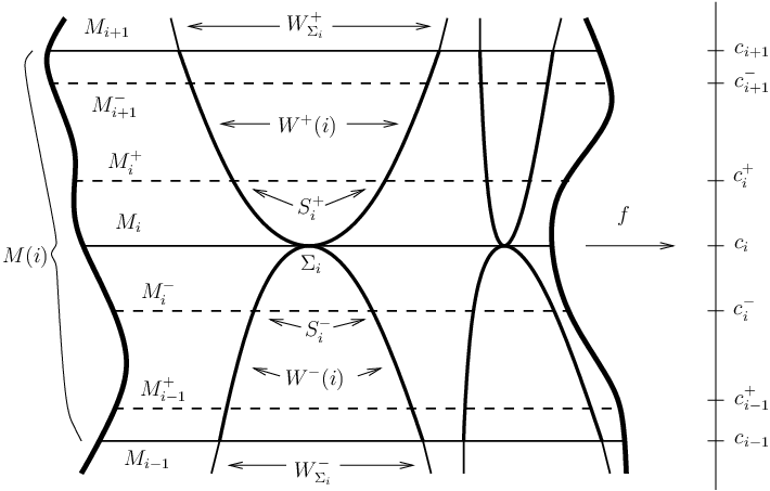

Let be the flow associated to the vector field on and consider the diffeomorphisms, see Figure 3,
and
as well as the submersion
The maps and extend to continuous maps
This can be seen from explicit formulae for and in the neighborhood of resp. , cf. [BFK]. Define
and denote by the canonical projections. One can verify the following
Lemma 4.
is a smooth submanifold with boundary diffeomorphic to . Precisely we have:
- (P1)
are diffeomorphisms.
- (P2)
The restriction of to is a diffeomorphism onto , each restricted to identifies with the projection onto .
Geometrically represents the space of all trajectories, possibly broken, from to .
Next we define
Equivalently, consists of pairs of points , , , which lie on the same possibly broken trajectory. Moreover let and denote the canonical projections. One can verify the following
Lemma 5.
is a smooth submanifold with boundary diffeomorphic to . Precisely we have:
- (Q1)
is a smooth bundle with fiber an open segment. is a diffeomorphism.
- (Q2)
The restriction of to is a diffeomorphism onto , i.e. resp. restricted to identifies with the projection onto resp. .
Since and are smooth manifolds with boundaries
| (34) |
and
| (35) |
are smooth manifolds with corners.
A.2. Proof of Theorem 3
We will equip
with the structure of a smooth manifold with corners. If the statement is empty. If there is nothing to check. So we suppose . We are going to apply Lemma 3.
Consider the smooth manifold with corners from (34) above, the smooth manifold and the smooth manifold . In order to define the maps and we consider
and
We also denote by resp. the restriction of resp. to resp. . Finally we set,
and
The verification of the transversally of and follows easily from (P1), (P2) and the Morse–Smale condition and is done exactly as in [BH01]. It is easy to see that identifies to as topological spaces and we leave this verification to the reader. The rest is straight forward.
A.3. Proof of Theorem 4
We are going equip the compact topological space with the structure of a smooth manifold with corners. Let us write . For any integer denote by . First we will put the structure of smooth manifold with corners on so that the restriction of is smooth. Second we check that and induce on the intersection the same smooth structure. These facts imply that has a canonical structure of smooth manifold with corners and that is a smooth map.
To accomplish first step we proceed in exactly the same way as in the proof of Theorem 3. Consider the smooth manifold with corners from (35), the smooth manifold and the smooth manifold . Define
and
Again we will apply Lemma 3. The verification of the transversality follows from (P1), (P2), (Q1), (Q2) and the Morse–Smale condition, exactly as explained in [BH01]. It is easy to see that identifies to . The rest is straight forward.
Appendix B Some homological algebra
B.1. Finite dimensional complexes
All vector spaces in this section are supposed to be finite dimensional and over a field of characteristics zero. For such a vector space we define its determinant by . If we have a short exact sequence of vector spaces we obtain a canonic isomorphism . This is constructed using a section to get an isomorphism . This induces an isomorphism which does not depend on the section.
If is a –graded vector space we define its determinant by . Here denotes the dual of . Note that we have a natural identification . Again, a short exact sequence of –graded vector spaces gives rise to a natural isomorphism by combining the isomorphisms for the even and the odd part.
Suppose is a –graded complex with a degree differential of odd degree and . Then we get three –graded vector spaces; , and . Moreover we get two short exact sequences of –graded vector spaces and . Here denotes the –graded vector space equipped with the opposite grading, and . Note that we have a natural isomorphism . The two short exact sequences provide natural isomorphisms
Together with they give rise to a natural isomorphism
| (36) |
Suppose we have a short exact sequence of –graded complexes . Its long exact sequence in cohomology
can be used to make the –graded vector space a –graded complex with vanishing cohomology. From (36) we thus obtain a natural isomorphism:
| (37) |
The following is a reformulation of a well known fact, which for instance can be found in [M66, Theorem 3.2].
Proposition 19.
Suppose is a short exact sequence of –graded complexes. Then the following diagram of canonic isomorphisms commutes up to sign:
Suppose is a –graded complex equipped with a filtration
which is preserved by the differential. We assume for sufficiently large and for sufficiently small. Moreover we assume that the filtration is compatible with the grading, that is where and . In this situation we have a spectral sequence converging to . Every is a –graded complex with differential . For the –term we have as –graded vector spaces. Here denotes the associated graded of considered as –graded complex, and its cohomology, a –graded vector space. We will not consider the –grading and inherit from the filtration. Applying (36) we obtain a canonic isomorphism . The cohomology inherits the structure of a –graded vector space with filtration from . Let denote the associated graded considered as –graded vector space. Again, we will not consider the –grading inherits. Since the spectral sequence converges we have a canonic isomorphism which provides us with a canonic isomorphism . Since we also have a canonic isomorphism for every . Also note that for sufficiently large.
The following can be found in [F92, Theorem 1.3], but see also [M69, Théorèm 4.4] for a more general result.
Proposition 20.
Let be a filtered –graded complex. Then the following diagram of canonic isomorphism commutes up to sign:
B.2. Finite dimensional complexes with scalar product
All vector spaces (complexes) in this section are suppose to be finite dimensional and over . We will work with –graded complexes and all determinant lines are understood in the graded sense. If a –graded complex comes with a scalar product we will assume , i.e. the even and the odd part are orthogonal. In such a situation , and are –graded vector spaces with scalar products. We let , , and denote the induced norms on , , and , respectively. Moreover let denote the adjoint of the differential and the Laplacian.
For a linear isomorphism between finite dimensional Euclidean spaces we set . For an arbitrary linear mapping between Euclidean spaces we let denote its restriction and thus have a volume . Moreover, if is a linear mapping between finite dimensional vector spaces we write for the product of non-zero eigen values. Clearly . For a –graded complex with scalar product define:
Remark 10.
Suppose we have a –graded complex with scalar product. It gives rise to a –graded complex with scalar product in the usual way. Let denote the Laplacian acting on . A two line computation using
and
shows
However, for this to make sense it is essential to have a –grading at hand.
Proposition 21.
Let be a –graded complex with scalar product. Then the canonic isomorphism maps to .
Proof.
The short exact sequence of –graded vector spaces induces an isomorphism which clearly maps to . The short exact sequence of –graded vector spaces induces an isomorphism which maps to . Putting this together we find via . ∎
Proposition 22.
Suppose is a short exact sequence of –graded complexes with compatible scalar products, i.e. is an isometry onto its image and carries the quotient scalar product. Then the canonic isomorphism
maps to .
Proof.
Let be a filtered –graded complex as considered in section B.1 and suppose is equipped with a scalar product. Then , and inherit scalar products in an obvious way.
Proposition 23.
Suppose is a filtered –graded complex with scalar product. Then the canonic isomorphism
maps to .
References
- [AB95] D.M. Austin and P.J. Braam, Morse–Bott theory and equivariant cohomology. The Floer memorial volume, 123–183. Progr. Math. 133, Birkhäuser, Basel, 1995.
- [BZ92] J.M. Bismut and W. Zhang, An extension of a theorem by Cheeger and Müller. With an appendix by F. Laudenbach. Astérisque 205(1992).
- [BZ94] J.M. Bismut and W. Zhang, Milnor and Ray–Singer metrics on the equivariant determinant of a flat vector bundle. Geom. Funct. Anal. 4(1994), 136–212.
- [BT82] R. Bott and L.W. Tu, Differential forms in algebraic topology. Graduate Texts in Mathematics 82. Springer–Verlag, New York–Berlin, 1982.
- [B99] D. Burghelea, Removing metric anomalies from Ray–Singer torsion, Lett. Math. Phys. 47(1999), 149–158.
- [BFK99] D. Burghelea, L. Friedlander and T. Kappeler, Torsions for manifolds with boundary and glueing formulas. Math. Nachr. 208(1999), 31–91.
- [BFK01] D. Burghelea, L. Friedlander and T. Kappeler, Relative torsion. Commun. Contemp. Math. 3(2001), 15–85.
- [BFK] D. Burghelea, L. Friedlander and T. Kappeler, Elementary Morse Theory, Lectures Notes in preparation.
- [BH01] D. Burghelea and S. Haller, On the topology and analysis of a closed one form. I (Novikov’s theory revisited). Essays on geometry and related topics, 133–175. Monogr. Enseign. Math. 38, Enseignement Math., Geneva, 2001.
- [BH] D. Burghelea and S. Haller, A Riemannian invariant, Euler structures and some topological applications, preprint math.DG/0310154.
- [BH04] …
- [C77] J. Cheeger, Analytic torsion and Reidemeister torsion, Proc. Nat. Acad. Sci. U.S.A. 74(1977), 2651–2654.
- [C79] J. Cheeger, Analytic torsion and the heat equation, Ann. of Math. 109(1979), 259–322.
- [D95] A. Dold, Lectures on algebraic topology. Reprint of the 1972 edition. Classics in Mathematics. Springer–Verlag, Berlin, 1995.
- [F92] D.S. Freed, Reidemeister torsion, spectral sequences, and Brieskorn spheres, J. Reine Angew. Math. 429(1992), 75–89.
- [LST98] W. Lück, T. Schick and T. Thielmann, Torsion and fibrations, J. Reine Angew. Math. 498(1998), 1–33.
- [M69] S. Maumary, Contributions à la théorie du type simple d’homotopie, Comment. Math. Helv. 44(1969), 410–437.
- [M66] J. Milnor, Whitehead torsion, Bull. Amer. Math. Soc. 72(1966), 358–426.
- [M78] W. Müller, Analytic torsion and -torsion of Riemannian manifolds, Adv. in Math. 28(1978), 233–305.
- [RS71] D.B. Ray and I.M. Singer, –torsion and the Laplacian on Riemannian manifolds, Adv. in Math. 7(1971), 145–210.
- [T90] V. Turaev, Euler structures, non-singular vector fields and Reidemeister-type torsions, Math. USSR–Izv. 34(1990), 627–662.
- [T02] V. Turaev, Torsions of –dimensional manifolds. Progress in Mathematics 208. Birkhäuser Verlag, Basel, 2002.