跳到论文正文
W Papers独立论文阅读器 arXiv:math/0408426 论文正文 计算阅读时间 · 0%
引用这篇论文根据当前论文元数据生成,正式投稿前建议核对。


License: Assumed arXiv.org perpetual non-exclusive license
arXiv:math/0408426v3 [math.AG] 09 Oct 2007

A mathematical theory of the topological vertex

Jun Li Address: Department of Mathematics, Stanford University, Stanford, CA 94305, USA Email address: jli@math.stanford.edu , Chiu-Chu Melissa Liu Address: Department of Mathematics, Northwestern University, Evanston, IL 60208, USA Email address: ccliu@math.northwestern.edu , Kefeng Liu Address: Center of Mathematical Sciences, Zhejiang University, Hangzhou, China; Department of Mathematics, University of California at Los Angeles, Los Angeles, CA 90095-1555, USA Email address: liu@cms.zju.edu.cn, liu@math.ucla.edu and Jian Zhou Address: Department of Mathematical Sciences, Tsinghua University, Beijing, 100084, China Email address: jzhou@math.tsinghua.edu.cn
Abstract.

We have developed a mathematical theory of the topological vertex—a theory that was originally proposed by M. Aganagic, A. Klemm, M. Mariño, and C. Vafa on effectively computing Gromov-Witten invariants of smooth toric Calabi-Yau threefolds derived from duality between open string theory of smooth Calabi-Yau threefolds and Chern-Simons theory on three manifolds.

1. Introduction

In [1], M. Aganagic, A. Klemm, M. Mariño and C. Vafa proposed a theory on computing Gromov-Witten invariants in all genera of any smooth toric Calabi-Yau threefold derived from duality between open string theory of smooth Calabi-Yau threefolds and Chern-Simons theory on 3-manifolds. In summary their theory says that

  1. O1.

    There exist certain open Gromov-Witten invariants counting holomorphic maps from bordered Riemann surfaces to ℂ3\mathbb{C}^{3} with boundary mapped to three specific Lagrangian submanifolds. The topological vertex

    Cμ→​(λ,𝐧)C_{{\vec{\mu}}}(\lambda;\mathbf{n})

    is a generating function of such invariants; it depends on a triple of partitions μ→=(μ1,μ2,μ3){\vec{\mu}}=({{\mu}^{1},{\mu}^{2},{\mu}^{3}}) and a triple of integers 𝐧=(n1,n2,n3)\mathbf{n}=({n}_{1},{n}_{2},{n}_{3}).

  2. O2.

    The Gromov-Witten invariants of any smooth toric Calabi-Yau threefold can be expressed in terms of Cμ→​(λ,𝐧)C_{{\vec{\mu}}}(\lambda;\mathbf{n}) by explicit gluing algorithms.

  3. O3.

    By the duality between Chern-Simons theory and Gromov-Witten theory, the topological vertex is given by

    (1.1) Cμ→​(λ,𝐧)=q12​(∑i=13κνi​ni)​𝒲μ→​(q),C_{{\vec{\mu}}}(\lambda;\mathbf{n})=q^{\frac{1}{2}(\sum_{i=1}^{3}\kappa_{\nu^{i}}n_{i})}{\cal W}_{\vec{\mu}}(q),

    where q=e−1​λq=e^{\sqrt{-1}\lambda} and 𝒲μ→​(q){\cal W}_{\vec{\mu}}(q) is a combinatorial expression related to the Chern-Simons link invariants of a particular link. (cf. Section 2.1.)

As was demonstrated in the work of many, for instance [45, 21, 22], this algorithm is extremely efficient in deriving the structure result of the Gromov-Witten invariants of toric Calabi-Yau threefolds.

The purpose of this paper is to provide a mathematical theory for this algorithm. To achieve this, we need to provide a mathematical definition of the open Gromov-Witten invariants referred to in O1; secondly, we need to establish the gluing algorithms O2; finally, the duality O3 must be established mathematically.

In this paper, we shall complete the first two steps as outlined. Our theory is based on relative Gromov-Witten theory [26, 18, 19, 24, 25]. Our results can be summarized as follows.

  1. R1.

    We introduce the notion of formal toric Calabi-Yau (FTCY) graphs, which is a refinement and generalization of the graph associated to a toric Calabi-Yau threefold. An FTCY graph Γ\Gamma determines a relative FTCY threefold Yrel=(Y^,D^)Y^{\mathrm{rel}}=(\hat{Y},\hat{D}); it can be degenerated to indecomposable ones.

  2. R2.

    We define formal relative Gromov-Witten invariants for relative FTCY threefolds (Theorem 4.8). These invariants include as special cases Gromov-Witten invariants of smooth toric Calabi-Yau threefolds.

  3. R3.

    We show that the formal relative Gromov-Witten invariants in R2 satisfy the degeneration formula of relative Gromov-Witten invariants of projective varieties (Theorem 7.5).

  4. R4.

    Any smooth relative FTCY threefold can be degenerated to indecomposable ones, whose isomorphism classes are determined by a triple of integers 𝐧=(n1,n2,n3)\mathbf{n}=({n}_{1},{n}_{2},{n}_{3}). By degeneration formula, the formal relative Gromov-Witten invariants in R2 can be expressed in terms of the generating function C~μ→​(λ,𝐧)\tilde{C}_{{\vec{\mu}}}(\lambda;\mathbf{n}) of that of an indecomposable FTCY threefold (Proposition 7.4). This degeneration formula coincides with the gluing algorithms described in O2.

  5. R5.

    We evaluate C~μ→​(λ,𝐧)\tilde{C}_{{\vec{\mu}}}(\lambda;\mathbf{n}) (Proposition 6.5, Theorem 8.1):

    (1.2) C~μ→​(λ,𝐧)=q12​(∑i=13κνi​ni)​𝒲~μ→​(q),\tilde{C}_{{\vec{\mu}}}(\lambda;\mathbf{n})=q^{\frac{1}{2}(\sum_{i=1}^{3}\kappa_{\nu^{i}}n_{i})}{\tilde{\cal W}}_{\vec{\mu}}(q),

    where 𝒲~μ→​(q){\tilde{\cal W}}_{\vec{\mu}}(q) is a combinatorial expression defined by (2.5) in Section 2.1.

In R4, we shall define C~μ→​(λ,𝐧)\tilde{C}_{\vec{\mu}}(\lambda;\mathbf{n}) as local relative Gromov-Witten invariants of a formal Calabi-Yau (Z^,D^)(\hat{Z},\hat{D}) that is the infinitesimal neighborhood of a configuration C1∪C2∪C3C_{1}\cup C_{2}\cup C_{3} of three ℙ1\mathbb{P}^{1}’s meeting at a point p0p_{0} in a relative Calabi-Yau threefold (Z,D)(Z,D); the stable maps have ramification partition μi\mu^{i} around the relative divisor DD. Since Z^\hat{Z} is formal, we shall define the local invariants C~μ→​(λ,𝐧)\tilde{C}_{{\vec{\mu}}}(\lambda;\mathbf{n}) via localization formula. The most technical part of the paper is to show that such local invariants exist as topological invariants; namely they are rational numbers independent of equivariant parameters (Theorem 5.2, invariance of the topological vertex).

Our results R1-R5, together with a conjectural identity 𝒲~μ→​(q)=𝒲μ→​(q){\tilde{\cal W}}_{\vec{\mu}}(q)={\cal W}_{\vec{\mu}}(q) (Conjecture 8.3), will provide a complete mathematical theory of the topological vertex theory. The conjecture holds when one of the partitions, say μ3\mu^{3}, is empty (Corollary 8.8); it also holds for all low degree cases we have checked.

By virtual localization, C~μ→​(λ,𝐧)\tilde{C}_{{\vec{\mu}}}(\lambda;\mathbf{n}) can be expressed in terms of Hodge integrals (Proposition 6.6), which combined with (1.2) provides us a formula of a generating function Gμ→∙​(λ,𝐰)G^{\bullet}_{\vec{\mu}}(\lambda;\mathbf{w}) of the three-partition Hodge integrals (Theorem 8.2):

(1.3) Gμ→∙​(λ,𝐰)=∑|νi|=|μi|∏i=13χνi​(μi)zμi​q12​(∑i=13κνi​wi+1wi)​𝒲~ν→​(q).G^{\bullet}_{\vec{\mu}}(\lambda;\mathbf{w})=\sum_{|\nu^{i}|=|\mu^{i}|}\prod_{i=1}^{3}\frac{\chi_{\nu^{i}}(\mu^{i})}{z_{\mu^{i}}}q^{\frac{1}{2}(\sum_{i=1}^{3}\kappa_{\nu^{i}}\frac{w_{i+1}}{w_{i}})}\tilde{{\cal W}}_{\vec{\nu}}(q).

(See Section 2 for precise definitions involved in (1.3)). This generalizes a formula of two-partition Hodge integrals (Theorem 8.7) proved in [31]. Our evaluation of three-partition Hodge integrals, thus C~μ→​(λ,𝐧)\tilde{C}_{{\vec{\mu}}}(\lambda;\mathbf{n}), relies on the cut-and-join equations of three partition Hodge integrals, which turn out to be equivalent to the invariance of the topological vertex mentioned above. Indeed, the cut-and-join equations are so strong that they reduce the evaluation of general three-partition Hodge integrals first to the case where μ3=∅\mu^{3}=\emptyset, and eventually to the case where μ1=(d)\mu^{1}=(d) and μ2=μ3=∅\mu^{2}=\mu^{3}=\emptyset.

An important class of toric Calabi-Yau threefolds consists of local toric surfaces in a Calabi-Yau threefold; they are the total space of the canonical line bundle of a projective toric surface (e.g. 𝒪ℙ2​(−3){\cal O}_{\mathbb{P}^{2}}(-3)). In this case, only C~μ1,μ2,∅​(λ,𝐧)\tilde{C}_{\mu^{1},\mu^{2},\emptyset}(\lambda;\mathbf{n}) (or two-partition Hodge integrals) are involved. The algorithm in this case was described in [2]; explicit formula was given in [17] and derived in [50] by localization, using the formula of two-partition Hodge integrals.

It is worth mentioning that, assuming the existence of Cμ→​(λ,𝐧)C_{\vec{\mu}}(\lambda;\mathbf{n}) and the validity of open string virtual localization, Diaconescu and Florea related Cμ→​(λ,n1,n2,n3)C_{\vec{\mu}}(\lambda;{{n}_{1},{n}_{2},{n}_{3}}) (at certain fractional nin_{i}) to three-partition Hodge integrals, and derived the gluing algorithms in O2 by localization [6].

Maulik, Nekrasov, Okounkov, and Pandharipande conjectured a correspondence between the Gromov-Witten and Donaldson-Thomas theories for any non-singular projective threefold [36, 37]. This correspondence can also be formulated for certain non-compact threefolds in the presence of a torus action; the correspondence for toric Calabi-Yau threefolds is equivalent to the validity of the topological vertex [36, 42]. For non-Calabi-Yau toric threefolds the building block is the equivariant vertex (see [36, 37, 43, 44]) which depends on equivariant parameters11 1 During the revision of this paper, Maulik, Oblomkov, Okounkov, and Pandharipande announced a proof of GW/DT correspondence for all toric threefolds [38]..

The rest of this paper is organized as follows. In Section 2, we recall some definitions and previous results, and introduce some generating functions. R1 is carried out in Section 3. R2 is carried out in Section 4; the case when the relative FTCY threefold is indecomposable gives the mathematical definition of topological vertex, and the proof of its invariance (Theorem 5.2) is given in Section 5. In Section 6, we express the topological vertex in terms of three-partition Hodge integrals and double Hurwitz numbers. In Section 7, we establish R3 and R4. In Section 8, we derive the combinatorial expression in R5. Some examples of the identity 𝒲μ→​(q)=𝒲~μ→​(q){\cal W}_{\vec{\mu}}(q)={\tilde{\cal W}}_{\vec{\mu}}(q) are listed in Section 8.4.

Acknowledgments.

We wish to thank A. Aganagic, A. Klemm, M. Mariño, and C. Vafa for their explanation of [1] in public lectures and private conversations. We also wish to thank S. Katz and E. Diaconescu for helpful conversations. We thank A. Klemm for writing a maple program which computes both 𝒲μ→​(q){\cal W}_{\vec{\mu}}(q) and 𝒲~μ→​(q){\tilde{\cal W}}_{\vec{\mu}}(q). The first author is supported by NSF grant DMS-0200477 and DMS-0244550. The third author is supported by the NSF and the Guggenheim foundation.

2. Definitions and Previous Results

In this section, we recall some definitions and previous results, and introduce some generating functions. We begin with the partitions and representations of symmetric groups.

2.1. Partitions and Representations of Symmetric Groups

Recall that a partition μ\mu of a nonnegative integer dd is a sequence of positive integers

μ=(μ1≥μ2≥⋯≥μh>0)such thatd=μ1+…+μh.\mu=(\mu_{1}\geq\mu_{2}\geq\cdots\geq\mu_{h}>0)\quad\text{such that}\ \ d=\mu_{1}+\ldots+\mu_{h}.

We write μ⊢d\mu\vdash d or |μ|=d|\mu|=d, and call ℓ⁡(μ)=h\ell(\mu)=h the length of the partition. For convenience, we denote by ∅\emptyset the empty partition; thus |∅|=ℓ⁡(∅)=0|\emptyset|=\ell(\emptyset)=0. The order of Aut⁡(μ)\Aut(\mu), the group of permutations of μ1,μ2,⋯\mu_{1},\mu_{2},\cdots that leave μ\mu fixed, is

|Aut⁡(μ)|=∏jmj​(μ)!,wheremj​(μ)=#⁡{i:μi=j}.|\Aut(\mu)|=\prod_{j}m_{j}(\mu)!,\quad\text{where}\quad m_{j}(\mu)=\#\{i:\mu_{i}=j\}.

The transpose of μ\mu is a partition μt\mu^{t} defined by mi​(μt)=μi−μi+1m_{i}(\mu^{t})=\mu_{i}-\mu_{i+1}. Note that

|μt|=|μ|,(μt)t=μ,ℓ⁡(μt)=μ1.|\mu^{t}|=|\mu|,\ \,(\mu^{t})^{t}=\mu,\ \ \ell(\mu^{t})=\mu_{1}.

A partition μ\mu also corresponds to a conjugacy class in SdS_{d}, where SdS_{d} is the permutation group of d=|μ|d=|\mu| elements in the obvious way. With this understanding, the cardinality zμz_{\mu} of the centralizer of any element in this conjugacy class is of the form,

zμ=aμ|Aut(μ)|,whereaμ=μ1⋯μℓ⁡(μ).z_{\mu}=a_{\mu}|\Aut(\mu)|,\quad\text{where}\ a_{\mu}=\mu_{1}\cdots\mu_{\ell(\mu)}.

We let 𝒫{\cal P} denote the set of partitions; we let

𝒫+=𝒫−{∅},𝒫+2=𝒫2−{(∅,∅)},𝒫+3=𝒫3−{(∅,∅,∅)}.{\cal P}_{+}={\cal P}-\{\emptyset\},\ \ {\cal P}^{2}_{+}={\cal P}^{2}-\{(\emptyset,\emptyset)\},\ \ {\cal P}^{3}_{+}={\cal P}^{3}-\{(\emptyset,\emptyset,\emptyset)\}.

Given a triple of partitions μ→=(μ1,μ2,μ3)∈𝒫3{\vec{\mu}}=({{\mu}^{1},{\mu}^{2},{\mu}^{3}})\in{\cal P}^{3}, we define

ℓ⁡(μ→)=∑i=13ℓ⁡(μi),Aut⁡(μ→)=∏i=13Aut⁡(μi).\ell({\vec{\mu}})=\sum_{i=1}^{3}\ell(\mu^{i}),\ \ \Aut({\vec{\mu}})=\prod_{i=1}^{3}\Aut(\mu^{i}).

For any partition ν\nu, we let χν\chi_{\nu} denote the irreducible character of S|ν|S_{|\nu|} indexed by ν\nu, and let χν​(μ)\chi_{\nu}(\mu) be the value of χν\chi_{\nu} on the conjugacy class determined by the partition μ\mu. Recall that the Schur functions sμs_{\mu} are related to the Newton functions pi​(x)=x1i+x2i+⋯p_{i}(x)=x_{1}^{i}+x_{2}^{i}+\cdots by

sμ​(x)=∑|ν|=|μ|χμ​(ν)zν​pν​(x),x=(x1,x2,…).s_{\mu}(x)=\sum_{|\nu|=|\mu|}\frac{\chi_{\mu}(\nu)}{z_{\nu}}p_{\nu}(x),\quad x=(x_{1},x_{2},\ldots).

The Littlewood-Richardson coefficients cμ​νηc_{\mu\nu}^{\eta}, which are nonnegative integers, and skew Schur functions are determined according to the rules

sμ​sν=∑ηcμ​νη​sη​sη/μ=∑νcμ​νη​sν.s_{\mu}s_{\nu}=\sum_{\eta}c^{\eta}_{\mu\nu}s_{\eta}s_{\eta/\mu}=\sum_{\nu}c^{\eta}_{\mu\nu}s_{\nu}.

In order to define the combinatorial expressions 𝒲μ→​(q){\cal W}_{\vec{\mu}}(q) and 𝒲~μ→​(q)\tilde{{\cal W}}_{\vec{\mu}}(q) in O3 and R5 in the introduction (Section 1), we need to introduce more notation. We define [m]=qm/2−q−m/2[m]=q^{m/2}-q^{-m/2}, and define

(2.1) κμ=∑i=1ℓ⁡(μ)μi​(μi−2​i+1),\kappa_{\mu}=\sum_{i=1}^{\ell(\mu)}\mu_{i}(\mu_{i}-2i+1),

which for transpose partitions satisfies κμt=−κμ\kappa_{\mu^{t}}=-\kappa_{\mu}.

We define

(2.2) 𝒲μ​(q)=qκμ/4​∏1≤i<j≤ℓ⁡(μ)[μi−μj+j−i][j−i]​∏i=1ℓ⁡(μ)∏v=1μi1[v−i+ℓ⁡(μ)]{\cal W}_{\mu}(q)=q^{\kappa_{\mu}/4}\prod_{1\leq i<j\leq\ell(\mu)}\frac{[\mu_{i}-\mu_{j}+j-i]}{[j-i]}\prod_{i=1}^{\ell(\mu)}\prod_{v=1}^{\mu_{i}}\frac{1}{[v-i+\ell(\mu)]}

and define

(2.3) 𝒲μ,ν​(q)=q|ν|/2​𝒲μ​(q)⋅sν​(ℰμ​(q,t)),{\cal W}_{\mu,\nu}(q)=q^{|\nu|/2}{\cal W}_{\mu}(q)\cdot s_{\nu}({\cal E}_{\mu}(q,t)),

where

ℰμ​(q,t)=∏j=1l⁡(μ)1+qμj−j​t1+q−j​t⋅(1+∑n=1∞tn∏i=1n(qi−1)).{\cal E}_{\mu}(q,t)=\prod_{j=1}^{l(\mu)}\frac{1+q^{\mu_{j}-j}t}{1+q^{-j}t}\cdot\biggl(1+\sum_{n=1}^{\infty}\frac{t^{n}}{\prod_{i=1}^{n}(q^{i}-1)}\biggr).

We also denote

cρ1​(ρ3)tμ1​(μ3)t=∑ηcη​ρ1μ1​cη​(ρ3)t(μ3)t.c_{\rho^{1}(\rho^{3})^{t}}^{\mu^{1}(\mu^{3})^{t}}=\sum_{\eta}c_{\eta\rho^{1}}^{\mu^{1}}c_{\eta(\rho^{3})^{t}}^{(\mu^{3})^{t}}.
Definition 2.1.

For μ→=(μ1,μ2,μ3){\vec{\mu}}=({{\mu}^{1},{\mu}^{2},{\mu}^{3}}), we define

(2.4) 𝒲μ→​(q)=qκμ2/2+κμ3/2​∑ρ1,ρ3cρ1​(ρ3)tμ1​(μ3)t​𝒲(μ2)t​ρ1​(q)​𝒲μ2​(ρ3)t​(q)𝒲μ2​(q).{\cal W}_{{\vec{\mu}}}(q)=q^{\kappa_{\mu^{2}}/2+\kappa_{\mu^{3}}/2}\sum_{\rho^{1},\rho^{3}}c_{\rho^{1}(\rho^{3})^{t}}^{\mu^{1}(\mu^{3})^{t}}\frac{{\cal W}_{(\mu^{2})^{t}\rho^{1}}(q){\cal W}_{\mu^{2}(\rho^{3})^{t}}(q)}{{\cal W}_{\mu^{2}}(q)}\,.
Definition 2.2.

For a partition μ=(μ1≥μ2≥⋯)\mu=(\mu_{1}\geq\mu_{2}\geq\cdots) we let 2​μ2\mu be the partition (2​μ1≥2​μ2≥⋯)(2\mu_{1}\geq 2\mu_{2}\geq\cdots). For ρ→=(ρ1,ρ2,ρ3)\vec{\rho}=({{\rho}^{1},{\rho}^{2},{\rho}^{3}}), we define

(2.5) 𝒲~ρ→​(q)=\displaystyle\tilde{{\cal W}}_{\vec{\rho}}(q)= q−(κρ1−2κρ2−12κρ3)/2∑ν+,η1,ν1,η3,ν3cν+(ν1)t​ρ2c(η1)t​ν1ρ1cη3​(ν3)tρ3\displaystyle q^{-(\kappa_{\rho^{1}}-2\kappa_{\rho^{2}}-\frac{1}{2}\kappa_{\rho^{3}})/2}\sum_{\nu^{+},\eta^{1},\nu^{1},\eta^{3},\nu^{3}}c^{\nu^{+}}_{(\nu^{1})^{t}\rho^{2}}c_{(\eta^{1})^{t}\nu^{1}}^{\rho^{1}}c_{\eta^{3}(\nu^{3})^{t}}^{\rho^{3}}
⋅q(−2​κν+−κν32)/2​𝒲ν+,ν3​(q)​∑μ1zμ​χη1​(μ)​χη3​(2​μ).\displaystyle\cdot q^{(-2\kappa_{\nu^{+}}-\frac{\kappa_{\nu^{3}}}{2})/2}{\cal W}_{\nu^{+},\nu^{3}}(q)\sum_{\mu}\frac{1}{z_{\mu}}\chi_{\eta^{1}}(\mu)\chi_{\eta^{3}}(2\mu)\,.

We have the following identities (see [51]):

(2.6) 𝒲μ,ν,∅​(q)=𝒲∅,μ,ν​(q)=𝒲ν,∅,μ​(q)=qκν/2​𝒲μ,(ν)t​(q).{\cal W}_{\mu,\nu,\emptyset}(q)={\cal W}_{\emptyset,\mu,\nu}(q)={\cal W}_{\nu,\emptyset,\mu}(q)=q^{\kappa_{\nu}/2}{\cal W}_{\mu,(\nu)^{t}}(q).
(2.7) 𝒲μ,ν​(q)=𝒲ν,μ​(q),𝒲μ,∅​(q)=𝒲μ​(q).{\cal W}_{\mu,\nu}(q)={\cal W}_{\nu,\mu}(q),\quad{\cal W}_{\mu,\emptyset}(q)={\cal W}_{\mu}(q).

2.2. Double Hurwitz Numbers

We now come to the generating function of the double Hurwitz numbers. Let μ+,μ−\mu^{+},\mu^{-} be partitions of dd; let Hχ,μ+,μ−∙H^{\bullet}_{\chi,\mu^{+},\mu^{-}} be the weighted counts of Hurwitz covers of the sphere of the type (μ+,μ−)(\mu^{+},\mu^{-}) by possibly disconnected Riemann surfaces of Euler characteristic χ\chi. We form the generating function

Φμ+,μ−∙​(λ)=∑χλ−χ+ℓ⁡(μ+)+ℓ⁡(μ−)​Hχ,μ+,μ−∙(−χ+ℓ⁡(μ+)+ℓ⁡(μ−))!.\Phi^{\bullet}_{\mu^{+},\mu^{-}}(\lambda)=\sum_{\chi}\lambda^{-\chi+\ell(\mu^{+})+\ell(\mu^{-})}\frac{H^{\bullet}_{\chi,\mu^{+},\mu^{-}}}{(-\chi+\ell(\mu^{+})+\ell(\mu^{-}))!}.

By Burnside formula,

(2.8) Φμ+,μ−∙​(λ)=∑|ν|=deκν​λ/2​χν​(μ+)zμ+​χν​(μ−)zμ−.\Phi^{\bullet}_{\mu^{+},\mu^{-}}(\lambda)=\sum_{|\nu|=d}e^{\kappa_{\nu}\lambda/2}\frac{\chi_{\nu}(\mu^{+})}{z_{\mu^{+}}}\frac{\chi_{\nu}(\mu^{-})}{z_{\mu^{-}}}.

Using the orthogonality of characters

(2.9) ∑ρχμ​(ρ)​χν​(ρ)zρ=δμ​ν,\sum_{\rho}\frac{\chi_{\mu}(\rho)\chi_{\nu}(\rho)}{z_{\rho}}=\delta_{\mu\nu},

it is straightforward to check that (2.8) implies the following two identities:

(2.10) Φμ+,μ−∙​(λ1+λ2)=∑|ν|=dΦμ+,ν∙​(λ1)​zν​Φν,μ−∙​(λ2)\Phi^{\bullet}_{\mu^{+},\mu^{-}}(\lambda_{1}+\lambda_{2})=\sum_{|\nu|=d}\Phi^{\bullet}_{\mu^{+},\nu}(\lambda_{1})z_{\nu}\Phi^{\bullet}_{\nu,\mu^{-}}(\lambda_{2})

and

(2.11) Φμ+,μ−∙​(0)=δμ+​μ−zμ+.\Phi^{\bullet}_{\mu^{+},\mu^{-}}(0)=\frac{\delta_{\mu^{+}\mu^{-}}}{z_{\mu^{+}}}.

Equation (2.10) is a sum formula for double Hurwitz numbers; Equation (2.11) gives the initial values for the double Hurwitz numbers.

Following [12, 13, 14], we introduce a differential equation that has a generating function of Φμ+,μ−∙\Phi^{\bullet}_{\mu^{+},\mu^{-}} as its unique solution which satisfies the initial condition (2.11). This equation is similar to [13, Lemma 2.2] and [14, Lemma 3.1].

We let p±=(p1±,p2±,…)p^{\pm}=(p^{\pm}_{1},p^{\pm}_{2},\ldots) be formal variables, and for a partition μ\mu we let p±μ=p±μ1⋯p±μℓ⁡(μ)p^{\pm}_{\mu}=p^{\pm}_{\mu_{1}}\cdots p^{\pm}_{\mu_{\ell(\mu)}}. We then define a generating function

Φ∙​(λ,p+,p−)=1+∑d=1∞∑|μ±|=dΦμ+,μ−∙​(λ)​pμ++​pμ−−,\Phi^{\bullet}(\lambda;p^{+},p^{-})=1+\sum_{d=1}^{\infty}\sum_{|\mu^{\pm}|=d}\Phi^{\bullet}_{\mu^{+},\mu^{-}}(\lambda)p^{+}_{\mu^{+}}p^{-}_{\mu^{-}},

and differential operators

C±=∑j,k(j+k)​pj±​pk±​∂∂pj+k±,J±=∑j,kj​k​pj+k±​∂2∂pj±​∂pk±.C^{\pm}=\sum_{j,k}(j+k)p^{\pm}_{j}p^{\pm}_{k}\frac{\partial}{\partial p^{\pm}_{j+k}},\quad J^{\pm}=\sum_{j,k}jkp^{\pm}_{j+k}\frac{\partial^{2}}{\partial p^{\pm}_{j}\partial p^{\pm}_{k}}.

They form a cut-and-join equation for double Hurwitz numbers:

(2.12) ∂Φ∙∂λ=12​(C++J+)​Φ∙=12​(C−+J−)​Φ∙.\frac{\partial\Phi^{\bullet}}{\partial\lambda}=\frac{1}{2}(C^{+}+J^{+})\Phi^{\bullet}=\frac{1}{2}(C^{-}+J^{-})\Phi^{\bullet}.

The generating function Φ∙​(λ,p+,p−)\Phi^{\bullet}(\lambda;p^{+},p^{-}) is the unique solution to this system satisfying the initial value

Φ∙​(0,p+,p−)=1+∑μ∈𝒫+pμ+​pμ−zμ.\Phi^{\bullet}(0;p^{+},p^{-})=1+\sum_{\mu\in{\cal P}^{+}}\frac{p^{+}_{\mu}p^{-}_{\mu}}{z_{\mu}}.

2.3. Three-Partition Hodge Integrals

We shall introduce three-partition Hodge integrals in this subsection.

For the three-partition Hodge integrals we need to work with Deligne-Mumford moduli stack ℳg,n{{\cal M}}_{g,n} of stable nn-pointed nodal curves of genus gg. Over this moduli stack, we let π:ℳg,n+1→ℳg,n\pi:{{\cal M}}_{g,n+1}\to{{\cal M}}_{g,n} be the universal curve, let si:ℳg,n→ℳg,n+1s_{i}:{{\cal M}}_{g,n}\to{{\cal M}}_{g,n+1} be its section that corresponds to the ii-th marked points of the family, and let ωπ\omega_{\pi} be the relative dualizing sheaf. The commonly known λ\lambda classes and the ψ\psi-class are defined using these morphisms. One forms the Hodge bundle 𝔼=π∗​ωπ\mathbb{E}=\pi_{*}\omega_{\pi}; its jj-th Chern class λj=cj​(𝔼)\lambda_{j}=c_{j}(\mathbb{E}) is the λ\lambda-class. One then form the pull back line bundle 𝕃i=si∗​ωπ\mathbb{L}_{i}=s_{i}^{*}\omega_{\pi}; its first Chern class ψi=c1​(𝕃i)\psi_{i}=c_{1}(\mathbb{L}_{i}) is the ψ\psi-class. A Hodge integral is then an integral of the form

∫ℳg,nψ1j1⋯ψnjnλ1k1⋯λgkg.\int_{{{\cal M}}_{g,n}}\psi_{1}^{j_{1}}\cdots\psi_{n}^{j_{n}}\lambda_{1}^{k_{1}}\cdots\lambda_{g}^{k_{g}}.

We now introduce three-partition Hodge integrals. Let w1,w2,w3{{w}_{1},{w}_{2},{w}_{3}} be formal variables. In this Subsection, and in Section 6, 7, 8, we use the following convention:

(2.13) 𝐰=(w1,w2,w3),w1+w2+w3=0,w4=w1.\mathbf{w}=({{w}_{1},{w}_{2},{w}_{3}}),\quad w_{1}+w_{2}+w_{3}=0,\quad w_{4}=w_{1}.

For μ→=(μ1,μ2,μ3)∈𝒫+3{\vec{\mu}}=({{\mu}^{1},{\mu}^{2},{\mu}^{3}})\in{\cal P}^{3}_{+}, we let

dμ→1=0,dμ→2=ℓ⁡(μ1),dμ→3=ℓ⁡(μ1)+ℓ⁡(μ2).d^{1}_{\vec{\mu}}=0,\quad d^{2}_{\vec{\mu}}=\ell(\mu^{1}),\quad d^{3}_{\vec{\mu}}=\ell(\mu^{1})+\ell(\mu^{2}).

We define the three-partition Hodge integral to be

(2.14) Gg,μ→​(𝐰)=(−−1)ℓ⁡(μ→)|Aut⁡(μ→)|​∏i=13∏j=1ℓ⁡(μi)∏a=1μji−1(μji​wi+1+a​wi)(μji−1)!​wiμji−1​∫ℳg,ℓ⁡(μ→)∏i=13Λg∨​(wi)​wiℓ⁡(μ→)−1∏j=1ℓ⁡(μi)(wi​(wi−μji​ψdμ→i+j))G_{g,{\vec{\mu}}}(\mathbf{w})=\frac{(-\sqrt{-1})^{\ell({\vec{\mu}})}}{|\Aut({\vec{\mu}})|}\prod_{i=1}^{3}\prod_{j=1}^{\ell(\mu^{i})}\frac{\prod_{a=1}^{\mu^{i}_{j}-1}(\mu^{i}_{j}w_{i+1}+aw_{i})}{(\mu^{i}_{j}-1)!w_{i}^{\mu^{i}_{j}-1}}\int_{{{\cal M}}_{g,\ell({\vec{\mu}})}}\prod_{i=1}^{3}\frac{\Lambda_{g}^{\vee}(w_{i})w_{i}^{\ell({\vec{\mu}})-1}}{\prod_{j=1}^{\ell(\mu^{i})}(w_{i}(w_{i}-\mu^{i}_{j}\psi_{d^{i}_{\vec{\mu}}+j}))}

where Λg∨​(u)=ug−λ1​ug−1+⋯+(−1)g​λg\Lambda_{g}^{\vee}(u)=u^{g}-\lambda_{1}u^{g-1}+\cdots+(-1)^{g}\lambda_{g}.

It is clear from the definition that Gg,μ→​(𝐰)G_{g,{\vec{\mu}}}(\mathbf{w}) obeys the cyclic symmetry:

(2.15) Gg,μ1,μ2,μ3​(w1,w2,w3)=Gg,μ2,μ3,μ1​(w2,w3,w1).G_{g,\mu^{1},\mu^{2},\mu^{3}}({{w}_{1},{w}_{2},{w}_{3}})=G_{g,\mu^{2},\mu^{3},\mu^{1}}(w_{2},w_{3},w_{1}).

Note −1ℓ⁡(μ→)​Gg,μ→​(𝐰)\sqrt{-1}^{\ell({\vec{\mu}})}G_{g,{\vec{\mu}}}(\mathbf{w}) is a rational function in w1,w2,w3w_{1},w_{2},w_{3} with ℚ\mathbb{Q}-coefficients, and is homogeneous of degree 00, so it suffices to work with 𝐰=(1,τ,−τ−1)\mathbf{w}=(1,\tau,-\tau-1). For such weights, we shall write

Gg,μ→​(τ)=Gg,μ→​(1,τ,−τ−1).G_{g,{\vec{\mu}}}(\tau)=G_{g,{\vec{\mu}}}(1,\tau,-\tau-1).

Then (2.15) becomes

Gg,μ1,μ2,μ3​(τ)=Gg,μ2,μ3,μ2​(−1−1τ)=Gg,μ3,μ1,μ2​(−1τ+1).G_{g,{{\mu}^{1},{\mu}^{2},{\mu}^{3}}}(\tau)=G_{g,\mu^{2},\mu^{3},\mu^{2}}(-1-\frac{1}{\tau})=G_{g,\mu^{3},\mu^{1},\mu^{2}}(\frac{-1}{\tau+1}).

We now form three-partition generating functions. We let λ\lambda and pi=(p1i,p2i,…)p^{i}=(p^{i}_{1},p^{i}_{2},\ldots) be formal variables; given a partition μ\mu we define piμ=pi1⋯piℓ⁡(μ)p^{i}_{\mu}=p^{i}_{1}\cdots p^{i}_{\ell(\mu)}; (note p∅i=1p^{i}_{\emptyset}=1); for p1p^{1}, p2p^{2} and p3p^{3}, we abbreviate

𝐩=(p1,p2,p3)​𝐩μ→=pμ11​pμ22​pμ33.\mathbf{p}=({{p}^{1},{p}^{2},{p}^{3}})\mathbf{p}_{\vec{\mu}}=p^{1}_{\mu^{1}}p^{2}_{\mu^{2}}p^{3}_{\mu^{3}}.

The generating functions are

Gμ→​(λ,𝐰)=∑g=0∞λ2​g−2+ℓ⁡(μ→)​Gg,μ→​(𝐰)andG⁡(λ,𝐩,𝐰)=∑μ→∈𝒫+3Gμ→​(λ,𝐰)​𝐩μ→.G_{\vec{\mu}}(\lambda;\mathbf{w})=\sum_{g=0}^{\infty}\lambda^{2g-2+\ell({\vec{\mu}})}G_{g,{\vec{\mu}}}(\mathbf{w})\quad\textup{and}\quad G(\lambda;\mathbf{p};\mathbf{w})=\sum_{{\vec{\mu}}\in{\cal P}^{3}_{+}}G_{\vec{\mu}}(\lambda;\mathbf{w})\mathbf{p}_{\vec{\mu}}.

The generating fucntions for not necessarily connected domain curves are

(2.16) G∙​(λ,𝐩,𝐰)=exp⁡(G⁡(λ,𝐩,𝐰))=1+∑μ→∈𝒫+3Gμ→∙​(λ,𝐰)​𝐩μ→G^{\bullet}(\lambda;\mathbf{p};\mathbf{w})=\exp(G(\lambda;\mathbf{p};\mathbf{w}))=1+\sum_{{\vec{\mu}}\in{\cal P}_{+}^{3}}G^{\bullet}_{\vec{\mu}}(\lambda;\mathbf{w})\mathbf{p}_{\vec{\mu}}

and

(2.17) Gμ→∙​(λ,𝐰)=∑χ∈2​ℤ,χ≤2​ℓ​(μ→)λ−χ+ℓ⁡(μ→)​Gχ,μ→∙​(𝐰).G^{\bullet}_{\vec{\mu}}(\lambda;\mathbf{w})=\sum_{\chi\in 2\mathbb{Z},\chi\leq 2\ell({\vec{\mu}})}\lambda^{-\chi+\ell({\vec{\mu}})}G^{\bullet}_{\chi,{\vec{\mu}}}(\mathbf{w}).

Finally, we define Gμ→​(λ,τ)G_{\vec{\mu}}(\lambda;\tau), G⁡(λ,𝐩,τ)G(\lambda;\mathbf{p};\tau), G∙​(λ,𝐩,τ)G^{\bullet}(\lambda;\mathbf{p};\tau) and Gμ→∙​(λ,τ)G^{\bullet}_{\vec{\mu}}(\lambda;\tau) similarly. We will relate Gμ→∙​(λ,τ)G^{\bullet}_{\vec{\mu}}(\lambda;\tau) to 𝒲~μ→​(q)\tilde{{\cal W}}_{{\vec{\mu}}}(q) in Theorem 8.2.

3. Relative Formal Toric Calabi-Yau Threefolds

In this section, we will introduce formal toric Calabi-Yau (FTCY) graphs, and construct their associated relative FTCY threefolds.

3.1. Toric Calabi-Yau Threefolds

Given a smooth toric Calabi-Yau threefold YY, we let Y1Y^{1} (resp. Y0Y^{0}) be the union of all 1-dimensional (resp. 00-dimensional) (ℂ∗)3(\mathbb{C}^{*})^{3} orbit closures in YY. We assume that

(3.1) Y1Y^{1} is connected and Y0Y^{0} is nonempty.

Under the above condition, we will find a distinguished subtorus T⊂(ℂ∗)3T\subset(\mathbb{C}^{*})^{3} and use the TT-action to construct a planar trivalent graph ΓY\Gamma_{Y}. FTCY graphs that will be defined in Section 3.3 are generalization of the planar trivalent graphs associated to smooth toric Calabi-Yau threefolds just mentioned.

We first describe the distinguished subtorus TT. We pick a fixed point p∈Y0p\in Y^{0} and look at the (ℂ∗)3(\mathbb{C}^{*})^{3} action on the tangent space Tp​YT_{p}Y and its top wedge Λ3​Tp​Y\Lambda^{3}T_{p}Y. Clearly, the later defines a homomorphism αp:(ℂ∗)3→ℂ∗\alpha_{p}:(\mathbb{C}^{*})^{3}\to\mathbb{C}^{*}, which by the Calabi-Yau condition and the connectedness of Y1Y^{1} is independent of choice pp. We define

T=defKer​αp≅(ℂ∗)2.T\stackrel{{\scriptstyle\mathrm{def}}}{{=}}\mathrm{Ker}\alpha_{p}\cong(\mathbb{C}^{*})^{2}.

We next desribe the planar trivalent graph ΓY\Gamma_{Y}. We let ΛT\Lambda_{T} be the group of irreducible characters of TT, i.e.,

ΛT=defHom⁡(T,ℂ∗)≅ℤ⊕2.\Lambda_{T}\stackrel{{\scriptstyle\mathrm{def}}}{{=}}\Hom(T,\mathbb{C}^{*})\cong\mathbb{Z}^{\oplus 2}.

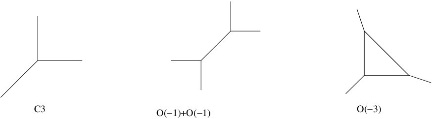
We let Tℝ≅U​(1)2T_{\mathbb{R}}\cong U(1)^{2} be the maximal compact subgroup of TT; let 𝔱ℝ{\mathfrak{t}}_{\mathbb{R}} and 𝔱ℝ∨\mathfrak{t}_{\mathbb{R}}^{\vee} be its Lie algebra and its dual; let μ:Y→𝔱ℝ∨\mu:Y\to{\mathfrak{t}}_{\mathbb{R}}^{\vee} be the moment map of the TℝT_{\mathbb{R}}-action on YY. Because of the canonical isomorphism 𝔱ℝ∨≅ΛT⊗ℤℝ{\mathfrak{t}}_{\mathbb{R}}^{\vee}\cong\Lambda_{T}\otimes_{\mathbb{Z}}\mathbb{R}, the image of Y1Y^{1} under μ\mu forms a planar trivalent graph Γ\Gamma in ℤ⊕2⊗ℤℝ\mathbb{Z}^{\oplus 2}\otimes_{\mathbb{Z}}\mathbb{R}. Some examples are shown in Figure 1.

Refer to caption
Figure 1.

The graph ΓY\Gamma_{Y} encodes the information of YY in that its edges and vertices correspond to irreducible components of Y1Y^{1} and fixed points Y0Y^{0}; the slope of an edge determines the TT-action on the corresponding component of Y1Y^{1}.

Let Y^\hat{Y} be the formal completion of YY along Y1Y^{1}. Then Y^\hat{Y} is a smooth formal Calabi-Yau scheme and inherits the TT-action on YY. The formal Calabi-Yau scheme Y^\hat{Y} together with the TT-action can be reconstructed from the graph ΓY\Gamma_{Y} (cf. (a) in Section 3.2 below). The construction of a relative FTCY threefold from a FTCY graph (given in Section 3.5) can be viewed as generalization of this reconstructing procedure.

3.2. Relative Toric Calabi-Yau Threefolds

A smooth relative toric Calabi-Yau threefold is a pair (Y,D)(Y,D) where YY is a smooth toric threefold, DD is a possibly disconnected, smooth (ℂ∗)3(\mathbb{C}^{*})^{3} invariant divisor of YY, such that the relative Calabi- Yau condition holds:

Λ3​ΩY​(log⁡D)≅𝒪Y.\Lambda^{3}\Omega_{Y}(\log D)\cong{\cal O}_{Y}.

A toric Calabi-Yau threefold can be viewed as a relative Calabi-Yau threefold where the divisor DD is empty.

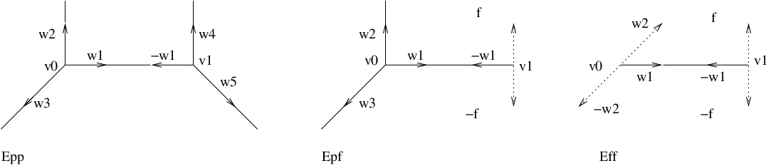
We now describe in details three examples of relative toric Calabi-Yau threefolds and their associated graphs, as they are the building blocks of the definitions and constructions in the rest of Section 3:

  1. (a)

    YY is the total space of 𝒪ℙ1​(−1+n)⊕𝒪ℙ1​(−1−n){\cal O}_{\mathbb{P}^{1}}(-1+n)\oplus{\cal O}_{\mathbb{P}^{1}}(-1-n).

  2. (b)

    YY is the total space of 𝒪ℙ1​(n)⊕𝒪ℙ1​(−1+n){\cal O}_{\mathbb{P}^{1}}(n)\oplus{\cal O}_{\mathbb{P}^{1}}(-1+n); DD is its fiber over q1=[1,0]∈ℙ1q_{1}=[1,0]\in{\mathbb{P}^{1}}.

  3. (c)

    YY is the total space of 𝒪ℙ1​(n)⊕𝒪ℙ1​(−n){\cal O}_{\mathbb{P}^{1}}(n)\oplus{\cal O}_{\mathbb{P}^{1}}(-n); DD is the union of its fibers over q0=[0,1]q_{0}=[0,1] and q1=[1,0]q_{1}=[1,0] in ℙ1{\mathbb{P}^{1}}.

Refer to caption
Figure 2.

In Figure 2, the edge connecting the two vertices v0v_{0} and v1v_{1} corresponds to the zero section ℙ1{\mathbb{P}^{1}}, which is a 1-dimensional (ℂ∗)3(\mathbb{C}^{*})^{3} orbit closure in YY; the vertices v0,v1v_{0},v_{1} correspond to the (ℂ∗)3(\mathbb{C}^{*})^{3} fixed points q0,q1∈ℙ1q_{0},q_{1}\in{\mathbb{P}^{1}}, respectively.

In Case (a), YY is a toric Calabi-Yau threefold, so we may specify a subtorus TT as in Section 3.1. The weights of the TT-action on the fibers of T​ℙ1,𝒪ℙ1​(−1+n),𝒪ℙ1​(−1−n)T{\mathbb{P}^{1}},{\cal O}_{\mathbb{P}^{1}}(-1+n),{\cal O}_{\mathbb{P}^{1}}(-1-n) at the TT-fixed point q0∈ℙ1q_{0}\in{\mathbb{P}^{1}} are given by w1,w2,w3∈ΛT≅ℤ⊕2w_{1},w_{2},w_{3}\in\Lambda_{T}\cong\mathbb{Z}^{\oplus 2}, respectively. We must have w1+w2+w3=0w_{1}+w_{2}+w_{3}=0 because TT acts on Λ3​Tq0​Y\Lambda^{3}T_{q_{0}}Y trivially. The weights of the TT-action on the fibers of T​ℙ1,𝒪ℙ1​(−1+n),𝒪ℙ1​(−1−n)T{\mathbb{P}^{1}},{\cal O}_{\mathbb{P}^{1}}(-1+n),{\cal O}_{\mathbb{P}^{1}}(-1-n) at the other fixed point q1∈ℙ1q_{1}\in{\mathbb{P}^{1}} are given by −w1,w2+(1−n)​w1,w3+(1+n)​w1=−w2+n​w1-w_{1},w_{2}+(1-n)w_{1},w_{3}+(1+n)w_{1}=-w_{2}+nw_{1}, respectively. From the graph in Figure 2(a), one can read off the degrees of the two summand of Nℙ1/YN_{{\mathbb{P}^{1}}/Y} and the TT-action on YY; YY together with the TT-action can be reconstructed from the graph.

Similarly, from the graph in Figure 2(b) (resp. (c)), one can reconstruct the pair (Y,D)(Y,D) in (b) (resp. (c)) together with the TT-action; the weights of the TT-action at fixed points can be read off from the graph as follows:

(b) T​ℙ1T{\mathbb{P}^{1}} 𝒪ℙ1​(n){\cal O}_{\mathbb{P}^{1}}(n) 𝒪ℙ1​(−1−n){\cal O}_{\mathbb{P}^{1}}(-1-n) (c) T​ℙ1T{\mathbb{P}^{1}} 𝒪ℙ1​(n){\cal O}_{\mathbb{P}^{1}}(n) 𝒪ℙ1​(−n){\cal O}_{\mathbb{P}^{1}}(-n)
q0q_{0} w1w_{1} w2w_{2} w3=−w1−w2w_{3}=-w_{1}-w_{2} q0q_{0} w1w_{1} w2w_{2} −w2-w_{2}
q1q_{1} −w1-w_{1} w2−n​w1w_{2}-nw_{1} w3+(1+n)​w1=−w2+n​w2\begin{array}[]{l}w_{3}+(1+n)w_{1}\\ =-w_{2}+nw_{2}\end{array} q1q_{1} −w1-w_{1} w2−n​w1w_{2}-nw_{1} −w2+n​w1-w_{2}+nw_{1}

3.3. FTCY Graphs

In this subsection, we will introduce formal toric Calabi-Yau (FTCY) graphs, which are graphs together with local embedding into ℝ2\mathbb{R}^{2} endowed with the standard orientation and integral lattice ℤ⊕2⊂ℝ2\mathbb{Z}^{\oplus 2}\subset\mathbb{R}^{2}.

As will be clear later, assigning a slope to an edge depends on the orientation of the edge. For book keeping purpose, we shall associate to each edge two (oppositely) oriented edges; for an oriented edge we can talk about its initial and terminal vertices. To recover the graph, we simply identify the two physically identical but oppositely oriented edges as one (unoriented) edge. This leads to the following definition.

Definition 3.1 (graphs).

A graph Γ\Gamma consists of a set of oriented edges Eo​(Γ)E^{\mathrm{o}}(\Gamma), a set of vertices V⁡(Γ)V(\Gamma), an orientation reversing map 𝔯​𝔢​𝔳:Eo​(Γ)→Eo​(Γ)\mathfrak{rev}\!:\!E^{\mathrm{o}}(\Gamma)\to E^{\mathrm{o}}(\Gamma), an initial vertex map 𝔳0:Eo​(Γ)→V⁡(Γ)\mathfrak{v}_{0}\!:\!E^{\mathrm{o}}(\Gamma)\to V(\Gamma) and a terminal vertex map 𝔳1:Eo​(Γ)→V⁡(Γ)\mathfrak{v}_{1}\!:\!E^{\mathrm{o}}(\Gamma)\to V(\Gamma), such that 𝔯​𝔢​𝔳\mathfrak{rev} is a fixed point free involution; that both 𝔳0\mathfrak{v}_{0} and 𝔳1\mathfrak{v}_{1} are surjective and 𝔳1=𝔳0∘𝔯​𝔢​𝔳\mathfrak{v}_{1}=\mathfrak{v}_{0}\circ\mathfrak{rev}. We say Γ\Gamma is weakly trivalent if |𝔳−1​(v)|≤3|\mathfrak{v}^{-1}(v)|\leq 3 for v∈V⁡(Γ)v\in V(\Gamma).

For simplicity, we will abbreviate 𝔯​𝔢​𝔳​(e)\mathfrak{rev}(e) to −e-e. Then the equivalence classes E⁡(Γ)=Eo​(Γ)/{±1}E(\Gamma)=E^{\mathrm{o}}(\Gamma)/\{\pm 1\} is the set of edges of Γ\Gamma in the ordinary sense. In case Γ\Gamma is weakly trivalent, we shall denote by V1​(Γ)V_{1}(\Gamma), V2​(Γ)V_{2}(\Gamma) and V3​(Γ)V_{3}(\Gamma) the sets of univalent, bivalent, and trivalent vertices of Γ\Gamma; we shall also define

E𝔣​(Γ)={e∈Eo​(Γ)∣𝔳1​(e)∈V1​(Γ)∪V2​(Γ)}E^{\mathfrak{f}}(\Gamma)=\{e\in E^{\mathrm{o}}(\Gamma)\mid\mathfrak{v}_{1}(e)\in V_{1}(\Gamma)\cup V_{2}(\Gamma)\}

which consists of oriented edges whose terminal edges are not trivalent. Finally, we fix a standard basis {u1,u2}\{u_{1},u_{2}\} of ℤ⊕2\mathbb{Z}^{\oplus 2} such that the ordered basis (u1,u2)(u_{1},u_{2}) determines the orientation on ℝ2\mathbb{R}^{2}.

Definition 3.2 (FTCY graphs).

A formal toric Calabi-Yau (FTCY) graph is a weakly trivalent graph Γ\Gamma together with a position map

𝔭:Eo​(Γ)⟶ℤ⊕2−{0}\mathfrak{p}:E^{\mathrm{o}}(\Gamma)\longrightarrow\mathbb{Z}^{\oplus 2}-\{0\}

and a framing map

𝔣:E𝔣​(Γ)⟶ℤ⊕2−{0},\mathfrak{f}:E^{\mathfrak{f}}(\Gamma)\longrightarrow\mathbb{Z}^{\oplus 2}-\{0\},

such that (see Figure 3)

  1. T1.

    𝔭\mathfrak{p} is anti-symmetric: 𝔭⁡(−e)=−𝔭⁡(e)\mathfrak{p}(-e)=-\mathfrak{p}(e).

  2. T2.

    𝔭\mathfrak{p} and 𝔣\mathfrak{f} are balanced:

    • •

      For a bivalent vertex v∈V2​(Γ)v\in V_{2}(\Gamma) with 𝔳1−1​(v)={e1,e2}\mathfrak{v}_{1}^{-1}(v)=\{e_{1},e_{2}\}, 𝔭⁡(e1)+𝔭⁡(e2)=0\mathfrak{p}(e_{1})+\mathfrak{p}(e_{2})=0 and 𝔣⁡(e1)+𝔣⁡(e2)=0\mathfrak{f}(e_{1})+\mathfrak{f}(e_{2})=0.

    • •

      For a trivalent v∈V3​(Γ)v\in V_{3}(\Gamma) with 𝔳0−1​(v)={e1,e2,e3}\mathfrak{v}_{0}^{-1}(v)=\{e_{1},e_{2},e_{3}\}, 𝔭⁡(e1)+𝔭⁡(e2)+𝔭⁡(e3)=0\mathfrak{p}(e_{1})+\mathfrak{p}(e_{2})+\mathfrak{p}(e_{3})=0.

  3. T3.

    𝔭\mathfrak{p} and 𝔣\mathfrak{f} are primitive:

    • •

      For a trivalent vertex v∈V3​(Γ)v\in V_{3}(\Gamma) with 𝔳0−1​(v)={e1,e2,e3}\mathfrak{v}_{0}^{-1}(v)=\{e_{1},e_{2},e_{3}\}, any two vectors in {𝔭⁡(e1),𝔭⁡(e2),𝔭⁡(e3)}\{\mathfrak{p}(e_{1}),\mathfrak{p}(e_{2}),\mathfrak{p}(e_{3})\} form an integral basis of ℤ⊕2\mathbb{Z}^{\oplus 2}

    • •

      For e∈E𝔣​(Γ)e\in E^{\mathfrak{f}}(\Gamma), 𝔭⁡(e)∧𝔣⁡(e)=u1∧u2\mathfrak{p}(e)\wedge\mathfrak{f}(e)=u_{1}\wedge u_{2}.

Refer to caption
Figure 3.

We say Γ\Gamma is a regular FTCY graph if it has no bivalent vertex.

The neighborhood of an oriented edge ee of an FTCY graph Γ\Gamma looks like (a), (b), or (c) in Figure 2 (if we add vectors {−𝔣⁡(e)∣𝔳1​(e)∈V1​(E)}\{-\mathfrak{f}(e)\mid\mathfrak{v}_{1}(e)\in V_{1}(E)\}). So to each edge we may associate a relative Calabi-Yau threefold (Ye,De)(Y^{e},D^{e}) where YeY^{e} is the total space of the direct sum of two line bundles over ℙ1{\mathbb{P}^{1}}. Since ee is oriented, we may assign LeL^{e}, one of the two line bundles, to ee as follows: in Figure 2(a), (b), or (c), if 𝔭⁡(e)=w1\mathfrak{p}(e)=w_{1} points to the right, so that v0v_{0} (resp. v1v_{1}) is the initial (resp. terminal) vertex of ee, then the weight of TT-action on Lq0eL^{e}_{q_{0}} (resp. Lq1eL^{e}_{q_{1}}) is given by the upward vector at v0v_{0} (resp. v1v_{1}), denoted by 𝔩0​(e)\mathfrak{l}_{0}(e) (resp. 𝔩1​(e)\mathfrak{l}_{1}(e)). Then YeY^{e} is the total space of Le⊕L−e→ℙ1L^{e}\oplus L^{-e}\to{\mathbb{P}^{1}}. This is the geometric interpretation of the following definition:

Definition 3.3.

Let Γ\Gamma be an FTCY graph. We define 𝔩0,𝔩1:Eo​(Γ)⟶ℤ⊕2\mathfrak{l}_{0},\mathfrak{l}_{1}:E^{\mathrm{o}}(\Gamma)\longrightarrow\mathbb{Z}^{\oplus 2} as follows:

𝔩0​(e)={−𝔣⁡(−e),𝔳0​(e)∉V3​(Γ),𝔭⁡(e01),𝔳0​(e)∈V3​(Γ).𝔩1​(e)={𝔣⁡(e),𝔳1​(e)∉V3​(Γ),𝔭⁡(e11),𝔳1​(e)∈V3​(Γ).\mathfrak{l}_{0}(e)=\begin{cases}-\mathfrak{f}(-e),&\mathfrak{v}_{0}(e)\notin V_{3}(\Gamma),\\ \mathfrak{p}(e_{01}),&\mathfrak{v}_{0}(e)\in V_{3}(\Gamma).\end{cases}\quad\quad\mathfrak{l}_{1}(e)=\begin{cases}\mathfrak{f}(e),&\mathfrak{v}_{1}(e)\notin V_{3}(\Gamma),\\ \mathfrak{p}(e_{11}),&\mathfrak{v}_{1}(e)\in V_{3}(\Gamma).\end{cases}

Here ei​1e_{i1} is the unique oriented edge such that 𝔳0​(ei​1)=𝔳i​(e)\mathfrak{v}_{0}(e_{i1})=\mathfrak{v}_{i}(e) and 𝔭⁡(e)∧𝔭⁡(ei​1)=u1∧u2\mathfrak{p}(e)\wedge\mathfrak{p}(e_{i1})=u_{1}\wedge u_{2}.

Refer to caption
Figure 4.

The degree of the line bundle LeL^{e} determines an integer nen^{e}:

(3.2) deg⁡Le={ne−1,v1∈V3​(Γ),ne,v1∉V3​(Γ).\deg L^{e}=\begin{cases}n^{e}-1,&v_{1}\in V_{3}(\Gamma),\\ n^{e},&v_{1}\notin V_{3}(\Gamma).\end{cases}

This motivates the following definition.

Definition 3.4.

We define n→:Eo​(Γ)→ℤ\vec{n}:E^{\mathrm{o}}(\Gamma)\to\mathbb{Z} by

𝔩1​(e)−𝔩0​(e)={(1−n→​(e))​𝔭​(e),𝔳1​(e)∈V3​(Γ),−n→​(e)​𝔭​(e),𝔳1​(e)∉V3​(Γ).\mathfrak{l}_{1}(e)-\mathfrak{l}_{0}(e)=\begin{cases}(1-\vec{n}(e))\mathfrak{p}(e),&\mathfrak{v}_{1}(e)\in V_{3}(\Gamma),\\ -\vec{n}(e)\mathfrak{p}(e),&\mathfrak{v}_{1}(e)\notin V_{3}(\Gamma).\end{cases}

We write nen^{e} for n→​(e)\vec{n}(e).

Note that n−e=−nen^{-e}=-n^{e}.

3.4. Operations on FTCY Graphs

In this subsection, we define four operations on FTCY graphs: smoothing, degeneration, normalization, and gluing. These operations extend natural operations on toric Calabi-Yau threefolds.

The first operation is the smoothing of a bivalent vertex v∈V2​(Γ)v\in V_{2}(\Gamma). In doing this, we shall eliminate the vertex vv and combine the two edges attached to vv.

Definition 3.5 (smoothing).

The smoothing of Γ\Gamma along a bivalent vertex v∈V2​(Γ)v\in V_{2}(\Gamma) is a graph Γv\Gamma_{v} that has vertices V⁡(Γ)−{v}V(\Gamma)-\{v\}, oriented edges Eo(Γ)/∼E^{\mathrm{o}}(\Gamma)/\sim with the equivalence ±e1∼∓e2\pm e_{1}\sim\mp e_{2} for {e1,e2}=𝔳1−1​(v)\{e_{1},e_{2}\}=\mathfrak{v}_{1}^{-1}(v). The maps 𝔳0\mathfrak{v}_{0}, 𝔳1\mathfrak{v}_{1}, 𝔭\mathfrak{p} and 𝔣\mathfrak{f} descends to corresponding maps on Γv\Gamma_{v}, making it a FTCY graph. ((See Figure 5: Γ3\Gamma_{3} is the smoothing of Γ2\Gamma_{2} along vv.))

The reverse of the above construction is called a degeneration.

Definition 3.6 (degeneration).

Let Γ\Gamma be a FTCY graph and let e∈Eo​(Γ)e\in E^{\mathrm{o}}(\Gamma) be an edge. We pick a lattice point 𝔣0∈ℤ⊕2\mathfrak{f}_{0}\in\mathbb{Z}^{\oplus 2} so that 𝔭⁡(e)∧𝔣0=u1∧u2\mathfrak{p}(e)\wedge\mathfrak{f}_{0}=u_{1}\wedge u_{2}. The degeneration of Γ\Gamma at ee with framing 𝔣0\mathfrak{f}_{0} is a graph Γe,𝔣o\Gamma_{e,\mathfrak{f}_{o}} whose edges are Eo​(Γ)∪{±e1,±e2}−{±e}E^{\mathrm{o}}(\Gamma)\cup\{\pm e_{1},\pm e_{2}\}-\{\pm e\} and whose vertices are V⁡(Γ)∪{v0}V(\Gamma)\cup\{v_{0}\}; its initial vertices 𝔳~0\tilde{\mathfrak{v}}_{0}, terminal vertices 𝔳~1\tilde{\mathfrak{v}}_{1}, position map 𝔭~\tilde{\mathfrak{p}} and framing map 𝔣~\tilde{\mathfrak{f}} are identical to those of Γ\Gamma except

𝔳~0​(e1)=𝔳0​(e),𝔳~1​(e1)=𝔳~1​(e2)=v0,𝔳~0​(e2)=𝔳1​(e),\displaystyle\tilde{\mathfrak{v}}_{0}(e_{1})=\mathfrak{v}_{0}(e),\ \tilde{\mathfrak{v}}_{1}(e_{1})=\tilde{\mathfrak{v}}_{1}(e_{2})=v_{0},\ \tilde{\mathfrak{v}}_{0}(e_{2})=\mathfrak{v}_{1}(e),
𝔭~​(e1)=−𝔭~​(e2)=𝔭⁡(e),𝔣~​(e1)=𝔣~​(e2)=𝔣0.\displaystyle\tilde{\mathfrak{p}}(e_{1})=-\tilde{\mathfrak{p}}(e_{2})=\mathfrak{p}(e),\ \tilde{\mathfrak{f}}(e_{1})=\tilde{\mathfrak{f}}(e_{2})=\mathfrak{f}_{0}.

((See Figure 5: Γ2\Gamma_{2} is the degeneration of Γ3\Gamma_{3} at ee with framing 𝔣0\mathfrak{f}_{0}.))

The normalization is to separate a graph along a bivalent vertex and the gluing is its inverse.

Definition 3.7 (normalization).

Let Γ\Gamma be a FTCY graph and let v∈V2​(Γ)v\in V_{2}(\Gamma) be a bivalent vertex. The normalization of Γ\Gamma at vv is a graph Γv\Gamma^{v} whose edges are the same as that of Γ\Gamma and whose vertices are V⁡(Γ)∪{v1,v2}−{v}V(\Gamma)\cup\{v_{1},v_{2}\}-\{v\}; its associated maps 𝔳~0\tilde{\mathfrak{v}}_{0}, 𝔳~1\tilde{\mathfrak{v}}_{1}, 𝔭~\tilde{\mathfrak{p}} and 𝔣~\tilde{\mathfrak{f}} are identical to that of Γ\Gamma except for {e1,e2}=𝔳1−1​(v)\{e_{1},e_{2}\}=\mathfrak{v}_{1}^{-1}(v), 𝔳~1​(e1)=v1\tilde{\mathfrak{v}}_{1}(e_{1})=v_{1} and 𝔳~1​(e2)=v2\tilde{\mathfrak{v}}_{1}(e_{2})=v_{2}. ((See Figure 5: Γ1\Gamma_{1} is the normalization of Γ2\Gamma_{2} at vv.))

Definition 3.8 (gluing).

Let Γ\Gamma be a FTCY graph and let v1,v2∈V1​(Γ)v_{1},v_{2}\in V_{1}(\Gamma) be two univalent vertices of Γ\Gamma. Let 𝔣i=𝔣⁡(ei)\mathfrak{f}_{i}=\mathfrak{f}(e_{i}), where {ei}=𝔳1−1​(vi)\{e_{i}\}=\mathfrak{v}_{1}^{-1}(v_{i}). Suppose 𝔭⁡(e1)=−𝔭⁡(e2)\mathfrak{p}(e_{1})=-\mathfrak{p}(e_{2}) and 𝔣1=−𝔣2\mathfrak{f}_{1}=-\mathfrak{f}_{2}. We then identify v1v_{1} and v2v_{2} to form a single vertex, and keep the framing 𝔣⁡(ei)=𝔣i\mathfrak{f}(e_{i})=\mathfrak{f}_{i}. The resulting graph Γv1,v2\Gamma^{v_{1},v_{2}} is called the gluing of Γ\Gamma at v1v_{1} and v2v_{2}. ((See Figure 5: Γ2\Gamma_{2} is the gluing of Γ1\Gamma_{1} at v1v_{1} and v2v_{2}.))

Refer to caption
Figure 5.

It is straightforward to generalize smoothing and normalization to subset AA of V2​(Γ)V_{2}(\Gamma). Given A⊂V2​(Γ)A\subset V_{2}(\Gamma), let ΓA\Gamma_{A} denote the smoothing of Γ\Gamma along AA, and let ΓA\Gamma^{A} denote the normalization of Γ\Gamma along AA. There are surjective maps

πA:E⁡(Γ)→E⁡(ΓA),πA:V⁡(ΓA)→V⁡(Γ).\pi_{A}:E(\Gamma)\to E(\Gamma_{A}),\quad\pi^{A}:V(\Gamma^{A})\to V(\Gamma).

3.5. Relative FTCY Threefolds

In this subsection we will introduce relative formal toric Calabi-Yau (FTCY) threefolds.

Given a FTCY graph Γ\Gamma, we will construct a pair Y^rel=(Y^,D^)\hat{Y}^{\mathrm{rel}}=(\hat{Y},\hat{D}), where Y^\hat{Y} is a threefold, possibly with normal crossing singularities, D^⊂Y^\hat{D}\subset\hat{Y} is a relative divisor, so that Y^rel=(Y^,D^)\hat{Y}^{\mathrm{rel}}=(\hat{Y},\hat{D}) is a formal relative Calabi-Yau threefold:

(3.3) ∧3ΩY^(logD^)≅𝒪Y^.\wedge^{3}\Omega_{\hat{Y}}(\log\hat{D})\cong{\cal O}_{\hat{Y}}.

The pair (Y^,D^)(\hat{Y},\hat{D}) admits a TT-action so that the action on Λ3​Tp​Y^\Lambda^{3}T_{p}\hat{Y} is trivial for any fixed point pp. As a set, the scheme Y^\hat{Y} is a union of ℙ1{\mathbb{P}^{1}}’s, each associated to an edge of Γ\Gamma; two ℙ1{\mathbb{P}^{1}} intersect exactly when their associated edges share a common vertex; the normal bundle to each ℙ1{\mathbb{P}^{1}} in Y^\hat{Y} and the TT-action on Y^\hat{Y} are dictated by the data encoded in the graph Γ\Gamma. We will also specify a TT-invariant divisor L^⊂D^\hat{L}\subset\hat{D}.

In the following construction, we will use the notation introduced in Section 3.3.

3.5.1. Edges

Let e∈Eo​(Γ)e\in E^{\mathrm{o}}(\Gamma) with v0v_{0} and v1v_{1} its initial and terminal vertices. We let TT acts on ℙ1{\mathbb{P}^{1}} by

t⋅[X,Y]=[𝔭⁡(e)​(t)​X,Y],t∈T.t\cdot[X,Y]=[\mathfrak{p}(e)(t)X,Y],\quad t\in T.

Here we view 𝔭⁡(e)\mathfrak{p}(e) as an element in ΛT=Hom⁡(T,ℂ∗)\Lambda_{T}=\Hom(T,\mathbb{C}^{*}). We denote the two fixed points by q0=[0,1]q_{0}=[0,1] and q1=[1,0]q_{1}=[1,0]. Next we let Le→ℙ1L^{e}\to{\mathbb{P}^{1}} be the line bundle of

deg⁡Le={ne−1,v1∈V3​(Γ),ne,v1∉V3​(Γ),\deg L^{e}=\begin{cases}n^{e}-1,&v_{1}\in V_{3}(\Gamma),\\ n^{e},&v_{1}\notin V_{3}(\Gamma),\end{cases}

where ne=n→​(e)n^{e}=\vec{n}(e) is defined in Definition 3.4. We let L−eL^{-e} be the line bundle on ℙ1{\mathbb{P}^{1}} of degree n−e−1n^{-e}-1 (resp. n−en^{-e}) when v0v_{0} is trivalent (resp. non-trivalent). We then assign the TT-action at Lq0eL^{e}_{q_{0}} be 𝔩0​(e)\mathfrak{l}_{0}(e) and at Lq1eL^{e}_{q_{1}} be 𝔩1​(e)\mathfrak{l}_{1}(e); assign the TT-action at Lq1−eL^{-e}_{q_{1}} be 𝔩0​(−e)\mathfrak{l}_{0}(-e) and at Lq0−eL^{-e}_{q_{0}} be 𝔩1​(−e)\mathfrak{l}_{1}(-e) (see Figures 4).

Next, we let Σ⁡(e)\Sigma(e) be the formal completion of the total space of Le⊕L−eL^{e}\oplus L^{-e} along its zero section. The TT-actions on LeL^{e} and on L−eL^{-e} induce a TT-action on Σ⁡(e)\Sigma(e). By construction, there is a TT-isomorphism

(3.4) Σ⁡(e)≅Σ⁡(−e)\Sigma(e)\cong\Sigma(-e)

that sends [0,1]∈Σ⁡(e)[0,1]\in\Sigma(e) to [1,0]∈Σ⁡(−e)[1,0]\in\Sigma(-e) and sends the first summand LeL^{e} in Nℙ1/Σ⁡(e)N_{{\mathbb{P}^{1}}/\Sigma(e)} to the second summand LeL^{e} in Nℙ1/Σ⁡(−e)N_{{\mathbb{P}^{1}}/\Sigma(-e)}.

It is clear that

(3.5) ∧3ΩΣ⁡(e)≅p∗𝒪ℙ1(c),\wedge^{3}\Omega_{\Sigma(e)}\cong p^{*}{\cal O}_{{\mathbb{P}^{1}}}(c),

where p:Σ⁡(e)→ℙ1p\!:\!\Sigma(e)\to{\mathbb{P}^{1}} is the projection, and c=#⁡({v0,v1}∩V3​(Γ))−2c=\#(\{v_{0},v_{1}\}\cap V_{3}(\Gamma))-2.

3.5.2. Gluing along Trivalent Vertices

Given v∈V3​(Γ)v\in V_{3}(\Gamma) with 𝔳0−1​(v)={e1,e2,e3}\mathfrak{v}_{0}^{-1}(v)=\{e_{1},e_{2},e_{3}\} so indexed so that 𝔭⁡(e1),𝔭⁡(e2),𝔭⁡(e3)\mathfrak{p}(e_{1}),\mathfrak{p}(e_{2}),\mathfrak{p}(e_{3}) is in counter-clockwise order.

To glue the formal scheme Σ⁡(e1)\Sigma(e_{1}), Σ⁡(e2)\Sigma(e_{2}) and Σ⁡(e3)\Sigma(e_{3}), we introduce a TT-scheme

Σ⁡(v)=Spec⁡ℂ⁡[[x1,x2,x3]],with T-action​t⋅xi=𝔭⁡(ei)​(t)​xi∀t∈T,\Sigma(v)=\spec\mathbb{C}[\![x_{1},x_{2},x_{3}]\!],\quad\text{with $T$-action}\ t\cdot x_{i}=\mathfrak{p}(e_{i})(t)x_{i}\quad\forall\ t\in T,

and gluing morphisms

(3.6) ψek​v:Σ⁡(v)⟶Σ⁡(ek)\psi_{e_{k}v}:\Sigma(v)\longrightarrow\Sigma(e_{k})

according to the following rule. First, we let Σ^​(ek)\hat{\Sigma}(e_{k}) be the formal completion of Σ⁡(ek)\Sigma(e_{k}) along q0∈ℙ1⊂Σ⁡(ek)q_{0}\in{\mathbb{P}^{1}}\subset\Sigma(e_{k}). Σ^​(ek)\hat{\Sigma}(e_{k}) is a formal TT-scheme and is TT-isomorphic to the TT-scheme

Spec⁡ℂ⁡[[y1,y2,y3]];t⋅yi=𝔭⁡(ei+k)​(t)​yi\spec\mathbb{C}[\![y_{1},y_{2},y_{3}]\!];\quad t\cdot y_{i}=\mathfrak{p}(e_{i+k})(t)y_{i}
22 2 Here we agree that ek+3=eke_{k+3}=e_{k}; same for xi+3=xix_{i+3}=x_{i} later.

such that Lq0ekL^{e_{k}}_{q_{0}}, Lq1−ekL^{-e_{k}}_{q_{1}}, Tq0​ℙ1T_{q_{0}}\mathbb{P}^{1} are mapped to ℂ​∂∂y1\mathbb{C}\frac{\partial}{\partial y_{1}}, ℂ​∂∂y2\mathbb{C}\frac{\partial}{\partial y_{2}}, ℂ​∂∂y3\mathbb{C}\frac{\partial}{\partial y_{3}}, respectively. The gluing morphism ψek​v\psi_{e_{k}v} is the composite of

(3.7) Spec⁡ℂ⁡[[y1,y2,y3]]⟶Σ^​(ek)⟶Σ⁡(ek)\spec\mathbb{C}[\![y_{1},y_{2},y_{3}]\!]\longrightarrow\hat{\Sigma}(e_{k})\longrightarrow\Sigma(e_{k})

with the TT-isomorphism

Σ⁡(v)≡Spec⁡ℂ⁡[[x1,x2,x3]]⟶Spec⁡ℂ⁡[[y1,y2,y3]]\Sigma(v)\equiv\spec\mathbb{C}[\![x_{1},x_{2},x_{3}]\!]\longrightarrow\spec\mathbb{C}[\![y_{1},y_{2},y_{3}]\!]

defined by yi↦xk+iy_{i}\mapsto x_{k+i}.

Using the morphisms ψek​v\psi_{e_{k}v}, we can glue Σ⁡(e1)\Sigma(e_{1}) and Σ⁡(e2)\Sigma(e_{2}) and then glue Σ⁡(e3)\Sigma(e_{3}) onto it via the cofiber products

Σ⁡(e1)→Σ⁡(e1)​∐Σ⁡(v)Σ⁡(e2)↑↑Σ⁡(v)→Σ⁡(e2)Σ⁡(e3)→Σ⁡(e1)​∐Σ⁡(v)Σ⁡(e2)​∐Σ⁡(v)Σ⁡(e3)↑↑Σ⁡(v)→Σ⁡(e1)​∐Σ⁡(v)Σ⁡(e2)\begin{CD}\Sigma(e_{1})@>{}>{}>\Sigma(e_{1})\coprod_{\Sigma(v)}\Sigma(e_{2})\\ @A{}A{}A@A{}A{}A\\ \Sigma(v)@>{}>{}>\Sigma(e_{2})\end{CD}\qquad\begin{CD}\Sigma(e_{3})@>{}>{}>\Sigma(e_{1})\coprod_{\Sigma(v)}\Sigma(e_{2})\coprod_{\Sigma(v)}\Sigma(e_{3})\\ @A{}A{}A@A{}A{}A\\ \Sigma(v)@>{}>{}>\Sigma(e_{1})\coprod_{\Sigma(v)}\Sigma(e_{2})\end{CD}

Since the gluing map ψek​v\psi_{e_{k}v} are TT-equivalent, the TT-actions on Σ⁡(ek)\Sigma(e_{k}) descend to the glued scheme.

3.5.3. Gluing along Bivalent Vertices

Next we glue Σ⁡(e1)\Sigma(e_{1}) and Σ⁡(e2)\Sigma(e_{2}) in case {e1,e2}=𝔳0−1​(v)\{e_{1},e_{2}\}=\mathfrak{v}_{0}^{-1}(v) for a v∈V2​(Γ)v\in V_{2}(\Gamma). Note that 𝔩0​(e1)+𝔩0​(e2)=0\mathfrak{l}_{0}(e_{1})+\mathfrak{l}_{0}(e_{2})=0. Let Σ⁡(v)\Sigma(v) be the formal TT-scheme

Σ⁡(v)=Spec⁡ℂ⁡[[x1,x2]],t⋅xi=𝔩0​(ei)​(t)​xi;\Sigma(v)=\spec\mathbb{C}[\![x_{1},x_{2}]\!],\quad t\cdot x_{i}=\mathfrak{l}_{0}(e_{i})(t)x_{i};

we let the gluing morphism ψek​v\psi_{e_{k}v} of (3.6) be the composite of (3.7) with the TT-morphism

Spec⁡ℂ⁡[[x1,x2]]⟶Spec⁡ℂ⁡[[y1,y2,y3]]\spec\mathbb{C}[\![x_{1},x_{2}]\!]\longrightarrow\spec\mathbb{C}[\![y_{1},y_{2},y_{3}]\!]

defined via y3↦0y_{3}\mapsto 0, y1y_{1} and y2y_{2} map to x1x_{1} and x2x_{2} respectively in case k=1k=1 and to x2x_{2} and x1x_{1} respectively in case k=2k=2. We can glue Σ⁡(e1)\Sigma(e_{1}) and Σ⁡(e2)\Sigma(e_{2}) along Σ⁡(v)\Sigma(v) via the cofiber product as before.

3.5.4. Univalent vertices

Lastly, we consider the case e1=𝔳0−1​(v)e_{1}=\mathfrak{v}_{0}^{-1}(v) for a v∈V1​(Γ)v\in V_{1}(\Gamma). Note that 𝔩0​(e)+𝔩1​(−e)=0\mathfrak{l}_{0}(e)+\mathfrak{l}_{1}(-e)=0. Let Σ⁡(v)\Sigma(v) be the formal TT-scheme

Σ⁡(v)=Spec⁡ℂ⁡[[x1,x2]],t⋅x1=𝔩0​(e1)​(t)​x1,t⋅x2=𝔩1​(−e1)​(t)​x2;\Sigma(v)=\spec\mathbb{C}[\![x_{1},x_{2}]\!],\quad t\cdot x_{1}=\mathfrak{l}_{0}(e_{1})(t)x_{1},\quad t\cdot x_{2}=\mathfrak{l}_{1}(-e_{1})(t)x_{2};

and define ψe1​v\psi_{e_{1}v} in (3.6). We let D^v\hat{D}^{v} be the image divisor ψe1​v​(Σ⁡(v))⊂Σ⁡(e1)\psi_{e_{1}v}(\Sigma(v))\subset\Sigma(e_{1}) and consider it as part of the relative divisor of the formal Calabi-Yau scheme Y^rel\hat{Y}^{\mathrm{rel}} we are constructing.

Let L⁡(v)⊂Σ⁡(v)L(v)\subset\Sigma(v) be the divisor defined by x2=0x_{2}=0, and let L^v=ψe1​v​(L⁡(v))⊂D^v\hat{L}^{v}=\psi_{e_{1}v}(L(v))\subset\hat{D}^{v}.

3.5.5. Final step

Now it is standard to glue all Σ⁡(e)\Sigma(e) to form a scheme Y^\hat{Y}. We first form the disjoint union

∐e∈Eo​(Γ)Σ⁡(e);\coprod_{e\in E^{\mathrm{o}}(\Gamma)}\Sigma(e);

because of (3.4), the orientation reversing map Eo​(Γ)→Eo​(Γ)E^{\mathrm{o}}(\Gamma)\to E^{\mathrm{o}}(\Gamma) defines a fixed point free involution

τ:∐e∈Eo​(Γ)Σ⁡(e)⟶∐e∈Eo​(Γ)Σ⁡(e);\tau:\coprod_{e\in E^{\mathrm{o}}(\Gamma)}\Sigma(e)\longrightarrow\coprod_{e\in E^{\mathrm{o}}(\Gamma)}\Sigma(e);

we define Y~\tilde{Y} be its quotient by τ\tau. Next, for each trivalent vertex vv with 𝔳0−1​(v)={e1,e2,e3}\mathfrak{v}_{0}^{-1}(v)=\{e_{1},e_{2},e_{3}\}, we glue Σ⁡(e1),Σ⁡(e2),Σ⁡(e3)\Sigma(e_{1}),\Sigma(e_{2}),\Sigma(e_{3}) along Σ⁡(v)\Sigma(v); for each bivalent vertex vv with 𝔳0−1​(v)={e1,e2}\mathfrak{v}_{0}^{-1}(v)=\{e_{1},e_{2}\}, we glue Σ⁡(e1)\Sigma(e_{1}) and Σ⁡(e2)\Sigma(e_{2}) along Σ⁡(v)\Sigma(v). We denote by Y^\hat{Y} the resulting scheme after completing all the gluing associated to all trivalent and bivalent vertices. The TT-action on Σ⁡(e)\Sigma(e)’s descends to a TT-action on Y^\hat{Y}. Finally, for each univalent vertex vv with e=𝔳0−1​(v)e=\mathfrak{v}_{0}^{-1}(v), we let D^v⊂Σ⁡(e)\hat{D}^{v}\subset\Sigma(e) be the divisor defined in Section 3.5.4. The (disjoint) union of all such D^v\hat{D}^{v} form a divisor D^\hat{D} that is the relative divisor of Y^\hat{Y}. Since D^\hat{D} is invariant under TT, the pair Y^rel=(Y^,D^)\hat{Y}^{\mathrm{rel}}=(\hat{Y},\hat{D}) is a TT-equivariant formal scheme. Because of (3.5), we have

∧3ΩY^(logD^)≅𝒪Y^;\wedge^{3}\Omega_{\hat{Y}}(\log\hat{D})\cong{\cal O}_{\hat{Y}};

hence Y^rel=(Y^,D^)\hat{Y}^{\mathrm{rel}}=(\hat{Y},\hat{D}) is a formal toric Calabi-Yau scheme.

Following the construction, the scheme Y^\hat{Y} is smooth away from the images ψe​v​(Σ​(v))\psi_{ev}(\Sigma(v)) associated to bivalent vertices vv, and has normal crossing singularities there. Therefore Y^\hat{Y} is smooth when Γ\Gamma has no bivalent vertices. The relative divisor D^\hat{D} is the union of smooth divisor D^v\hat{D}^{v} indexed by v∈V1​(Γ)v\in V_{1}(\Gamma). Within each divisor D^v\hat{D}^{v} there is a divisor L^v⊂D^v\hat{L}^{v}\subset\hat{D}^{v} defined as in Section 3.5.4.

For later convenience, we introduce some notation. Let e¯{\bar{e}} denote the equivalence class {e,−e}\{e,-e\} in E⁡(Γ)E(\Gamma), and let Ce¯C^{\bar{e}} denote the projective line in Y^\hat{Y} coming from the ℙ1{\mathbb{P}^{1}} in Σ⁡(e)\Sigma(e). For v∈V1​(Γ)v\in V_{1}(\Gamma), let zvz^{v} denote the point in D^v\hat{D}^{v} coming from the closed point q0q_{0} in Σ⁡(e)\Sigma(e), where 𝔳0​(e)=v\mathfrak{v}_{0}(e)=v.

4. Definition of Formal Relative Gromov-Witten Invariants

In this section, we will define relative Gromov-Witten invariants of relative FTCY threefolds; the case when the relative FTCY threefold is indecomposable gives the mathematical definition of topological vertex.

4.1. Moduli Spaces of Relative Stable morphisms

Let Γ\Gamma be a FTCY graph and let Y^rel=(Y^,D^)\hat{Y}^{\mathrm{rel}}=(\hat{Y},\hat{D}) be its associated scheme. Clearly, the degrees and the ramification patterns of relative stable morphisms to Y^rel\hat{Y}^{\mathrm{rel}} are characterized by effective classes of Γ\Gamma:

Definition 4.1 (effective class).

Let Γ\Gamma be a FTCY graph. An effective class of Γ\Gamma is a pair of functions d→:E⁡(Γ)→ℤ≥0\vec{d}\!:\!E(\Gamma)\to\mathbb{Z}_{\geq 0} and μ→:V1​(Γ)→𝒫{\vec{\mu}}\!:\!V_{1}(\Gamma)\to{\cal P} that satisfy

  1. (1)

    |μ→​(v)|=d→​(e¯)|{\vec{\mu}}(v)|=\vec{d}({\bar{e}}) if v∈V1​(Γ)v\in V_{1}(\Gamma) and 𝔳1​(e)=v\mathfrak{v}_{1}(e)=v;

  2. (2)

    d→​(e¯1)=d→​(e¯2)\vec{d}({\bar{e}}_{1})=\vec{d}({\bar{e}}_{2}) if v∈V2​(Γ)v\in V_{2}(\Gamma) and 𝔳0−1​(v)={e1,e2}\mathfrak{v}_{0}^{-1}(v)=\{e_{1},e_{2}\}.

We write μv\mu^{v} for μ→​(v){\vec{\mu}}(v), de¯d^{\bar{e}} for d→​(e¯)\vec{d}({\bar{e}}).

To show that an effective class does characterize a relative stable morphism, a quick review of its definition is in order. An ordinary relative morphism uu to (Y^,D^)(\hat{Y},\hat{D}) consists of

  • •

    a possibly disconnected nodal curve XX

  • •

    distinct smooth points {qjv∣v∈V0(Γ),1≤j≤ℓ(μv)}\{q_{j}^{v}\mid v\in V_{0}(\Gamma),1\leq j\leq\ell(\mu^{v})\} in XX such that each connected component of X contains at least one of these points,

  • •

    a morphism u:X→Y^u\!:\!X\to\hat{Y}

so that

  • •

    u−1​(D^v)=∑j=1ℓ⁡(μv)μjv​qjvu^{-1}(\hat{D}^{v})=\sum_{j=1}^{\ell(\mu^{v})}\mu_{j}^{v}q_{j}^{v} for some positive integers μjv\mu_{j}^{v};

  • •

    uu is pre-deformable along the singular loci

    ∐v∈V2​(Γ)Σ⁡(v)\coprod_{v\in V_{2}(\Gamma)}\Sigma(v)

    of Y^rel\hat{Y}^{\mathrm{rel}}, i.e, if v∈V2​(Γ)v\in V_{2}(\Gamma) and 𝔳0−1​(v)={e1,e2}\mathfrak{v}_{0}^{-1}(v)=\{e_{1},e_{2}\} , then u−1​(Σ​(v))u^{-1}(\Sigma(v)) consists of nodes of XX, and for each y∈u−1​(Σ​(v))y\in u^{-1}(\Sigma(v)), u|u−1​(Σ⁡(e1))u|_{u^{-1}(\Sigma(e_{1}))} and u|u−1​(Σ⁡(e2))u|_{u^{-1}(\Sigma(e_{2}))} have the same contact order to Σ⁡(v)\Sigma(v) at yy;

  • •

    uu coupled with the marked points qivq_{i}^{v} is a stable morphism in the ordinary sense.

Unless otherwise specified, all the stable morphisms in this paper are with not necessarily connected domain.

Since

H2​(Y^,ℤ)=⨁e¯∈E⁡(Γ)ℤ⁡[Ce¯],H_{2}(\hat{Y};\mathbb{Z})=\bigoplus_{{\bar{e}}\in E(\Gamma)}\mathbb{Z}[C^{\bar{e}}],

the morphism uu defines a map d→:E⁡(Γ)→ℤ\vec{d}\!:\!E(\Gamma)\to\mathbb{Z} via

(4.1) u∗​([X])=∑e¯∈E⁡(Γ)d→​(e¯)​[Ce¯].u_{\ast}([X])=\sum_{{\bar{e}}\in E(\Gamma)}\vec{d}({\bar{e}})[C^{\bar{e}}].

The integers μjv\mu_{j}^{v} form a partition

μv=(μ1v,⋯,μℓ⁡(μv)v)\mu^{v}=(\mu^{v}_{1},\cdots,\mu^{v}_{\ell(\mu^{v})})

and the map μ→:V1​(Γ)→𝒫{\vec{\mu}}\!:\!V_{1}(\Gamma)\to{\cal P} is

μ→​(v)=μv.{\vec{\mu}}(v)=\mu^{v}.

With this definition, the requirement (1) in Definition 4.1 follows from (4.1) and (2) holds since uu is pre-deformable.

To define relative stable morphisms to Y^rel\hat{Y}^{\mathrm{rel}}, we need to work with the expanded schemes of Y^rel\hat{Y}^{\mathrm{rel}} introduced in [24]. In the case studied, they are the associated formal schemes of the expanded graphs of Γ\Gamma.

Definition 4.2.

Let Γ\Gamma be a FTCY graph. A flat chain of length nn in Γ\Gamma is a subgraph Γˇ⊂Γ\check{\Gamma}\subset\Gamma that has nn edges ±e1,⋯,±en\pm e_{1},\cdots,\pm e_{n}, n+1n+1 univalent or bivalent vertices v0,⋯,vnv_{0},\cdots,v_{n} with identical framings 𝔣\mathfrak{f} (up to sign) so that

𝔳0(e1)=v0;𝔳1(ei)=𝔳0(ei+1)=vii=1,⋯,n−1;𝔳1(en)=vn,\mathfrak{v}_{0}(e_{1})=v_{0};\quad\mathfrak{v}_{1}(e_{i})=\mathfrak{v}_{0}(e_{i+1})=v_{i}\ i=1,\cdots,n-1;\quad\mathfrak{v}_{1}(e_{n})=v_{n},

and that all 𝔭⁡(ei)\mathfrak{p}(e_{i}) are identical.

Refer to caption
Figure 6. A flat chain of length nn
Definition 4.3.

A contraction of a FTCY graph Γ\Gamma along a flat chain Γˇ⊂Γ\check{\Gamma}\subset\Gamma is the graph after eliminating all edges and bivalent vertices of Γˇ\check{\Gamma} from Γ\Gamma, identifying the univalent vertices of Γˇ\check{\Gamma} while keeping their framings unchanged.

Given a FTCY graph Γ\Gamma and a function

𝐦:V1​(Γ)∪V2​(Γ)⟶ℤ≥0,\mathbf{m}:V_{1}(\Gamma)\cup V_{2}(\Gamma)\longrightarrow\mathbb{Z}_{\geq 0},

the expanded graph Γ𝐦\Gamma_{\mathbf{m}} is obtained by replacing each v∈V1​(Γ)∪V2​(Γ)v\in V_{1}(\Gamma)\cup V_{2}(\Gamma) by a flat chain Γˇmvv\check{\Gamma}^{v}_{m^{v}} of length mv=𝐦⁡(v)m^{v}=\mathbf{m}(v) with framings ±𝔣⁡(e)\pm\mathfrak{f}(e), where 𝔳1​(e)=v\mathfrak{v}_{1}(e)=v. In particular Γ𝟎=Γ\Gamma_{\mathbf{0}}=\Gamma, where 𝟎​(v)=0\mathbf{0}(v)=0 for all v∈V1​(Γ)∪V2​(Γ)v\in V_{1}(\Gamma)\cup V_{2}(\Gamma). The original graph Γ\Gamma can be recovered by contracting Γ𝐦\Gamma_{\mathbf{m}} along the flat chains

{Γˇmvv∣v∈V1​(Γ)∪V2​(Γ)}.\{\check{\Gamma}^{v}_{m^{v}}\mid v\in V_{1}(\Gamma)\cup V_{2}(\Gamma)\}.

We now study their associated Calabi-Yau scheme. We denote by (Y^,D^)(\hat{Y},\hat{D}) the associated Calabi-Yau scheme of Γ\Gamma and by (Y^𝐦,D^𝐦)(\hat{Y}_{\mathbf{m}},\hat{D}_{\mathbf{m}}) that of Γ𝐦\Gamma_{\mathbf{m}}. We recover the original scheme Y^\hat{Y} by shrinking the irreducible components of Y^𝐦\hat{Y}_{\mathbf{m}} associated to the flat chains that are contracted. This way we define a projection

π𝐦:Y^𝐦⟶Y^.\pi_{\mathbf{m}}:\hat{Y}_{\mathbf{m}}\longrightarrow\hat{Y}.

We define a relative automorphism of Y^𝐦\hat{Y}_{\mathbf{m}} to be an automorphism of Y^𝐦\hat{Y}_{\mathbf{m}} that is also a Y^\hat{Y}-morphism; an automorphism of a relative morphism u:X→(Y^𝐦,D^𝐦)u\!:\!X\to(\hat{Y}_{\mathbf{m}},\hat{D}_{\mathbf{m}}) is a pair of a relative automorphism σ\sigma of Y^𝐦\hat{Y}_{\mathbf{m}} and an automorphism hh of XX so that

u∘h=σ∘u.u\circ h=\sigma\circ u.
Definition 4.4.

A relative morphism to Y^Γrel\hat{Y}_{\Gamma}^{\mathrm{rel}} is an ordinary relative morphism to (Y^𝐦,D^𝐦)(\hat{Y}_{\mathbf{m}},\hat{D}_{\mathbf{m}}) for some 𝐦\mathbf{m}; it is stable if its automorphism group is finite.

Note that an effective class (d→,μ→)(\vec{d},{\vec{\mu}}) of an FTCY graph Γ\Gamma can also be viewed as an effective class of any degeneration of Γ\Gamma, and in particular, an effective class of Γ𝐦\Gamma_{\mathbf{m}}. We fix a FTCY graph Γ\Gamma, an effective class (d→,μ→)(\vec{d},{\vec{\mu}}), and an even integer χ\chi. We then form the moduli space ℳχ,d→,μ→∙​(Y^rel){\cal M}^{\bullet}_{\chi,\vec{d},{\vec{\mu}}}(\hat{Y}^{\mathrm{rel}}) of all stable relative morphisms uu to Y^rel\hat{Y}^{\mathrm{rel}} that satisfy

  • •

    χ⁡(𝒪X)=χ/2\chi({\cal O}_{X})=\chi/2, where XX is the domain curve of uu;

  • •

    the associated effective class of uu is (d→,μ→)(\vec{d},{\vec{\mu}}).

Since Y^\hat{Y} is a formal Calabi-Yau threefold with possibly normal crossing singularity and smooth singular loci, the moduli space ℳχ,d→,μ→∙​(Y^rel){\cal M}^{\bullet}_{\chi,\vec{d},{\vec{\mu}}}(\hat{Y}^{\mathrm{rel}}) is a formal Deligne-Mumford stack with a perfect obstruction theory [24, 25].

Lemma 4.5.

The virtual dimension of ℳχ,d→,μ→∙​(Y^rel){\cal M}^{\bullet}_{\chi,\vec{d},{\vec{\mu}}}(\hat{Y}^{\mathrm{rel}}) is ∑v∈V1​(Γ)ℓ⁡(μv)\sum_{v\in V_{1}(\Gamma)}\ell(\mu^{v}).

Proof.

The proof is straightforward and will be omitted. ∎

4.2. Equivariant Degeneration

Let TT act on ℙ1×𝔸1{\mathbb{P}^{1}}\times{\mathbb{A}}^{\!1} by

t⋅([X0,X1],s)=([𝔭⁡(t)​X0,X1],s),t\cdot([X_{0},X_{1}],s)=([\mathfrak{p}(t)X_{0},X_{1}],s),

where 𝔭∈ΛT=Hom⁡(T,ℂ∗)\mathfrak{p}\in\Lambda_{T}=\Hom(T,\mathbb{C}^{*}). Let 𝔜\mathfrak{Y} be the blowup of ℙ1×𝔸1{\mathbb{P}^{1}}\times{\mathbb{A}}^{\!1} at ([0,1],0)([0,1],0). The TT-action on ℙ1×𝔸1{\mathbb{P}^{1}}\times{\mathbb{A}}^{\!1} can be lifted to 𝔜\mathfrak{Y} such that the projection 𝔜→ℙ1×𝔸1\mathfrak{Y}\to{\mathbb{P}^{1}}\times{\mathbb{A}}^{\!1} is TT-equivariant; composition with the projection ℙ1×𝔸1→𝔸1{\mathbb{P}^{1}}\times{\mathbb{A}}^{\!1}\to{\mathbb{A}}^{\!1} gives a TT-equivariant family of curves

𝔜⟶𝔸1\mathfrak{Y}\longrightarrow{\mathbb{A}}^{\!1}

such that 𝔜s≅ℙ1\mathfrak{Y}_{s}\cong{\mathbb{P}^{1}} for s≠0s\neq 0 and 𝔜0≅ℙ1⊔ℙ1\mathfrak{Y}_{0}\cong{\mathbb{P}^{1}}\sqcup{\mathbb{P}^{1}}.

The above construction can be generalized as follows. Let Γ\Gamma be a FTCY graph and let

V2​(Γ)={v1,…,vn}V_{2}(\Gamma)=\{v_{1},\ldots,v_{n}\}

Then we have a TT-equivariant family

(4.2) (𝒴^,𝒟^)→𝔸n(\hat{{\cal Y}},\hat{{\cal D}})\to\mathbb{A}^{n}

such that

(𝒴^,𝒟^)𝟎=𝒴^(0,…,0)≅Y^reland(𝒴^,𝒟^)𝐬=(𝒴^,𝒟^(s1,…,sn))≅Y^Γ{vi∣si≠0}rel.(\hat{{\cal Y}},\hat{{\cal D}})_{\mathbf{0}}=\hat{{\cal Y}}_{(0,\ldots,0)}\cong\hat{Y}^{\mathrm{rel}}\quad\textup{and}\quad(\hat{{\cal Y}},\hat{{\cal D}})_{\mathbf{s}}=(\hat{{\cal Y}},\hat{{\cal D}}_{(s_{1},\ldots,s_{n})})\cong\hat{Y}_{\Gamma_{\{v_{i}\mid s_{i}\neq 0\}}}^{\mathrm{rel}}.

Recall that given a subset A⊂V2​(Γ)A\subset V_{2}(\Gamma), ΓA\Gamma_{A} is the smoothing of Γ\Gamma along AA (Section 3.4). The TT-action on 𝔸n\mathbb{A}^{n} is trivial, and the TT-action on each fiber is consistent with the one described in Section 3.

By the construction in [25], there is a TT-equivariant family

(4.3) ℳχ,d→,μ→∙​(𝒴^)→𝔸n{\cal M}_{\chi,\vec{d},{\vec{\mu}}}^{\bullet}(\hat{{\cal Y}})\to\mathbb{A}^{n}

such that ℳχ,d→,μ→∙​(𝒴^)𝐬=ℳχ,d→,μ→∙​(𝒴^𝐬){\cal M}_{\chi,\vec{d},{\vec{\mu}}}^{\bullet}(\hat{{\cal Y}})_{\mathbf{s}}={\cal M}^{\bullet}_{\chi,\vec{d},{\vec{\mu}}}(\hat{{\cal Y}}_{\mathbf{s}}). In particular,

ℳχ,d→,μ→∙​(𝒴^)𝟎=ℳχ,d→,μ→∙​(Y^rel).{\cal M}_{\chi,\vec{d},{\vec{\mu}}}^{\bullet}(\hat{{\cal Y}})_{\mathbf{0}}={\cal M}^{\bullet}_{\chi,\vec{d},{\vec{\mu}}}(\hat{Y}^{\mathrm{rel}}).

The total space ℳχ,d→,μ→∙​(𝒴^){\cal M}_{\chi,\vec{d},{\vec{\mu}}}^{\bullet}(\hat{{\cal Y}}) is a formal Deligne-Mumford stack with a perfect obstruction theory [𝐓1→𝐓2][\mathbf{T}^{1}\to\mathbf{T}^{2}] of virtual dimension

∑v∈V1​(Γ)ℓ⁡(μv)+|V2​(Γ)|.\sum_{v\in V_{1}(\Gamma)}\ell(\mu^{v})+|V_{2}(\Gamma)|.

For each v∈V2​(Γ)v\in V_{2}(\Gamma) there is line bundle 𝐋v\mathbf{L}^{v} over ℳχ,d→,μ→∙​(𝒴^){\cal M}_{\chi,\vec{d},{\vec{\mu}}}^{\bullet}(\hat{{\cal Y}}) with a section sv:ℳχ,d→,μ→∙​(𝒴^)⟶𝐋vs^{v}:{\cal M}_{\chi,\vec{d},{\vec{\mu}}}^{\bullet}(\hat{{\cal Y}})\longrightarrow\mathbf{L}^{v} such that

ℳχ,d→,μ→∙​(Y^rel)=ℳχ,d→,μ→∙​(𝒴^)𝟎{\cal M}^{\bullet}_{\chi,\vec{d},{\vec{\mu}}}(\hat{Y}^{\mathrm{rel}})={\cal M}_{\chi,\vec{d},{\vec{\mu}}}^{\bullet}(\hat{{\cal Y}})_{\mathbf{0}}

is the zero locus

{sv=0∣v∈V2​(Γ)}⊂ℳχ,d→,μ→∙​(𝒴^).\{s^{v}=0\mid v\in V_{2}(\Gamma)\}\subset{\cal M}_{\chi,\vec{d},{\vec{\mu}}}^{\bullet}(\hat{{\cal Y}}).

The pair (𝐋v,sv)(\mathbf{L}^{v},s^{v}) corresponds to (𝐋0,𝐫0)(\mathbf{L}_{0},\mathbf{r}_{0}) in [25, Section 3].

4.3. Perfect Obstruction Theory

Let Γ\Gamma be a FTCY graph, and let (d→,μ→)(\vec{d},{\vec{\mu}}) be an effective class of Γ\Gamma. We briefly describe the perfect obstruction theory on ℳχ,d→,μ→∙​(Y^rel){\cal M}^{\bullet}_{\chi,\vec{d},{\vec{\mu}}}(\hat{Y}^{\mathrm{rel}}) constructed in [25].

Let ℳχ,d→,μ→∙​(𝒴^)→𝔸|V2​(Γ)|{\cal M}_{\chi,\vec{d},{\vec{\mu}}}^{\bullet}(\hat{{\cal Y}})\to\mathbb{A}^{|V_{2}(\Gamma)|}, [𝐓1→𝐓2][\mathbf{T}^{1}\to\mathbf{T}^{2}], and {𝐋v∣v∈V2​(Γ)}\{\mathbf{L}^{v}\mid v\in V_{2}(\Gamma)\} be defined as in Section 4.2. Let [𝒯~1→𝒯~2][\tilde{{\cal T}}^{1}\to\tilde{{\cal T}}^{2}] be the perfect obstruction theory on ℳχ,d→,μ→∙​(Y^rel){\cal M}^{\bullet}_{\chi,\vec{d},{\vec{\mu}}}(\hat{Y}^{\mathrm{rel}}). Let u:(X,𝐪)⟶(Y^𝐦,D^𝐦)u:(X,\mathbf{q})\longrightarrow(\hat{Y}_{\mathbf{m}},\hat{D}_{\mathbf{m}}) represent a point in ℳχ,d→,μ→∙​(Y^rel)⊂ℳχ,d→,μ→∙​(𝒴^){\cal M}^{\bullet}_{\chi,\vec{d},{\vec{\mu}}}(\hat{Y}^{\mathrm{rel}})\subset{\cal M}_{\chi,\vec{d},{\vec{\mu}}}^{\bullet}(\hat{{\cal Y}}), where

𝐪={qjv∣v∈V1(Γ),1≤j≤ℓ(μv)}.\mathbf{q}=\{q^{v}_{j}\mid v\in V_{1}(\Gamma),1\leq j\leq\ell(\mu^{v})\}.

We have the following exact sequence of vector spaces at uu:

(4.4) 0⟶𝒯~u1⟶𝐓u1⟶⨁v∈V2​(Γ)𝐋uv⟶𝒯~u2⟶𝐓u2⟶0.0\longrightarrow\tilde{{\cal T}}_{u}^{1}\longrightarrow\mathbf{T}^{1}_{u}\longrightarrow\bigoplus_{v\in V_{2}(\Gamma)}\mathbf{L}_{u}^{v}\longrightarrow\tilde{{\cal T}}_{u}^{2}\longrightarrow\mathbf{T}^{2}_{u}\longrightarrow 0.

We will describe 𝐓u1\mathbf{T}^{1}_{u}, 𝐓u2\mathbf{T}^{2}_{u}, and 𝐋uv\mathbf{L}_{u}^{v} explicitly. When Γ\Gamma is a regular FTCY graph, i.e., V2​(Γ)=∅V_{2}(\Gamma)=\emptyset, the line bundles 𝐋v\mathbf{L}^{v} do not arise, and ℳχ,d→,μ→∙​(𝒴^)=ℳχ,d→,μ→∙​(Y^rel){\cal M}_{\chi,\vec{d},{\vec{\mu}}}^{\bullet}(\hat{{\cal Y}})={\cal M}^{\bullet}_{\chi,\vec{d},{\vec{\mu}}}(\hat{Y}^{\mathrm{rel}}).

We first introduce some notation. Given 𝐦:V1​(Γ)∪V2​(Γ)→ℤ≥0\mathbf{m}:V_{1}(\Gamma)\cup V_{2}(\Gamma)\to\mathbb{Z}_{\geq 0}, let Γˇmvv\check{\Gamma}^{v}_{m^{v}} be the flat chain of length mv=𝐦⁡(v)m^{v}=\mathbf{m}(v) associated to v∈V1​(Γ)∪V2​(Γ)v\in V_{1}(\Gamma)\cup V_{2}(\Gamma), and let

V⁡(Γˇ𝐦v)={v¯0v,…,v¯mvv},V(\check{\Gamma}^{v}_{\mathbf{m}})=\{\bar{v}^{v}_{0},\ldots,\bar{v}^{v}_{m^{v}}\},

where v¯mvv∈V1​(Γ𝐦)\bar{v}^{v}_{m^{v}}\in V_{1}(\Gamma_{\mathbf{m}}) if v∈V1​(Γ)v\in V_{1}(\Gamma).

Let v∈V1​(Γ)v\in V_{1}(\Gamma) and 0≤l≤mv−10\leq l\leq m^{v}-1, or let v∈V2​(Γ)v\in V_{2}(\Gamma) and 0≤l≤mv0\leq l\leq m^{v}. We define a line bundle LlvL^{v}_{l} on the divisor D^lv=Σ⁡(v¯l)\hat{D}^{v}_{l}=\Sigma(\bar{v}_{l}) in Y𝐦Y_{\mathbf{m}} by

Llv=ND^lv/Σ⁡(ev)⊗ND^lv/Σ⁡(ev′)L^{v}_{l}=N_{\hat{D}^{v}_{l}/\Sigma(e_{v})}\otimes N_{\hat{D}^{v}_{l}/\Sigma(e_{v}^{\prime})}

where 𝔳0−1​(v¯lv)={ev,ev′}\mathfrak{v}_{0}^{-1}(\bar{v}^{v}_{l})=\{e_{v},e_{v}^{\prime}\}. Note that LlvL^{v}_{l} is a trivial line bundle on D^lv\hat{D}^{v}_{l}.

With the above notation, we have

(4.5) 𝐋uv=⨂l=0mvH0​(D^lv,Llv).\mathbf{L}^{v}_{u}=\bigotimes_{l=0}^{m^{v}}H^{0}(\hat{D}^{v}_{l},L^{v}_{l}).

The tangent space 𝐓u1\mathbf{T}^{1}_{u} and the obstruction space 𝐓u2\mathbf{T}^{2}_{u} to ℳχ,d→,μ→∙​(𝒴^){\cal M}_{\chi,\vec{d},{\vec{\mu}}}^{\bullet}(\hat{{\cal Y}}) at the moduli point

[u:(X,𝐪)⟶(Y^𝐦,D^𝐦)][u:(X,\mathbf{q})\longrightarrow(\hat{Y}_{\mathbf{m}},\hat{D}_{\mathbf{m}})]

are given by the following two exact sequences:

(4.6) 0⟶Ext0⁡(ΩX​(R𝐪),𝒪X)⟶H0​(𝐃∙)⟶𝐓u1⟶0\longrightarrow\Ext^{0}(\Omega_{X}(R_{\mathbf{q}}),{\cal O}_{X})\longrightarrow H^{0}(\mathbf{D}^{\bullet})\longrightarrow\mathbf{T}^{1}_{u}\longrightarrow
⟶Ext1⁡(ΩX​(R𝐪),𝒪X)⟶H1​(𝐃∙)⟶𝐓u2⟶0\qquad\qquad\longrightarrow\Ext^{1}(\Omega_{X}(R_{\mathbf{q}}),{\cal O}_{X})\longrightarrow H^{1}(\mathbf{D}^{\bullet})\longrightarrow\mathbf{T}^{2}_{u}\longrightarrow 0

and

0⟶H0​(u∗​(ΩY𝐦​(log⁡D^𝐦))∨)⟶H0​(𝐃∙)⟶0\longrightarrow H^{0}\bigl(u^{*}\bigl(\Omega_{Y_{\mathbf{m}}}(\log\hat{D}_{\mathbf{m}})\bigr)^{\vee}\bigr)\longrightarrow H^{0}(\mathbf{D}^{\bullet})\longrightarrow\qquad\qquad\qquad\qquad\qquad\qquad\qquad
(4.7) ⟶⊕v∈V1​(Γ)0≤l≤mv−1Het0(𝐑lv∙)⊕⊕v∈V2​(Γ)0≤l≤mvHet0(𝐑lv∙)⟶H1(u∗(ΩY𝐦(logD^𝐦))∨)⟶\longrightarrow\mathop{\oplus}_{\scriptstyle v\in V_{1}(\Gamma)\atop\scriptstyle 0\leq l\leq m^{v}-1}\!\!\!H_{\mathrm{et}}^{0}(\mathbf{R}_{l}^{v\bullet})\oplus\mathop{\oplus}_{\scriptstyle v\in V_{2}(\Gamma)\atop\scriptstyle 0\leq l\leq m^{v}}\!\!H_{\mathrm{et}}^{0}(\mathbf{R}_{l}^{v\bullet})\longrightarrow H^{1}\bigl(u^{*}\bigl(\Omega_{Y_{\mathbf{m}}}(\log\hat{D}_{\mathbf{m}})\bigr)^{\vee}\bigr)\longrightarrow
⟶H1(𝐃∙)⟶⊕v∈V1​(Γ)0≤l≤mv−1Het1(𝐑lv∙)⊕⊕v∈V2​(Γ)0≤l≤mvHet1(𝐑lv∙)⟶0.\qquad\qquad\qquad\qquad\qquad\longrightarrow H^{1}(\mathbf{D}^{\bullet})\longrightarrow\!\!\mathop{\oplus}_{\scriptstyle v\in V_{1}(\Gamma)\atop\scriptstyle 0\leq l\leq m^{v}-1}\!\!H_{\mathrm{et}}^{1}(\mathbf{R}_{l}^{v\bullet})\oplus\mathop{\oplus}_{\scriptstyle v\in V_{2}(\Gamma)\atop\scriptstyle 0\leq l\leq m^{v}}\!\!H_{\mathrm{et}}^{1}(\mathbf{R}_{l}^{v\bullet})\longrightarrow 0.

where

R𝐪=∑v∈V1​(Γ)∑j=1ℓ⁡(μv)qjv,R_{\mathbf{q}}=\sum_{v\in V_{1}(\Gamma)}\sum_{j=1}^{\ell(\mu^{v})}q_{j}^{v},
(4.8) Het0(𝐑lv∙)≅⨁q∈u−1​(D^lv)Tq(u−1(Σ(ev)))⊗Tq∗(u−1(Σ(ev′)))≅ℂ⊕nlvH_{\mathrm{et}}^{0}(\mathbf{R}_{l}^{v\bullet})\cong\bigoplus_{q\in u^{-1}(\hat{D}^{v}_{l})}T_{q}(u^{-1}(\Sigma(e_{v})))\otimes T^{*}_{q}(u^{-1}(\Sigma(e_{v}^{\prime})))\cong\mathbb{C}^{\oplus n^{v}_{l}}

for 𝔳0−1​(v¯lv)={ev,ev′}\mathfrak{v}_{0}^{-1}(\bar{v}^{v}_{l})=\{e_{v},e_{v}^{\prime}\},

(4.9) Het1(𝐑lv∙)≅H0(D^lv,Llv)⊕nlv/H0(D^lv,Llv),H_{\mathrm{et}}^{1}(\mathbf{R}_{l}^{v\bullet})\cong\left.H^{0}(\hat{D}^{v}_{l},L^{v}_{l})^{\oplus n^{v}_{l}}\right/H^{0}(\hat{D}^{v}_{l},L^{v}_{l}),

and nlvn^{v}_{l} is the number of nodes over D^lv\hat{D}^{v}_{l}. In (4.9),

H0​(D^lv,Llv)⟶H0​(D^lv,Lle)⊕nlvH^{0}(\hat{D}^{v}_{l},L^{v}_{l})\longrightarrow H^{0}(\hat{D}^{v}_{l},L^{e}_{l})^{\oplus n^{v}_{l}}

is the diagonal embedding.

We refer the reader to [25] for the definitions of Hi​(D∙)H^{i}(\mathrm{D}^{\bullet}) and the maps between terms in (4.3), (4.7).

4.4. Formal Relative Gromov-Witten Invariants

Usually, the relative Gromov-Witten invariants are defined as integrations of the pull back classes from the target and the relative divisor. In the case studied, the analogue is to integrate a total degree 2​∑v∈V1​(Γ)ℓ⁡(μv)2\sum_{v\in V_{1}(\Gamma)}\ell(\mu^{v}) class from the relative divisor D^\hat{D}. The class we choose is the product of the “Poincaré dual” of the divisor L^v⊂D^v\hat{L}^{v}\subset\hat{D}^{v}, one for each marked point qivq^{v}_{i}. Equivalently, we consider the moduli space

ℳχ,d→,μ→∙​(Y^rel,L^)={(u,X,{qjv})∈ℳχ,d→,μ→∙​(Y^rel)∣u⁡(qjv)∈L^v}.{\cal M}_{\chi,\vec{d},{\vec{\mu}}}^{\bullet}(\hat{Y}^{\mathrm{rel}},\hat{L})=\left\{(u,X,\{q_{j}^{v}\})\in{\cal M}^{\bullet}_{\chi,\vec{d},{\vec{\mu}}}(\hat{Y}^{\mathrm{rel}})\mid u(q_{j}^{v})\in\hat{L}^{v}\right\}.

Its virtual dimension is zero. More precisely, let [𝒯1→𝒯2][{\cal T}^{1}\to{\cal T}^{2}] be the perfect obstruction theory on ℳχ,d→,μ→∙​(Y^rel,L^){\cal M}_{\chi,\vec{d},{\vec{\mu}}}^{\bullet}(\hat{Y}^{\mathrm{rel}},\hat{L}), and let [𝒯~1→𝒯~2][\tilde{{\cal T}}^{1}\to\tilde{{\cal T}}^{2}] be the perfection obstruction theory on ℳχ,d→,μ→∙​(Y^rel){\cal M}^{\bullet}_{\chi,\vec{d},{\vec{\mu}}}(\hat{Y}^{\mathrm{rel}}). Given a moduli point

[u:(X,𝐱)→(Y^𝐦,D^𝐦)]∈ℳχ,d→,μ→∙(Y^rel,L^)⊂ℳχ,d→,μ→∙(Y^rel),[u:(X,\mathbf{x})\to(\hat{Y}_{\mathbf{m}},\hat{D}_{\mathbf{m}})]\in{\cal M}_{\chi,\vec{d},{\vec{\mu}}}^{\bullet}(\hat{Y}^{\mathrm{rel}},\hat{L})\subset{\cal M}^{\bullet}_{\chi,\vec{d},{\vec{\mu}}}(\hat{Y}^{\mathrm{rel}}),

we have

(4.10) 𝒯u1−𝒯u2=𝒯~u1−𝒯~u2−⨁v∈V1​(Γ)⨁j=1ℓ⁡(μv)(NL^v/D^v)u⁡(qjv){\cal T}^{1}_{u}-{\cal T}^{2}_{u}=\tilde{{\cal T}}^{1}_{u}-\tilde{{\cal T}}^{2}_{u}-\bigoplus_{v\in V_{1}(\Gamma)}\bigoplus_{j=1}^{\ell(\mu^{v})}(N_{\hat{L}^{v}/\hat{D}^{v}})_{u(q^{v}_{j})}

as virtual vector spaces.

In the rest of this subsection (Section 4.4), we fix χ,Γ,d→,μ→\chi,\Gamma,\vec{d},{\vec{\mu}}, and write ℳ{\cal M} instead of ℳχ,d→,μ→∙​(Y^rel,L^){\cal M}_{\chi,\vec{d},{\vec{\mu}}}^{\bullet}(\hat{Y}^{\mathrm{rel}},\hat{L}). We now define the formal relative Gromov-Witten invariants of Y^rel\hat{Y}^{\mathrm{rel}} by applying the virtual localization to the moduli scheme ℳ{\cal M}. We use the equivariant intersection theory developed in [7] and the localization in [8, 15].

Since Y^rel\hat{Y}^{\mathrm{rel}} is toric, the moduli space ℳ{\cal M} and its obstruction theory are TT-equivariant. We consider the fixed loci ℳT{\cal M}^{T} of the TT-action on ℳ{\cal M}. Its coarse moduli space is projective. The virtual localization is an integration of the quotient equivariant Euler classes. When [u][u] varies in a connected component of ℳT{\cal M}^{T}, the vector spaces 𝒯u1{\cal T}^{1}_{u} and 𝒯u2{\cal T}^{2}_{u} form two vector bundles. We denoted them by 𝒯1{\cal T}^{1} and 𝒯2{\cal T}^{2}. Since the obstruction theory are TT-equivariant, both 𝒯i{\cal T}^{i} are TT-equivariant. We let 𝒯i,f{\cal T}^{i,f} and 𝒯i,m{\cal T}^{i,m} be the fixed and the moving parts of 𝒯i{\cal T}^{i}. Since the fixed part 𝒯i,f{\cal T}^{i,f} induces a perfect obstruction theory of ℳT{\cal M}^{T}, it defines a virtual cycle

[ℳT]vir∈A∗​(ℳT),[{\cal M}^{T}]^{\mathrm{vir}}\in A_{*}({\cal M}^{T}),

where A∗​(ℳT)A_{*}({\cal M}^{T}) is the Chow group with rational coefficients.

The perfect obstruction theory [𝒯1,f→𝒯2,f][{\cal T}^{1,f}\to{\cal T}^{2,f}] together with the trivial TT-action defines a TT-equivariant virtual cycle

[ℳT]vir,T∈A∗T​(ℳT).[{\cal M}^{T}]^{\mathrm{vir},T}\in A_{*}^{T}({\cal M}^{T}).

Since TT acts on ℳT{\cal M}^{T} trivially, we have

(4.11) A∗T​(ℳT)≅A∗​(ℳ)⊗ΛTA_{*}^{T}({\cal M}^{T})\cong A_{*}({\cal M})\otimes\Lambda_{T}

where ΛT=Hom⁡(T,ℂ∗)≅A∗T​(pt)≅ℚ⁡[u1,u2]\Lambda_{T}=\Hom(T,\mathbb{C}^{*})\cong A_{*}^{T}(\mathrm{pt})\cong\mathbb{Q}[u_{1},u_{2}]. Under the isomorphism (4.11), we have

[ℳT]vir,T=[ℳ]vir⊗1.[{\cal M}^{T}]^{\mathrm{vir},T}=[{\cal M}]^{\mathrm{vir}}\otimes 1.

The moving part 𝒯i,m{\cal T}^{i,m} is the virtual normal bundles of ℳχ,d→,μ→∙​(Y^rel,L^)T{\cal M}_{\chi,\vec{d},{\vec{\mu}}}^{\bullet}(\hat{Y}^{\mathrm{rel}},\hat{L})^{T}. Let

eT​(𝒯i,m)∈AT∗​(ℳT)e^{T}({\cal T}^{i,m})\in A^{*}_{T}({\cal M}^{T})

be the TT-equivariant Euler class of 𝒯i,m{\cal T}^{i,m}, where AT∗​(ℳT)A^{*}_{T}({\cal M}^{T}) is the TT-equivariant operational Chow group (see [7, Section 2.6]). For i=1,2i=1,2, eT​(𝒯i,m)e^{T}({\cal T}^{i,m}) lies in the subring

A∗​(ℳT)⊗ℚ⁡[u1,u2]⊂AT∗​(ℳT)A^{*}({\cal M}^{T})\otimes\mathbb{Q}[u_{1},u_{2}]\subset A^{*}_{T}({\cal M}^{T})

and is invertible in

A∗​(ℳT)⊗ℚ​[u1,u2]𝔪⊂AT∗​(ℳT)⊗ℚ​[u1,u2]𝔪.A^{*}({\cal M}^{T})\otimes\mathbb{Q}[u_{1},u_{2}]_{\mathfrak{m}}\subset A^{*}_{T}({\cal M}^{T})\otimes\mathbb{Q}[u_{1},u_{2}]_{\mathfrak{m}}.

where ℚ​[u1,u2]𝔪\mathbb{Q}[u_{1},u_{2}]_{\mathfrak{m}} is ℚ⁡[u1,u2]\mathbb{Q}[u_{1},u_{2}] localized at the ideal 𝔪=(u1,u2)\mathfrak{m}=(u_{1},u_{2}).

For later convenience, we introduce some notation. Let XX be a Deligne-Mumford stack with a TT-action, and let XTX^{T} be the TT-fixed points. Recall that

(4.12) A∗T​(X)⊗ℚ​[u1,u2]𝔪≅A∗T​(XT)⊗ℚ​[u1,u2]𝔪≅A∗​(XT)⊗ℚ​[u1,u2]𝔪.A_{*}^{T}(X)\otimes\mathbb{Q}[u_{1},u_{2}]_{\mathfrak{m}}\cong A_{*}^{T}(X^{T})\otimes\mathbb{Q}[u_{1},u_{2}]_{\mathfrak{m}}\cong A_{*}(X^{T})\otimes\mathbb{Q}[u_{1},u_{2}]_{\mathfrak{m}}.

The degree of a zero cycle defines a map deg:A0​(XT)→ℚ\deg:A_{0}(X^{T})\to\mathbb{Q}. We define

deg𝔪:Ad​(XT)⊗ℚ​[u1,u2]𝔪→ℚ​[u1,u2]𝔪\deg_{\mathfrak{m}}:A_{d}(X^{T})\otimes\mathbb{Q}[u_{1},u_{2}]_{\mathfrak{m}}\to\mathbb{Q}[u_{1},u_{2}]_{\mathfrak{m}}

by

a⊗b↦{deg⁡(a)​bd=0,0d≠0.a\otimes b\mapsto\left\{\begin{array}[]{ll}\deg(a)b&d=0,\\ 0&d\neq 0.\end{array}\right.

This gives a ring homomorphism

deg𝔪:A∗T​(X)⊗ℚ​[u1,u2]𝔪≅A∗​(XT)⊗ℚ​[u1,u2]𝔪→ℚ​[u1,u2]𝔪.\deg_{\mathfrak{m}}:A_{*}^{T}(X)\otimes\mathbb{Q}[u_{1},u_{2}]_{\mathfrak{m}}\cong A_{*}(X^{T})\otimes\mathbb{Q}[u_{1},u_{2}]_{\mathfrak{m}}\to\mathbb{Q}[u_{1},u_{2}]_{\mathfrak{m}}.

Given c∈AT∗​(X)⊗ℚ​[u1,u2]𝔪c\in A^{*}_{T}(X)\otimes\mathbb{Q}[u_{1},u_{2}]_{\mathfrak{m}} and α∈A∗T​(X)⊗ℚ​[u1,u2]𝔪\alpha\in A_{*}^{T}(X)\otimes\mathbb{Q}[u_{1},u_{2}]_{\mathfrak{m}}, define

∫αc=deg𝔪⁡(c∩α)∈ℚ​[u1,u2]𝔪.\int_{\alpha}c=\deg_{\mathfrak{m}}(c\cap\alpha)\in\mathbb{Q}[u_{1},u_{2}]_{\mathfrak{m}}.

Following the lead of the virtual localization formula [15], we define

Definition 4.6 (formal relative Gromov-Witten invariants).
(4.13) Fχ,d→,μ→∙Γ​(u1,u2)=1|Aut⁡(μ→)|​∫[ℳT]vir,TeT​(𝒯1,m)eT​(𝒯2,m)F^{\bullet\Gamma}_{\chi,\vec{d},{\vec{\mu}}}(u_{1},u_{2})=\frac{1}{|\Aut({\vec{\mu}})|}\int_{[{\cal M}^{T}]^{\mathrm{vir},T}}\frac{e^{T}({\cal T}^{1,m})}{e^{T}({\cal T}^{2,m})}

where we view [ℳT][{\cal M}^{T}] as an element in A∗T​(ℳT)⊗ℚ​[u1,u2]𝔪A_{*}^{T}({\cal M}^{T})\otimes\mathbb{Q}[u_{1},u_{2}]_{\mathfrak{m}}.

Note that

eT​(𝒯1,m)eT​(𝒯2,m)∩[ℳT]vir,T∈(A∗T​(ℳT)⊗ℚ​[u1,u2]𝔪)0\frac{e^{T}({\cal T}^{1,m})}{e^{T}({\cal T}^{2,m})}\cap[{\cal M}^{T}]^{\mathrm{vir},T}\in\Bigl(A_{*}^{T}({\cal M}^{T})\otimes\mathbb{Q}[u_{1},u_{2}]_{\mathfrak{m}}\Bigr)_{0}

where (A∗T​(ℳT)⊗ℚ​[u1,u2]𝔪)0\Bigl(A_{*}^{T}({\cal M}^{T})\otimes\mathbb{Q}[u_{1},u_{2}]_{\mathfrak{m}}\Bigr)_{0} is the degree zero part of the graded ring A∗T​(ℳT)⊗ℚ​[u1,u2]𝔪A_{*}^{T}({\cal M}^{T})\otimes\mathbb{Q}[u_{1},u_{2}]_{\mathfrak{m}}. Therefore,

Fχ,d→,μ→∙Γ​(u1,u2)∈(ℚ​[u1,u2]𝔪)0=ℚ⁡(u1/u1)F^{\bullet\Gamma}_{\chi,\vec{d},{\vec{\mu}}}(u_{1},u_{2})\in(\mathbb{Q}[u_{1},u_{2}]_{\mathfrak{m}})^{0}=\mathbb{Q}(u_{1}/u_{1})

where (ℚ​[u1,u2]𝔪)0(\mathbb{Q}[u_{1},u_{2}]_{\mathfrak{m}})^{0} is the degree zero part of the graded ring ℚ​[u1,u2]𝔪\mathbb{Q}[u_{1},u_{2}]_{\mathfrak{m}}.

Remark 4.7.

For our purpose of defining Fχ,d→,μ→∙Γ​(u1,u2)F^{\bullet\Gamma}_{\chi,\vec{d},{\vec{\mu}}}(u_{1},u_{2}), we may consider the equivariant Borel-Moore homology H∗T​(ℳ)=H∗Tℝ​(ℳ)H_{*}^{T}({\cal M})=H_{*}^{T_{\mathbb{R}}}({\cal M}) instead of the equivariant Chow group A∗T​(ℳ)A_{*}^{T}({\cal M}), and consider the equivariant cohomology HT∗​(ℳ)=HTℝ∗​(ℳ)H^{*}_{T}({\cal M})=H^{*}_{T_{\mathbb{R}}}({\cal M}) instead of the equivariant operational Chow group AT∗​(ℳ)A^{*}_{T}({\cal M}), where ℳ{\cal M} is any of the moduli spaces involved in the above discussions.

If ℳ{\cal M} were a proper Deligne-Mumford stack then its obstruction theory would define a virtual cycle

(4.14) [ℳ]vir∈A0​(ℳ)[{\cal M}]^{\mathrm{vir}}\in A_{0}({\cal M})

and

Fχ,d→,μ→∙Γ​(u1,u2)=1|Aut⁡(μ→)|​deg⁡[ℳ]vir∈ℚF^{\bullet\Gamma}_{\chi,\vec{d},{\vec{\mu}}}(u_{1},u_{2})=\frac{1}{|\Aut({\vec{\mu}})|}\deg[{\cal M}]^{\mathrm{vir}}\in\mathbb{Q}

would be a topological invariant independent of u1,u2u_{1},u_{2}. However, ℳ{\cal M} is not proper, so (4.14) does not exist. Nevertheless, we will show that

Theorem 4.8.

The function Fχ,d→,μ→∙Γ​(u1,u2)F^{\bullet\Gamma}_{\chi,\vec{d},{\vec{\mu}}}(u_{1},u_{2}) is independent of u1,u2u_{1},u_{2}; hence is a rational number depending only on Γ\Gamma, χ\chi, d→\vec{d} and μ→{\vec{\mu}}.

In Section 6 and Section 7, we will reduce the invariance of Fχ,d→,μ→∙Γ​(u1,u2)F^{\bullet\Gamma}_{\chi,\vec{d},{\vec{\mu}}}(u_{1},u_{2}) (Theorem 4.8) to the invariance for a special topological vertex (Theorem 5.2).

5. Invariance of the Topological Vertex

We begin with the notion of topological vertex and topological vertex with standard framing.

Definition 5.1 (topological vertex and standard framing).

A topological vertex is a FTCY graph that has one trivalent vertex and three univalent vertices (see Figure 10 in Section 6). We say a topological vertex has a standard framing if its three edges e1e_{1}, e2e_{2} and e3e_{3} that share v0v_{0} as their initial vertices have their position and framing maps satisfying (see Figure 7)
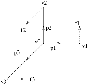
𝔣⁡(e1)=𝔭⁡(e2),𝔣⁡(e2)=𝔭⁡(e3)​𝔣​(e3)=𝔭⁡(e1).\mathfrak{f}(e_{1})=\mathfrak{p}(e_{2}),\quad\mathfrak{f}(e_{2})=\mathfrak{p}(e_{3})\mathfrak{f}(e_{3})=\mathfrak{p}(e_{1}).
Refer to caption
Figure 7. A Topological vertex with standard framing

In this section, we shall prove

Theorem 5.2 (invariance of the topological vertex).

Theorem 4.8 holds for any topological vertex with standard framing.

We fix a topological vertex with standard framing Γ\Gamma once and for all in this section; we let Y^rel=(Y^,D^)\hat{Y}^{\mathrm{rel}}=(\hat{Y},\hat{D}) be its associated FTCY threefold. As before, we continue to denote TT the group (ℂ∗)2(\mathbb{C}^{*})^{2}. We abbreviate ℳχ,d→,μ→∙​(Y^rel,L^){\cal M}_{\chi,\vec{d},{\vec{\mu}}}^{\bullet}(\hat{Y}^{\mathrm{rel}},\hat{L}) to ℳ∙​(Y^){\cal M}^{\bullet}(\hat{Y}).

Our first step to prove the invariance of

(5.1) Fχ,d→,μ→∙Γ​(u1,u2)=1|Aut⁡(μ→)|​∫[ℳ∙​(Y^)T]vireT​(𝒯1,m)eT​(𝒯2,m)∈ℚ⁡(u1/u2)F^{\bullet\Gamma}_{\chi,\vec{d},{\vec{\mu}}}(u_{1},u_{2})=\frac{1}{|\Aut({\vec{\mu}})|}\int_{[{\cal M}^{\bullet}(\hat{Y})^{T}]^{\mathrm{vir}}}\frac{e^{T}({\cal T}^{1,m})}{e^{T}({\cal T}^{2,m})}\in\mathbb{Q}(u_{1}/u_{2})

is to construct a new pair of a nonsingular projective toric threefold WW with a relative divisor D⊂WD\subset W and a subdivisor L⊂DL\subset D so that the similarly defined moduli ℳχ,d→,μ→∙​(Wrel,L){\cal M}_{\chi,\vec{d},{\vec{\mu}}}^{\bullet}(W^{\mathrm{rel}},L) (abbreviated to ℳ∙​(W){\cal M}^{\bullet}(W)) of relative stable morphisms with boundary constraint LL admits a morphism

Φ:ℳ∙​(Y^)(=ℳχ,d→,μ→∙​(Y^rel,L^))⟶ℳ∙​(W)(=ℳχ,d→,μ→∙​(Wrel,L))\Phi:{\cal M}^{\bullet}(\hat{Y})\ \bigl(={\cal M}_{\chi,\vec{d},{\vec{\mu}}}^{\bullet}(\hat{Y}^{\mathrm{rel}},\hat{L})\bigr)\longrightarrow{\cal M}^{\bullet}(W)\ \ \bigl(={\cal M}_{\chi,\vec{d},{\vec{\mu}}}^{\bullet}(W^{\mathrm{rel}},L)\bigr)

so that the induced map on the TT-fixed loci

ΦT:ℳ∙​(Y^)T⟶ℳ∙​(W)T\Phi^{T}:{\cal M}^{\bullet}(\hat{Y})^{T}\longrightarrow{\cal M}^{\bullet}(W)^{T}

has the property that it is an open and closed embedding and the obstruction theories of ℳ∙​(W){\cal M}^{\bullet}(W) along its fixed loci is identical to that of ℳ∙​(Y^){\cal M}^{\bullet}(\hat{Y}) via ΦT\Phi^{T}. Because the equality of two obstruction theories, we have the identity:

(5.2) ∫[ℳ∙​(Y^)T]vireT​(𝒯1,m)eT​(𝒯2,m)=∫[ℳ∙​(W)ΦT]vireT​(𝒯1,m)eT​(𝒯2,m),\int_{[{\cal M}^{\bullet}(\hat{Y})^{T}]^{\mathrm{vir}}}\frac{e^{T}({\cal T}^{1,m})}{e^{T}({\cal T}^{2,m})}=\int_{[{\cal M}^{\bullet}(W)^{T}_{\Phi}]^{\mathrm{vir}}}\frac{e^{T}({\cal T}^{1,m})}{e^{T}({\cal T}^{2,m})},

where ℳ∙​(W)ΦT{\cal M}^{\bullet}(W)^{T}_{\Phi} is the image of the fixed loci of ℳ∙​(Y^){\cal M}^{\bullet}(\hat{Y}). (Here by abuse of notation, we denote by 𝒯i,m{\cal T}^{i,m} the moving parts of the obstruction complex [𝒯1→𝒯2][{\cal T}^{1}\to{\cal T}^{2}] of ℳ∙​(Y^){\cal M}^{\bullet}(\hat{Y}) as well as ℳ∙​(W){\cal M}^{\bullet}(W) along their fixed loci.)

To prove the invariance of the right hand side, we shall devise a local contribution of deg⁡[ℳ∙​(W)]vir\deg[{\cal M}^{\bullet}(W)]^{\mathrm{vir}} along ℳ∙​(Y^){\cal M}^{\bullet}(\hat{Y}); this local contribution is a sum of the desired term (5.1) with some other terms; we will show that this some other terms vanish completely. This will settle the invariance of the topological vertex Γ\Gamma.

5.1. The Relative Calabi-Yau Manifold WrelW^{\mathrm{rel}} and the Morphism Φ\Phi

We begin with constructing the toric variety WrelW^{\mathrm{rel}} as promised. Looking at the graph Γ\Gamma that we chose, the obvious choice of WW is the toric blowup of ℙ1×ℙ1×ℙ1{\mathbb{P}^{1}}\times{\mathbb{P}^{1}}\times{\mathbb{P}^{1}} along three disjoint lines

(5.3) ℓ1=∞×ℙ1×0,ℓ2=0×∞×ℙ1​ℓ3=ℙ1×0×∞.\ell_{1}=\infty\times{\mathbb{P}^{1}}\times 0,\qquad\ell_{2}=0\times\infty\times{\mathbb{P}^{1}}\ell_{3}={\mathbb{P}^{1}}\times 0\times\infty.

The moment polytope of WW, which is the image of the moment map

Υ:W⟶ℝ3\Upsilon:W\longrightarrow\mathbb{R}^{3}

of the U​(1)3U(1)^{3}-action on WW, is shown in Figure 8. It is diffeomorphic to the quotient W/U​(1)3W/U(1)^{3}. Here we follow the convention that (z1,z2,z3)(z_{1},z_{2},z_{3}) is the point ([z1,1],[z2,1],[z3,1])([z_{1},1],[z_{2},1],[z_{3},1]) in (ℙ1)3({\mathbb{P}^{1}})^{3}. We let D⊂WD\subset W be the exceptional divisor and let Di⊂DD_{i}\subset D be its connected component lying over ℓi\ell_{i}. Each DiD_{i} is isomorphic to ℙ1×ℙ1{\mathbb{P}^{1}}\times{\mathbb{P}^{1}}. We then let C1,C2C_{1},C_{2} and C3C_{3} be the proper transforms of

ℙ1×0×0,0×ℙ1×00×0×ℙ1,{\mathbb{P}^{1}}\times 0\times 0,\qquad 0\times{\mathbb{P}^{1}}\times 00\times 0\times{\mathbb{P}^{1}},

and let Li⊂DiL_{i}\subset D_{i}, i=1,2i=1,2 and 33, be the preimage of

(∞,0,0)∈ℓ1,(0,∞,0)∈ℓ2​(0,0,∞)∈ℓ3.(\infty,0,0)\in\ell_{1},\qquad(0,\infty,0)\in\ell_{2}(0,0,\infty)\in\ell_{3}.

Clearly, restricting to CiC_{i} the log-canonical sheaf

(5.4) ∧3ΩW(logD)|Ci≅𝒪Ci.\wedge^{3}\Omega_{W}(\log D)|_{C_{i}}\cong{\cal O}_{C_{i}}.

Hence to the curves CiC_{i} the relative pair Wrel=(W,D)W^{\mathrm{rel}}=(W,D) is practically a relative Calabi-Yau threefold.

Refer to caption
Figure 8. Moment Polytope of WW.

All faces of this polytope represent the (ℂ∗)3(\mathbb{C}^{*})^{3} invariant divisors of WW. The point p0{p}_{0} is the image of the point (0,0,0)∈W(0,0,0)\in W. The line p0​pi¯\overline{p_{0}p_{i}} is the image of the curve Ci≅ℙ1C_{i}\cong{\mathbb{P}^{1}}, and the thickened line pi​qi¯\overline{p_{i}q_{i}} is the image of the curve Li≅ℙ1L_{i}\cong{\mathbb{P}^{1}}. The rectangle face containing the edge pi​qi¯\overline{p_{i}q_{i}} is the image of the relative divisor Di≅ℙ1×ℙ1D_{i}\cong{\mathbb{P}^{1}}\times{\mathbb{P}^{1}}.

For later discussion, we agree that under the isomorphisms Di≅ℙ1×ℙ1D_{i}\cong{\mathbb{P}^{1}}\times{\mathbb{P}^{1}} and ℓi≅ℙ1\ell_{i}\cong{\mathbb{P}^{1}}, the tautological projection Di→ℓiD_{i}\to\ell_{i} is the first projection. Under this convention, the line Li⊂DiL_{i}\subset D_{i} is the line 0×ℙ10\times{\mathbb{P}^{1}} and the intersection pi=Ci∩Dip_{i}=C_{i}\cap D_{i} is the point (0,0)(0,0).

As to the torus action, we pick the obvious one on (ℙ1)3({\mathbb{P}^{1}})^{3} via

(5.5) (z1,z2,z3)(t1,t2,t3)=(t1​z1,t2​z2,t3​z3),(t1,t2,t3)∈(ℂ∗)3.(z_{1},z_{2},z_{3})^{({t}_{1},{t}_{2},{t}_{3})}=(t_{1}z_{1},t_{2}z_{2},t_{3}z_{3}),\qquad({t}_{1},{t}_{2},{t}_{3})\in(\mathbb{C}^{*})^{3}.

It lifts to a (ℂ∗)3(\mathbb{C}^{*})^{3}-action on WW that leaves DiD_{i} and LiL_{i} invariant. We let T⊂(ℂ∗)3T\subset(\mathbb{C}^{*})^{3} be the subgroup defined by t1​t2​t3=1t_{1}t_{2}t_{3}=1; it is isomorphic to (ℂ∗)2(\mathbb{C}^{*})^{2} and is the subgroup that leaves (5.4) invariant. In the following, we shall view Wrel=(W,D)W^{\mathrm{rel}}=(W,D) as a relative Calabi-Yau TT-manifold to the curves CiC_{i}.

Next we will define the moduli space ℳχ,d→,μ→∙​(Wrel,L){\cal M}_{\chi,\vec{d},{\vec{\mu}}}^{\bullet}(W^{\mathrm{rel}},L). Clearly, each CiC_{i} induces a homology class [Ci]∈H2​(W,ℤ)[C_{i}]\in H_{2}(W;\mathbb{Z}). For

μ→=(μ1,μ2,μ3)∈𝒫+3,{\vec{\mu}}=({{\mu}^{1},{\mu}^{2},{\mu}^{3}})\in{\cal P}_{+}^{3},

we let d→\vec{d} be the homology class

d→=|μ1|​[C1]+|μ2|​[C2]+|μ3|[C3]∈H2​(W,ℤ).\vec{d}=|\mu^{1}|[C_{1}]+|\mu^{2}|[C_{2}]+|\mu^{3}|[C_{3}]\in H_{2}(W;\mathbb{Z}).

The pair (d→,μ→)(\vec{d},{\vec{\mu}}) is an effective class of Γ\Gamma:

d→(e¯i)=|μi|,μ→(vi)=μi,i=1,2,3.\vec{d}({\bar{e}}_{i})=|\mu^{i}|,\ \ {\vec{\mu}}(v_{i})=\mu^{i},\ \ i=1,2,3.

We then let

ℳχ,d→,μ→∙​(Wrel,L),abbreviate to​ℳ∙​(W),{\cal M}_{\chi,\vec{d},{\vec{\mu}}}^{\bullet}(W^{\mathrm{rel}},L),\quad\text{abbreviate to}\ {\cal M}^{\bullet}(W),

be the moduli of relative stable morphisms

u:(X,R1,R2,R3)⟶Wrel=(W,D1,D2,D3)u:(X;R_{1},R_{2},R_{3})\longrightarrow W^{\mathrm{rel}}=(W,D_{1},D_{2},D_{3})

having fundamental classes d→\vec{d}, having ramification patterns μi\mu^{i} along DiD_{i}, and satisfying u⁡(Ri)⊂Liu(R_{i})\subset L_{i}, modulo the equivalence relation introduced in [25]. It is a proper, separated DM-stack; it has a perfect obstruction theory [24, 25], and thus admits a virtual cycle.

It follows from our construction that the scheme YY, which is the the closure of the three one-dimensional orbits in Y^\hat{Y}, can be identified with the union C1∪C2∪C3C_{1}\cup C_{2}\cup C_{3} in WW; the formal scheme Y^\hat{Y} is then the formal completion of WW along YY. Further, the relative divisor D^\hat{D} of Y^\hat{Y} (resp. teh subdivisor L^⊂D^\hat{L}\subset\hat{D}) is the preimage of the relative divisor D⊂WD\subset W (resp. the subdivisor L⊂DL\subset D); the induced morphism

(5.6) ϕ:(Y^,D^,L^)⟶(W,D,L)\phi:(\hat{Y},\hat{D},\hat{L})\longrightarrow(W,D,L)

is TT-equivariant; and the two effective classes (d→,μ→)(\vec{d},{\vec{\mu}}) are consistent under the map ϕ\phi. Therefore, it induces a TT-equivariant morphism of the moduli spaces

(5.7) Φ:ℳ∙​(Y^)⟶ℳ∙​(W),\Phi:{\cal M}^{\bullet}(\hat{Y})\longrightarrow{\cal M}^{\bullet}(W),

which induces a morphism

ΦT:ℳ∙​(Y^)T⟶ℳ∙​(W)T\Phi^{T}:{\cal M}^{\bullet}(\hat{Y})^{T}\longrightarrow{\cal M}^{\bullet}(W)^{T}

between their respective fixed loci.

Lemma 5.3.

The morphism ΦT\Phi^{T} is an open and closed embedding; the obstruction theories of ℳ∙​(Y^){\cal M}^{\bullet}(\hat{Y}) and ℳ∙​(W){\cal M}^{\bullet}(W) are identical under Φ\Phi along the fixed loci ℳ∙​(Y^)T{\cal M}^{\bullet}(\hat{Y})^{T} and its image in ℳ∙​(W){\cal M}^{\bullet}(W).

Proof.

This follows immediately from that C1C_{1}, C2C_{2} and C3C_{3} are the closures of three one-dimensional orbit, that Y=C1∪C2∪C3Y=C_{1}\cup C_{2}\cup C_{3} and that Y^\hat{Y} is the formal completion of WW along YY. ∎

Later, we shall work with the moduli of relative stable morphisms ℳχ,d→,μ→∙​(Yrel,L){\cal M}_{\chi,\vec{d},{\vec{\mu}}}^{\bullet}(Y^{\mathrm{rel}},L), similarly defined as that of ℳ∙​(W){\cal M}^{\bullet}(W). Again, for notational simplicity, we shall abbreviate it to ℳ∙​(Y){\cal M}^{\bullet}(Y).

5.2. Invariant Relative Stable Morphisms

Let a1,a2,a3∈ℤa_{1},a_{2},a_{3}\in\mathbb{Z} with a1+a2+a3=0a_{1}+a_{2}+a_{3}=0 be three relatively prime integers; η=(a1,a2,a3)\eta=(a_{1},a_{2},a_{3}) defines a subgroup

Tη={(ta1,ta2,ta3)∣t∈U⁡(1)}⊂T.T_{\eta}=\{(t^{a_{1}},t^{a_{2}},t^{a_{3}})\mid t\in U(1)\}\subset T.

Our next task is to characterize those stable relative morphisms that are invariant under Tη⊂TT_{\eta}\subset T and are small deformations of elements in ℳ∙​(Y){\cal M}^{\bullet}(Y).

To investigate relative stable morphisms to WW, we need the expanded relative pair (W⁡[𝐦],D⁡[𝐦])(W[\mathbf{m}],D[\mathbf{m}]), 𝐦=(m1,m2,m3)\mathbf{m}=(m_{1},m_{2},m_{3}) (see Figure 9). Let Δ\Delta be the projective bundle ℙ⁡(𝒪ℙ1×ℙ1⊕𝒪ℙ1×ℙ1​(0,1))\mathbb{P}\bigl({\cal O}_{{\mathbb{P}^{1}}\times{\mathbb{P}^{1}}}\oplus{\cal O}_{{\mathbb{P}^{1}}\times{\mathbb{P}^{1}}}(0,1)\bigr) with two sections

D+=ℙ⁡(𝒪ℙ1×ℙ1⊕0)​D−=ℙ⁡(0⊕𝒪ℙ1×ℙ1​(0,1));D_{+}=\mathbb{P}\bigl({\cal O}_{{\mathbb{P}^{1}}\times{\mathbb{P}^{1}}}\oplus 0\bigr)D_{-}=\mathbb{P}\bigl(0\oplus{\cal O}_{{\mathbb{P}^{1}}\times{\mathbb{P}^{1}}}(0,1)\bigr);

we form an mim_{i}-chain of Δ\Delta by gluing mim_{i} copies of Δ\Delta via identifying the D−D_{-} of one Δ\Delta to the D+D_{+} of the next Δ\Delta using the canonical isomorphism pr:D±→ℙ1×ℙ1\text{pr}\!:\!D_{\pm}\to{\mathbb{P}^{1}}\times{\mathbb{P}^{1}}; we then attach this chain to DiD_{i} by identifying the D+D_{+} of the first Δ\Delta in the chain with DiD_{i} and declaring the D−D_{-} of the last Δ\Delta be D​[𝐦]iD[\mathbf{m}]_{i}. The scheme W⁡[𝐦]W[\mathbf{m}] is the result after attaching such three chains, of length m1m_{1}, m2m_{2} and m3m_{3} respectively, to D1D_{1}, D2D_{2} and D3D_{3} in WW. The union

D⁡[𝐦]=D​[𝐦]1∪D​[𝐦]2∪D​[𝐦]3D[\mathbf{m}]=D[\mathbf{m}]_{1}\cup D[\mathbf{m}]_{2}\cup D[\mathbf{m}]_{3}

is the new relative divisor of W⁡[𝐦]W[\mathbf{m}]. Note that our construction is consistent with that the normal bundle of DiD_{i} in WW has degree −1-1 along LiL_{i}.

Refer to caption
Figure 9.

This is a sketch of the scheme W⁡[𝐦]W[\mathbf{m}] for 𝐦=(0,2,0)\mathbf{m}=(0,2,0). The main part is the moment polytope of WW (see Figure 8). The added two solids to the right are the two Δ\Delta’s attached to D2D_{2}, resulting the scheme W⁡[𝐦]W[\mathbf{m}] with 𝐦=(0,2,0)\mathbf{m}=(0,2,0). The shaded faces are the relative divisor D⁡[𝐦]D[\mathbf{m}] of W⁡[𝐦]W[\mathbf{m}]. The straight diagonal line contained in the bottom face indicates the image of ϕk,c\phi_{k,c} in case η=(1,−1,0)\eta=(1,-1,0); the curved line indicates the image of ϕk,c\phi_{k,c} in the other case.

For future convenience, we denote by Δ⁡[mi]\Delta[m_{i}] the chain of Δ\Delta’s that is attached to DiD_{i}; we denote by L​[𝐦]i⊂D​[𝐦]iL[\mathbf{m}]_{i}\subset D[\mathbf{m}]_{i} the same line as Li⊂DiL_{i}\subset D_{i}. The new scheme W⁡[𝐦]W[\mathbf{m}] contains WW as its main irreducible component; it also admits a stable contraction W⁡[𝐦]→WW[\mathbf{m}]\to W. Also, (ℂ∗)3(\mathbb{C}^{*})^{3} acts on (W⁡[𝐦],D⁡[𝐦])(W[\mathbf{m}],D[\mathbf{m}]) since the (ℂ∗)3(\mathbb{C}^{*})^{3}-action on NDi/WN_{D_{i}/W} induces a (ℂ∗)3(\mathbb{C}^{*})^{3}-action on each Δ\Delta attached to DiD_{i}. Therefore (ℂ∗)3(\mathbb{C}^{*})^{3} and TT act on ℳ∙​(W){\cal M}^{\bullet}(W). Unless otherwise mentioned, the maps W→W⁡[𝐦]W\to W[\mathbf{m}] and W⁡[𝐦]→WW[\mathbf{m}]\to W are these inclusion and projection; these maps are (ℂ∗)3(\mathbb{C}^{*})^{3}-equivariant.

The pair (W,D)(W,D) contains (Y,p)(Y,p), p=p1+p2+p3p=p_{1}+p_{2}+p_{3}, as its subpair. Accordingly, the pair (W⁡[𝐦],D⁡[𝐦])(W[\mathbf{m}],D[\mathbf{m}]) contains a subpair (Y⁡[𝐦],p⁡[𝐦])(Y[\mathbf{m}],p[\mathbf{m}]) whose main part Y⁡[𝐦]Y[\mathbf{m}] is the preimage of YY under the contraction W⁡[𝐦]→WW[\mathbf{m}]\to W. The relative divisor p⁡[𝐦]p[\mathbf{m}] is the intersection Y⁡[𝐦]∩D⁡[𝐦]Y[\mathbf{m}]\cap D[\mathbf{m}]. It is the embedding Y⁡[𝐦]⊂W⁡[𝐦]Y[\mathbf{m}]\subset W[\mathbf{m}] that induces the embedding ℳ∙​(Y)⊂ℳ∙​(W){\cal M}^{\bullet}(Y)\subset{\cal M}^{\bullet}(W).

Now let u0u_{0} be a relative stable morphism in ℳ∙​(Y){\cal M}^{\bullet}(Y), considered as an element in ℳ∙​(W){\cal M}^{\bullet}(W); let usu_{s} be a small deformation of u0u_{0} in ℳ∙​(W)Tη{\cal M}^{\bullet}(W)^{T_{\eta}} that is not entirely contained in ℳ∙​(Y){\cal M}^{\bullet}(Y). Each usu_{s} is a morphism from its domain XsX_{s} to W⁡[𝐦]W[\mathbf{m}] for some triple 𝐦\mathbf{m} possibly depending on ss. We let u~s:Xs→W\tilde{u}_{s}\!:\!X_{s}\to W be the composite of usu_{s} with the contraction W⁡[𝐦]→WW[\mathbf{m}]\to W. Then u~s\tilde{u}_{s} form a flat family of morphisms; it specializes to u~0\tilde{u}_{0} as ss specializes to 00. Hence as sets, u~s​(Xs)\tilde{u}_{s}(X_{s}) specializes to u~0​(X0)\tilde{u}_{0}(X_{0}) as ss specializes to 00. Because u~s​(Xs)\tilde{u}_{s}(X_{s}) are union of algebraic curves in WW and u~0​(X0)\tilde{u}_{0}(X_{0}) is contained in C1∪C2∪C3C_{1}\cup C_{2}\cup C_{3}, for general ss the intersection u~s​(Xs)∩D\tilde{u}_{s}(X_{s})\cap D is discrete. Hence every irreducible component Z⊂u~s−1​(Di)Z\subset\tilde{u}_{s}^{-1}(D_{i}) must be mapped to a fiber of Δ⁡[mi]/Di\Delta[m_{i}]/D_{i}.

Now suppose there is such a connected component ZZ with us​(Z)u_{s}(Z) lies in the fiber of Δ⁡[mi]\Delta[m_{i}] over q∈Diq\in D_{i}, then by the pre-deformable requirement on relative stable morphisms forces the same qq in D​[𝐦]iD[\mathbf{m}]_{i} to lie in us​(Xs)u_{s}(X_{s}). Because of the requirement us​(Z)∩D​[𝐦]i⊂L​[𝐦]iu_{s}(Z)\cap D[\mathbf{m}]_{i}\subset L[\mathbf{m}]_{i} we impose on the ℳ∙​(W){\cal M}^{\bullet}(W), we have

(5.8) u~s​(Xs)∩Di⊂Li.\tilde{u}_{s}(X_{s})\cap D_{i}\subset L_{i}.

Our primary interest is to those uu that are Tη{T_{\eta}}-invariant and are small deformations of elements in ℳ∙​(Y){\cal M}^{\bullet}(Y). This leads to the following definition.

Definition 5.4.

We let Ξ⁡(η)\Xi(\eta) be the union of all connected components of

{[u,X]∈ℳ∙(W)Tη∣u~(X)∩Dis finite}\{[u,X]\in{\cal M}^{\bullet}(W)^{T_{\eta}}\mid\tilde{u}(X)\cap D\ \text{is finite}\}

that intersect ℳ∙​(Y){\cal M}^{\bullet}(Y) but are not entirely contained in it.

Following the discussion before Definition 5.4, all uu in Ξ⁡(η)\Xi(\eta) satisfies (5.8). In case ai+1≠0a_{i+1}\neq 0 (we agree a4=a1a_{4}=a_{1}), the only Tη{T_{\eta}}-fixed points of LiL_{i} are pip_{i} and qiq_{i}; hence all uu in Ξ⁡(η)\Xi(\eta) satisfies a strengthened version to (5.8):

(5.9) u~s​(X)∩Di⊂pi,when ​ai+1≠0.\tilde{u}_{s}(X)\cap D_{i}\subset p_{i},\qquad\text{when \ }a_{i+1}\neq 0.

Here qiq_{i} is ruled out because each connected component of Ξ⁡(η)\Xi(\eta) intersects ℳ∙​(Y){\cal M}^{\bullet}(Y).

We now characterize elements in Ξ⁡(η)\Xi(\eta). We comment that we shall reserve a1a_{1}, a2a_{2} and a3a_{3} for the three components of η\eta; we always assume the three aia_{i}’s are relatively prime and that a1+a2+a3=0a_{1}+a_{2}+a_{3}=0. In this and the next two Subsections, we shall workout the case a1>0a_{1}>0 and a2,a3<0a_{2},a_{3}<0; the case η=(1,−1,0)\eta=(1,-1,0) will be considered in Subsection 5.5. Now let [u,X]∈Ξ⁡(η)[u,X]\in\Xi(\eta) and let V⊂u~​(X)V\subset\tilde{u}(X) be any irreducible component. Since uu is Tη{T_{\eta}}-invariant, VV is Tη{T_{\eta}}-invariant. Hence VV must be the lift of the set

V¯={(c1​ta1,c2​t2a2,c3​t3a3)∣t∈ℂ∪{∞}}⊂(ℙ1)3\bar{V}=\{(c_{1}t^{a_{1}},c_{2}t_{2}^{a_{2}},c_{3}t_{3}^{a_{3}})\mid t\in\mathbb{C}\cup\{\infty\}\ \}\subset({\mathbb{P}^{1}})^{3}

for some (c1,c2,c3)(c_{1},c_{2},c_{3}). Thus we see that the following cases are impossible:

  1. (1)

    all cic_{i} are non-zero: should this hold, then V¯∩ℓ2=(0,∞,∞)\bar{V}\cap\ell_{2}=(0,\infty,\infty), which violates (5.8);

  2. (2)

    c1=0c_{1}=0 but the other two are non-zero: should this hold, then either V∩D=V∩D1=q1V\cap D=V\cap D_{1}=q_{1}, or V∩D=V∩D2=p2′V\cap D=V\cap D_{2}=p_{2}^{\prime} (see Figure 9 for the location of p2′p_{2}^{\prime}), so (5.9) is violated;

  3. (3)

    c2=0c_{2}=0 but the others are non-zero: should this hold, then V∩D1=q1V\cap D_{1}=q_{1} since a1>|a3|a_{1}>|a_{3}|, which violates (5.9).

This leaves us with the only two possibilities: when only one of cic_{i} is non-zero or c3=0c_{3}=0 but the other two are non-zero. In the first case we have V=CiV=C_{i} for some ii; in the later case VV is the image of the map

(5.10) ϕk,c:ℙ1⟶W,k∈ℤ+,c∈ℂ∗\phi_{k,c}:{\mathbb{P}^{1}}\longrightarrow W,\qquad k\in\mathbb{Z}^{+},\ c\in\mathbb{C}^{*}

that is the lift of ℙ1→(ℙ1)×3{\mathbb{P}^{1}}\to({\mathbb{P}^{1}})^{\times 3} defined by ξ↦(ξk​a1,c−k​a2​ξk​a2,0)\xi\mapsto(\xi^{ka_{1}},c^{-ka_{2}}\xi^{ka_{2}},0). Clearly, ϕk,c\phi_{k,c} is TηT_{\eta}-invariant. It is easy to see that these are the only Tη{T_{\eta}}-equivariant maps Z→WZ\to W from irreducible ZZ whose images are not entirely lie in C1∪C2∪C3C_{1}\cup C_{2}\cup C_{3} and the divisor DD. This proves

Lemma 5.5.

Suppose a1>0a_{1}>0 and a2a_{2}, a3<0a_{3}<0. Then any (u,X)∈Ξ⁡(η)(u,X)\in\Xi(\eta) not entirely contained in YY has at least one irreducible component Z⊂XZ\subset X and a pair (k,c)(k,c) so that u|Z≅ϕk,cu|_{Z}\cong\phi_{k,c}.

Here by u|Z≅ϕk,cu|_{Z}\cong\phi_{k,c} we mean that there is an isomorphism Z≅ℙ1Z\cong{\mathbb{P}^{1}} so that under this isomorphism u|Z≡ϕk,cu|_{Z}\equiv\phi_{k,c}.

When cc specialize to 00, the map ϕk,c\phi_{k,c} specializes to

ϕk,0:ℙ1⊔ℙ1⟶W\phi_{k,0}:{\mathbb{P}^{1}}\sqcup{\mathbb{P}^{1}}\longrightarrow W

defined as follows. We endow the first copy (of ℙ1⊔ℙ1{\mathbb{P}^{1}}\sqcup{\mathbb{P}^{1}}) with the coordinate ξ1\xi_{1} and the second copy with ξ2\xi_{2}; we then form the nodal curve ℙ1⊔ℙ1{\mathbb{P}^{1}}\sqcup{\mathbb{P}^{1}} by identifying 00 of the first ℙ1{\mathbb{P}^{1}} with 00 of the second ℙ1{\mathbb{P}^{1}}; we define ϕk,0\phi_{k,0} to be the lift of the maps

ξ1↦(ξ1k​a1,0,0)​ξ2↦(0,ξ2−k​a2,0).\xi_{1}\mapsto(\xi_{1}^{ka_{1}},0,0)\xi_{2}\mapsto(0,\xi_{2}^{-ka_{2}},0).

Since ξ1=0\xi_{1}=0 and ξ2=0\xi_{2}=0 are both mapped to the origin in (ℙ1)×3({\mathbb{P}^{1}})^{\times 3}, they glue together to form a morphism ϕk,0:ℙ1⊔ℙ1→W\phi_{k,0}\!:\!{\mathbb{P}^{1}}\sqcup{\mathbb{P}^{1}}\to W.

This leads to the following definition.

Definition 5.6.

A deformable part of a (u,X)∈Ξ⁡(η)(u,X)\in\Xi(\eta) consists of a curve Z⊂XZ\subset X and an isomorphism u|Z≅ϕk,cu|_{Z}\cong\phi_{k,c} for some (k,c)(k,c).

Suppose (u,X)(u,X) has at least two deformable parts, say (Z1,ϕk1,c1)(Z_{1},\phi_{k_{1},c_{1}}) and (Z2,ϕk1,c2)(Z_{2},\phi_{k_{1},c_{2}}), then the explicit expression of ϕk,c\phi_{k,c} ensures that Z1Z_{1} and Z2Z_{2} share no common irreducible components. Should Z1∩Z2≠∅Z_{1}\cap Z_{2}\neq\emptyset, their intersection would be a nodal point of XX that could only be mapped to either D1D_{1} or D2D_{2} of WW under uu. (Note that it could not be mapped to p0p_{0} since then both c1c_{1} and c2=0c_{2}=0, and that node would be in more than two irreducible components of XX.) However, the case that the node is mapped to D1D_{1} or D2D_{2} can also be ruled out because it violates the pre-deformable requirement of relative stable morphisms [24]. Hence Z1Z_{1} and Z2Z_{2} are disjoint. This way, we can talk about the maximal collection of deformable parts of (u,X)(u,X); let it be

(Z1,ϕk1,c1),⋯,(Zl,ϕkl,cl).(Z_{1},\phi_{k_{1},c_{1}}),\cdots,(Z_{l},\phi_{k_{l},c_{l}}).

For convenience, we order it so that kik_{i} is increasing.

Definition 5.7.

We define the deformation type of (u,X)∈Ξ⁡(η)(u,X)\in\Xi(\eta) be

(ki)l=(k1≤k2≤⋯≤kl)(k_{i})_{l}=(k_{1}\leq k_{2}\leq\cdots\leq k_{l})

It defines a function on Ξ⁡(η)\Xi(\eta), called the deformation type function.

Let (u,X)(u,X) be an element in Ξ⁡(η)\Xi(\eta) of type (ki)l(k_{i})_{l}. Intuitively, we should be able to deform uu within Ξ⁡(η)\Xi(\eta) by varying u|Ziu|_{Z_{i}} using ϕk,t\phi_{k,t} to generate an 𝔸l\mathbb{A}^{l}-family in Ξ⁡(η)\Xi(\eta). It is our next goal to make this precise.

To proceed, we need to show how to put ϕk,t\phi_{k,t} into a family. We first blow up ℙ1×𝔸1{\mathbb{P}^{1}}\times{\mathbb{A}}^{\!1} at (0,0)(0,0) to form a family of curves 𝔜\mathfrak{Y} over 𝔸1{\mathbb{A}}^{\!1}. The complement of the exceptional divisor 𝔜−E=ℙ1×𝔸1−(0,0)\mathfrak{Y}-E={\mathbb{P}^{1}}\times{\mathbb{A}}^{\!1}-(0,0) comes with an induced coordinate (ξ,t)(\xi,t). We define

Φk|𝔜−E:𝔜−E⟶W;(ξ,t)↦(ξk​a1,t−k​a2​ξk​a2,0).\Phi_{k}|_{\mathfrak{Y}-E}:\mathfrak{Y}-E\longrightarrow W;\quad(\xi,t)\mapsto(\xi^{ka_{1}},t^{-ka_{2}}\xi^{ka_{2}},0).

We claim that Φk|𝔜−E\Phi_{k}|_{\mathfrak{Y}-E} extends to a Φk:𝔜→W\Phi_{k}\!:\!\mathfrak{Y}\to W. Indeed, if we pick a local coordinate chart near EE, which is (ξ,v)(\xi,v) with t=ξ​vt=\xi v, then

Φk|𝔜−E:(ξ,v)↦(ξk​a1,(ξ​v)−k​a2​ξk​a2,0)=(ξ,v)↦(ξk​a1,v−k​a2,0),\Phi_{k}|_{\mathfrak{Y}-E}:(\xi,v)\mapsto(\xi^{ka_{1}},(\xi v)^{-ka_{2}}\xi^{ka_{2}},0)=(\xi,v)\mapsto(\xi^{ka_{1}},v^{-ka_{2}},0),

which extends to a regular

Φk:𝔜⟶W.\Phi_{k}:\mathfrak{Y}\longrightarrow W.

Note that for c∈𝔸1c\in{\mathbb{A}}^{\!1}, the fiber of (Φk,𝔜)(\Phi_{k},\mathfrak{Y}) over cc is exactly the ϕk,c\phi_{k,c} we defined earlier. Henceforth, we will call (Φk,𝔜)(\Phi_{k},\mathfrak{Y}) the standard model of the family ϕk,t\phi_{k,t}; we will use 𝔜c\mathfrak{Y}_{c} to denote the fiber of 𝔜\mathfrak{Y} over c∈𝔸1c\in{\mathbb{A}}^{\!1}.

To deform uu using the family Φk\Phi_{k}, we need to glue 𝔜\mathfrak{Y} onto the domain XX. We let 𝔇1\mathfrak{D}_{1} be the proper transform of 0×𝔸1⊂ℙ1×𝔸10\times{\mathbb{A}}^{\!1}\subset{\mathbb{P}^{1}}\times{\mathbb{A}}^{\!1} and let 𝔇2=∞×𝔸1\mathfrak{D}_{2}=\infty\times{\mathbb{A}}^{\!1} in 𝒴{\cal Y}. Both 𝔇1\mathfrak{D}_{1} and 𝔇2\mathfrak{D}_{2} are canonically isomorphic to 𝔸1{\mathbb{A}}^{\!1} via the second projection. For Z⊂XZ\subset X, we fix an isomorphism Z≅𝔜cZ\cong\mathfrak{Y}_{c} so that u|Z≅ϕk,cu|_{Z}\cong\phi_{k,c}; we specify v1v_{1}, v2∈Zv_{2}\in Z so that u⁡(vi)∈Diu(v_{i})\in D_{i}; we let X0X_{0} be the closure of X−ZX-Z in XX.

We now glue 𝔜\mathfrak{Y} onto X0×𝔸1X_{0}\times{\mathbb{A}}^{\!1}. In case both v1v_{1} and v2v_{2} are nodes of XX, we glue 𝔜\mathfrak{Y} onto X0×𝔸1X_{0}\times{\mathbb{A}}^{\!1} by identifying 𝔇1\mathfrak{D}_{1} with v1×𝔸1v_{1}\times{\mathbb{A}}^{\!1} and 𝔇2\mathfrak{D}_{2} with v2×𝔸1v_{2}\times{\mathbb{A}}^{\!1}, using the their standard isomorphisms with 𝔸1{\mathbb{A}}^{\!1}; in case v1v_{1} is a marked point of XX and v2v_{2} is a node, we glue 𝔜\mathfrak{Y} onto X0×𝔸1X_{0}\times{\mathbb{A}}^{\!1} by identifying 𝔇2\mathfrak{D}_{2} with v2×𝔸1v_{2}\times{\mathbb{A}}^{\!1} and declaring 𝔇1\mathfrak{D}_{1} to be the new marked points, replacing v1v_{1}; in case v1v_{1} is a node and v2v_{2} is a marked points, we repeat the same procedure with the role of v1v_{1} and v2v_{2} and of 𝔇1\mathfrak{D}_{1} and 𝔇2\mathfrak{D}_{2} exchanged; finally in case both v1v_{1} and v2v_{2} are marked points, we simply replace Z×𝔸1Z\times{\mathbb{A}}^{\!1} in X×𝔸1X\times{\mathbb{A}}^{\!1} by 𝔜\mathfrak{Y} while declaring that 𝔇1\mathfrak{D}_{1} and 𝔇2\mathfrak{D}_{2} are the two marked points replacing v1v_{1} and v2v_{2}. We let 𝒳→𝔸1{\cal X}\to{\mathbb{A}}^{\!1} be the resulting family.

The morphisms

X0×𝔸1−⁣⟶prX0−⁣⟶u|X0W[𝐦]Φk:𝔜−⁣⟶WX_{0}\times{\mathbb{A}}^{\!1}\,\smash{\mathop{-\!\!\!\longrightarrow}\limits^{\rm{pr}}}\,X_{0}\,\smash{\mathop{-\!\!\!\longrightarrow}\limits^{u|_{X_{0}}}}\,W[\mathbf{m}]\Phi_{k}:\mathfrak{Y}\,\smash{\mathop{-\!\!\!\longrightarrow}\limits}\,W

glue together to form a morphism

𝒰:𝒳⟶W⁡[𝐦].{\cal U}:{\cal X}\longrightarrow W[\mathbf{m}].

The pair (𝒰,𝒳)({\cal U},{\cal X}) is the family in Ξ⁡(η)\Xi(\eta) that keeps u|X0u|_{X_{0}} fixed.

More generally, we can deform uu inside Ξ⁡(η)\Xi(\eta) by identifying and altering its restriction to the deformable parts of XX simultaneously. This way, any u∈Ξ⁡(η)u\in\Xi(\eta) of type (ki)l(k_{i})_{l} generates an 𝔸l\mathbb{A}^{l} family of elements in Ξ⁡(η)\Xi(\eta).

5.3. Global Structure of the Loci of Invariant Relative Morphisms

In this subsection, we shall prove that any connected component of Ξ⁡(η)\Xi(\eta) is an 𝔸l\mathbb{A}^{l}-bundle.

We begin with a technical Lemma

Lemma 5.8.

Let v∈Xnodev\in X_{\text{node}} be a node in u−1​(D)u^{-1}(D). Then vv remains a node when uu deforms infinitesimally in Ξ⁡(η)\Xi(\eta).

The key to the proof relies on the fact that the restrictions of the automorphisms induced by Tη{T_{\eta}} on one irreducible component of XX that contains vv are infinite while on the other irreducible component are finite.

Recall that there is an natural inclusion h:T→Aut⁡(W⁡[𝐦])h:T\to\Aut(W[\mathbf{m}]) induced by the TT-actions on WW and on NDi/WN_{D_{i}/W}. There is a unique homomorphism h′:T→Aut⁡(W⁡[𝐦]/W)h^{\prime}:T\to\Aut(W[\mathbf{m}]/W) such that33 3 The automorphisms ζ∈Aut⁡(W⁡[𝐦])\zeta\in\Aut(W[\mathbf{m}]) that preserve the fibers of the map W⁡[𝐦]→WW[\mathbf{m}]\to W are called relative automorphisms of W⁡[𝐦]/WW[\mathbf{m}]/W; the group of all such automorphisms is denoted by Aut⁡(W⁡[𝐦]/W)\Aut(W[\mathbf{m}]/W). If 𝐦=(m1,m2,m3)\mathbf{m}=(m_{1},m_{2},m_{3}) then Aut⁡(W⁡[𝐦]/W)≅(ℂ∗)m1+m2+m3\Aut(W[\mathbf{m}]/W)\cong(\mathbb{C}^{*})^{m_{1}+m_{2}+m_{3}}. h′​(t)∘h⁡(t)∈Aut⁡(W⁡[𝐦])h^{\prime}(t)\circ h(t)\in\Aut(W[\mathbf{m}]) acts trivially on pi​[mi]p_{i}[m_{i}], the fiber of Δ⁡[mi]\Delta[m_{i}] over pi∈Dip_{i}\in D_{i}, for all t∈Tt\in T. Since uu is TηT_{\eta}-invariant and the image u⁡(u−1​(Δ⁡[mi]))u\bigl(u^{-1}(\Delta[m_{i}])\bigr) is entiredly contained in pi​[mi]p_{i}[m_{i}], there are group homomorphisms h1:Tη→Aut⁡(X)h_{1}\!:\!{T_{\eta}}\to\Aut(X) and h2:Tη→Aut⁡(W⁡[𝐦]/W)h_{2}\!:\!{T_{\eta}}\to\Aut(W[\mathbf{m}]/W) so that for all σ∈Tη\sigma\in{T_{\eta}},

(5.11) (i) h′(σ)∘h(σ)∘u=h2(σ)∘u∘h1(σ)(ii) h2(σ) acts on pi[mi] trivially.\textup{(i) }h^{\prime}(\sigma)\circ h(\sigma)\circ u=h_{2}(\sigma)\circ u\circ h_{1}(\sigma)\textup{(ii) }h_{2}(\sigma)\textup{ acts on }p_{i}[m_{i}]\textup{ trivially}.

Now let v∈u−1​(Di)v\in u^{-1}(D_{i}) be a node of XX that is mapped to DiD_{i} under uu; let V−V_{-} be the irreducible component of XX that contains vv that is mapped to WW and let V+V_{+} be the other irreducible component of XX that contains vv. Then u⁡(V+)u(V_{+}) must be contained in Δ⁡[mi]\Delta[m_{i}]. Since h1​(id)=idh_{1}(\id)=\id and that Tη{T_{\eta}} is connected, h1​(σ)​(V±)⊂V±h_{1}(\sigma)(V_{\pm})\subset V_{\pm}. Hence h1​(σ)h_{1}(\sigma) are automorphisms of V±V_{\pm} that fixed vv. We let

Tη|V±=def{h1​(σ)∣σ∈Tη}⊂Aut⁡(V±,v);{T_{\eta}}|_{V_{\pm}}\stackrel{{\scriptstyle\mathrm{def}}}{{=}}\{h_{1}(\sigma)\mid\sigma\in{T_{\eta}}\}\subset\Aut(V_{\pm},v);

it is a group which is a homomorphism image of Tη≅U⁡(1)T_{\eta}\cong U(1), so it is either U⁡(1)U(1) or trivial.

Lemma 5.9.

The group Tη|V−{T_{\eta}}|_{V_{-}} is infinite while the group Tη|V+{T_{\eta}}|_{V_{+}} is finite. So Tη|V−≅U⁡(1){T_{\eta}}|_{V_{-}}\cong U(1) and Tη|V+{T_{\eta}}|_{V_{+}} is trivial.

Proof.

The group Tη|V−{T_{\eta}}|_{V_{-}} is infinite is obvious. Since u⁡(v)=piu(v)=p_{i} and u⁡(V−)⊂Wu(V_{-})\subset W, u⁡(V−)u(V_{-}) is Tη{T_{\eta}} invariant but not Tη{T_{\eta}} fixed. Since the induced action on u⁡(V−)u(V_{-}) is infinite, Tη|V−{T_{\eta}}|_{V_{-}} must be infinite because uu is Tη{T_{\eta}}-invariant.

Note that u⁡(V+)u(V_{+}) must be contained in pi​[mi]p_{i}[m_{i}] for some ii. By (5.11),

u|V+=u∘h1​(σ)|V+:V+⟶pi​[mi]∀σ∈Tη.u|_{V_{+}}=u\circ h_{1}(\sigma)|_{V_{+}}:V_{+}\longrightarrow p_{i}[m_{i}]\quad\forall\sigma\in{T_{\eta}}\,.

By stability of the relative morphism uu, Tη|V+T_{\eta}|_{V_{+}} is finite. ∎

We now prove Lemma 5.8.

Proof of Lemma 5.8.

Suppose vv can be smoothed at least of first order within Ξ⁡(η)\Xi(\eta). Since Ξ⁡(η)\Xi(\eta) is fixed by Tη{T_{\eta}}, Tη|V−{T_{\eta}}|_{V_{-}} is infinite forces Tη|V+{T_{\eta}}|_{V_{+}} to be infinite as well. This violates the assumption that Tη|V+{T_{\eta}}|_{V_{+}} is finite. This proves the Lemma. ∎

As we argued before, each u∈Ξ⁡(η)u\in\Xi(\eta) contains a deformable part that is the union of some ϕki,ci\phi_{k_{i},c_{i}}. Our next task is to show the deformable part of uu remain the same within a connected component of Ξ⁡(η)\Xi(\eta).

We make it more precise now. We let (u,X)(u,X) be any element in Ξ⁡(η)\Xi(\eta); let Y1,⋯,Yl⊂XY_{1},\cdots,Y_{l}\subset X be all its deformable parts so that u|Yi≅ϕki,ciu|_{Y_{i}}\cong\phi_{k_{i},c_{i}}; we let vi,1v_{i,1} and vi,2∈Yiv_{i,2}\in Y_{i} be the marked points so that u⁡(vi,j)=pju(v_{i,j})=p_{j}. Then according to the discussion in the previous Subsection, by varying u|Yiu|_{Y_{i}} using Φki\Phi_{k_{i}} we get a copy 𝔸1{\mathbb{A}}^{\!1} in Ξ⁡(η)\Xi(\eta); together they provide a copy 𝔸l\mathbb{A}^{l} in Ξ⁡(η)\Xi(\eta). This is one of the fiber of the fiber bundle structure on Ξ⁡(η)\Xi(\eta) we are about to construct.

To extend this 𝔸l⊂Ξ⁡(η)\mathbb{A}^{l}\subset\Xi(\eta) to nearby elements of [u][u], we need to extend all YiY_{i} in XX to a flat family of subcurves.

Lemma 5.10.

The deformation type function on Ξ⁡(η)\Xi(\eta) is locally constant.

Proof.

We pick an analytic disk 0∈S0\in S and an analytic map ψ:S→ℳ∙​(W)defTη\psi\!:\!S\to{\cal M}^{\bullet}(W)^{T_{\eta}}_{\mathrm{def}} so that ψ⁡(0)=[u]\psi(0)=[u]. The morphism ψ\psi pulls back the tautological family on Ξ⁡(η)\Xi(\eta) to a family 𝒰:𝒳→𝒵{\cal U}\!:\!{\cal X}\to{\cal Z} over SS. The central fiber 𝒳0{\cal X}_{0} is XX and thus contains YiY_{i}. We let 𝒩⊂𝒳{\cal N}\subset{\cal X} be the subscheme of the nodes of all fibers of 𝒳/S{\cal X}/S. Since vi,jv_{i,j} is either a marked point or a node of XX, vi,j∈𝒩∪ℛv_{i,j}\in{\cal N}\cup{\cal R}. Let 𝒫i,j{\cal P}_{i,j} be the connected component of 𝒩∪ℛ{\cal N}\cup{\cal R} that contains vi,jv_{i,j}. We claim that 𝒫i,j{\cal P}_{i,j} is a section of 𝒩∪ℛ→S{\cal N}\cup{\cal R}\to S. First, 𝒫i,j{\cal P}_{i,j} is flat over SS at vi,jv_{i,j}. This is true in case vi,jv_{i,j} is a marked point since ℛ{\cal R} is flat over SS by definition; in case vi,jv_{i,j} is a node it is true because of Lemma 5.8. Therefore, 𝒫i,j{\cal P}_{i,j} dominates over SS. Then because 𝒩∪ℛ{\cal N}\cup{\cal R} is proper and unramified over SS, dominating over SS guarantees that 𝒫i,j{\cal P}_{i,j} is finite and étale over SS. But then since SS is a disk, 𝒫i,j{\cal P}_{i,j} must be isomorphic to SS via the projection.

We now pick the desired family of curves 𝒴i{\cal Y}_{i}. In case 𝒫i,j{\cal P}_{i,j} is one of the section of the marked points of 𝒳/S{\cal X}/S, we do nothing; otherwise, we resolve the singularity of the fibers of 𝒳{\cal X} along 𝒫i,j{\cal P}_{i,j}. As a result, we obtain a flat family of subcurves 𝒴i⊂𝒳{\cal Y}_{i}\subset{\cal X} that contains YiY_{i} as its central fiber. We let 𝒰i:𝒴i→𝒲{\cal U}_{i}\!:\!{\cal Y}_{i}\to{\cal W} be the restriction of 𝒰{\cal U} to 𝒴i{\cal Y}_{i}. Because 𝒰i​(Yi)⊂W⊂W⁡[𝐦]{\cal U}_{i}(Y_{i})\subset W\subset W[\mathbf{m}], 𝒰i​(𝒴i)⊂W×S⊂𝒲{\cal U}_{i}({\cal Y}_{i})\subset W\times S\subset{\cal W} as well.

Since 𝒰:𝒳→𝒲{\cal U}\!:\!{\cal X}\to{\cal W} is a family of Tη{T_{\eta}}-equivariant relative stable maps, 𝒰i:𝒴i→W{\cal U}_{i}\!:\!{\cal Y}_{i}\to W is also a family of Tη{T_{\eta}}-equivariant stable morphisms. Then because 𝒰i|Yi{\cal U}_{i}|_{Y_{i}} is isomorphic to ϕki,ci\phi_{k_{i},c_{i}}, each member of 𝒰i{\cal U}_{i} must be an ϕki,c\phi_{k_{i},c} for some c∈ℂc\in\mathbb{C}. This proves that the deformation type of 𝒰|𝒳s{\cal U}|_{{\cal X}_{s}} contains that of 𝒰|𝒳0{\cal U}|_{{\cal X}_{0}} as a subset. Because this holds true with 00 and ss exchanged, it shows that the deformation type function stay constant over SS.

Finally, because any two elements in the same connected component of Ξ⁡(η)\Xi(\eta) can be connected by a chain of analytic disks, the deformation type function does take same values on such component. This proves the lemma. ∎

We are now ready to exhibit a fiber bundle structure of any connected component of Ξ⁡(η)\Xi(\eta). Let 𝒬⊂Ξ⁡(η){\cal Q}\subset\Xi(\eta) be any connected component. According to the previous subsection, all elements in 𝒬{\cal Q} are of the same deformation types, say (ki)l(k_{i})_{l}. In case 𝒬{\cal Q} is not entirely contained in ℳ∙​(Y){\cal M}^{\bullet}(Y), then necessarily l>0l>0. To get the fiber structure, we need to take a finite cover of 𝒬{\cal Q}, which we now construct.

Definition 5.11.

We define the groupoid 𝒬¯\bar{\cal Q} over 𝒬{\cal Q} as follows. For any scheme SS over 𝒬{\cal Q}, we let 𝒬¯​(S)\bar{\cal Q}(S) be the collection of data {(𝒰,𝒳,𝒲),ρi,𝒵i,πi∣i=1⋯,l}\{({\cal U},{\cal X},{\cal W}),\rho_{i},{\cal Z}_{i},\pi_{i}\mid i=1\cdots,l\} of which

  1. (1)

    𝒰:𝒳→𝒲{\cal U}\!:\!{\cal X}\to{\cal W} is an object 44 4 Here we consider 𝒬{\cal Q} as a groupoid and 𝒬⁡(S){\cal Q}(S) is the collection of objects over SS. in 𝒬⁡(S){\cal Q}(S)

  2. (2)

    ρi\rho_{i} are morphisms from SS to 𝔸i1{\mathbb{A}}^{\!1}_{i}, 𝔸i1≅𝔸1{\mathbb{A}}^{\!1}_{i}\cong{\mathbb{A}}^{\!1};

  3. (3)

    𝒵i{\cal Z}_{i} are flat families of subcurves in 𝒳{\cal X} over SS with all marked points discarded;

  4. (4)

    πi:𝒵i→ρi∗​𝔜ki\pi_{i}\!:\!{\cal Z}_{i}\to\rho_{i}^{*}\mathfrak{Y}_{k_{i}} an isomorphism over SS;

together they satisfy

𝒰|𝒵i≡ρi∗​Φki∘πi:𝒵i⟶W.{\cal U}|_{{\cal Z}_{i}}\equiv\rho_{i}^{*}\Phi_{k_{i}}\circ\pi_{i}:{\cal Z}_{i}\longrightarrow W.

Further, an arrow from {(𝒰,𝒳,𝒲),ρi,𝒵i,πi}\{({\cal U},{\cal X},{\cal W}),\rho_{i},{\cal Z}_{i},\pi_{i}\} to {(𝒰′,𝒳′.𝒲′),ρi′,𝒵i′,πi′}\{({\cal U}^{\prime},{\cal X}^{\prime}.{\cal W}^{\prime}),\rho_{i}^{\prime},{\cal Z}_{i}^{\prime},\pi_{i}^{\prime}\} consists of an isomorphism h1:𝒳→𝒳′h_{1}\!:\!{\cal X}\to{\cal X}^{\prime} and an isomorphism h2:𝒲→𝒲′h_{2}\!:\!{\cal W}\to{\cal W}^{\prime} relative to WW so that under these isomorphisms 𝒵i=𝒵i′{\cal Z}_{i}={\cal Z}_{i}^{\prime}, ρi=ρi′\rho_{i}=\rho_{i}^{\prime}, πi=πi′\pi_{i}=\pi_{i}^{\prime} (for all ii) and 𝒰=𝒰′{\cal U}={\cal U}^{\prime}.

Here we use 𝔸i1{\mathbb{A}}^{\!1}_{i} to denote the target of ρi\rho_{i}, which is 𝔸1{\mathbb{A}}^{\!1}. We are doing this to distinguish them for different ii.

For a fixed type (ki)l(k_{i})_{l}, we let G(ki)G_{(k_{i})} be the group {σ∈Sl∣kσ⁡(i)=ki}\{\sigma\in S_{l}\mid k_{\sigma(i)}=k_{i}\}.

Proposition 5.12.

The groupoid 𝒬¯\bar{\cal Q} is a DM-stack acted on by G(ki)G_{(k_{i})} ; it is finite and étale over 𝒬{\cal Q}, and 𝒬¯/G(ki)=𝒬\bar{\cal Q}/G_{(k_{i})}={\cal Q}. The morphisms ρi\rho_{i} in each object in 𝒬¯\bar{\cal Q} glue to a morphism ρ¯i:𝒬¯→𝔸i1\bar{\rho}_{i}\!:\!\bar{\cal Q}\to{\mathbb{A}}^{\!1}_{i}. Let 𝒬¯0=(ρ¯1,⋯,ρ¯l)−1​(0)\bar{\cal Q}_{0}=(\bar{\rho}_{1},\cdots,\bar{\rho}_{l})^{-1}(0). Then there is a canonical projection π:𝒬¯→𝒬¯0\pi\!:\!\bar{\cal Q}\to\bar{\cal Q}_{0} making it an 𝔸l\mathbb{A}^{l}-bundle over 𝒬¯0\bar{\cal Q}_{0}. Finally, the morphism

(π,(ρ¯1,⋯,ρ¯l)):𝒬¯⟶𝒬¯0×𝔸l(\pi,(\bar{\rho}_{1},\cdots,\bar{\rho}_{l})):\bar{\cal Q}\longrightarrow\bar{\cal Q}_{0}\times\mathbb{A}^{l}

is an isomorphism of DM-stacks.

Proof.

The proof is straightforward, following the previous discussion, and will be omitted. ∎

5.4. The Obstruction Sheaves

In this subsection, we will investigate the obstruction sheaf to deforming a [u][u] in Ξ⁡(η)\Xi(\eta) for the case a2a_{2}, a3<0a_{3}<0; we will follow the convention introduced in Subsection 5.3.

We let S→𝒬¯S\to\bar{\cal Q} be an TT-equivariant étale neighborhood, we let

𝒰:𝒳⟶𝒲,ℛ⊂𝒳,𝒟⊂𝒲𝒵i⊂𝒳{\cal U}:{\cal X}\longrightarrow{\cal W},\quad{\cal R}\subset{\cal X},\quad{\cal D}\subset{\cal W}{\cal Z}_{i}\subset{\cal X}

be the tautological family of SS of Ξ⁡(η)\Xi(\eta). Here 𝒲{\cal W} is an SS-family of W⁡[𝐦]W[\mathbf{m}] of possibly varying 𝐦\mathbf{m}, 𝒟{\cal D} is the relative divisor of 𝒲{\cal W}, ℛ⊂𝒳{\cal R}\subset{\cal X} is the sections marked points and 𝒵i⊂𝒳{\cal Z}_{i}\subset{\cal X} is the i-th deformable parts of 𝒰{\cal U}.

Let 𝒯2{\cal T}^{2} be the obstruction sheaf over S{S} of the obstruction theory of Ξ⁡(η)\Xi(\eta). According to [25], its Tη{T_{\eta}}-invariant part, indicated by the subscript (⋅)Tη(\cdot)_{T_{\eta}}, fits into the long exact sequences

(5.12) ⟶ℰ​𝑥𝑡𝒳/S1(Ω𝒳/S(ℛ),𝒪𝒳)Tη⟶β𝒜Tη1⟶δ𝒯~Tη2⟶0;\longrightarrow\ext^{1}_{{\cal X}/S}(\Omega_{{\cal X}/S}({\cal R}),{\cal O}_{{\cal X}})_{T_{\eta}}\,\smash{\mathop{\longrightarrow}\limits^{\beta}}\,{\cal A}^{1}_{T_{\eta}}\,\smash{\mathop{\longrightarrow}\limits^{\delta}}\,\tilde{\cal T}^{2}_{T_{\eta}}\longrightarrow 0;
(5.13) ⟶ℬTη0⟶R1π∗(𝒰∗Ω𝒲†/S(log𝒟)∨)Tη⟶α𝒜Tη1⟶ℬTη1⟶0\longrightarrow{\cal B}^{0}_{T_{\eta}}\,\smash{\mathop{\longrightarrow}\limits}\,R^{1}\pi_{\ast}\bigl({\cal U}^{*}\Omega_{{\cal W}^{\dagger}/{S}}(\log{\cal D})^{\vee}\bigr)_{T_{\eta}}\,\smash{\mathop{\longrightarrow}\limits^{\alpha}}\,{\cal A}^{1}_{T_{\eta}}\,\smash{\mathop{\longrightarrow}\limits}\,{\cal B}^{1}_{T_{\eta}}\longrightarrow 0

and

(5.14) ⟶𝒯~Tη1⟶ℋTη⟶𝒯Tη2⟶𝒯~Tη2⟶0.\longrightarrow\tilde{\cal T}^{1}_{T_{\eta}}\longrightarrow{\cal H}_{T_{\eta}}\,\smash{\mathop{\longrightarrow}\limits}\,{\cal T}^{2}_{T_{\eta}}\longrightarrow\tilde{\cal T}^{2}_{T_{\eta}}\longrightarrow 0.

Within these sequences, ℬi=⊕j=13ℬij{\cal B}^{i}=\oplus_{j=1}^{3}{\cal B}^{i}_{j}; each summand ℬji{\cal B}^{i}_{j} is a sheaf that associates to the smoothing of the nodes of the fibers of 𝒳{\cal X} that are mapped under 𝒰{\cal U} to DD (⊂W\subset W) and the singular loci of Δ⁡[mi]\Delta[m_{i}]; the 𝒲†{\cal W}^{\dagger} is the scheme 𝒲{\cal W} with the log structure defined in [25] and Ω𝒲†\Omega_{{\cal W}^{\dagger}} is the sheaf of log differentials. In our case, 𝒰∗​Ω𝒲†/S​(𝒟)=𝒰~∗​ΩW​(log⁡D){\cal U}^{*}\Omega_{{\cal W}^{\dagger}/{S}}({\cal D})=\tilde{\cal U}^{*}\Omega_{W}(\log D), where 𝒰~:𝒳→W\tilde{\cal U}\!:\!{\cal X}\to W is the obvious induced morphism.

Without taking the Tη{T_{\eta}}-invariant part, the top two exact sequences define the obstruction sheaf 𝒯~2\tilde{\cal T}^{2} to deforming [u][u] in ℳχ,d→,μ→∙​(Wrel){{\cal M}_{\chi,\vec{d},{\vec{\mu}}}^{\bullet}(W^{\mathrm{rel}})} — the moduli of relative stable morphisms to WrelW^{\mathrm{rel}} without requiring u⁡(R)⊂Lu(R)\subset L. Taking the invariant part and adding the last exact sequence defines the obstruction sheaf 𝒯Tη2{\cal T}^{2}_{T_{\eta}} of Ξ⁡(η)\Xi(\eta). The sheaf ℋ{\cal H} is the pull back of the normal line bundle to ℒ⊂𝒟{\cal L}\subset{\cal D}. For the η\eta we are interested, ℋTη=0{\cal H}_{T_{\eta}}=0; hence the last exact sequence reduces to 𝒯Tη2≡𝒯~Tη2{\cal T}^{2}_{T_{\eta}}\equiv\tilde{\cal T}^{2}_{T_{\eta}}.

In the following we shall show that the ll families 𝒵i⊂𝒳{\cal Z}_{i}\subset{\cal X} of deformable parts of (𝒰,𝒳)({\cal U},{\cal X}) each contributes to a weight zero trivial quotient sheaf of 𝒯Tη2{\cal T}^{2}_{T_{\eta}}.

We begin with the sheaf

(5.15) R1πk∗(Φk∗ΩW(logD)∨),R^{1}\pi_{k\ast}\bigl(\Phi_{k}^{*}\Omega_{W}(\log D)^{\vee}\bigr),

where Φki:𝔜→W\Phi_{k_{i}}\!:\!\mathfrak{Y}\to W is the family constructed before and πk:𝔜→𝔸1\pi_{k}\!:\!\mathfrak{Y}\to{\mathbb{A}}^{\!1} is the projection. We let D12{D}_{12} (resp. D31{D}_{31}) be the TT-invariant divisor of WW that contains C1C_{1} and C2C_{2} (resp. C1C_{1} and C3C_{3}); it is also the proper transform of the product of the first and second (resp. the first and third) copies of ℙ1{\mathbb{P}^{1}} in (ℙ1)3({\mathbb{P}^{1}})^{3}. We let π12:W→D12\pi_{12}\!:\!W\to{D}_{12}, π31:W→D31\pi_{31}\!:\!W\to{D}_{31} and π1:W→C1\pi_{1}\!:\!W\to C_{1} be the obvious projections. We claim that ΩW​(log⁡D)|D12\Omega_{W}(\log D)|_{D_{12}} has a direct summand π1∗​𝒩C1/D31∨\pi_{1}^{*}{\cal N}_{C_{1}/{D}_{31}}^{\vee}. Indeed, via the projection π31\pi_{31} we have homomorphism

π31∗​𝒩C1\D31∨|D12⟶ΩW|D12⟶ΩW​(log⁡D)|D12.\pi_{31}^{*}{\cal N}^{\vee}_{C_{1}\backslash D_{31}}|_{D_{12}}\longrightarrow\Omega_{W}|_{D_{12}}\longrightarrow\Omega_{W}(\log D)|_{D_{12}}.

Also via the projection π12\pi_{12} we have homomorphism

π12∗​ΩD12​(log⁡E12)|D12⟶ΩW​(log⁡D)|D12,E12=D12∩W.\pi_{12}^{*}\Omega_{D_{12}}(\log E_{12})|_{D_{12}}\longrightarrow\Omega_{W}(\log D)|_{D_{12}},\quad E_{12}=D_{12}\cap W.

Combined, we have

π31∗​𝒩C1\D31∨|D12⊕π12∗​ΩD12​(log⁡E12)|D12⟶ΩW​(log⁡D)|D12,\pi_{31}^{*}{\cal N}^{\vee}_{C_{1}\backslash D_{31}}|_{D_{12}}\oplus\pi_{12}^{*}\Omega_{D_{12}}(\log E_{12})|_{D_{12}}\longrightarrow\Omega_{W}(\log D)|_{D_{12}},

which can easily be shown an isomorphism. This proves that ΩW​(log⁡D)|D12\Omega_{W}(\log D)|_{D_{12}} has a direct summand π1∗​𝒩C1/D31∨\pi_{1}^{*}{\cal N}_{C_{1}/{D}_{31}}^{\vee}. Consequently, Φk∗​ΩW​(log⁡D)∨\Phi_{k}^{*}\Omega_{W}(\log D)^{\vee} has a direct summand Φk∗​(π1∗​𝒩C1/D31)\Phi_{k}^{*}(\pi_{1}^{*}{\cal N}_{C_{1}/{D}_{31}}).

Because of our choice, the weight of d​zidz_{i} is aia_{i}; the weight of T0∨​𝔜cT_{0}^{\vee}\mathfrak{Y}_{c} at 00 is 1/ki1/k_{i} and the weight of Φk∗​(π1∗​𝒩C1/D31)\Phi_{k}^{*}(\pi^{*}_{1}{\cal N}_{C_{1}/{D}_{31}}) at 0×𝔸1⊂𝔜0\times{\mathbb{A}}^{\!1}\subset\mathfrak{Y} is −a3-a_{3}. Hence, the sheaf (5.15) splits to line bundles of weights

−a3−a1+1k,−a3−a1+2k,⋯⋯,−a3−1k.-a_{3}-a_{1}+\frac{1}{k},\,-a_{3}-a_{1}+\frac{2}{k},\cdots\cdots,-a_{3}-\frac{1}{k}.

Since all aia_{i} are integers, and a3≤−1a_{3}\leq-1 and −a3−a1=a2≤−1-a_{3}-a_{1}=a_{2}\leq-1, within the above list there is exactly one that is zero. Hence

(5.16) R1πk∗(Φk∗ΩW(logD)∨)Tη≅𝒪𝔸1.R^{1}\pi_{k\ast}\bigl(\Phi_{k}^{*}\Omega_{W}(\log D)^{\vee}\bigr)_{T_{\eta}}\cong{\cal O}_{{\mathbb{A}}^{\!1}}.

We now let ρi:S→𝔸i1\rho_{i}\!:\!{S}\to{\mathbb{A}}^{\!1}_{i} be so that 𝒰|𝒵i≅ρi∗​Φki{\cal U}|_{{\cal Z}_{i}}\cong\rho_{i}^{*}\Phi_{k_{i}}. Since 𝒵i⊂𝒳{\cal Z}_{i}\subset{\cal X} is a flat family of subcurves,

R1​π∗​(𝒰∗​Ω𝒲†/S​(log⁡𝒟)∨)Tη⟶R1​π∗​(𝒰∗​Ω𝒲†/S​(log⁡𝒟)∨|𝒵i)TηR^{1}\pi_{\ast}\bigl({\cal U}^{*}\Omega_{{\cal W}^{\dagger}/{S}}(\log{\cal D})^{\vee}\bigr)_{T_{\eta}}\longrightarrow R^{1}\pi_{\ast}\bigl({\cal U}^{*}\Omega_{{\cal W}^{\dagger}/{S}}(\log{\cal D})^{\vee}|_{{\cal Z}_{i}}\bigr)_{T_{\eta}}

is surjective; but the last term is isomorphic to the pull back ρi∗\rho_{i}^{*} of (5.16); hence we obtain a quotient sheaf

(5.17) φi:R1​π∗​(𝒰∗​Ω𝒲†/S​(log⁡𝒟)∨)Tη⟶ρi∗​𝒪𝔸i1.\varphi_{i}:R^{1}\pi_{\ast}\bigl({\cal U}^{*}\Omega_{{\cal W}^{\dagger}/S}(\log{\cal D})^{\vee}\bigr)_{T_{\eta}}\longrightarrow\rho_{i}^{*}{\cal O}_{{\mathbb{A}}^{\!1}_{i}}.
Lemma 5.13.

The homomorphism φi\varphi_{i} canonically lifts to surjective

(5.18) φ^i:𝒯Tη2⟶ρi∗​𝒪𝔸i1.\hat{\varphi}_{i}:{\cal T}^{2}_{T_{\eta}}\longrightarrow\rho_{i}^{*}{\cal O}_{{\mathbb{A}}^{\!1}_{i}}.

The default proof is to follow the construction of the sheaves and the exact sequences in (5.12-5.14); once it is done, the required vanishing will follow immediately. However, to follow this strategy, we need to set up the notation as in [25] that itself requires a lot of efforts. Instead, we will utilize the decomposition of SS to give a more conceptual argument; bypassing some straightforward but tedious checking.

We first decompose 𝒰{\cal U} into four subfamilies. Since 𝒲/S{\cal W}/S is a family of expanded pairs of (W,D)(W,D), 𝒲[0]=W×S{\cal W}^{[0]}=W\times S is a closed subscheme of 𝒲{\cal W}. We then let 𝒳[0]=𝒰−1​(𝒲[0]){\cal X}^{[0]}={\cal U}^{-1}({\cal W}^{[0]}). Because of Lemma 5.8,

𝒰[0]=𝒰|𝒳[0]:𝒳[0]⟶𝒲[0]{\cal U}^{[0]}={\cal U}|_{{\cal X}^{[0]}}:{\cal X}^{[0]}\longrightarrow{\cal W}^{[0]}

is an SS-family of relative stable morphisms relative to 𝒟[0]=D×S⊂𝒲[0]{\cal D}^{[0]}=D\times S\subset{\cal W}^{[0]}. Next we consider the composite

𝒰~:𝒳⟶𝒲⟶𝒲[0]\tilde{\cal U}:{\cal X}\longrightarrow{\cal W}\longrightarrow{\cal W}^{[0]}

and the preimage 𝒰~−1​(Di)\tilde{\cal U}^{-1}(D_{i}). Because of the same reason, either this preimage is a flat family of nodes over SS or is a flat family of curves over SS. In the former case we agree 𝒳[i]=∅{\cal X}^{[i]}=\emptyset and in the later case we define

𝒳[i]=𝒰~−1​(Di×S),𝒰[i]=𝒰|𝒳[i]:𝒳[i]⟶𝒲[i],{\cal X}^{[i]}=\tilde{\cal U}^{-1}(D_{i}\times S),\quad{\cal U}^{[i]}={\cal U}|_{{\cal X}^{[i]}}:{\cal X}^{[i]}\longrightarrow{\cal W}^{[i]},

where the last term 𝒲[i]{\cal W}^{[i]} is the SS-family of Δ⁡[mi]\Delta[m_{i}]’s that were attached to 𝒲[0]{\cal W}^{[0]} along Di×SD_{i}\times S to form 𝒲{\cal W}.

Since 𝒰[0]:𝒳[0]→𝒲[0]{\cal U}^{[0]}\!:\!{\cal X}^{[0]}\to{\cal W}^{[0]} is a family of Tη{T_{\eta}}-equivariant relative stable morphisms, and since 𝒰[i]{\cal U}^{[i]} is a family of Tη{T_{\eta}}-equivariant relative stable morphisms to Δ\Delta relative to D−D_{-} and D+D_{+}, modulo an additional equivalence induced by the ℂ∗\mathbb{C}^{*} action on Δ\Delta, the obstruction sheaves 𝒯[i],2{\cal T}^{[i],2} over SS to deforming 𝒰[i]{\cal U}^{[i]} as Tη{T_{\eta}}-equivariant maps fit into similar exact sequences

(5.19) ⟶ℰ​𝑥𝑡𝒳[i]/S1(Ω𝒳[i]/S^(ℛ[i]),𝒪𝒳[i])Tη⟶β[i]𝒜Tη[i],1⟶δ[i]𝒯Tη[i],2⟶0\longrightarrow\ext^{1}_{{\cal X}^{[i]}/S}(\Omega_{{\cal X}^{[i]}/\hat{S}}({\cal R}^{[i]}),{\cal O}_{{\cal X}^{[i]}})_{T_{\eta}}\,\smash{\mathop{\longrightarrow}\limits^{\beta^{[i]}}}\,{\cal A}^{[i],1}_{T_{\eta}}\,\smash{\mathop{\longrightarrow}\limits^{\delta^{[i]}}}\,{\cal T}^{[i],2}_{T_{\eta}}\longrightarrow 0

and

(5.20) ⟶ℬTη[i],0⟶R1π∗(𝒰[i]∗Ω𝒲[i]†/S(log𝒟)∨)Tη⟶α[i]𝒜Tη[i],1⟶ℬTη[i],1⟶0.\longrightarrow{\cal B}^{[i],0}_{T_{\eta}}\,\smash{\mathop{\longrightarrow}\limits}\,R^{1}\pi_{\ast}\bigl({\cal U}^{[i]\ast}\Omega_{{\cal W}^{[i]\dagger}/S}(\log{\cal D})^{\vee}\bigr)_{T_{\eta}}\,\smash{\mathop{\longrightarrow}\limits^{\alpha^{[i]}}}\,{\cal A}^{[i],1}_{T_{\eta}}\,\smash{\mathop{\longrightarrow}\limits}\,{\cal B}^{[i],1}_{T_{\eta}}\longrightarrow 0.

Here we have already used the observation that 𝒯~Tη[i],2=𝒯Tη[i],2\tilde{\cal T}^{[i],2}_{T_{\eta}}={\cal T}^{[i],2}_{T_{\eta}}.

Now let 𝒩sp⊂𝒰−1​(Di×S){\cal N}_{\text{sp}}\subset{\cal U}^{-1}(D_{i}\times S) be any section of nodes of 𝒳{\cal X} that separates 𝒳[0]{\cal X}^{[0]} and 𝒳[i]{\cal X}^{[i]}. By Lemma 5.9, the induced Tη{T_{\eta}}-automorphisms on the connected component of 𝒳[0]{\cal X}^{[0]} adjacent to 𝒩sp{\cal N}_{\text{sp}} is infinite and on 𝒳[i]{\cal X}^{[i]} is finite. Therefore the Tη{T_{\eta}}-invariant parts

ℰ​𝑥𝑡𝒳/S1​(Ω𝒳/S​(ℛ),𝒪𝒳)Tη=⊕i=03ℰ​𝑥𝑡𝒳[i]/S1​(Ω𝒳[i]/S​(ℛ[i]),𝒪𝒳[i])Tη.\ext^{1}_{{\cal X}/S}(\Omega_{{\cal X}/S}({\cal R}),{\cal O}_{{\cal X}})_{T_{\eta}}=\mathop{\oplus}_{i=0}^{3}\ext^{1}_{{\cal X}^{[i]}/S}(\Omega_{{\cal X}^{[i]}/S}({\cal R}^{[i]}),{\cal O}_{{\cal X}^{[i]}})_{T_{\eta}}.

For the similar reason, because the tangent bundle Tpi​WT_{p_{i}}W has no weight 00 non-trivial Tη{T_{\eta}}-invariant subspaces,

(5.21) R1π∗(𝒰∗Ω𝒲†/S(log𝒟)∨)Tη=⊕i=03R1π∗(𝒰[i]∗Ω𝒲[i]†/S(log𝒟[i])∨)Tη,R^{1}\pi_{\ast}\bigl({\cal U}^{\ast}\Omega_{{\cal W}^{\dagger}/S}(\log{\cal D})^{\vee}\bigr)_{T_{\eta}}=\mathop{\oplus}_{i=0}^{3}R^{1}\pi_{\ast}\bigl({\cal U}^{[i]\ast}\Omega_{{\cal W}^{[i]\dagger}/S}(\log{\cal D}^{[i]})^{\vee}\bigr)_{T_{\eta}},

where 𝒟[i]{\cal D}^{[i]} is the relative divisor of 𝒲[i]{\cal W}^{[i]}. Further, if we follow the definition of the sheaves ℬi{\cal B}^{i} and 𝒜i{\cal A}^{i}, we can prove that

(5.22) ⊕i=03𝒜Tη[i],j=𝒜Tηj​⊕i=03ℬTη[i],j=ℬTηj;\mathop{\oplus}_{i=0}^{3}{\cal A}^{[i],j}_{T_{\eta}}={\cal A}^{j}_{T_{\eta}}\mathop{\oplus}_{i=0}^{3}{\cal B}^{[i],j}_{T_{\eta}}={\cal B}^{j}_{T_{\eta}};

that under these isomorphisms,

(5.23) ⊕i=03α[i]=α,⊕i=03β[i]=β​⊕i=03δ[i]=δ;\mathop{\oplus}_{i=0}^{3}\alpha^{[i]}=\alpha,\quad\mathop{\oplus}_{i=0}^{3}\beta^{[i]}=\beta\mathop{\oplus}_{i=0}^{3}\delta^{[i]}=\delta;

and

(5.24) ⊕i=03𝒯Tη[i],2=𝒯Tη2.\mathop{\oplus}_{i=0}^{3}{\cal T}^{[i],2}_{T_{\eta}}={\cal T}^{2}_{T_{\eta}}.

Finally, the exact sequences (5.12) and (5.13) become the direct sums of the exact sequences (5.19) and (5.20).

Now we come back to the weight zero quotient φi\varphi_{i} in (5.17). By its construction, φi\varphi_{i} is merely the canonical quotient homomorphism

(5.25) R1π∗(𝒰[0]∗Ω𝒲[0]/S(log𝒟[0])∨)Tη⟶R^{1}\pi_{\ast}\bigl({\cal U}^{[0]\ast}\Omega_{{\cal W}^{[0]}/S}(\log{\cal D}^{[0]})^{\vee}\bigr)_{T_{\eta}}\longrightarrow\qquad\qquad
⟶R1π∗(𝒰[0]∗Ω𝒲[0]/S(log𝒟[0])∨|𝒵i)Tη=ρi∗𝒪𝔸i1.\qquad\qquad\qquad\qquad\longrightarrow R^{1}\pi_{\ast}\bigl({\cal U}^{[0]\ast}\Omega_{{\cal W}^{[0]}/S}(\log{\cal D}^{[0]})^{\vee}|_{{\cal Z}_{i}}\bigr)_{T_{\eta}}=\rho^{*}_{i}{\cal O}_{{\mathbb{A}}^{\!1}_{i}}.

under the isomorphism (5.21). Because of (5.24), to lift φi\varphi_{i} to φ^i\hat{\varphi}_{i} we only need to lift (5.25) to 𝒯Tη[0],2→ρi∗​𝒪𝔸i1{\cal T}^{[0],2}_{T_{\eta}}\to\rho^{*}_{i}{\cal O}_{{\mathbb{A}}^{\!1}_{i}}.

For this, we need to look at the exact sequence (5.20) for 𝒳[0]{\cal X}^{[0]}. Since 𝒰[0]{\cal U}^{[0]} is a relative stable map to (W,D)(W,D) — namely no Δ\Delta’s has been attached to WW — the sheaf ℬ[0],j=0{\cal B}^{[0],j}=0. Therefore the sequence (5.20) reduces to α[0]=id\alpha^{[0]}=\text{id}. On the other hand, 𝒯Tη[0],2{\cal T}^{[0],2}_{T_{\eta}} is the obstruction sheaf on SS to deformations of 𝒰[0]{\cal U}^{[0]}. Since 𝒵i{\cal Z}_{i} is a family of connected components of 𝒳[0]/S{\cal X}^{[0]}/S, the exact sequence (5.19) decomposes into direct sum of individual exact sequences that contains

(5.26) ⟶ℰ​𝑥𝑡𝒵i/S1(Ω𝒵i/S^(ℛ[0]),𝒪𝒵i)Tη⟶β[𝒵^i]\longrightarrow\ext^{1}_{{\cal Z}_{i}/S}\bigl(\Omega_{{\cal Z}_{i}/\hat{S}}({\cal R}^{[0]}),{\cal O}_{{\cal Z}_{i}}\bigr)_{T_{\eta}}\,\smash{\mathop{\longrightarrow}\limits^{\beta^{[\hat{\cal Z}_{i}]}}}\,\hskip 20.44434pt\hskip 20.44434pt\hskip 20.44434pt
⟶R1π∗(𝒰[0]∗Ω𝒲†/S^(log𝒟)∨|𝒵i)Tη⟶δ[𝒵i]𝒯Tη[𝒵i],2⟶0,\qquad\qquad\qquad\longrightarrow R^{1}\pi_{\ast}\bigl({\cal U}^{[0]\ast}\Omega_{{\cal W}^{\dagger}/\hat{S}}(\log{\cal D})^{\vee}|_{{\cal Z}_{i}}\bigr)_{T_{\eta}}\,\smash{\mathop{\longrightarrow}\limits^{\delta^{[{\cal Z}_{i}]}}}\,{\cal T}^{[{\cal Z}_{i}],2}_{T_{\eta}}\longrightarrow 0,

as its factors.

For 𝒵i{\cal Z}_{i}, since it is smooth, it has expected dimension zero and has actual dimension one, the obstruction sheaf 𝒯Tη[𝒵i],2{\cal T}^{[{\cal Z}_{i}],2}_{T_{\eta}} must be a rank one locally free sheaf on SS. Then because the middle term in (5.26) is ρi∗​𝒪𝔸i1\rho_{i}^{*}{\cal O}_{{\mathbb{A}}^{\!1}_{i}}, which is a rank one locally free sheaf, the arrow δ[𝒵i]\delta^{[{\cal Z}_{i}]} must be an isomorphism while β[𝒵i]=0\beta^{[{\cal Z}_{i}]}=0. Hence φi\varphi_{i} lifts to

𝒯Tη[0],2≡⊕j𝒯Tη[𝒵j],2⟶𝒯Tη[𝒵i],2≡ρi∗​𝒪𝔸i1,{\cal T}^{[0],2}_{T_{\eta}}\equiv\mathop{\oplus}_{j}{\cal T}^{[{\cal Z}_{j}],2}_{T_{\eta}}\longrightarrow{\cal T}^{[{\cal Z}_{i}],2}_{T_{\eta}}\equiv\rho_{i}^{*}{\cal O}_{{\mathbb{A}}^{\!1}_{i}},

and lifts to φ^i:𝒯Tη2→ρi∗​𝒪𝔸i1\hat{\varphi}_{i}\!:\!{\cal T}^{2}_{T_{\eta}}\to\rho_{i}^{*}{\cal O}_{{\mathbb{A}}^{\!1}_{i}}, thanks to (5.24).

5.5. The Case for η=(1,−1,0)\eta=(1,-1,0)

We now investigate the structures of maps [u]∈Ξ⁡(η)[u]\in\Xi(\eta) in case η=(1,−1,0)\eta=(1,-1,0). Let (u,X)(u,X) be any such map, let RR be the marked points and let u~\tilde{u} be the contraction X→WX\to W. Because a3=0a_{3}=0, u~​(X)\tilde{u}(X) intersects D1D_{1} at p1p_{1}; intersects D3D_{3} at p3p_{3} while intersects D2D_{2} can be any point in L2L_{2}. Thus being Tη{T_{\eta}}-equivariant forces u~​(X)\tilde{u}(X) to be a finite union of a subset of C1C_{1}, C2C_{2}, C3C_{3} and the lifts of the sets {z1​z2=c,z3=0}⊂(ℙ1)3\{z_{1}z_{2}=c,z_{3}=0\}\subset({\mathbb{P}^{1}})^{3}.

In case all irreducible components are mapped to ∪Ci\cup\,C_{i} under u~\tilde{u}, [u]∈ℳ∙​(Y)[u]\in{\cal M}^{\bullet}(Y). For those that are not in ℳ∙​(Y){\cal M}^{\bullet}(Y), there bound to be some Y⊂XY\subset X so that u~​(Y)\tilde{u}(Y) is the lifts of {z1​z2=c,z3=0}\{z_{1}z_{2}=c,z_{3}=0\}. Such u|Yu|_{Y} are realized by the morphism ϕk,c:ℙ1→W\phi_{k,c}\!:\!{\mathbb{P}^{1}}\to W that are the lifts of

(5.27) ξ↦(ck​ξk,ξ−k,0)∈(ℙ1)3.\xi\mapsto(c^{k}\xi^{k},\xi^{-k},0)\in({\mathbb{P}^{1}})^{3}.

When cc specializes to 00, the map ϕk,c\phi_{k,c} specializes to ϕk,0:ℙ1⊔ℙ1→W\phi_{k,0}\!:\!{\mathbb{P}^{1}}\sqcup{\mathbb{P}^{1}}\to W that is the lift of ξ1↦(ξ1k,0,0)\xi_{1}\mapsto(\xi_{1}^{k},0,0) and ξ2↦(0,ξ2−k,0)\xi_{2}\mapsto(0,\xi_{2}^{-k},0). Indeed, there is a family 𝔜→𝔸1\mathfrak{Y}\to{\mathbb{A}}^{\!1} and a morphism Φk:𝔜→W\Phi_{k}\!:\!\mathfrak{Y}\to W so that its fiber over c∈𝔸1c\in{\mathbb{A}}^{\!1} is the ϕk,c\phi_{k,c} defined; also this is a complete list Tη{T_{\eta}}-equivariant deformations of ϕk,c\phi_{k,c}. Since the argument is exactly the same as in the case studied, we shall not repeat it here.

Here comes the main difference between this and the case studied earlier. In the previous case, Im⁡ϕk,c∩Di=pi\image\phi_{k,c}\cap D_{i}=p_{i} for both i=1i=1 and 22; hence we can deform each u|Y≅ϕk,cu|_{Y}\cong\phi_{k,c} to produce an 𝔸1{\mathbb{A}}^{\!1} family in Ξ⁡(η)\Xi(\eta). In the case under consideration, though Im⁡ϕk,c∩D1=p1\image\phi_{k,c}\cap D_{1}=p_{1}, if we fix an embedding 𝔸1⊂L2{\mathbb{A}}^{\!1}\subset L_{2} so that 0∈𝔸10\in{\mathbb{A}}^{\!1} is the p2∈L2p_{2}\in L_{2}, then Im⁡ϕk,c∩D2=ck∈L2\image\phi_{k,c}\cap D_{2}=c^{k}\in L_{2}. In other words, if we deform u|F≅ϕk,cu|_{F}\cong\phi_{k,c}, we need to move the connected component of X[2]X^{[2]} that is connected to YY.

This leads to the following definition.

Definition 5.14.

We say that a connected component Y⊂X[0]Y\subset X^{[0]} is subordinated to a connected component E⊂X[2]E\subset X^{[2]} if Y∩E≠∅Y\cap E\neq\emptyset; we say a connected component E⊂X[2]E\subset X^{[2]} is deformable if every connected component of X[0]X^{[0]} that is subordinate to EE is of the form ϕk,c\phi_{k,c} for some pair (k,c)(k,c). We say uu has deformation type (ki)l=(k1≤⋯≤kl)(k_{i})_{l}=(k_{1}\leq\cdots\leq k_{l}) if it has exactly ll deformable connected components ϕk1,c1,⋯,ϕkl,cl\phi_{k_{1},c_{1}},\cdots,\phi_{k_{l},c_{l}} in X[2]X^{[2]}.

The deformation types define a function on Ξ⁡(η)\Xi(\eta).

Lemma 5.15.

The deformation type function is locally constant on Ξ⁡(η)\Xi(\eta).

Proof.

The proof is parallel to the case studied, and will be omitted. ∎

As in the previous case, any [u]∈Ξ⁡(η)[u]\in\Xi(\eta) of deformation type (ki)l(k_{i})_{l} generates an 𝔸l\mathbb{A}^{l} in Ξ⁡(η)\Xi(\eta) so that its origin lies in ℳ∙​(Y){\cal M}^{\bullet}(Y). Let E1,⋯,El⊂X[2]E_{1},\cdots,E_{l}\subset X^{[2]} be the complete set of deformable parts of uu; let Yi,jY_{i,j}, j=1,⋯,nij=1,\cdots,n_{i} be the complete set of connected components in X[0]X^{[0]} that are subordinate to EiE_{i}. By definition, each u|Yi,j≅ϕki,j,ci,ju|_{Y_{i,j}}\cong\phi_{k_{i,j},c_{i,j}}. To deform uu, we shall vary the ci,jc_{i,j} in each ϕki,j,ci,j\phi_{k_{i,j},c_{i,j}} and move EiE_{i} accordingly to get a new map.

In accordance, we shall divide XX into three parts. We let X0X_{0} be the union of irreducible components of XX other than the EiE_{i}’s and Yi,jY_{i,j}’s. The variation of uu will remain unchanged over this part of the curve. The second part is the moving part EiE_{i}’s. Recall that each u|Eiu|_{E_{i}} is a morphism to Δ⁡[m2]\Delta[m_{2}]. Suppose it maps to the fiber Δ​[m2]c\Delta[m_{2}]_{c} of Δ⁡[m2]\Delta[m_{2}] over c∈L2⊂D2c\in L_{2}\subset D_{2}. To deform uu, we need to make the new map maps EiE_{i} to Δ​[m2]c′\Delta[m_{2}]_{c^{\prime}}. Since the total space of Δ⁡[m2]\Delta[m_{2}] over L2L_{2} is a trivial ℙ1​[m2]{\mathbb{P}^{1}}[m_{2}] bundle, there is a canonical way to do this. We let

φc,c′:Δ​[m2]c​−⁣⟶≅⁡Δ​[m2]c′\varphi_{c,c^{\prime}}:\Delta[m_{2}]_{c}\,\smash{\mathop{-\!\!\!\longrightarrow}\limits^{\cong}}\,\Delta[m_{2}]_{c^{\prime}}

be the isomorphism of the two fibers of Δ⁡[m2]\Delta[m_{2}] over cc and c′∈L2c^{\prime}\in L_{2} induced by the projection Δ⁡[m2]→ℙ1​[m2]\Delta[m_{2}]\to{\mathbb{P}^{1}}[m_{2}] that is induced by the product structure on Δ⁡[m2]\Delta[m_{2}] over L2L_{2}. The third parts are those Yi,jY_{i,j} that are subordinate to EiE_{i}.

We now deform the map uu using the parameter space 𝔸l\mathbb{A}^{l}. We let KiK_{i} be the least common multiple of (ki,1,⋯,ki,ni)(k_{i,1},\cdots,k_{i,n_{i}}); we let ei,j=Ki/ki,je_{i,j}=K_{i}/k_{i,j}. Since Yi,jY_{i,j} and Yi,j′Y_{i,j^{\prime}} are connected to the same connected component Ei⊂X[2]E_{i}\subset X^{[2]}, ci,jki,j=ci,j′ki,j′c_{i,j}^{k_{i,j}}=c_{i,j^{\prime}}^{k_{i,j^{\prime}}}; we let it be cic_{i}. For 𝐭=(t1,⋯,tl)∈𝔸l\mathbf{t}=(t_{1},\cdots,t_{l})\in\mathbb{A}^{l}, we define

(5.28) u𝐭|X0=u|X0,u𝐭|Ei=φci,tiKi∘u|Ei​u𝐭|Yi,j=ϕki,j,tiei,j.u^{\mathbf{t}}|_{X_{0}}=u|_{X_{0}},\quad u^{\mathbf{t}}|_{E_{i}}=\varphi_{c_{i},t_{i}^{K_{i}}}\circ u|_{E_{i}}u^{\mathbf{t}}|_{Y_{i,j}}=\phi_{k_{i,j},t_{i}^{e_{i,j}}}.

Here in case Yi,j≅ℙ1Y_{i,j}\cong{\mathbb{P}^{1}}, which is the case when ci,j≠0c_{i,j}\neq 0, by u𝐭|Yi,j=ϕki,j,0u^{\mathbf{t}}|_{Y_{i,j}}=\phi_{k_{i,j},0} we mean that we will replace Yi,jY_{i,j} by ℙ1⊔ℙ1{\mathbb{P}^{1}}\sqcup{\mathbb{P}^{1}} with necessarily gluing if required; and vice versa.

The 𝔸l\mathbb{A}^{l} family u𝐭u^{\mathbf{t}} is a family of Tη{T_{\eta}}-equivariant relative stable morphisms in Ξ⁡(η)\Xi(\eta); the map u0u^{0} associated to 0∈𝔸l0\in\mathbb{A}^{l} lies in ℳ∙​(Y){\cal M}^{\bullet}(Y); the induced morphism 𝔸l→Ξ⁡(η)\mathbb{A}^{l}\to\Xi(\eta) is an embedding up to a finite quotient.

By extending this to any connected component 𝒬{\cal Q} of Ξ⁡(η)\Xi(\eta), we obtain

Proposition 5.16.

Let 𝒬{\cal Q} be any connected component of Ξ⁡(η)\Xi(\eta) that is not entirely contained in ℳ∙​(Y){\cal M}^{\bullet}(Y). Suppose elements of 𝒬{\cal Q} has deformation type (ki)l(k_{i})_{l}. Then there is a stack 𝒬¯\bar{\cal Q}, a finite quotient morphism 𝒬¯/G(ki)→𝒬\bar{\cal Q}/G_{(k_{i})}\to{\cal Q}, a closed substack 𝒬¯0⊂𝒬¯\bar{\cal Q}_{0}\subset\bar{\cal Q}, ll projections ρi:𝒬¯→𝔸i1\rho_{i}\!:\!\bar{\cal Q}\to{\mathbb{A}}^{\!1}_{i} and a projection π:𝒬¯→𝒬¯0\pi\!:\!\bar{\cal Q}\to\bar{\cal Q}_{0} so that

(π,(ρ1,⋯,ρl)):𝒬¯​−⁣⟶≅⁡𝒬¯0×𝔸l\bigl(\pi,(\rho_{1},\cdots,\rho_{l})\bigr):\bar{\cal Q}\,\smash{\mathop{-\!\!\!\longrightarrow}\limits^{\cong}}\,\bar{\cal Q}_{0}\times\mathbb{A}^{l}

is an isomorphism. Further, given a [u]∈𝒬[u]\in{\cal Q}, the fiber 𝔸l\mathbb{A}^{l} in 𝒬¯\bar{\cal Q} that contains a lift of [u]∈𝒬[u]\in{\cal Q} is the 𝔸l\mathbb{A}^{l} family {u𝐭∣𝐭∈𝔸l}\{u^{\mathbf{t}}\mid\mathbf{t}\in\mathbb{A}^{l}\}; its intersection with the zero section 𝒬¯0\bar{\cal Q}_{0} is u0u^{0}. Finally, the intersection 𝒬∩ℳ∙​(Y){\cal Q}\cap{\cal M}^{\bullet}(Y) is the image of 𝒬¯0\bar{\cal Q}_{0}.

Proof.

Let 𝒰:𝒳→𝒲{\cal U}\!:\!{\cal X}\to{\cal W} be the tautological family over 𝒬¯\bar{\cal Q}. We choose 𝒬¯\bar{\cal Q} so that there are families of subcurves ℰ1,⋯,ℰl⊂𝒳{\cal E}_{1},\cdots,{\cal E}_{l}\subset{\cal X} so that for each z∈𝒬¯z\in\bar{\cal Q}, ℰ1∩𝒳z,⋯,ℰl∩𝒳z{\cal E}_{1}\cap{\cal X}_{z},\cdots,{\cal E}_{l}\cap{\cal X}_{z} are exactly the ll deformable parts of 𝒳z{\cal X}_{z}. Then the composite ℰi→𝒲⟶W{\cal E}_{i}\to{\cal W}\longrightarrow W factor through L2⊂WL_{2}\subset W, and the resulting morphism ℰi→L2{\cal E}_{i}\to L_{2} factor through 𝒬¯→L2\bar{\cal Q}\to L_{2}. Because each ℰi∩𝒳z{\cal E}_{i}\cap{\cal X}_{z} has a ϕk,c\phi_{k,c} connected to it, the image of 𝒬¯→L2\bar{\cal Q}\to L_{2} lies in L2−q2L_{2}-q_{2}. We then fix an isomorphism 𝔸1≅L2−q2{\mathbb{A}}^{\!1}\cong L_{2}-q_{2} with 00 corresponding to p2p_{2}. This way we obtain the desired morphism

ρi:𝒬¯⟶𝔸i1≅L2−q2.\rho_{i}:\bar{\cal Q}\longrightarrow{\mathbb{A}}^{\!1}_{i}\cong L_{2}-q_{2}.

The proof of the remainder part of the Proposition is exactly the same as the case studied; we shall not repeat it here. ∎

The last step is to investigate the obstruction sheaf over 𝒬{\cal Q}, or its lift to 𝒬¯\bar{\cal Q}.

Let ℛ⊂𝒳{\cal R}\subset{\cal X} the divisor of marked points. By passing to an étale covering of 𝒬¯\bar{\cal Q}, we can assume that ℛ→𝒬{\cal R}\to{\cal Q} is a union of sections; in other words, we can index the marked points of [u][u] in 𝒬¯\bar{\cal Q} globally. We then pick an indexing so that for i≤li\leq l the ii-th section of the marked points ℛi{\cal R}_{i} lies in ℰi{\cal E}_{i}. For i=1,…,ni=1,\ldots,n, where nn is the number of marked points, we let 𝒰i:𝒬¯→ℒ2{\cal U}_{i}\!:\!\bar{\cal Q}\to{\cal L}_{2} be

𝒰i=def𝒰|ℛi:ℛi≅𝒬¯⟶ℒ2⊂𝒲.{\cal U}_{i}\stackrel{{\scriptstyle\mathrm{def}}}{{=}}{\cal U}|_{{\cal R}_{i}}:{\cal R}_{i}\cong\bar{\cal Q}\longrightarrow{\cal L}_{2}\subset{\cal W}.

Since ℒ2⊂𝒟2{\cal L}_{2}\subset{\cal D}_{2} is isomorphic to L2×𝒬¯⊂D2×𝒬¯L_{2}\times\bar{\cal Q}\subset D_{2}\times\bar{\cal Q} under the contraction 𝒲→W×𝒬¯{\cal W}\to W\times\bar{\cal Q} and since ℛi{\cal R}_{i} lies in ℰi{\cal E}_{i}, for i≤li\leq l the morphism 𝒰i{\cal U}_{i} is exactly the ρi\rho_{i} under the isomorphism 𝔸i1≅L2−q2{\mathbb{A}}^{\!1}_{i}\cong L_{2}-q_{2}, and 𝒰i∗​𝒩ℒ/𝒟{\cal U}_{i}^{*}{\cal N}_{{\cal L}/{\cal D}} is canonically isomorphic to ρi∗​NL2/D2\rho_{i}^{*}N_{L_{2}/D_{2}}. Because D2D_{2} is fixed by Tη{T_{\eta}}, NL2/D2N_{L_{2}/D_{2}} is fixed as well, and hence ρi∗​NL2/D2\rho_{i}^{*}N_{L_{2}/D_{2}} is a trivial line bundle on 𝒬¯\bar{\cal Q} with trivial Tη{T_{\eta}}-linearization.

Because ℋ=⊕i=1n𝒰i∗𝒩ℒ/𝒟{\cal H}=\oplus_{i=1}^{n}{\cal U}_{i}^{*}{\cal N}_{{\cal L}/{\cal D}} (see Section 5.4), ⊕i=1lρ∗iNL2/D2\oplus_{i=1}^{l}\rho^{*}_{i}N_{L_{2}/D_{2}} becomes a direct summand of ℋ{\cal H}. Because it has weight zero, it induces a canonical homomorphism

⊕i=1lρ∗iNL2/D2⟶𝒯2Tη,\oplus_{i=1}^{l}\rho^{*}_{i}N_{L_{2}/D_{2}}\longrightarrow{\cal T}^{2}_{T_{\eta}},

a weight zero subsheaf of 𝒯Tη2{\cal T}^{2}_{T_{\eta}}.

Lemma 5.17.

The homomorphism ⊕i=1lρi∗NL2/D2→𝒯2Tη\oplus_{i=1}^{l}\rho_{i}^{*}N_{L_{2}/D_{2}}\to{\cal T}^{2}_{T_{\eta}} in (5.14) is injective; thus 𝒯Tη2{\cal T}^{2}_{T_{\eta}} contains ⊕i=1lρi∗NL2/D2\oplus_{i=1}^{l}\rho_{i}^{*}N_{L_{2}/D_{2}} as its subsheaf. Indeed, this subsheaf is canonically a direct summand of 𝒯Tη2{\cal T}^{2}_{T_{\eta}}.

Proof.

First the first ll marked points lie in the connected components of X[2]X^{[2]} that are connected to the domain of at least one ϕk,c\phi_{k,c} in WW. Because all deformations of ϕk,c\phi_{k,c} as Tη{T_{\eta}}-invariant maps are ϕk,c′\phi_{k,c^{\prime}}, and they intersect D2D_{2} in L2L_{2} only; hence for these ii even if we do not impose the condition 𝒰⁡(ℛi)⊂ℒ2{\cal U}({\cal R}_{i})\subset{\cal L}_{2} the condition will be satisfied automatically. In short, the arrow 𝒯~Tη1→ℋTη\tilde{\cal T}^{1}_{T_{\eta}}\to{\cal H}_{T_{\eta}} has image lies in the summand ⊕i=l+1n𝒰∗i𝒩ℒ/𝒟\oplus_{i=l+1}^{n}{\cal U}^{*}_{i}{\cal N}_{{\cal L}/{\cal D}}. This proves that the homomorphism ⊕i=1lρi∗NL2/D2→𝒯2Tη\oplus_{i=1}^{l}\rho_{i}^{*}N_{L_{2}/D_{2}}\to{\cal T}^{2}_{T_{\eta}} is injective.

We now show that this subsheaf is canonically a summand of the obstruction sheaf. The ordinary moduli of stable relative morphisms ℳχ,d→,μ→∙​(Wrel){\cal M}_{\chi,\vec{d},{\vec{\mu}}}^{\bullet}(W^{\mathrm{rel}}) requires that the marked points be sent to the relative divisor. The moduli space ℳ∙​(W)=ℳχ,d→,μ→∙​(Wrel,L){\cal M}^{\bullet}(W)={\cal M}_{\chi,\vec{d},{\vec{\mu}}}^{\bullet}(W^{\mathrm{rel}},L) we worked on imposes one more restriction: the marked points be sent to L⊂DL\subset D. The obstruction sheaves of the two moduli spaces are related by the exact sequence (5.14) because of the exact sequences

0⟶NLi/Di⟶NLi/W⟶NDi/W|Li⟶0.0\longrightarrow N_{L_{i}/D_{i}}\longrightarrow N_{L_{i}/W}\longrightarrow N_{D_{i}/W}|_{L_{i}}\longrightarrow 0.

In our case, LiL_{i} is a ℙ1{\mathbb{P}^{1}} and the above exact sequence splits TT-equivariantly. Hence the sheaf 𝒯Tη2{\cal T}^{2}_{T_{\eta}} splits off a factor that is the kernel of 𝒯~Tη1→ℋTη\tilde{\cal T}^{1}_{T_{\eta}}\to{\cal H}_{T_{\eta}}. Therefore ⊕li=1ρi∗NL2/D2\oplus^{l}_{i=1}\rho_{i}^{*}N_{L_{2}/D_{2}}, which is a summand of ℋTη{\cal H}_{T_{\eta}} and a subsheaf of 𝒯Tη2{\cal T}^{2}_{T_{\eta}}, becomes a summand 𝒯Tη2{\cal T}^{2}_{T_{\eta}}. ∎

5.6. A Criterion for Constancy

We first remark that due to the nature of the discussion in the remainder of this section, we shall use analytic topology of instead of Zariski topology. In particular, unless otherwise specified, all open sets will be analytic open sets. Accordingly, we shall view DM-stack as orbifold with analytic topology.

Before we proceed to the details of the proof, a quick review of the construction of the virtual cycles of the moduli stack is in order. Let T=(ℂ∗)2T=(\mathbb{C}^{*})^{2} as before and let MM be a proper Deligne-Mumford stack acted on by TT and endowed with a TT-equivariant perfect obstruction theory. As shown in [3, 4, 28], the virtual cycle [M]vir[M]^{\mathrm{vir}} is constructed by

  1. a.

    identifying the perfect obstruction theory of MM;

  2. b.

    picking a vector bundle55 5 It was shown in [25] the existence of a global vector bundle EE can be replaced by that MM is dominated by a quasi-projective scheme. (locally free sheaf) EE on MM so that it surjects onto the obstruction sheaf of MM and

  3. c.

    constructing an associated cone C⊂EC\subset E of pure dimension rank⁡E\rank E.

The virtual cycle [M]vir[M]^{\mathrm{vir}} is the image of the cycle [C]∈H∗​(E,E−M)[C]\in H_{*}(E,E-M) under the Thom isomorphism

φE:H∗​(E,E−M)⟶H∗−2​r​(M),r=rank⁡E.\varphi_{E}:H_{*}(E,E-M)\longrightarrow H_{*-2r}(M),\quad r=\rank E.

Here as usual, we denote by EE the total space of EE and denote by M⊂EM\subset E its zero section that is isomorphic to MM. Also, all (co)homologies are taken with ℚ\mathbb{Q} coefficient.

Following [15], we can make the above construction TT-equivariant. We choose EE be a TT-equivariant vector bundle. Then the cone CC alluded before is a TT-invariant subcone of E{E}. Because C⊂EC\subset{E} is TT-equivariant, the composite

T×C⟶pr2C⟶ET\times C\,\smash{\mathop{\longrightarrow}\limits^{\text{pr}_{2}}}\,C\longrightarrow{E}

defines a TT-equivariant [C]T∈H∗T​(E,E−M)[C]^{T}\in H^{T}_{\ast}({E},{E}-M); its image under the TT-equivariant Thom isomorphism φE\varphi_{E} is the TT-equivariant virtual moduli cycle

φE​([C]T)=[M]vir,T∈H∗T​(M).\varphi_{E}\bigl([C]^{T}\bigr)=[M]^{\mathrm{vir},T}\in H^{T}_{\ast}(M).

Note that the equivariant homologies are HT∗​(p​t)=ℚ⁡[u1,u2]H^{*}_{T}(pt)=\mathbb{Q}[u_{1},u_{2}] modules. As before, we denote by 𝔪=(u1,u2)\mathfrak{m}=(u_{1},u_{2}) the maximal ideal and H∗T​(⋅)𝔪H_{\ast}^{T}(\cdot)_{\mathfrak{m}} the localization at 𝔪\mathfrak{m}.

Next, we apply the localization theorem to the class [M]vir,T[M]^{\mathrm{vir},T}. Let

MT=∐{Ma∣a∈A}M^{T}=\coprod\bigl\{M_{a}\mid a\in A\bigr\}

be the decomposition of the TT-fixed loci into connected components; let

τa:H∗T​(Ma)𝔪⟶H∗T​(M)𝔪\tau_{a}:H_{\ast}^{T}({M}_{a})_{\mathfrak{m}}\longrightarrow H_{\ast}^{T}(M)_{\mathfrak{m}}

be induced by the inclusion. According to [15], to each MaM_{a} there is a canonically defined virtual cycle [Ma]vir,T∈H∗T​(Ma)[M_{a}]^{\mathrm{vir},T}\in H^{T}_{\ast}(M_{a}) and a virtual TT-equivariant normal bundle 𝒩avir=𝒯1,m−𝒯2,m{\cal N}_{a}^{\mathrm{vir}}={\cal T}^{1,m}-{\cal T}^{2,m} so that, after localization,

[M]𝔪vir,T=∑a∈Aτa∗([Ma]vir,TeT​(𝒩avir))∈(H∗T(M)𝔪)0.[M]^{\mathrm{vir},T}_{\mathfrak{m}}=\sum_{a\in A}\tau_{a\ast}\Bigl(\frac{[M_{a}]^{\mathrm{vir},T}}{e^{T}({\cal N}_{a}^{\mathrm{vir}})}\Bigr)\in\bigl(H^{T}_{\ast}(M)_{\mathfrak{m}}\bigr)_{0}.

Here (⋅)0(\,\cdot\,)_{0} is the degree zero part of the graded ring inside the parentheses.

Now suppose we have a TT-invariant close substack N⊂MN\subset M; we assume that for any a∈Aa\in A, either Ma∩N=∅M_{a}\cap N=\emptyset or Ma⊂NM_{a}\subset N. Such NN divides AA into a part of those that are contained in NN and a part that are not. Summing over those inside NN, we obtain

[M]𝔪,Nvir,T=∑Ma⊂Nτa∗([Ma]vir,TeT​(𝒩avir))∈(H∗T(M)⊗ℚ[u1,u2]𝔪)0.[M]^{\mathrm{vir},T}_{\mathfrak{m},N}=\sum_{M_{a}\subset N}\tau_{a\ast}\Bigl(\frac{[M_{a}]^{\mathrm{vir},T}}{e^{T}({\cal N}_{a}^{\mathrm{vir}})}\Bigr)\in\bigl(H^{T}_{\ast}(M)\otimes\mathbb{Q}[u_{1},u_{2}]_{\mathfrak{m}}\bigr)_{0}.

Now suppose MM has virtual dimension zero, then taking degree (defined in Section 4.4)

deg𝔪:(H∗T​(M)𝔪)0⟶ℚ⁡(u1/u2),\deg_{\mathfrak{m}}:\bigl(H^{T}_{\ast}(M)_{\mathfrak{m}}\bigr)_{0}\longrightarrow\mathbb{Q}(u_{1}/u_{2}),

we obtain a rational function in u1/u2u_{1}/u_{2}:

deg𝔪⁡[M]𝔪,Nvir,T∈ℚ⁡(u2/u2).\deg_{\mathfrak{m}}[M]^{\mathrm{vir},T}_{\mathfrak{m},N}\in\mathbb{Q}(u_{2}/u_{2}).

To find a sufficient condition that makes the above quantity independent of u1/u2u_{1}/u_{2}, we shall devise a way to show that this partial sum is the localization of a purely topological quantity. To achieve this, we let Tℝ⊂TT_{\mathbb{R}}\subset T be the compact maximal real subgroup and we pick a TℝT_{\mathbb{R}}-equivariant metric on MM; we can do this by viewing MM as a possibly singular orbifold. We then form a Tℝ{T_{\mathbb{R}}}-invariant closed tubular neighborhood of N{N}:

Σ={u∈M∣dist​(u,N)≤ϵ}⊂M.\Sigma=\left\{u\in M\mid\text{dist}(u,{N})\leq\epsilon\right\}\subset M.

We then close the boundary

∂Σ={u∈M∣dist​(u,N)=ϵ}⊂M.\partial\Sigma=\left\{u\in M\mid\text{dist}(u,{N})=\epsilon\right\}\subset M.

of Σ\Sigma by picking a one-parameter subgroup Tν⊂T{T}_{\nu}\subset T and contract individual Sν1⊂TνS^{1}_{\nu}\subset{T}_{\nu} orbits in ∂Σ\partial\Sigma. Namely, for Sν1S^{1}_{\nu} the maximal compact subgroup of Tν{T}_{\nu} and for z∈∂Σz\in\partial\Sigma we shall contract the whole orbit Sν1⋅z⊂∂ΣS^{1}_{\nu}\cdot z\subset\partial\Sigma to a single point [Sν1⋅z][S^{1}_{\nu}\cdot z]. To do so, we will pick the subgroup Tν⊂T{T}_{\nu}\subset{T} so that MTν=MT{M}^{{T}_{\nu}}={M}^{T}. We denote the resulting space by M~\tilde{M}. Note that because MM is algebraic and proper, M~\tilde{M} is a compact singular orbifold. For later study, we denote ∂Σ/Sν1\partial\Sigma/S^{1}_{\nu} by M~∞\tilde{M}_{\infty}.

We next define the virtual cycle of ℳ~\tilde{\cal M}. Because E{E} is a Tℝ{T_{\mathbb{R}}}-equivariant vector bundle, and because points in ∂Σ\partial\Sigma have finite Sν1S^{1}_{\nu}-stabilizers, E{E} descends to a vector bundle E~\tilde{E} on M~\tilde{M}. For the same reason, the cone CC descends to a cone C~⊂E~\tilde{C}\subset\tilde{E}. Because CC is algebraic and because ϵ\epsilon is sufficiently small, C~\tilde{C} defines an element [C~]∈H∗T​(E~,E~−M~)[\tilde{C}]\in H_{\ast}^{T}(\tilde{E},\tilde{E}-\tilde{M}); since all data are Tℝ{T_{\mathbb{R}}}-equivariant, it also defines an equivariant class

[C~]T∈H∗T​(E~,E~−M~).[\tilde{C}]^{T}\in H_{\ast}^{T}(\tilde{E},\tilde{E}-\tilde{M}).

We define their respective images under the obvious Thom isomorphisms their virtual and equivariant virtual cycles:

[M~]vir∈H∗​(M~)​[M~]vir,T∈H∗T​(M~).[\tilde{M}]^{\mathrm{vir}}\in H_{\ast}(\tilde{M})[\tilde{M}]^{\mathrm{vir},T}\in H_{\ast}^{T}(\tilde{M}).

We now localize the class [M~]vir,T[\tilde{M}]^{\mathrm{vir},T}. We let

M~Tℝ=∐{M~a∣a∈A~}\tilde{M}^{T_{\mathbb{R}}}=\coprod\bigl\{\tilde{M}_{a}\mid a\in\tilde{A}\bigr\}

be the decomposition of the Tℝ{T_{\mathbb{R}}}-fixed loci into connected components. Because either Ma⊂NM_{a}\subset N or Ma∩N=∅M_{a}\cap N=\emptyset, M~Tℝ\tilde{M}^{T_{\mathbb{R}}} is the disjoint union of {Ma∣Ma⊂N}\{M_{a}\mid M_{a}\subset N\} and (M~∞)Tℝ(\tilde{M}_{\infty})^{T_{\mathbb{R}}}. We now look at the arrows between localized modules:

H∗T​(E~,E~−M~)𝔪​−⁣⟶Thom⁡H∗T​(M~)𝔪​−⁣⟶ι⁡⊕a∈A~H∗T​(M~,M~−M~a)𝔪.H_{\ast}^{T}(\tilde{E},\tilde{E}-\tilde{M})_{\mathfrak{m}}\,\smash{\mathop{-\!\!\!\longrightarrow}\limits^{\text{Thom}}}\,H^{T}_{\ast}(\tilde{M})_{\mathfrak{m}}\,\smash{\mathop{-\!\!\!\longrightarrow}\limits^{\iota}}\,\mathop{\oplus}_{a\in\tilde{A}}H^{T}_{\ast}(\tilde{M},\tilde{M}-\tilde{M}_{a})_{\mathfrak{m}}.

Here ι=⊕ιa\iota=\oplus\iota_{a} and

ιa:H∗T​(M~)𝔪​−⁣⟶ι⁡H∗T​(M~,M~−M~a)𝔪.\iota_{a}:H^{T}_{\ast}(\tilde{M})_{\mathfrak{m}}\,\smash{\mathop{-\!\!\!\longrightarrow}\limits^{\iota}}\,H^{T}_{\ast}(\tilde{M},\tilde{M}-\tilde{M}_{a})_{\mathfrak{m}}.

By localization theorem, ι\iota is an isomorphism.

Since MM has virtual dimension zero, M~\tilde{M} has virtual dimension zero as well. Applying the degree map deg𝔪\deg_{\mathfrak{m}} from H∗T​(M~)𝔪H^{T}_{\ast}(\tilde{M})_{\mathfrak{m}} and H∗T​(M~,M~−M~a)𝔪H^{T}_{\ast}(\tilde{M},\tilde{M}-\tilde{M}_{a})_{\mathfrak{m}} to ℚ⁡(u1/u2)\mathbb{Q}(u_{1}/u_{2}), we obtain

deg𝔪⁡[M~]vir,T=∑a∈A~deg𝔪⁡ιa​([M~]vir,T)∈ℚ⁡(u1/u2).\deg_{\mathfrak{m}}[\tilde{M}]^{\mathrm{vir},T}=\sum_{a\in\tilde{A}}\deg_{\mathfrak{m}}\iota_{a}\bigl([\tilde{M}]^{\mathrm{vir},T}\bigr)\in\mathbb{Q}(u_{1}/u_{2}).

Since M~\tilde{M} is compact, the left hand side is independent of u1/u2u_{1}/u_{2}. This immediately proves a useful criterion

Lemma 5.18.

Let the notation be as before and suppose ιa​([M~]vir,T)=0\iota_{a}\bigl([\tilde{M}]^{\mathrm{vir},T}\bigr)=0 for all M~a⊂(M~∞)Tℝ\tilde{M}_{a}\subset(\tilde{M}_{\infty})^{T_{\mathbb{R}}}. Then the sum

∑Ma⊂Ndeg𝔪⁡ιa​([M~]vir,T)∈ℚ⁡(u1/u2)\sum_{M_{a}\subset N}\deg_{\mathfrak{m}}\iota_{a}\bigl([\tilde{M}]^{\mathrm{vir},T}\bigr)\in\mathbb{Q}(u_{1}/u_{2})

is a constant.

5.7. Proof of Theorem 4.8

We shall verify this criterion for M=ℳ∙​(W)M={\cal M}^{\bullet}(W) and N=ℳ∙​(Y)N={\cal M}^{\bullet}(Y); this will complete the proof of Theorem 4.8.

As instructed by the criterion, our first step is to classify the connected components of (M~∞)Tℝ(\tilde{M}_{\infty})^{T_{\mathbb{R}}}. Let z~∈M~∞\tilde{z}\in\tilde{M}_{\infty} be any closed point fixed by Tℝ{T_{\mathbb{R}}}. By the construction of M~∞\tilde{M}_{\infty}, z~\tilde{z} is an Sν1{S^{1}_{\nu}}-orbit [Sν1⋅z][{S^{1}_{\nu}}\cdot z] of some z∈∂Σz\in\partial\Sigma; therefore z~\tilde{z} is fixed by Tℝ{T_{\mathbb{R}}} if and only if the Sν1{S^{1}_{\nu}}-orbit Sν1⋅z{S^{1}_{\nu}}\cdot z is identical to the Tℝ{T_{\mathbb{R}}}-orbit Tℝ⋅z{T_{\mathbb{R}}}\cdot z, which is possible only if dimℝstabTℝ⁡(z)≥1\dim_{\mathbb{R}}\stab_{T_{\mathbb{R}}}(z)\geq 1. Because z~∈∂Σ\tilde{z}\in\partial\Sigma, it is not in MTM^{T}; hence there must be a subgroup Tη⊂T{T_{\eta}}\subset{T} so that z~∈MTη\tilde{z}\in M^{T_{\eta}}. Finally, because ϵ\epsilon is sufficiently small, z∈Ξ⁡(η)z\in\Xi(\eta). This shows that

∐{M~a∣M~a⊂(M~∞)T}=∐Tη⊂T(Ξ⁡(η)∩∂Σ)/Sν1.\coprod\bigl\{\tilde{M}_{a}\mid\tilde{M}_{a}\subset(\tilde{M}_{\infty})^{T}\bigr\}=\coprod_{{T_{\eta}}\subset{T}}\Bigl(\Xi(\eta)\cap\partial\Sigma\Bigr)/{S^{1}_{\nu}}.

We now analyze in more details the individual connected components appear in the right hand side of the above decomposition. Before we move on, we remark that we only need to consider the case η=(a1,a2,a3)\eta=(a_{1},a_{2},a_{3}), for a1>0a_{1}>0 and a2,a3<0a_{2},a_{3}<0, and the case η=(1,−1,0)\eta=(1,-1,0). Indeed, since the symmetry of (ℙ1)3({\mathbb{P}^{1}})^{3} defined by (z1,z2,z3)↦(z2,z3,z1)(z_{1},z_{2},z_{3})\mapsto(z_{2},z_{3},z_{1}) lifts to a symmetry of WW, any statement that holds true for the η=(a1,a2,a3)\eta=(a_{1},a_{2},a_{3}) holds true for η′=(a2,a3,a1)\eta^{\prime}=(a_{2},a_{3},a_{1}). Consequently, we only need to work with those η\eta so that |a1|≥|a2||a_{1}|\geq|a_{2}| and |a3||a_{3}|. Then because Tη=T−η{T}_{\eta}={T}_{-\eta}, we can assume further that a1>0a_{1}>0. Hence either a2a_{2} and a3<0a_{3}<0 or one of them is zero. For former is the case one; in the later case, by applying the S3S_{3} symmetry we can reduce it to the case η=(1,−1,0)\eta=(1,-1,0).

We fix a Tη⊂T{T_{\eta}}\subset{T} belongs to the two classes just mentioned. We let 𝒬a{\cal Q}_{a} be a connected component of Ξ⁡(η)\Xi(\eta) associated to M~a\tilde{M}_{a}. According to Proposition 5.12 and 5.16, after a finite branched covering πa:𝒬¯a→𝒬a\pi_{a}:\bar{\cal Q}_{a}\to{\cal Q}_{a}, 𝒬¯a\bar{\cal Q}_{a} is isomorphic to 𝒬a,0×𝔸l{\cal Q}_{a,0}\times\mathbb{A}^{l} for some integer l>0l>0; the Sν1{S^{1}_{\nu}}-action on 𝒬¯a\bar{\cal Q}_{a} is the product of the action on 𝒬¯a,0\bar{\cal Q}_{a,0} induced by that on ℳ∙​(Y){\cal M}^{\bullet}(Y) and the action

(5.29) (u1,⋯,ul)σ=(σw1​u1,⋯,σwl​ul)∈𝔸l(u_{1},\cdots,u_{l})^{\sigma}=(\sigma^{w_{1}}u_{1},\cdots,\sigma^{w_{l}}u_{l})\in\mathbb{A}^{l}

for some 𝐰=(w1,⋯,wl)\mathbf{w}=(w_{1},\cdots,w_{l}) where wiw_{i} are nonzero rational numbers. In case some wiw_{i} are non-integers, we let dd be the least common multiple of the denominators of all wiw_{i} and replace the S1S^{1} action by the composing it with the degree dd homomorphism S1→S1S^{1}\to S^{1}. This way the new exponents are d​widw_{i}, which are integrals. Thus without loss of generality, we can assume that all wiw_{i} are integers in the first place. Hence if we let Pa:𝒬¯a→𝔸lP_{a}\!:\!\bar{\cal Q}_{a}\to\mathbb{A}^{l} be the projection, which is (ρ1,⋯,ρl)(\rho_{1},\cdots,\rho_{l}) by our convention, and if we endow 𝔸l\mathbb{A}^{l} with the Sν1{S^{1}_{\nu}}-action (5.29), then 𝒬¯a→𝔸l\bar{\cal Q}_{a}\to\mathbb{A}^{l} is Sν1{S^{1}_{\nu}}-equivariant.

We now pick an Sν1{S^{1}_{\nu}}-invariant Riemannian metric on 𝔸l\mathbb{A}^{l}; we let Sϵ2​l−1⊂𝔸lS^{2l-1}_{\epsilon}\subset\mathbb{A}^{l} be the ϵ\epsilon-sphere under this metric. Pa−1​(Sϵ2​l−1)P_{a}^{-1}(S_{\epsilon}^{2l-1}). Without lose of generality, we can assume that the metric on 𝔸l\mathbb{A}^{l} and on MM are chosen so that Pa−1​(Sϵ2​l−1)⊂𝒬¯aP_{a}^{-1}(S_{\epsilon}^{2l-1})\subset\bar{\cal Q}_{a} is the preimage of 𝒬a∩∂Σ{\cal Q}_{a}\cap\partial\Sigma in 𝒬¯a\bar{\cal Q}_{a}. Hence PaP_{a} induces an Sν1{S^{1}_{\nu}}-equivariant map

(5.30) Pa−1​(Sϵ2​l−1)⟶Sϵ2​l−1P_{a}^{-1}(S_{\epsilon}^{2l-1})\longrightarrow S_{\epsilon}^{2l-1}

and thus induces a map between their quotients

μa:M¯a=defPa−1​(Sϵ2​l−1)/Sν1⟶Sϵ2​l−1/Sν1=ℙ𝐰l−1.\mu_{a}:\bar{M}_{a}\stackrel{{\scriptstyle\mathrm{def}}}{{=}}P_{a}^{-1}(S_{\epsilon}^{2l-1})/{S^{1}_{\nu}}\longrightarrow S_{\epsilon}^{2l-1}/{S^{1}_{\nu}}=\mathbb{P}^{l-1}_{\mathbf{w}}.

Here we use the subscript 𝐰\mathbf{w} to indicate the weighted and the superscript l−1l-1 to denote the dimension of weighted projective space; to be precise, we shall view the weighted projective spaces as DM-stack. Since the specific weight is irrelevant to our study, we shall not keep track of it in our study. We let

π¯a:M¯a⟶M~a\bar{\pi}_{a}:\bar{M}_{a}\longrightarrow\tilde{M}_{a}

the projection induced by 𝒬¯a→𝒬a\bar{\cal Q}_{a}\to{\cal Q}_{a}.

We next put our prior knowledge of the invariant part of the obstruction sheaf of 𝒬a{\cal Q}_{a} in this setting. We let 𝒯a2{\cal T}^{2}_{a} be the obstruction sheaf on 𝒬¯\bar{\cal Q} and let 𝒯a,Tη2{\cal T}^{2}_{a,{T_{\eta}}} be its invariant part. By Lemma 5.13 and 5.17, there is a canonical quotient sheaf homomorphism

(5.31) 𝒯a,Tη2⟶⊕i=1lρi∗​𝒪𝔸i1,{\cal T}^{2}_{a,{T_{\eta}}}\longrightarrow\mathop{\oplus}_{i=1}^{l}\rho_{i}^{*}{\cal O}_{{\mathbb{A}}^{\!1}_{i}},

both with trivial Tη{T_{\eta}}-actions.

A direct check shows that to each ii there is a Sν1{S^{1}_{\nu}}-linearization on 𝒪𝔸i1{\cal O}_{{\mathbb{A}}^{\!1}_{i}} so that the above homomorphism is Sν1{S^{1}_{\nu}}-equivariant. Because Sν1⋅Sη1=Tℝ{S^{1}_{\nu}}\cdot S^{1}_{\eta}={T_{\mathbb{R}}}, the adopted Sν1{S^{1}_{\nu}}-linearization and the trivial Sη1S^{1}_{\eta}-linearization on 𝒪𝔸i1{\cal O}_{{\mathbb{A}}^{\!1}_{i}} makes (5.31) Tℝ{T_{\mathbb{R}}}-equivariant.

Since the obstruction sheaf 𝒯2{\cal T}^{2} on M{M} is a Tℝ{T_{\mathbb{R}}}-equivariant quotient sheaf of E|M{E}|_{{M}}, pull back to 𝒬¯a\bar{\cal Q}_{a}, denoted by E|𝒬¯a{E}|_{\bar{\cal Q}_{a}}, and then composing with (5.31) give us a Tℝ{T_{\mathbb{R}}}-equivariant quotient sheaf

(5.32) E|𝒬¯a⟶⊕i=1lρi∗​𝒪𝔸i1.{E}|_{\bar{\cal Q}_{a}}\longrightarrow\mathop{\oplus}_{i=1}^{l}\rho_{i}^{*}{\cal O}_{{\mathbb{A}}^{\!1}_{i}}.

Their descents to M¯a\bar{M}_{a} then give rise to a quotient homomorphism

E¯|M¯a⟶μa∗​𝒱a.\bar{E}|_{\bar{M}_{a}}\longrightarrow\mu_{a}^{*}{\cal V}_{a}.

Here 𝒱a{\cal V}_{a} is the descent (or the Sν1{S^{1}_{\nu}}-quotient) of ⊕i=1l𝒪𝔸i1|S2​l−1\oplus_{i=1}^{l}{\cal O}_{{\mathbb{A}}^{\!1}_{i}}|_{S^{2l-1}} — a rank ll vector bundle on ℙ𝐰l−1\mathbb{P}^{l-1}_{\mathbf{w}} with trivial Tℝ{T_{\mathbb{R}}}-action; E¯|M¯a\bar{E}|_{\bar{M}_{a}} is the lift of E~|M~a\tilde{E}|_{\tilde{M}_{a}} to M¯a\bar{M}_{a}.

We need a key technical Lemma recently proved in [20, Lemma 2.6] concerning the cone C⊂EC\subset E and its restriction to 𝒬a{\cal Q}_{a}.

Lemma 5.19 ([20]).

Let C|𝒬a⊂E|𝒬aC|_{{\cal Q}_{a}}\subset E|_{{\cal Q}_{a}} be the restriction of C⊂EC\subset E to 𝒬a{\cal Q}_{a}; let C|𝒬¯a⊂E|𝒬¯aC|_{\bar{\cal Q}_{a}}\subset E|_{\bar{\cal Q}_{a}} be the pull back of C|𝒬aC|_{{\cal Q}_{a}} to 𝒬¯a\bar{\cal Q}_{a}.Then C|𝒬¯aC|_{\bar{\cal Q}_{a}} lies in the kernel bundle of the homomorphism (5.32).

We are now ready to prove Theorem 4.8.

Proof of Theorem 4.8.

According the the constancy criterion Lemma 5.18, we only need to check that for any connected component M~a⊂(M~∞)T\tilde{M}_{a}\subset(\tilde{M}_{\infty})^{T} and for ιa\iota_{a} the localization homomorphism

ιa:H∗T​(M~)𝔪​−⁣⟶ι⁡H∗T​(M~,M~−M~a)𝔪,\iota_{a}:H^{T}_{\ast}(\tilde{M})_{\mathfrak{m}}\,\smash{\mathop{-\!\!\!\longrightarrow}\limits^{\iota}}\,H^{T}_{\ast}(\tilde{M},\tilde{M}-\tilde{M}_{a})_{\mathfrak{m}},

we have ιa​[M~]vir,T=0\iota_{a}[\tilde{M}]^{\mathrm{vir},T}=0.

To prove this vanishing, we shall first construct a TℝT_{\mathbb{R}}-invariant finite covering

π:U¯→U\pi:\bar{U}\to U

of 𝒬a⊂U⊂M{\cal Q}_{a}\subset U\subset M that extends the existing covering 𝒬¯a→𝒬a\bar{\cal Q}_{a}\to{\cal Q}_{a}; we shall then extend the existing 𝒬¯a→𝔸l\bar{\cal Q}_{a}\to\mathbb{A}^{l} to a TℝT_{\mathbb{R}}-equivariant φ:U¯→𝔸l\varphi\!:\!\bar{U}\to\mathbb{A}^{l} and extend (5.32) to a TℝT_{\mathbb{R}}-equivariant

Φ:π∗​E⟶φ∗​𝟏𝔸l⊕l,\Phi:\pi^{*}E\longrightarrow\varphi^{*}{\mathbf{1}}_{\mathbb{A}^{l}}^{\oplus l},

where 𝟏𝔸l{\mathbf{1}}_{\mathbb{A}^{l}} is the trivial line bundle on 𝔸l\mathbb{A}^{l}. Once these are done, we then pick a TℝT_{\mathbb{R}}-invariants multi-section ξ\xi of 𝟏𝔸l⊕l{\mathbf{1}}_{\mathbb{A}^{l}}^{\oplus l} on 𝔸l\mathbb{A}^{l}. We shall argue that it can be chosen to be nowhere vanishing over 𝔸l−0\mathbb{A}^{l}-0. We shall also pick a TℝT_{\mathbb{R}}-invariant C0C^{0}-splitting

Φ′:φ∗​𝟏𝔸l⊕l⟶π∗​E\Phi^{\prime}:\varphi^{*}{\mathbf{1}}_{\mathbb{A}^{l}}^{\oplus l}\longrightarrow\pi^{*}E

of Φ\Phi. Then the section Φ′​(ξ)\Phi^{\prime}(\xi) of π∗​E\pi^{*}E, by Lemma 5.19, is disjoint from the pull back cone π∗​C\pi^{*}C.

To define the localization ιa​[M]vir,T\iota_{a}[M]^{\mathrm{vir},T}, we shall construct an open neighborhood U~\tilde{U} of M~a⊂M~\tilde{M}_{a}\subset\tilde{M}. For this, we form U∩ΣU\cap\Sigma; we then close the Sν1S^{1}_{\nu}-orbit of U∩∂ΣU\cap\partial\Sigma to form U~\tilde{U}. Since UU is a TℝT_{\mathbb{R}}-invariant neighborhood of 𝒬a{\cal Q}_{a}, U~\tilde{U} is a TℝT_{\mathbb{R}}-invariant neighborhood of M~a⊂M~\tilde{M}_{a}\subset\tilde{M}. Next we look at the restriction to π−1​(Σ)⊂U¯\pi^{-1}(\Sigma)\subset\bar{U} of Φ′​(ξ)\Phi^{\prime}(\xi), Φ′​(ξ)|π−1​(Σ)\Phi^{\prime}(\xi)|_{\pi^{-1}(\Sigma)}, and its image in E|U∩ΣE|_{U\cap\Sigma} under the projection

π∗​E|π−1​(Σ)⟶E|U∩Σ.\pi^{*}E|_{\pi^{-1}(\Sigma)}\longrightarrow E|_{U\cap\Sigma}.

Since Φ′​(ξ)\Phi^{\prime}(\xi) is TℝT_{\mathbb{R}}-invariant, this restriction descends to a multi-section of E~|U~\tilde{E}|_{\tilde{U}}. We denote the resulting multi-section by ξ~\tilde{\xi}. Because Φ′​(ξ)∩π∗​C=∅\Phi^{\prime}(\xi)\cap\pi^{*}C=\emptyset, ξ~∩C~|U~=∅\tilde{\xi}\cap\tilde{C}|_{\tilde{U}}=\emptyset. Therefore,

0=ιa​[M]vir,T=[ξ~∩C~|U~]∈H∗T​(U~,U~−M~a)𝔪=H∗T​(M~,M~−M~a)𝔪.0=\iota_{a}[M]^{\mathrm{vir},T}=[\tilde{\xi}\cap\tilde{C}|_{\tilde{U}}]\in H_{\ast}^{T}(\tilde{U},\tilde{U}-\tilde{M}_{a})_{\mathfrak{m}}=H_{\ast}^{T}(\tilde{M},\tilde{M}-\tilde{M}_{a})_{\mathfrak{m}}.

This will prove the vanishing ιa​[M]vir,T=0\iota_{a}[M]^{\mathrm{vir},T}=0.

We now provide the details. First, we remark that since MM is a moduli of relative stable morphisms, its coarse moduli exists and is compact. We denote the coarse moduli of MM by M−M_{-}; for consistency, we will denote the coarse moduli of other DM-stacks using the same subscript “-”. Also, for any z∈Mz\in M, we can find a finite group GzG_{z} and a GG space VV such that that stack quotient [V/G][V/G] is an open neighborhood of z∈Mz\in M while the quotient V/GV/G is an open neighborhood of z∈M−z\in M_{-}.

1. Extending a neighborhood of 𝒬¯a\bar{\cal Q}_{a}. We first find an open 𝒬a⊂U⊂M{\cal Q}_{a}\subset U\subset M and a G(ki)×TℝG_{(k_{i})}\times T_{\mathbb{R}}-orbifold U¯\bar{U} containing 𝒬¯a\bar{\cal Q}_{a} as sub-G(ki)×TℝG_{(k_{i})}\times T_{\mathbb{R}}-orbifold so that U¯/G(ki)=U\bar{U}/G_{(k_{i})}=U and that the induced TℝT_{\mathbb{R}}-structure on UU coincides with the one induced by MM.

Indeed, we first pick a TℝT_{\mathbb{R}}-invariants open U⊂MU\subset M containing 𝒬a{\cal Q}_{a}. we can cover UU by UαU_{\alpha}, α∈Λ\alpha\in\Lambda, so that each UαU_{\alpha} is a GαG_{\alpha} orbifold quotient of a GαG_{\alpha}-space VαV_{\alpha}; namely Uα=[Vα/Gα]U_{\alpha}=[V_{\alpha}/G_{\alpha}]. We let pα:Vα→Uαp_{\alpha}\!:\!V_{\alpha}\to U_{\alpha} be the quotient map. We next construct U¯α\bar{U}_{\alpha}, a G(ki)G_{(k_{i})}-space whose quotient by G(ki)G_{(k_{i})} will be UαU_{\alpha}. To do this, we first construct a G(ki)G_{(k_{i})}-space quotient U¯0,α→U0,α=Uα∩𝒬a\bar{U}_{0,\alpha}\to U_{0,\alpha}=U_{\alpha}\cap{\cal Q}_{a}.

Since MM is the moduli of stable morphism, we have a tautological GαG_{\alpha}-family of stable morphisms [𝒰,𝒳][{\cal U},{\cal X}] over V0,α=pα−1​(𝒬a)V_{0,\alpha}=p_{\alpha}^{-1}({\cal Q}_{a}). Using this family, we can construct a G(ki)G_{(k_{i})}-quotient V¯0,α→V0,α\bar{V}_{0,\alpha}\to V_{0,\alpha} similar to our construction of 𝒬¯\bar{\cal Q} from 𝒬{\cal Q} in Lemma 5.12. We claim that GαG_{\alpha} acts on V¯0,α\bar{V}_{0,\alpha} naturally. Let g∈Gαg\in G_{\alpha} and z∈Vαz\in V_{\alpha}; then gg induces an isomorphism g¯:𝒳z→𝒳g​z\bar{g}\!:\!{\cal X}_{z}\to{\cal X}_{gz}. Because a point w∈U¯0,αw\in\bar{U}_{0,\alpha} over zz are [𝒰z,𝒳z][{\cal U}_{z},{\cal X}_{z}] together with Zi⊂𝒳zZ_{i}\subset{\cal X}_{z} and 𝒰|Zi≅ϕki,ci{\cal U}|_{Z_{i}}\cong\phi_{k_{i},c_{i}}, the isomorphism g¯:𝒳z→𝒳g​z\bar{g}\!:\!{\cal X}_{z}\to{\cal X}_{gz} defines g¯​(Zi)⊂g¯​(𝒳z)\bar{g}(Z_{i})\subset\bar{g}({\cal X}_{z}) and 𝒰|g¯​(Zi)≅ϕki,ci{\cal U}|_{\bar{g}(Z_{i})}\cong\phi_{k_{i},c_{i}}. This way we see that GαG_{\alpha} acts on V¯0,α\bar{V}_{0,\alpha} naturally.

We now construct GαG_{\alpha} pair V¯α→Vα\bar{V}_{\alpha}\to V_{\alpha} extending V¯0,α→V0,α\bar{V}_{0,\alpha}\to V_{0,\alpha}. This time, since VαV_{\alpha} is an analytic space, by shrinking VαV_{\alpha} while keep V0,αV_{0,\alpha} unchanged if necessarily, we can extend the G(ki)G_{(k_{i})}-covering V¯0,α→V0,α\bar{V}_{0,\alpha}\to V_{0,\alpha} to a covering V¯α→Vα\bar{V}_{\alpha}\to V_{\alpha}. Because this construction is unique, the GαG_{\alpha} action lifts to a GαG_{\alpha} action on V¯α\bar{V}_{\alpha}. We define U¯α\bar{U}_{\alpha} be the orbifold quotient [V¯α/Gα][\bar{V}_{\alpha}/G_{\alpha}]. As to the TℝT_{\mathbb{R}}-action, since it is compact, we can make UαU_{\alpha} TℝT_{\mathbb{R}}-invariant; thus V¯α→Vα\bar{V}_{\alpha}\to V_{\alpha} is TℝT_{\mathbb{R}}-equivariant. Finally, since this construction is canonical once we have the chart Vα→UαV_{\alpha}\to U_{\alpha}, the orbifold quotient U¯α\bar{U}_{\alpha} patch together to form an G(ki)×TℝG_{(k_{i})}\times T_{\mathbb{R}}-orbifold π:U¯→U\pi\!:\!\bar{U}\to U. Lastly, we comment that U¯\bar{U} has a coarse moduli the the coarse moduli U−U_{-} is the quotient U¯−/G(ki)\bar{U}_{-}/G_{(k_{i})}.

2. Extending the map 𝒬¯a→𝔸l\bar{\cal Q}_{a}\to\mathbb{A}^{l}. We now show that the map ρ:𝒬¯a→𝔸l\rho\!:\!\bar{\cal Q}_{a}\to\mathbb{A}^{l} constructed in Proposition 5.16 extends to a TℝT_{\mathbb{R}}-equivariant C0C^{0}-map φ:U¯⟶𝔸l\varphi\!:\!\bar{U}\longrightarrow\mathbb{A}^{l}. Here the TℝT_{\mathbb{R}} action on 𝔸l\mathbb{A}^{l} is induced by the trivial Sν1S^{1}_{\nu} action and the Sη1S^{1}_{\eta} action defined in (5.29). Since ρ\rho factors through its course moduli ρ−:𝒬¯a−→𝔸l\rho_{-}\!:\!\bar{\cal Q}_{a-}\to\mathbb{A}^{l}, to extend ρ\rho, we only need to extend ρ−\rho_{-} to a TℝT_{\mathbb{R}}-equivariant continuous φ−:U¯−→𝔸l\varphi_{-}\!:\!\bar{U}_{-}\to\mathbb{A}^{l}. This is possible because TℝT_{\mathbb{R}} is compact and that TℝT_{\mathbb{R}} acts on 𝔸l\mathbb{A}^{l} linearly. Once we have φ−\varphi_{-}, we define

φ:U¯⟶𝔸l\varphi:\bar{U}\longrightarrow\mathbb{A}^{l}

be the composite of U¯→U¯−\bar{U}\to\bar{U}_{-} with φ−\varphi_{-}.

3. Extending the homomorphism E|𝒬¯a→ρ∗​𝟏𝔸l⊕lE|_{\bar{\cal Q}_{a}}\to\rho^{*}{\mathbf{1}}_{\mathbb{A}^{l}}^{\oplus l}. Lastly, we shall extend the sheaf homomorphism (5.32) to a TℝT_{\mathbb{R}}-equivariant Φ:π∗​E⟶φ∗​𝟏𝔸l⊕l\Phi\!:\!\pi^{*}E\longrightarrow\varphi^{*}{\mathbf{1}}_{\mathbb{A}^{l}}^{\oplus l}. This is possible for the same as the previous extension problem.

To complete the proof, we need to construct an invariant hermitian metric on π∗​E\pi^{*}E that will provide us a splitting Φ′\Phi^{\prime}. This is simple using partition of unity over U−U_{-}. First, we find hermitian metric hαh_{\alpha} on pα∗​Ep_{\alpha}^{*}E over VαV_{\alpha}. Since both TℝT_{\mathbb{R}} and GαG_{\alpha} are compact, we can assume hαh_{\alpha} is Gα×TℝG_{\alpha}\times T_{\mathbb{R}}-invariant. we then use a partition of unity ζα\zeta_{\alpha} subordinate to the covering Uα−⊂UiU_{\alpha-}\subset U_{i} and define the hermitian metric on π∗​E\pi^{*}E be the sum of the pull back of ζα​hα\zeta_{\alpha}h_{\alpha}. The resulting metric hh satisfies the desired property.

Finally, we need to find a TℝT_{\mathbb{R}}-invariant multisection of 𝟏𝔸l⊕l{\mathbf{1}}_{\mathbb{A}^{l}}^{\oplus l} which is nowhere vanishing over 𝔸l−0\mathbb{A}^{l}-0. Since the TℝT_{\mathbb{R}} action is via the trivial Sη1S^{1}_{\eta} and the Sν1S^{1}_{\nu} action specified in (5.29), we only need to find an Sν1S_{\nu}^{1}-invariant multiple section. The action of Sν1S^{1}_{\nu} on 𝟏𝔸l⊕l{\mathbf{1}}_{\mathbb{A}^{l}}^{\oplus l} is given by

(z1,…,zl)σ=(σv1​z1,…,σvl​zl).(z_{1},\ldots,z_{l})^{\sigma}=(\sigma^{v_{1}}z_{1},\ldots,\sigma^{v_{l}}z_{l}).

for some (v1,…,vl)(v_{1},\ldots,v_{l}). For i=1,…,li=1,\ldots,l, let

(5.33) si​(u1,…,ul)={uivi/wivi/wi>0,u¯i−vi/wivi/wi<0,1vi=0.s_{i}(u_{1},\ldots,u_{l})=\begin{cases}u_{i}^{v_{i}/w_{i}}&v_{i}/w_{i}>0,\\ \bar{u}_{i}^{-v_{i}/w_{i}}&v_{i}/w_{i}<0,\\ 1&v_{i}=0.\end{cases}

Then (s1,…,sl)(s_{1},\ldots,s_{l}) is an Sν1S_{\nu}^{1}-invariant multiple section of 𝟏𝔸l⊕l{\mathbf{1}}_{\mathbb{A}^{l}}^{\oplus l} which is nonwhere vanishing over 𝔸l−0\mathbb{A}^{l}-0. ∎

6. Topological Vertex, Hodge Integrals and Double Hurwitz numbers

Let Γ𝐧;w1,w2\Gamma_{\mathbf{n};w_{1},w_{2}} be the FTCY in Figure 10, where

(6.1) f1=w2−n1​w1,f2=w3−n2​w2,f3=w1−n3​w3,w3=−w1−w2,f_{1}=w_{2}-n_{1}w_{1},\quad f_{2}=w_{3}-n_{2}w_{2},\quad f_{3}=w_{1}-n_{3}w_{3},\quad w_{3}=-w_{1}-w_{2},

and 𝐧=(n1,n2,n3)∈ℤ⊕3\mathbf{n}=({n}_{1},{n}_{2},{n}_{3})\in\mathbb{Z}^{\oplus 3}. Any topological vertex (defined in Definition 5.1) is of this form.

Refer to caption
Figure 10. The graph of a topological vertex

In this section, we will compute

(6.2) Fχ,μ→∙​(𝐧,w1,w2)=defFχ,d→,μ→∙Γ𝐧;w1,w2​(u1,u2)F^{\bullet}_{\chi,{\vec{\mu}}}(\mathbf{n};w_{1},w_{2})\stackrel{{\scriptstyle\mathrm{def}}}{{=}}F^{\bullet\Gamma_{\mathbf{n};w_{1},w_{2}}}_{\chi,\vec{d},{\vec{\mu}}}(u_{1},u_{2})

where the RHS is defined by (4.13). To simplify the notation, we will fix 𝐧=(n1,n2,n3)\mathbf{n}=({n}_{1},{n}_{2},{n}_{3}) and (w1,w2)(w_{1},w_{2}) and write Γ\Gamma instead of Γ𝐧;w1,w2\Gamma_{\mathbf{n};w_{1},w_{2}}.

6.1. Torus Fixed Points and Label Notation

In this subsection, we describe the TT-fixed points in ℳχ,μ→∙​(Γ)=defℳχ,d→,μ→∙​(Y^rel,L^){\cal M}^{\bullet}_{\chi,{\vec{\mu}}}(\Gamma)\stackrel{{\scriptstyle\mathrm{def}}}{{=}}{\cal M}_{\chi,\vec{d},{\vec{\mu}}}^{\bullet}(\hat{Y}^{\mathrm{rel}},\hat{L}), and introduce the label notation. To each label corresponds a disjoint union of connected components of

ℳχ,μ→∙​(Γ)T=ℳχ,μ→∙​(Γ)Tℝ,{\cal M}^{\bullet}_{\chi,{\vec{\mu}}}(\Gamma)^{T}={\cal M}^{\bullet}_{\chi,{\vec{\mu}}}(\Gamma)^{T_{\mathbb{R}}},

or equivalently, a collection of graphs in the graph notation.

Let Y^rel=(Y^,D^)\hat{Y}^{\mathrm{rel}}=(\hat{Y},\hat{D}) be the FTCY associated to Γ\Gamma, and let

D^i=D^vi,Ci=Ce¯i\hat{D}^{i}=\hat{D}^{v_{i}},\quad C^{i}=C^{{\bar{e}}_{i}}

for i=1,2,3i=1,2,3. Given u:(X,𝐪)⟶(Y^𝐦,D^𝐦)u:(X,\mathbf{q})\longrightarrow\bigl(\hat{Y}_{\mathbf{m}},\hat{D}_{\mathbf{m}}\bigr) which represents a point in ℳχ,μ→∙​(Γ)T{\cal M}^{\bullet}_{\chi,{\vec{\mu}}}(\Gamma)^{T}, let u~=π𝐦∘u:X→Y^Γrel\tilde{u}=\pi_{\mathbf{m}}\circ u:X\to\hat{Y}_{\Gamma}^{\mathrm{rel}}, where π𝐦:Y^𝐦→Y^\pi_{\mathbf{m}}:\hat{Y}_{\mathbf{m}}\to\hat{Y} be the projection defined in Section 4.1. Then u~​(X)⊂C1∪C2∪C3\tilde{u}(X)\subset C^{1}\cup C^{2}\cup C^{3}. Let z0z^{0} and ziz^{i} be the two T fixed points on CiC^{i}, and let

Vi=u~−1​(zi)V^{i}=\tilde{u}^{-1}(z^{i})

for i=0,1,2,3i=0,1,2,3. Let EiE^{i} be the closure of u~−1​(Ci∖{z0,zi})\tilde{u}^{-1}(C^{i}\setminus\{z^{0},z^{i}\}) for i=1,2,3i=1,2,3. Then EiE^{i} is a union of projective lines, and u|Ei:Ei→Ciu|_{E^{i}}:E^{i}\to C^{i} is a degree di=|μi|d^{i}=|\mu^{i}| cover fully ramified over z0z^{0} and ziz^{i}.

Define

ℙi​(mi)=π𝐦−1​(zi)\mathbb{P}^{i}(m^{i})=\pi_{\mathbf{m}}^{-1}(z^{i})

which is a point if mi=0m^{i}=0, and is a chain of mim^{i} copies of ℙ1{\mathbb{P}^{1}} if mi>0m^{i}>0.

For i=1,2,3i=1,2,3, let

u^i=u|Vi:Vi⟶ℙi​(mi),u~i=u|Ei:Ei⟶Ci.\hat{u}^{i}=u|_{V^{i}}:V^{i}\longrightarrow\mathbb{P}^{i}(m^{i}),\quad\tilde{u}^{i}=u|_{E^{i}}:E^{i}\longrightarrow C^{i}.

The degrees of u~i\tilde{u}^{i} restricted to connected components of EiE^{i} determine a partition νi\nu^{i} of did^{i}.

For i=0,1,2,3i=0,1,2,3, let V1i,…,VkiiV_{1}^{i},\ldots,V_{k^{i}}^{i} be the connected components of ViV^{i}, and let gjig_{j}^{i} be the arithmetic genus of VjiV_{j}^{i}. (We define gji=0g_{j}^{i}=0 if VjiV_{j}^{i} is a point.) Define

χi=∑j=1ki(2−2​gji).\chi^{i}=\sum_{j=1}^{k^{i}}(2-2g^{i}_{j}).

Then

−∑i=03χi+2∑i=13ℓ(νi)=−χ.-\sum_{i=0}^{3}\chi^{i}+2\sum_{i=1}^{3}\ell(\nu^{i})=-\chi.

Note that χi≤2​min⁡{ℓ⁡(μi),ℓ⁡(νi)}\chi^{i}\leq 2\min\{\ell(\mu^{i}),\ell(\nu^{i})\} for i=1,2,3i=1,2,3, so

−χi+ℓ⁡(νi)+ℓ⁡(μi)≥0{-\chi^{i}+\ell(\nu^{i})+\ell(\mu^{i})}\geq 0

and the equality holds if and only if mi=0m^{i}=0. In this case, we have νi=μi\nu^{i}=\mu^{i}, χi=2​ℓ​(μi)\chi^{i}=2\ell(\mu^{i}).

We introduce moduli spaces of relative stable maps to the non-rigid (ℙ1,{0,∞})({\mathbb{P}^{1}},\{0,\infty\}) (called rubber in [41] etc.):

ℳχ,ν,μ∙⁣∼=defℳ¯χ∙(ℙ1,ν,μ)//ℂ∗{{\cal M}}^{\bullet\sim}_{\chi,\nu,\mu}\stackrel{{\scriptstyle\mathrm{def}}}{{=}}\overline{{\cal M}}^{\bullet}_{\chi}({\mathbb{P}^{1}},\nu,\mu)//\mathbb{C}^{*}

where ℳ¯χ∙(ℙ1,ν,μ)//ℂ∗\overline{{\cal M}}^{\bullet}_{\chi}(\mathbb{P}^{1},\nu,\mu)//\mathbb{C}^{*} is defined as in [31, Section 5].

For each i∈{1,2,3}i\in\{1,2,3\}, there are two cases:

Case 1: mi=0m^{i}=0.

Then u^i\hat{u}^{i} is a constant map from ℓ⁡(μi)\ell(\mu^{i}) points to pip^{i}.

Case 2: mi>0m^{i}>0.

Then u^i\hat{u}^{i} represents a point in ℳχi,νi,μi∙⁣∼{{\cal M}}^{\bullet\sim}_{\chi^{i},\nu^{i},\mu^{i}}.

Definition 6.1.

An admissible label of ℳχ,μ→∙​(Γ){\cal M}^{\bullet}_{\chi,{\vec{\mu}}}(\Gamma) is a pair (χ→,ν→)(\vec{\chi},{\vec{\nu}}) such that

  1. (1)

    χ→=(χ0,χ1,χ2,χ3)\vec{\chi}=(\chi^{0},{{\chi}^{1},{\chi}^{2},{\chi}^{3}}), where χi∈2​ℤ\chi^{i}\in 2\mathbb{Z}.

  2. (2)

    ν→=(ν1,ν2,ν3){\vec{\nu}}=({{\nu}^{1},{\nu}^{2},{\nu}^{3}}), where νi\nu^{i} is a partition such that |νi|=|μi||\nu^{i}|=|\mu^{i}|.

  3. (3)

    χ0≤2​∑i=13ℓ⁡(νi)\chi^{0}\leq 2\sum_{i=1}^{3}\ell(\nu^{i}).

  4. (4)

    χi≤2​min⁡{ℓ⁡(μi),ℓ⁡(νi)}\chi^{i}\leq 2\min\{\ell(\mu^{i}),\ell(\nu^{i})\} for i=1,2,3i=1,2,3.

  5. (5)

    −∑i=03χi+2∑i=13ℓ(νi)=−χ-\sum_{i=0}^{3}\chi^{i}+2\sum_{i=1}^{3}\ell(\nu^{i})=-\chi.

Let Gχ,μ→∙​(Γ)G^{\bullet}_{\chi,{\vec{\mu}}}(\Gamma) denote the set of all admissible labels of ℳχ,μ→∙​(Γ){\cal M}^{\bullet}_{\chi,{\vec{\mu}}}(\Gamma).

For a nonnegative integer gg and a positive integer hh, let ℳg,h{{\cal M}}_{g,h} be the moduli space of stable curves of genus gg with hh marked points. Although ℳg,h{{\cal M}}_{g,h} is empty for (g,h)=(0,1),(0,2)(g,h)=(0,1),(0,2), for simiplicity of notation we will formally assume the following integrals exist:

∫ℳ0,111−d​ψ=1d2,∫ℳ0,21(1−μ1​ψ1)​(1−μ2​ψ2)=1μ1+μ2.\int_{{{\cal M}}_{0,1}}\frac{1}{1-d\psi}=\frac{1}{d^{2}}\ ,\quad\quad\int_{{{\cal M}}_{0,2}}\frac{1}{(1-\mu_{1}\psi_{1})(1-\mu_{2}\psi_{2})}=\frac{1}{\mu_{1}+\mu_{2}}.

This convention will give the correct final results.

For a nonnegative integer gg and a positive integer hh, let ℳχ,h∙{{\cal M}}^{\bullet}_{\chi,h} be the moduli of possibly disconnected stable curves CC with hh marked points such that

  • •

    If C1,…,CkC_{1},\ldots,C_{k} are connected components of CC, and gig_{i} is the arithmetic genus of CiC_{i}, then

    ∑i=1k(2−2​gi)=χ.\sum_{i=1}^{k}(2-2g_{i})=\chi.
  • •

    Each connected component contains at least one marked point.

The connected components of ℳχ,h∙{{\cal M}}^{\bullet}_{\chi,h} are of the form

ℳg1,h1×⋯×ℳgk,hk.{{\cal M}}_{g_{1},h_{1}}\times\cdots\times{{\cal M}}_{g_{k},h_{k}}.

where

∑i=1k(2−2​gi)=χ,∑i=1khi=h.\sum_{i=1}^{k}(2-2g_{i})=\chi,\ \ \ \sum_{i=1}^{k}h_{i}=h.

The restriction of the Hodge bundle 𝔼→ℳχ,h∙\mathbb{E}\to{{\cal M}}^{\bullet}_{\chi,h} to the above connected component is the direct sum of the Hodge bundles on each factor, and

Λ∨​(u)=∏i=1kΛgi∨​(u).\Lambda^{\vee}(u)=\prod_{i=1}^{k}\Lambda_{g_{i}}^{\vee}(u).

We define

ℳχ→,ν→=∏i=03ℳχ→,ν→i{{{\cal M}}}_{\vec{\chi},{\vec{\nu}}}=\prod_{i=0}^{3}{{{\cal M}}}_{\vec{\chi},{\vec{\nu}}}^{i}

where ℳχ→,ν→0=ℳχ0,ℓ⁡(ν→)∙{{{\cal M}}}_{\vec{\chi},{\vec{\nu}}}^{0}={{\cal M}}^{\bullet}_{\chi^{0},\ell({\vec{\nu}})}, and for i∈{1,2,3}i\in\{1,2,3\},

ℳχ→,ν→i={{pt},−χi+ℓ⁡(νi)+ℓ⁡(μi)=0,ℳχi,νi,μi∙⁣∼,−χi+ℓ⁡(νi)+ℓ⁡(μi)>0.{{{\cal M}}}_{\vec{\chi},{\vec{\nu}}}^{i}=\begin{cases}\{\mathrm{pt}\},&{-\chi^{i}+\ell(\nu^{i})+\ell(\mu^{i})}=0,\\ {{\cal M}}^{\bullet\sim}_{\chi^{i},\nu^{i},\mu^{i}},&{-\chi^{i}+\ell(\nu^{i})+\ell(\mu^{i})}>0.\end{cases}

For each (χ→,ν→)∈Gχ,μ→∙​(Γ)(\vec{\chi},{\vec{\nu}})\in G^{\bullet}_{\chi,{\vec{\mu}}}(\Gamma), there is a morphism iχ→,ν→:ℳχ→,ν→→ℳχ,μ→∙​(Γ)T{i}_{\vec{\chi},{\vec{\nu}}}:{{{\cal M}}}_{\vec{\chi},{\vec{\nu}}}\to{\cal M}^{\bullet}_{\chi,{\vec{\mu}}}(\Gamma)^{T}, whose image ℱχ→,ν→{{\cal F}}_{\vec{\chi},{\vec{\nu}}} is a union of connected components of ℳχ,μ→∙​(Γ)T{\cal M}^{\bullet}_{\chi,{\vec{\mu}}}(\Gamma)^{T}. The morphism iχ→,ν→{i}_{\vec{\chi},{\vec{\nu}}} induces an isomorphism

ℳχ→,ν→/(∏i=13Aχ→,ν→i)≅ℱχ→,ν→{{{\cal M}}}_{\vec{\chi},{\vec{\nu}}}\biggl/\biggl(\,\prod_{i=1}^{3}{A}_{\vec{\chi},{\vec{\nu}}}^{i}\biggr)\cong{{\cal F}}_{\vec{\chi},{\vec{\nu}}}

where Aχ→,ν→i{A}_{\vec{\chi},{\vec{\nu}}}^{i} is the automorphism group associated to the edge eie_{i}:

Aχ→,ν→i=∏j=1ℓ⁡(νi)ℤνji,\displaystyle{A}_{\vec{\chi},{\vec{\nu}}}^{i}=\prod_{j=1}^{\ell(\nu^{i})}\mathbb{Z}_{\nu^{i}_{j}}, −χi+ℓ⁡(νi)+ℓ⁡(μi)=0;\displaystyle{-\chi^{i}+\ell(\nu^{i})+\ell(\mu^{i})}=0;
1→∏j=1ℓ⁡(νi)ℤνji→Aχ→,ν→i→Aut⁡(νi)→1,\displaystyle 1\to\prod_{j=1}^{\ell(\nu^{i})}\mathbb{Z}_{\nu^{i}_{j}}\to{A}_{\vec{\chi},{\vec{\nu}}}^{i}\to\Aut(\nu^{i})\to 1, −χi+ℓ⁡(νi)+ℓ⁡(μi)>0.\displaystyle{-\chi^{i}+\ell(\nu^{i})+\ell(\mu^{i})}>0.

The fixed points set ℳχ,μ→∙​(Γ)T{\cal M}^{\bullet}_{\chi,{\vec{\mu}}}(\Gamma)^{T} is a disjoint union of

{ℱχ→,ν→∣(χ→,ν→)∈Gχ,μ→∙​(Γ)}.\{{{\cal F}}_{\vec{\chi},{\vec{\nu}}}\mid(\vec{\chi},{\vec{\nu}})\in G^{\bullet}_{\chi,{\vec{\mu}}}(\Gamma)\}.
Remark 6.2.

There are two perfect obstruction theories on ℱχ→,ν→{{\cal F}}_{\vec{\chi},{\vec{\nu}}}: one is the fixed part [𝒯1,f→𝒯2,f][{\cal T}^{1,f}\to{\cal T}^{2,f}] of the restriction of the perfect obstruction theory on ℳχ,μ→∙​(Γ){\cal M}^{\bullet}_{\chi,{\vec{\mu}}}(\Gamma); the other comes from the perfect obstruction theory on the moduli spaces ℳχ0,ℓ⁡(ν→)∙{{\cal M}}^{\bullet}_{\chi^{0},\ell({\vec{\nu}})} and ℳχi,νi,μi∙⁣∼{{\cal M}}^{\bullet\sim}_{\chi^{i},\nu^{i},\mu^{i}}. It is straightforward to check that they coincide.

6.2. Contribution from Each Label

We view wiw_{i} and fif_{i} in Equation (6.1) as elements in

ℤ​u1⊕ℤ​u2=ΛT≅HT2​(pt,ℚ).\mathbb{Z}u_{1}\oplus\mathbb{Z}u_{2}=\Lambda_{T}\cong H^{2}_{T}(\mathrm{pt},\mathbb{Q}).

Recall that HT∗​(pt,ℚ)=ℚ⁡[u1,u2]H^{*}_{T}(\mathrm{pt};\mathbb{Q})=\mathbb{Q}[u_{1},u_{2}]. The results of localization calculations will involve rational functions of wiw_{i} and fif_{i} which are elements in ℚ⁡(u1,u2)\mathbb{Q}(u_{1},u_{2}).

If mi>0m^{i}>0, let ψi0,ψi∞\psi^{0}_{i},\psi^{\infty}_{i} denote the target ψ\psi class of ℳχ→,ν→i{{\cal M}}^{i}_{\vec{\chi},{\vec{\nu}}} (see e.g. [31, Section 5] for definitions). Let Nχ→,ν→virN^{\mathrm{vir}}_{\vec{\chi},{\vec{\nu}}} denote the virtual bundle on ℳχ→,ν→{{\cal M}}_{\vec{\chi},{\vec{\nu}}} which is the pull back of 𝒯1,m−𝒯2,m{\cal T}^{1,m}-{\cal T}^{2,m} under iχ→,μ→i_{\vec{\chi},{\vec{\mu}}}.

With the above notation and the explicit description of [𝒯1→𝒯2][{\cal T}^{1}\to{\cal T}^{2}] in Section 4.3, calculations similar to those in [30, Appenix A] show that

1eT​(Nχ→,ν→vir)=∏i=03Bvi​∏i=13Bei,\frac{1}{e_{T}(N_{\vec{\chi},{\vec{\nu}}}^{\mathrm{vir}})}=\prod_{i=0}^{3}B_{v_{i}}\prod_{i=1}^{3}B_{e_{i}},

where

Bv0=∏i=13aνi​Λ∨​(wi)​wiℓ⁡(ν→)−1∏j=1ℓ⁡(νi)(wi​(wi−νji​ψji)),B_{v_{0}}=\prod_{i=1}^{3}\frac{a_{\nu^{i}}\Lambda^{\vee}(w_{i})w_{i}^{\ell({\vec{\nu}})-1}}{\prod_{j=1}^{\ell(\nu^{i})}(w_{i}(w_{i}-\nu^{i}_{j}\psi^{i}_{j}))},

and for i∈{1,2,3}i\in\{1,2,3\},

Bvi\displaystyle B_{v_{i}} =\displaystyle= {1,−χi+ℓ⁡(νi)+ℓ⁡(μi)=0(−1)ℓ⁡(νi)−χi/2​aνi​fi−χi+ℓ⁡(νi)+ℓ⁡(μi)−wi−ψi0,−χi+ℓ⁡(νi)+ℓ⁡(μi)>0\displaystyle\begin{cases}1,&{-\chi^{i}+\ell(\nu^{i})+\ell(\mu^{i})}=0\\ {\displaystyle(-1)^{\ell(\nu^{i})-\chi^{i}/2}a_{\nu^{i}}\frac{f_{i}^{{-\chi^{i}+\ell(\nu^{i})+\ell(\mu^{i})}}}{-w_{i}-\psi^{0}_{i}},}&{-\chi^{i}+\ell(\nu^{i})+\ell(\mu^{i})}>0\end{cases}
Bei\displaystyle B_{e_{i}} =\displaystyle= (−1)|νi|​ni+ℓ⁡(νi)−|νi|​∏j=1ℓ⁡(νi)∏a=1νji−1(wi+1​νji+a​wi)(νji−1)!​wiνji−1\displaystyle(-1)^{|\nu^{i}|n^{i}+\ell(\nu^{i})-|\nu^{i}|}\prod_{j=1}^{\ell(\nu^{i})}\frac{\prod_{a=1}^{\nu^{i}_{j}-1}(w_{i+1}\nu^{i}_{j}+aw_{i})}{(\nu^{i}_{j}-1)!w_{i}^{\nu^{i}_{j}-1}}

The disconnected double Hurwitz numbers Hχ,ν,μ∙H^{\bullet}_{\chi,\nu,\mu} (see Section 2.2) can be related to intersection of the target ψ\psi class (see [31, Section 5] for a derivation):

(6.3) Hχ,ν,μ∙=(−χ+ℓ⁡(ν)+ℓ⁡(μ))!|Aut⁡(ν)×Aut⁡(μ)|​∫[ℳχ,ν,μ∙⁣∼]vir(ψ0)−χ+ℓ⁡(ν)+ℓ⁡(μ)−1H^{\bullet}_{\chi,\nu,\mu}=\frac{(-\chi+\ell(\nu)+\ell(\mu))!}{|\Aut(\nu)\times\Aut(\mu)|}\int_{[{{\cal M}}^{\bullet\sim}_{\chi,\nu,\mu}]^{\mathrm{vir}}}(\psi^{0})^{-\chi+\ell(\nu)+\ell(\mu)-1}

The three-partition Hodge integral Gχ,μ→∙​(𝐰)G^{\bullet}_{\chi,{\vec{\mu}}}(\mathbf{w}) defined by (2.17) in Section 2.3 can be expressed as

(6.4) Gχ,ν→∙​(𝐰)=(−−1)ℓ⁡(ν→)​Vχ,ν→​(𝐰)​∏i=13Eνi​(wi+1,wi)G^{\bullet}_{\chi,{\vec{\nu}}}(\mathbf{w})=(-\sqrt{-1})^{\ell({\vec{\nu}})}V_{\chi,{\vec{\nu}}}(\mathbf{w})\prod_{i=1}^{3}E_{\nu^{i}}(w_{i+1},w_{i})

where

(6.5) Vχ,ν→​(𝐰)=1|Aut⁡(ν→)|​∫ℳχ,ℓ⁡(ν→)∙∏i=13Λ∨​(wi)​wiℓ⁡(ν→)−1∏j=1ℓ⁡(νi)(wi​(wi−νji​ψji))V_{\chi,{\vec{\nu}}}(\mathbf{w})=\frac{1}{|\Aut({\vec{\nu}})|}\int_{{{\cal M}}^{\bullet}_{\chi,\ell({\vec{\nu}})}}\prod_{i=1}^{3}\frac{\Lambda^{\vee}(w_{i})w_{i}^{\ell({\vec{\nu}})-1}}{\prod_{j=1}^{\ell(\nu^{i})}(w_{i}(w_{i}-\nu^{i}_{j}\psi^{i}_{j}))}
(6.6) Eν​(x,y)=∏j=1ℓ⁡(ν)∏a=1νj−1(y​νj+a​x)(νj−1)!​xνj−1E_{\nu}(x,y)=\prod_{j=1}^{\ell(\nu)}\frac{\prod_{a=1}^{\nu_{j}-1}(y\nu_{j}+ax)}{(\nu_{j}-1)!x^{\nu_{j}-1}}

Set

Iχ→,ν→​(𝐧,𝐰)=∫[ℱχ→,ν→]vir1eT​(Nχ→,ν→vir){I}_{\vec{\chi},{\vec{\nu}}}(\mathbf{n};\mathbf{w})=\int_{[{{\cal F}}_{\vec{\chi},{\vec{\nu}}}]^{\mathrm{vir}}}\frac{1}{e_{T}(N_{\vec{\chi},{\vec{\nu}}}^{\mathrm{vir}})}

Then

Iχ→,ν→​(𝐧,𝐰)=1∏i=13|Aχ→,ν→i|​∫[ℳχ→,ν→]vir1eT​(Nχ→,ν→vir)\displaystyle{I}_{\vec{\chi},{\vec{\nu}}}(\mathbf{n};\mathbf{w})=\frac{1}{\prod_{i=1}^{3}|{A}_{\vec{\chi},{\vec{\nu}}}^{i}|}\int_{[{{{\cal M}}}_{\vec{\chi},{\vec{\nu}}}]^{\mathrm{vir}}}\frac{1}{e_{T}(N_{\vec{\chi},{\vec{\nu}}}^{\mathrm{vir}})}
=\displaystyle= |Aut⁡(μ→)|​(−1)∑i=13(ni−1)​|μi|​(−−1)ℓ⁡(μ→)+ℓ⁡(ν→)​Vχ0,ν→​(𝐰)\displaystyle|\Aut({\vec{\mu}})|(-1)^{\sum_{i=1}^{3}(n_{i}-1)|\mu^{i}|}\bigl(-\sqrt{-1}\bigr)^{\ell({\vec{\mu}})+\ell({\vec{\nu}})}V_{\chi^{0},{\vec{\nu}}}(\mathbf{w})
⋅∏i=13Eνi​(wi,wi+1)​zνi​(−−1​fiwi)−χi+ℓ⁡(νi)+ℓ⁡(μi)​Hχi,νi,μi∙(−χi+ℓ⁡(νi)+ℓ⁡(μi))!\displaystyle\cdot\prod_{i=1}^{3}E_{\nu^{i}}(w_{i},w_{i+1})z_{\nu^{i}}\Bigl(-\sqrt{-1}\frac{f_{i}}{w_{i}}\Bigr)^{{-\chi^{i}+\ell(\nu^{i})+\ell(\mu^{i})}}\frac{H^{\bullet}_{\chi^{i},\nu^{i},\mu^{i}}}{({-\chi^{i}+\ell(\nu^{i})+\ell(\mu^{i})})!}

So

(6.7) Iχ→,ν→​(𝐧,𝐰)=|Aut⁡(μ→)|​(−1)∑i=13(ni−1)​|μi|​(−−1)ℓ⁡(μ→)​Gχ0,ν→∙​(𝐰)\displaystyle{\displaystyle I}_{\vec{\chi},{\vec{\nu}}}(\mathbf{n};\mathbf{w})=|\Aut({\vec{\mu}})|(-1)^{\sum_{i=1}^{3}(n_{i}-1)|\mu^{i}|}\bigl(-\sqrt{-1}\bigr)^{\ell({\vec{\mu}})}G^{\bullet}_{\chi^{0},{\vec{\nu}}}(\mathbf{w})
⋅∏i=13zνi​(−1​(ni−wi+1wi))−χi+ℓ⁡(νi)+ℓ⁡(μi)​Hχi,νi,μi∙(−χi+ℓ⁡(νi)+ℓ⁡(μi))!.\displaystyle\cdot\prod_{i=1}^{3}z_{\nu^{i}}\Bigl(\sqrt{-1}\Bigl(n_{i}-\frac{w_{i+1}}{w_{i}}\Bigr)\Bigr)^{-\chi^{i}+\ell(\nu^{i})+\ell(\mu^{i})}\frac{H^{\bullet}_{\chi^{i},\nu^{i},\mu^{i}}}{(-\chi^{i}+\ell(\nu^{i})+\ell(\mu^{i}))!}.

6.3. Sum over Labels

We have

Fχ,μ→∙​(𝐧,w1,w2)=1|Aut⁡(μ→)|​∑(χ→,ν→)∈Gχ,μ→∙​(Γ)Iχ→,ν→​(𝐧,𝐰).F^{\bullet}_{\chi,{\vec{\mu}}}(\mathbf{n};w_{1},w_{2})=\frac{1}{|\Aut({\vec{\mu}})|}\sum_{(\vec{\chi},{\vec{\nu}})\in G^{\bullet}_{\chi,{\vec{\mu}}}(\Gamma)}{I}_{\vec{\chi},{\vec{\nu}}}(\mathbf{n};\mathbf{w}).

Define generating functions

(6.8) Fμ→∙​(λ,𝐧,w1,w2)=∑χ∈2​ℤ,χ≤ℓ⁡(μ→)λ−χ+ℓ⁡(μ→)​Fχ,μ→∙​(𝐧,w1,w2)F^{\bullet}_{\vec{\mu}}(\lambda;\mathbf{n};w_{1},w_{2})=\sum_{\chi\in 2\mathbb{Z},\chi\leq\ell({\vec{\mu}})}\lambda^{-\chi+\ell({\vec{\mu}})}F^{\bullet}_{\chi,{\vec{\mu}}}(\mathbf{n};w_{1},w_{2})
(6.9) F~μ→∙​(λ,𝐧,w1,w2)=(−1)∑i=13(ni−1)​|μi|​−1ℓ⁡(μ→)​Fμ→∙​(λ,𝐧,w1,w2)\tilde{F}^{\bullet}_{\vec{\mu}}(\lambda;\mathbf{n};w_{1},w_{2})=(-1)^{\sum_{i=1}^{3}(n_{i}-1)|\mu^{i}|}\sqrt{-1}^{\ell({\vec{\mu}})}F^{\bullet}_{{\vec{\mu}}}(\lambda;\mathbf{n};w_{1},w_{2})

Then relation (6.7) becomes

(6.10) F~μ→∙​(λ,𝐧,w1,w2)=∑|νi|=|μi|Gν→∙​(λ,𝐰)​∏i=13zνi​Φνi,μi∙​(−1​(ni−wi+1wi)​λ),\tilde{F}^{\bullet}_{\vec{\mu}}(\lambda;\mathbf{n};w_{1},w_{2})=\sum_{|\nu^{i}|=|\mu^{i}|}G^{\bullet}_{\vec{\nu}}(\lambda;\mathbf{w})\prod_{i=1}^{3}z_{\nu^{i}}\Phi^{\bullet}_{\nu^{i},\mu^{i}}\Bigl(\sqrt{-1}\Bigl(n_{i}-\frac{w_{i+1}}{w_{i}}\Bigr)\lambda\Bigr),

where Gμ→∙​(λ,𝐰)G^{\bullet}_{\vec{\mu}}(\lambda;\mathbf{w}) is defined by (2.16) in Section 2.3, and Φν,μ∙​(λ)\Phi^{\bullet}_{\nu,\mu}(\lambda) is the generating function of disconnected double Hurwitz numbers defined in Section 2.2.

Equations (6.10), (2.10), and (2.11) imply that

(6.11) F~μ→∙​(λ,𝐧,w1,w2)=∑|νi|=|μi|F~ν→∙​(λ,𝟎,w1,w2)​∏i=13zνi​Φνi,μi∙​(−1​ni​λ)\tilde{F}^{\bullet}_{\vec{\mu}}(\lambda;\mathbf{n};w_{1},w_{2})=\sum_{|\nu^{i}|=|\mu^{i}|}\tilde{F}^{\bullet}_{\vec{\nu}}(\lambda;\mathbf{0},w_{1},w_{2})\prod_{i=1}^{3}z_{\nu^{i}}\Phi^{\bullet}_{\nu^{i},\mu^{i}}\left(\sqrt{-1}n_{i}\lambda\right)

By Theorem 5.2,

Fν→∙​(λ,𝟎,w1,w2)=∑χλ−χ+ℓ⁡(ν→)​Fχ,d→,μ→∙Γ0​(w1,w2)F^{\bullet}_{\vec{\nu}}(\lambda;\mathbf{0};w_{1},w_{2})=\sum_{\chi}\lambda^{-\chi+\ell({\vec{\nu}})}F^{\bullet\Gamma^{0}}_{\chi,\vec{d},{\vec{\mu}}}(w_{1},w_{2})

does not depend on w1,w2w_{1},w_{2}. So by (6.9) and (6.11), Fμ→∙​(λ,𝐧,w1,w2)F^{\bullet}_{\vec{\mu}}(\lambda;\mathbf{n};w_{1},w_{2}) and F~μ→∙​(λ,𝐧,w1,w2)\tilde{F}^{\bullet}_{\vec{\mu}}(\lambda;\mathbf{n};w_{1},w_{2}) do not depend on w1,w2w_{1},w_{2}. From now on, we will write

Fμ→∙​(λ,𝐧),F~μ→∙​(λ,𝐧)F^{\bullet}_{\vec{\mu}}(\lambda;\mathbf{n}),\quad\tilde{F}^{\bullet}_{\vec{\mu}}(\lambda;\mathbf{n})

instead of Fμ→∙​(λ,𝐧,w1,w2)F^{\bullet}_{\vec{\mu}}(\lambda;\mathbf{n};w_{1},w_{2}), F~μ→∙​(λ,𝐧,w1,w2)\tilde{F}^{\bullet}_{\vec{\mu}}(\lambda;\mathbf{n};w_{1},w_{2}). To summarize, for each μ→∈𝒫+3{\vec{\mu}}\in{\cal P}_{+}^{3} and each 𝐧∈ℤ3\mathbf{n}\in\mathbb{Z}^{3}, we have defined an generating function Fμ→∙​(λ,𝐧)F^{\bullet}_{\vec{\mu}}(\lambda;\mathbf{n}) which can be expressed in terms of Hodge integrals and double Hurwitz numbers as follows.

Proposition 6.3.
(6.12) F~μ→∙​(λ,𝐧)=∑|νi|=|μi|Gν→∙​(λ,𝐰)​∏i=13zνi​Φνi,μi∙​(−1​(ni−wi+1wi)​λ),\tilde{F}^{\bullet}_{\vec{\mu}}(\lambda;\mathbf{n})=\sum_{|\nu^{i}|=|\mu^{i}|}G^{\bullet}_{\vec{\nu}}(\lambda;\mathbf{w})\prod_{i=1}^{3}z_{\nu^{i}}\Phi^{\bullet}_{\nu^{i},\mu^{i}}\Bigl(\sqrt{-1}\Bigl(n_{i}-\frac{w_{i+1}}{w_{i}}\Bigr)\lambda\Bigr),

Proposition 6.3 and the sum formula (2.10) of double Hurwitz numbers imply:

Corollary 6.4 (framing dependence in winding basis).
(6.13) F~μ→∙​(λ,𝐧)=∑|νi|=|μi|F~ν→∙​(λ,0)​∏i=13zνi​Φνi,μi∙​(−1​ni​λ)\tilde{F}^{\bullet}_{\vec{\mu}}(\lambda;\mathbf{n})=\sum_{|\nu^{i}|=|\mu^{i}|}\tilde{F}^{\bullet}_{\vec{\nu}}(\lambda;\mathrm{0})\prod_{i=1}^{3}z_{\nu^{i}}\Phi^{\bullet}_{\nu^{i},\mu^{i}}\left(\sqrt{-1}n_{i}\lambda\right)

Note that (6.13) is valid for any three complex numbers n1,n2,n3{{n}_{1},{n}_{2},{n}_{3}}.

6.4. Representation Basis

The framing dependence (6.13) is particularly simple in the representation basis used in [1]. We use the notation in Section 2.1. Define C~μ​(λ,𝐧)\tilde{C}_{\mu}(\lambda;\mathbf{n}) by

(6.14) C~μ→​(λ,𝐧)=∑|νi|=|μi|F~ν→∙​(λ,𝐧)​∏i=13χμi​(νi)\tilde{C}_{{\vec{\mu}}}(\lambda;\mathbf{n})=\sum_{|\nu^{i}|=|\mu^{i}|}\tilde{F}^{\bullet}_{\vec{\nu}}(\lambda;\mathbf{n})\prod_{i=1}^{3}\chi_{\mu^{i}}(\nu^{i})

which is equivalent to

(6.15) F~μ→​(λ,𝐧)=∑|νi|=|μi|C~ν→∙​(λ,𝐧)​∏i=13χνi​(μi)zμi.\tilde{F}_{{\vec{\mu}}}(\lambda;\mathbf{n})=\sum_{|\nu^{i}|=|\mu^{i}|}\tilde{C}^{\bullet}_{\vec{\nu}}(\lambda;\mathbf{n})\prod_{i=1}^{3}\frac{\chi_{\nu^{i}}(\mu^{i})}{z_{\mu^{i}}}.

Then (6.13) is equivalent to

Proposition 6.5 (framing dependence in representation basis).
(6.16) C~μ→​(λ,𝐧)=e12​−1​(∑i=13κμi​ni)​λ​C~μ→​(λ,𝟎).\tilde{C}_{\vec{\mu}}(\lambda;\mathbf{n})=e^{\frac{1}{2}\sqrt{-1}(\sum_{i=1}^{3}\kappa_{\mu^{i}}n_{i})\lambda}\tilde{C}_{\vec{\mu}}(\lambda;\mathbf{0}).

Define C~μ→​(λ)=C~μ→​(λ,𝟎)\tilde{C}_{\vec{\mu}}(\lambda)=\tilde{C}_{\vec{\mu}}(\lambda;\mathbf{0}), and let q=e−1​λq=e^{\sqrt{-1}\lambda}. Then (6.14), (6.12), and the Burnside formula (2.8) of double Hurwitz numbers imply

Proposition 6.6.

We have

(6.17) C~μ→​(λ)=q−12​(∑i=13κμi​wi+1wi)​∑|νi|=|μi|Gν→∙​(λ,𝐰)​∏i=13χμi​(νi).\tilde{C}_{{\vec{\mu}}}(\lambda)=q^{-\frac{1}{2}(\sum_{i=1}^{3}\kappa_{\mu^{i}}\frac{w_{i+1}}{w_{i}})}\sum_{|\nu^{i}|=|\mu^{i}|}G^{\bullet}_{\vec{\nu}}(\lambda;\mathbf{w})\prod_{i=1}^{3}\chi_{\mu^{i}}(\nu^{i}).
(6.18) Gμ→∙​(λ,𝐰)=∑|νi|=|μi|∏i=13χνi​(μi)zμi​q12​(∑i=13κνi​wi+1wi)​C~ν→​(λ).G^{\bullet}_{\vec{\mu}}(\lambda;\mathbf{w})=\sum_{|\nu^{i}|=|\mu^{i}|}\prod_{i=1}^{3}\frac{\chi_{\nu^{i}}(\mu^{i})}{z_{\mu^{i}}}q^{\frac{1}{2}(\sum_{i=1}^{3}\kappa_{\nu^{i}}\frac{w_{i+1}}{w_{i}})}\tilde{C}_{\vec{\nu}}(\lambda).

7. Gluing Formulae of Formal Relative Gromov-Witten Invariants

Let Γ\Gamma be a FTCY graph (see Definition 3.2), and let (d→,μ→)(\vec{d},{\vec{\mu}}) be an effective class of Γ\Gamma (defined in Definition 4.1). In this section, we will calculate the formal relative Gromov-Witten invariant

(7.1) Fχ,d→,μ→∙Γ​(u1,u2)∈ℚ⁡(u2/u1).F^{\bullet\Gamma}_{\chi,\vec{d},{\vec{\mu}}}(u_{1},u_{2})\in\mathbb{Q}(u_{2}/u_{1}).

We will reduce the invariance of FΓ∙χ,d→,μ→F^{\Gamma\bullet}_{\chi,\vec{d},{\vec{\mu}}} (Theorem 4.8) to the invariance of the topological vertex at the standard framing (Theorem 5.2). We will derive gluing formulae for such invariants.

As in Definition 4.1, we will use the abbreviation

de¯=d→​(e¯),e¯∈E⁡(Γ);μv=μ→​(v),v∈V1​(Γ).d^{{\bar{e}}}=\vec{d}({\bar{e}}),\quad{\bar{e}}\in E(\Gamma);\ \mu^{v}={\vec{\mu}}(v),\quad v\in V_{1}(\Gamma).

7.1. Torus Fixed Points and Label Notation

In this subsection, we describe the TT-fixed points in ℳχ,d→,μ→∙​(Y^rel,L^){\cal M}_{\chi,\vec{d},{\vec{\mu}}}^{\bullet}(\hat{Y}^{\mathrm{rel}},\hat{L}), and introduce the label notation. This is a generalization of Section 6.1.

Given a morphism

u:(X,𝐪)⟶(Y^𝐦,D^𝐦)u:(X,\mathbf{q})\longrightarrow(\hat{Y}_{\mathbf{m}},\hat{D}_{\mathbf{m}})

which represents a point in ℳχ,d→,μ→∙​(Y^rel,L^)T{\cal M}_{\chi,\vec{d},{\vec{\mu}}}^{\bullet}(\hat{Y}^{\mathrm{rel}},\hat{L})^{T}, let u~=π𝐦∘u:X→Y^\tilde{u}=\pi_{\mathbf{m}}\circ u:X\to\hat{Y}, as before. Then

u~​(X)⊂⋃e¯∈E⁡(Γ)Ce¯.\tilde{u}(X)\subset\bigcup_{{\bar{e}}\in E(\Gamma)}C^{\bar{e}}.

where Ce¯C^{\bar{e}} is defined as in Section 3.5.

Let zvz^{v} be the TT fixed point associated to v∈V⁡(Γ)v\in V(\Gamma), as in Section 3.5, and let

Vv=u~−1​(zv).V^{v}=\tilde{u}^{-1}(z^{v}).

Let Ee¯E^{\bar{e}} be the closure of u~−1​(Ce¯∖{z𝔳0​(e),z𝔳1​(e)})\tilde{u}^{-1}(C^{\bar{e}}\setminus\{z^{\mathfrak{v}_{0}(e)},z^{\mathfrak{v}_{1}(e)}\}) for e¯={e,−e}∈E⁡(Γ){\bar{e}}=\{e,-e\}\in E(\Gamma). Then Ee¯E^{\bar{e}} is a union of projective lines, and u|Ee¯:Ee¯→Ce¯u|_{E^{\bar{e}}}:E^{\bar{e}}\to C^{\bar{e}} is a degree de¯d^{{\bar{e}}} cover fully ramified over 𝔳0​(e)\mathfrak{v}_{0}(e) and 𝔳1​(e)\mathfrak{v}_{1}(e).

For v∈V1​(Γ)∪V2​(Γ)v\in V_{1}(\Gamma)\cup V_{2}(\Gamma), define

ℙv​(mv)=π𝐦−1​(zv)\mathbb{P}^{v}(m^{v})=\pi_{\mathbf{m}}^{-1}(z^{v})

which is a point if mv=0m^{v}=0, and is a chain of mvm^{v} copies of ℙ1{\mathbb{P}^{1}} if mv>0m^{v}>0. Let

u^v=u|Vv:Vv→ℙv​(mv).\hat{u}^{v}=u|_{V^{v}}:V^{v}\to\mathbb{P}^{v}(m^{v}).

For e¯∈E⁡(Γ){\bar{e}}\in E(\Gamma), define

u~e¯=u|Ee¯:Ee¯→Ce¯.\tilde{u}^{\bar{e}}=u|_{E^{\bar{e}}}:E^{\bar{e}}\to C^{\bar{e}}.

The degrees of u~e¯\tilde{u}^{\bar{e}} restricted to connected components of Ee¯E^{\bar{e}} determine a partition νe=ν−e\nu^{e}=\nu^{-e} of de¯d^{{\bar{e}}}.

For v∈V⁡(Γ)v\in V(\Gamma), let V1v,…,VkvvV_{1}^{v},\ldots,V_{k^{v}}^{v} be the connected components of VvV^{v}, and let gjvg_{j}^{v} be the arithmetic genus of VjvV_{j}^{v}. (We define gjv=0g_{j}^{v}=0 if VjvV_{j}^{v} is a point.) Define

χv=∑j=1kv(2−2​gjv).\chi^{v}=\sum_{j=1}^{k^{v}}(2-2g^{v}_{j}).

Then

−∑v∈V⁡(Γ)χv+∑e∈Eo​(Γ)ℓ(νe)=−χ.-\sum_{v\in V(\Gamma)}\chi^{v}+\sum_{e\in E^{\mathrm{o}}(\Gamma)}\ell(\nu^{e})=-\chi.

Given v∈V1​(Γ)v\in V_{1}(\Gamma) with 𝔳1−1​(v)={e}\mathfrak{v}_{1}^{-1}(v)=\{e\}, we have χv≤2​min⁡{ℓ⁡(νe),ℓ⁡(μv)}\chi^{v}\leq 2\min\{\ell(\nu^{e}),\ell(\mu^{v})\}, so

(7.2) rv=def−χv+ℓ⁡(νe)+ℓ⁡(μv)≥0r^{v}\stackrel{{\scriptstyle\mathrm{def}}}{{=}}-\chi^{v}+\ell(\nu^{e})+\ell(\mu^{v})\geq 0

and the equality holds if and only if mv=0m^{v}=0. In this case, we have νe=μv\nu^{e}=\mu^{v}, χv=2​ℓ​(μv)\chi^{v}=2\ell(\mu^{v}). For each v∈V1​(Γ)v\in V_{1}(\Gamma), there are two cases:

Case 1: mv=0m^{v}=0.

Then u^v\hat{u}^{v} is a constant map from ℓ⁡(μv)\ell(\mu^{v}) points to zvz^{v}.

Case 2: mv>0m^{v}>0.

Then u^v\hat{u}^{v} represents a point in ℳχv,νe,μv∙⁣∼{{\cal M}}^{\bullet\sim}_{\chi^{v},\nu^{e},\mu^{v}}.

Given v∈V2​(Γ)v\in V_{2}(\Gamma) with 𝔳1−1​(v)={e,e′}\mathfrak{v}_{1}^{-1}(v)=\{e,e^{\prime}\}, we have χv≤2min{ℓ(νe,ℓ(νe′)}\chi^{v}\leq 2\min\{\ell(\nu^{e},\ell(\nu^{e^{\prime}})\}, so

(7.3) rv=def−χv+ℓ⁡(νe)+ℓ⁡(νe′)≥0r^{v}\stackrel{{\scriptstyle\mathrm{def}}}{{=}}-\chi^{v}+\ell(\nu^{e})+\ell(\nu^{e^{\prime}})\geq 0

and the equality holds if and only if mv=0m^{v}=0. In this case, we have νe=νe′\nu^{e}=\nu^{e^{\prime}}, χv=2​ℓ​(νe)\chi^{v}=2\ell(\nu^{e}). For each v∈V2​(Γ)v\in V_{2}(\Gamma), there are two cases:

Case 1’: mv=0m^{v}=0.

Then u^v\hat{u}^{v} is a constant map from ℓ⁡(μv)\ell(\mu^{v}) points to zvz^{v}.

Case 2’: mv>0m^{v}>0.

Then u^v\hat{u}^{v} represents a point in ℳχv,νe,νe′∙⁣∼{{\cal M}}^{\bullet\sim}_{\chi^{v},\nu^{e},\nu^{e^{\prime}}}.

Definition 7.1.

An admissible label of ℳχ,d→,μ→∙​(Y^rel,L^){\cal M}_{\chi,\vec{d},{\vec{\mu}}}^{\bullet}(\hat{Y}^{\mathrm{rel}},\hat{L}) is a pair (χ→,ν→)(\vec{\chi},{\vec{\nu}}) such that

  1. (1)

    χ→:V⁡(Γ)⟶2​ℤ\vec{\chi}:V(\Gamma)\longrightarrow 2\mathbb{Z}. Let χv\chi^{v} denote χ→​(v)\vec{\chi}(v).

  2. (2)

    ν→:Eo​(Γ)⟶𝒫{\vec{\nu}}:E^{\mathrm{o}}(\Gamma)\longrightarrow{\cal P}, where ν→​(e)=ν→​(−e){\vec{\nu}}(e)={\vec{\nu}}(-e) and |ν→​(e)|=de¯|{\vec{\nu}}(e)|=d^{{\bar{e}}}. We write νe\nu^{e} for ν→​(e){\vec{\nu}}(e).

  3. (3)

    For v∈V1​(Γ)v\in V_{1}(\Gamma) with 𝔳1−1​(v)={e}\mathfrak{v}_{1}^{-1}(v)=\{e\}, we have χv≤2​min⁡{ℓ⁡(νe),ℓ⁡(μv)}\chi^{v}\leq 2\min\{\ell(\nu^{e}),\ell(\mu^{v})\}.

  4. (4)

    For v∈V2​(Γ)v\in V_{2}(\Gamma) with 𝔳1−1​(v)={e,e′}\mathfrak{v}_{1}^{-1}(v)=\{e,e^{\prime}\}, we have χv≤2​min⁡{ℓ⁡(νe),ℓ⁡(νe′)}\chi^{v}\leq 2\min\{\ell(\nu^{e}),\ell(\nu^{e^{\prime}})\}.

  5. (5)

    For v∈V3​(Γ)v\in V_{3}(\Gamma), define ℓν→​(v)=∑e∈𝔳0−1​(v)ℓ⁡(νe)\ell_{{\vec{\nu}}}(v)=\sum_{e\in\mathfrak{v}_{0}^{-1}(v)}\ell(\nu^{e}). Then χv≤2​ℓν→​(v)\chi^{v}\leq 2\ell_{{\vec{\nu}}}(v).

  6. (6)

    −∑v∈V⁡(Γ)χv+2∑e∈E⁡(Γ)ℓ(νe)=−χ-\sum_{v\in V(\Gamma)}\chi^{v}+2\sum_{e\in E(\Gamma)}\ell(\nu^{e})=-\chi.

Let Gχ,d→,μ→∙​(Γ)G^{\bullet}_{\chi,\vec{d},{\vec{\mu}}}(\Gamma) denote the set of all admissible labels of ℳχ,d→,μ→∙​(Y^rel,L^){\cal M}_{\chi,\vec{d},{\vec{\mu}}}^{\bullet}(\hat{Y}^{\mathrm{rel}},\hat{L}).

Given (χ→,ν→)∈Gχ,d→,μ→∙​(Γ)(\vec{\chi},{\vec{\nu}})\in G^{\bullet}_{\chi,\vec{d},{\vec{\mu}}}(\Gamma), define rvr^{v} as in (7.2) and (7.3) for v∈V1​(Γ)v\in V_{1}(\Gamma) and v∈V2​(Γ)v\in V_{2}(\Gamma), respectively. We define

ℳχ→,ν→=∏v∈V⁡(Γ)ℳχ→,ν→v{{{\cal M}}}_{\vec{\chi},{\vec{\nu}}}=\prod_{v\in V(\Gamma)}{{{\cal M}}}_{\vec{\chi},{\vec{\nu}}}^{v}

where

ℳχ→,ν→v={{pt},v∈V1(Γ)∪V2,rv=0,ℳχv,νe,μv∙⁣∼,v∈V1(Γ),𝔳1−1(v)={e},rv>0,ℳχv,νe,νe′∙⁣∼,v∈V2(Γ),𝔳1−1(v)={e,e′},rv>0,ℳχv,ℓν→​(v)∙,v∈V3​(Γ).{{{\cal M}}}_{\vec{\chi},{\vec{\nu}}}^{v}=\begin{cases}\{\mathrm{pt}\},&v\in V_{1}(\Gamma)\cup V_{2},\ r^{v}=0,\\ {{\cal M}}^{\bullet\sim}_{\chi^{v},\nu^{e},\mu^{v}},&v\in V_{1}(\Gamma),\ \mathfrak{v}_{1}^{-1}(v)=\{e\},\ r^{v}>0,\\ {{\cal M}}^{\bullet\sim}_{\chi^{v},\nu^{e},\nu^{e^{\prime}}},&v\in V_{2}(\Gamma),\ \mathfrak{v}_{1}^{-1}(v)=\{e,e^{\prime}\},\ r^{v}>0,\\ {{\cal M}}^{\bullet}_{\chi^{v},\ell_{\vec{\nu}}(v)},&v\in V_{3}(\Gamma).\end{cases}

For each (χ→,ν→)∈Gχ,d→,μ→∙​(Γ)(\vec{\chi},{\vec{\nu}})\in G^{\bullet}_{\chi,\vec{d},{\vec{\mu}}}(\Gamma), there is a morphism iχ→,ν→:ℳχ→,ν→→ℳχ,d→,μ→∙​(Y^rel)T{i}_{\vec{\chi},{\vec{\nu}}}:{{{\cal M}}}_{\vec{\chi},{\vec{\nu}}}\to{\cal M}^{\bullet}_{\chi,\vec{d},{\vec{\mu}}}(\hat{Y}^{\mathrm{rel}})^{T}, whose image ℱχ→,ν→{{\cal F}}_{\vec{\chi},{\vec{\nu}}} is a union of connected components of ℳχ,d→,μ→∙​(Y^rel)T{\cal M}^{\bullet}_{\chi,\vec{d},{\vec{\mu}}}(\hat{Y}^{\mathrm{rel}})^{T}. The morphism iχ→,ν→{i}_{\vec{\chi},{\vec{\nu}}} induces an isomorphism

ℳχ→,ν→/(∏e¯∈E⁡(Γ)Aχ→,ν→e¯)≅ℱχ→,ν→,{{{\cal M}}}_{\vec{\chi},{\vec{\nu}}}\biggl/\biggl(\ \prod_{{\bar{e}}\in E(\Gamma)}{A}_{\vec{\chi},{\vec{\nu}}}^{\bar{e}}\ \biggr)\cong{{\cal F}}_{\vec{\chi},{\vec{\nu}}},

where Aχ→,ν→e¯{A}_{\vec{\chi},{\vec{\nu}}}^{\bar{e}} is the automorphism group associated to the edge e¯{\bar{e}}:

Aχ→,ν→e¯=∏j=1ℓ⁡(νe)ℤνje,{𝔳0(e),𝔳1(e)}∩V1(Γ)={v}≠∅andrv=0;\displaystyle{A}_{\vec{\chi},{\vec{\nu}}}^{\bar{e}}=\prod_{j=1}^{\ell(\nu^{e})}\mathbb{Z}_{\nu^{e}_{j}}\;,\quad\{\mathfrak{v}_{0}(e),\mathfrak{v}_{1}(e)\}\cap V_{1}(\Gamma)=\{v\}\neq\emptyset\quad\textup{and}\quad r^{v}=0;
1→∏j=1ℓ⁡(νe)ℤνje→Aχ→,ν→e¯→Aut⁡(νe)→1,otherwise.\displaystyle 1\to\prod_{j=1}^{\ell(\nu^{e})}\mathbb{Z}_{\nu^{e}_{j}}\to{A}_{\vec{\chi},{\vec{\nu}}}^{\bar{e}}\to\Aut(\nu^{e})\to 1\;,\quad\textup{otherwise.}

The fixed points set ℳχ,d→,μ→∙​(Y^rel,L^)T{\cal M}_{\chi,\vec{d},{\vec{\mu}}}^{\bullet}(\hat{Y}^{\mathrm{rel}},\hat{L})^{T} is a disjoint union of

{ℱχ→,ν→∣(χ→,ν→)∈Gχ,d→,μ→∙​(Γ)}.\{{{\cal F}}_{\vec{\chi},{\vec{\nu}}}\mid(\vec{\chi},{\vec{\nu}})\in G^{\bullet}_{\chi,\vec{d},{\vec{\mu}}}(\Gamma)\}.

7.2. Perfect Obstruction Theory on Fixed Points Set

There are two perfect obstruction theories on ℱχ→,ν→{{\cal F}}_{\vec{\chi},{\vec{\nu}}}: one is the fixing part [𝒯1,f→𝒯2,f][{\cal T}^{1,f}\to{\cal T}^{2,f}] of the restriction of the perfect obstruction theory on ℳχ,d→,μ→∙​(Y^rel,L^){\cal M}_{\chi,\vec{d},{\vec{\mu}}}^{\bullet}(\hat{Y}^{\mathrm{rel}},\hat{L}); the other comes from the perfect obstruction theory on the moduli spaces ℳχv,ℓν→​(v)∙{{\cal M}}^{\bullet}_{\chi^{v},\ell_{\vec{\nu}}(v)} and ℳχ,ν,μ∙⁣∼{{\cal M}}^{\bullet\sim}_{\chi,\nu,\mu}. Let [ℳχ→,ν→]vir[{{{\cal M}}}_{\vec{\chi},{\vec{\nu}}}]^{\mathrm{vir}} denote the virtual cycle defined by [𝒯1,f→𝒯2,f][{\cal T}^{1,f}\to{\cal T}^{2,f}]. By inspecting the TT-action on the perfect obstruction theory on ℳχ,d→,μ→∙​(Y^rel,L^){\cal M}_{\chi,\vec{d},{\vec{\mu}}}^{\bullet}(\hat{Y}^{\mathrm{rel}},\hat{L}) (see [25] and the description in Section 4), we get

[ℳχ→,ν→]vir=∏v∈V⁡(Γ)[ℳχ→,ν→v]vir[{{{\cal M}}}_{\vec{\chi},{\vec{\nu}}}]^{\mathrm{vir}}=\prod_{v\in V(\Gamma)}[{{{\cal M}}}_{\vec{\chi},{\vec{\nu}}}^{v}]^{\mathrm{vir}}

where

[ℳχ→,ν→v]vir={[{pt}],v∈V1(Γ)∪V2(Γ),rv=0,[ℳχv,νe,μv∙⁣∼]vir,v∈V1(Γ),𝔳1−1(v)={e},rv>0,c1​(𝕃)∩[ℳχv,νe,νe′∙⁣∼]vir,v∈V2(Γ),𝔳1−1(v)={e,e′},rv>0,[ℳχv,ℓν→​(v)∙],v∈V3​(Γ),[{{{\cal M}}}_{\vec{\chi},{\vec{\nu}}}^{v}]^{\mathrm{vir}}=\begin{cases}[\{\mathrm{pt}\}],&v\in V_{1}(\Gamma)\cup V_{2}(\Gamma),\ r^{v}=0,\\ {[{{\cal M}}^{\bullet\sim}_{\chi^{v},\nu^{e},\mu^{v}}]}^{\mathrm{vir}},&v\in V_{1}(\Gamma),\ \mathfrak{v}_{1}^{-1}(v)=\{e\},\ r^{v}>0,\\ c_{1}(\mathbb{L})\cap{[{{\cal M}}^{\bullet\sim}_{\chi^{v},\nu^{e},\nu^{e^{\prime}}}]}^{\mathrm{vir}},&v\in V_{2}(\Gamma),\ \mathfrak{v}_{1}^{-1}(v)=\{e,e^{\prime}\},\ r^{v}>0,\\ [{{\cal M}}^{\bullet}_{\chi^{v},\ell_{\vec{\nu}}(v)}],&v\in V_{3}(\Gamma),\end{cases}

where 𝕃\mathbb{L} is a line bundle on ℳχ→,ν→v{{{\cal M}}}_{\vec{\chi},{\vec{\nu}}}^{v} coming from the restriction of the line bundle 𝐋v\mathbf{L}^{v} on ℳχ,d→,μ→∙​(𝒴^){\cal M}_{\chi,\vec{d},{\vec{\mu}}}^{\bullet}(\hat{{\cal Y}}) (see Section 4.3).

We now give a more explicit description of 𝕃\mathbb{L}. Let

u:(X,𝐪)⟶(ℙ1​(m),p0,pm)u:(X,\mathbf{q})\longrightarrow({\mathbb{P}^{1}}(m),p_{0},p_{m})

represent a point in ℳχv,ν+,ν−∙⁣∼{{\cal M}}^{\bullet\sim}_{\chi^{v},\nu^{+},\nu^{-}}, where ℙ1​(m){\mathbb{P}^{1}}(m) is a chain of m>0m>0 copies of ℙ1{\mathbb{P}^{1}} with two relative divisors p0p_{0} and pmp_{m}. Let Δl\Delta_{l} be the ll-th irreducible component of ℙ1​(m){\mathbb{P}^{1}}(m) so that Δl∩Δl+1={pl}\Delta_{l}\cap\Delta_{l+1}=\{p_{l}\}. The complex lines

𝕃u0=Tp0​Δ1,𝕃u1=⨂l=1m−1Tpl​Δl⊗Tpl​Δl+1,𝕃u∞=Tpm​Δm.\mathbb{L}^{0}_{u}=T_{p_{0}}\Delta_{1},\ \ \mathbb{L}^{1}_{u}=\bigotimes_{l=1}^{m-1}T_{p_{l}}\Delta_{l}\otimes T_{p_{l}}\Delta_{l+1},\ \ \mathbb{L}^{\infty}_{u}=T_{p_{m}}\Delta_{m}.

form line bundles 𝕃0\mathbb{L}^{0}, 𝕃1\mathbb{L}^{1}, 𝕃∞\mathbb{L}^{\infty} on ℳχv,ν+,ν−∙⁣∼{{\cal M}}^{\bullet\sim}_{\chi^{v},\nu^{+},\nu^{-}} when we vary uu in ℳχv,ν+,ν−∙⁣∼{{\cal M}}^{\bullet\sim}_{\chi^{v},\nu^{+},\nu^{-}}. The line bundle 𝕃\mathbb{L} is given by

𝕃=𝕃0⊗𝕃1⊗𝕃∞.\mathbb{L}=\mathbb{L}^{0}\otimes\mathbb{L}^{1}\otimes\mathbb{L}^{\infty}.

Note that

c1​(𝕃0)=−ψ0,c1​(𝕃∞)=−ψ∞,c_{1}(\mathbb{L}^{0})=-\psi^{0},\ \ c_{1}(\mathbb{L}^{\infty})=-\psi^{\infty},

where ψ0,ψ∞\psi^{0},\psi^{\infty} are target ψ\psi classes (see e.g. [31, Section 5]).

Let 𝒟{\cal D} be the divisor in ℳχv,ν+,ν−∙⁣∼{{\cal M}}^{\bullet\sim}_{\chi^{v},\nu^{+},\nu^{-}} which corresponds to morphisms with target ℙ1​(m){\mathbb{P}^{1}}(m), m>1m>1. Then 𝕃1=𝒪⁡(𝒟)\mathbb{L}^{1}={\cal O}({\cal D}). Let

(7.4) Jχv,ν+,ν−′=\displaystyle J^{\prime}_{\chi^{v},\nu^{+},\nu^{-}}= {(χ+,χ−,σ)∣χ+,χ−∈2ℤ,σ∈𝒫,|σ|=|ν+|=|ν−|,\displaystyle\bigl\{(\chi^{+},\chi^{-},\sigma)\mid\chi^{+},\chi^{-}\in 2\mathbb{Z},\ \sigma\in{\cal P},\ |\sigma|=|\nu^{+}|=|\nu^{-}|,
−χ++2ℓ(σ)−χ−=−χv,−χ±+ℓ(ν±)+ℓ(σ)>0}.\displaystyle-\chi^{+}+2\ell(\sigma)-\chi^{-}=-\chi^{v},\quad-\chi^{\pm}+\ell(\nu^{\pm})+\ell(\sigma)>0\bigr\}.

For each (χ+,χ−,σ)∈Jχ,ν+,ν−′(\chi^{+},\chi^{-},\sigma)\in J^{\prime}_{\chi,\nu^{+},\nu^{-}}, there is a morphism

πχ+,χ−,σ:ℳχ+,ν+,σ∙⁣∼×ℳχ−,σ,ν−∙⁣∼⟶ℳχv,ν+,ν−∙⁣∼\pi_{\chi^{+},\chi^{-},\sigma}:{{\cal M}}^{\bullet\sim}_{\chi^{+},\nu^{+},\sigma}\times{{\cal M}}^{\bullet\sim}_{\chi^{-},\sigma,\nu^{-}}\longrightarrow{{\cal M}}^{\bullet\sim}_{\chi^{v},\nu^{+},\nu^{-}}

with image contained in 𝒟{\cal D}. Moreover,

[ℳχv,ν+,ν−∙⁣∼]vir∩c1​(𝕃1)=∑(χ+,χ−,σ)∈Jχv,ν+,ν−′aσ|Aut⁡(σ)|​(πχ+,χ−,σ)∗​([ℳχ+,ν+,σ∙⁣∼]vir×[ℳχ−,σ,ν−∙⁣∼]vir)[{{\cal M}}^{\bullet\sim}_{\chi^{v},\nu^{+},\nu^{-}}]^{\mathrm{vir}}\cap c_{1}(\mathbb{L}^{1})=\sum_{\tiny\begin{array}[]{c}(\chi^{+},\chi^{-},\sigma)\\ \in J^{\prime}_{\chi^{v},\nu^{+},\nu^{-}}\end{array}}\frac{a_{\sigma}}{|\Aut(\sigma)|}(\pi_{\chi^{+},\chi^{-},\sigma})_{*}\left([{{\cal M}}^{\bullet\sim}_{\chi^{+},\nu^{+},\sigma}]^{\mathrm{vir}}\times[{{\cal M}}^{\bullet\sim}_{\chi^{-},\sigma,\nu^{-}}]^{\mathrm{vir}}\right)

where aσa_{\sigma} and Aut⁡(σ)\Aut(\sigma) are defined in Section 2.1.

7.3. Contribution from Each Label

We use the definitions in Section 2.1 and Section 3.3.

In this subsection, we view the position 𝔭⁡(e)\mathfrak{p}(e) and the framing 𝔣⁡(e)\mathfrak{f}(e) as elements in

ℤ​u1⊕ℤ​u2=ΛT≅HT2​(pt,ℚ).\mathbb{Z}u_{1}\oplus\mathbb{Z}u_{2}=\Lambda_{T}\cong H^{2}_{T}(\mathrm{pt},\mathbb{Q}).

Recall that HT∗​(pt,ℚ)=ℚ⁡[u1,u2]H^{*}_{T}(\mathrm{pt};\mathbb{Q})=\mathbb{Q}[u_{1},u_{2}]. The results of localization calculations will involve rational functions of 𝔭⁡(e)\mathfrak{p}(e) and 𝔣⁡(e)\mathfrak{f}(e).

Let Nχ→,ν→vir{N}_{\vec{\chi},{\vec{\nu}}}^{\mathrm{vir}} denote the pull back of 𝒯1,m−𝒯2,m{\cal T}^{1,m}-{\cal T}^{2,m} of ℱχ→,ν→{{\cal F}}_{\vec{\chi},{\vec{\nu}}} under iχ→,ν→{i}_{\vec{\chi},{\vec{\nu}}}. Let rvr^{v} be defined as (7.2) and (7.3). For e∈Eo​(Γ)e\in E^{\mathrm{o}}(\Gamma), let e¯={e,−e}∈E⁡(Γ){\bar{e}}=\{e,-e\}\in E(\Gamma) as before.

With the above notation and the explicit description of [T1→T2][T^{1}\to T^{2}] in Section 4.3, calculations similar to those in [30, Appendix A] show that

1eT​(Nχ→,ν→vir)=∏v∈V⁡(Γ)Bv​∏e¯∈E⁡(Γ)Be¯,\frac{1}{e_{T}({N}_{\vec{\chi},{\vec{\nu}}}^{\mathrm{vir}})}=\prod_{v\in V(\Gamma)}B_{v}\prod_{{\bar{e}}\in E(\Gamma)}B_{\bar{e}},

where

Bv={1v∈V1(Γ)∪V2(Γ),rv=0,(−1)ℓ⁡(νe)−χv/2​aνe​𝔣​(e)rv−𝔭⁡(e)−ψ0v∈V1(Γ),𝔳1−1(v)={e},rv>0,(−1)ℓ⁡(νe)−χv/2​aνe​aνe′​𝔣​(e)rv(−𝔭⁡(e)−ψ0)​(−𝔭⁡(e′)−ψ∞)v∈V2(Γ),𝔳1−1(v)={e,e′},rv>0,∏e∈𝔳0−1​(v)aνe​Λ∨​(𝔭⁡(e))​𝔭​(e)ℓν→​(v)−1∏j=1ℓ⁡(νe)(𝔭⁡(e)​(𝔭⁡(e)−νje​ψje))v∈V3​(Γ);B_{v}=\begin{cases}1&v\in V_{1}(\Gamma)\cup V_{2}(\Gamma),\ r^{v}=0,\\ {\displaystyle(-1)^{\ell(\nu^{e})-\chi^{v}/2}a_{\nu^{e}}\frac{\mathfrak{f}(e)^{r^{v}}}{-\mathfrak{p}(e)-\psi^{0}}}&v\in V_{1}(\Gamma),\mathfrak{v}_{1}^{-1}(v)=\{e\},r^{v}>0,\\ {\displaystyle(-1)^{\ell(\nu^{e})-\chi^{v}/2}\frac{a_{\nu^{e}}a_{\nu^{e^{\prime}}}\mathfrak{f}(e)^{r^{v}}}{(-\mathfrak{p}(e)-\psi^{0})(-\mathfrak{p}(e^{\prime})-\psi^{\infty})}}&v\in V_{2}(\Gamma),\mathfrak{v}_{1}^{-1}(v)=\{e,e^{\prime}\},r^{v}>0,\\ {\displaystyle\prod_{e\in\mathfrak{v}_{0}^{-1}(v)}\frac{a_{\nu^{e}}\Lambda^{\vee}(\mathfrak{p}(e))\mathfrak{p}(e)^{\ell_{\vec{\nu}}(v)-1}}{\prod_{j=1}^{\ell(\nu^{e})}\left(\mathfrak{p}(e)(\mathfrak{p}(e)-\nu^{e}_{j}\psi^{e}_{j})\right)}}&v\in V_{3}(\Gamma);\end{cases}
Be¯=(−1)ne​de¯⋅{OPENEνe​(𝔭⁡(e),𝔩0​(e))⋅Eνe​(𝔭⁡(−e)),𝔩0​(−e))𝔳0​(e),𝔳1​(e)∈V3​(Γ),(−1)ℓ⁡(νe)−de¯​Eνe​(𝔭⁡(e),𝔩0​(e))𝔳0(e)∈V3(Γ),𝔳1(e)∉V3(Γ),1𝔳0(e)∉V3(Γ),𝔳1(e)∉V3(Γ).B_{\bar{e}}=(-1)^{n^{e}d^{{\bar{e}}}}\cdot\begin{cases}E_{\nu^{e}}\bigl(\mathfrak{p}(e),\mathfrak{l}_{0}(e)\bigr)\cdot E_{\nu^{e}}\bigl(\mathfrak{p}(-e)),\mathfrak{l}_{0}(-e)\bigr)&\mathfrak{v}_{0}(e),\mathfrak{v}_{1}(e)\in V_{3}(\Gamma),\\ (-1)^{\ell(\nu^{e})-d^{{\bar{e}}}}E_{\nu^{e}}(\mathfrak{p}(e),\mathfrak{l}_{0}(e))&\mathfrak{v}_{0}(e)\in V_{3}(\Gamma),\mathfrak{v}_{1}(e)\notin V_{3}(\Gamma),\\ 1&\mathfrak{v}_{0}(e)\notin V_{3}(\Gamma),\mathfrak{v}_{1}(e)\notin V_{3}(\Gamma).\end{cases}

Recall that nen^{e} is defined in Definition 3.4 and Eν​(x,y)E_{\nu}(x,y) is defined by (6.6).

For v∈V2​(Γ)v\in V_{2}(\Gamma), we have

∫[ℳχ→,ν→v]vir𝔣​(e)rv(−𝔭⁡(e)−ψ0)​(−𝔭⁡(e′)−ψ∞)=∫[ℳχv,νe,νe′∙⁣∼]vir𝔣​(e)rv​c1​(𝕃)(−𝔭⁡(e)−ψ0)​(𝔭⁡(e)−ψ∞)\displaystyle\int_{[{{{\cal M}}}_{\vec{\chi},{\vec{\nu}}}^{v}]^{\mathrm{vir}}}\frac{\mathfrak{f}(e)^{r^{v}}}{(-\mathfrak{p}(e)-\psi^{0})(-\mathfrak{p}(e^{\prime})-\psi^{\infty})}=\int_{[{{\cal M}}^{\bullet\sim}_{\chi^{v},\nu^{e},\nu^{e^{\prime}}}]^{\mathrm{vir}}}\frac{\mathfrak{f}(e)^{r^{v}}c_{1}(\mathbb{L})}{(-\mathfrak{p}(e)-\psi^{0})(\mathfrak{p}(e)-\psi^{\infty})}
=\displaystyle= ∫[ℳχv,νe,νe′∙⁣∼]vir𝔣​(e)rv​(−𝔭⁡(e)−ψ0+𝔭⁡(e)−ψ∞+c1​(𝕃1))(−𝔭⁡(e)−ψ0)​(𝔭⁡(e)−ψ∞)\displaystyle\int_{[{{\cal M}}^{\bullet\sim}_{\chi^{v},\nu^{e},\nu^{e^{\prime}}}]^{\mathrm{vir}}}\frac{\mathfrak{f}(e)^{r^{v}}(-\mathfrak{p}(e)-\psi^{0}+\mathfrak{p}(e)-\psi^{\infty}+c_{1}(\mathbb{L}^{1}))}{(-\mathfrak{p}(e)-\psi^{0})(\mathfrak{p}(e)-\psi^{\infty})}
=\displaystyle= ∫[ℳχv,νe,νe′∙⁣∼]vir𝔣​(e)rv𝔭⁡(e)−ψ∞+∫[ℳχv,νe,νe′∙⁣∼]vir𝔣​(e)rv−𝔭⁡(e)−ψ0\displaystyle\int_{[{{\cal M}}^{\bullet\sim}_{\chi^{v},\nu^{e},\nu^{e^{\prime}}}]^{\mathrm{vir}}}\frac{\mathfrak{f}(e)^{r^{v}}}{\mathfrak{p}(e)-\psi^{\infty}}+\int_{[{{\cal M}}^{\bullet\sim}_{\chi^{v},\nu^{e},\nu^{e^{\prime}}}]^{\mathrm{vir}}}\frac{\mathfrak{f}(e)^{r^{v}}}{-\mathfrak{p}(e)-\psi^{0}}
+∑(χ+,χ−,σ)∈Iχv,νe,νe′aσ|Aut⁡(σ)|∫[ℳχ+,νe,σ∙⁣∼]vir𝔣​(e)rχ+,σ+−𝔭⁡(e)−ψ0∫[ℳχ−,σ,νe′∙⁣∼]vir𝔣​(e)rχ−,σ−𝔭⁡(e)−ψ∞\displaystyle+\sum_{(\chi^{+},\chi^{-},\sigma)\in I_{\chi^{v},\nu^{e},\nu^{e^{\prime}}}}\frac{a_{\sigma}}{|\Aut(\sigma)|}\int_{[{{\cal M}}^{\bullet\sim}_{\chi^{+},\nu^{e},\sigma}]^{\mathrm{vir}}}\frac{\mathfrak{f}(e)^{r^{+}_{\chi^{+},\sigma}}}{-\mathfrak{p}(e)-\psi^{0}}\int_{[{{\cal M}}^{\bullet\sim}_{\chi^{-},\sigma,\nu^{e^{\prime}}}]^{\mathrm{vir}}}\frac{\mathfrak{f}(e)^{r^{-}_{\chi^{-},\sigma}}}{\mathfrak{p}(e)-\psi^{\infty}}
=\displaystyle= |Aut⁡(νe)×Aut⁡(νe′)|​(𝔣⁡(e)𝔭⁡(e))rv​∑(χ+,χ−,σ)∈Jχv,νe,νe′(−1)rχ+,σ+​Hχ+,νe,σ∙rχ+,σ+!​zσ​Hχ−,σ,νe′∙rχ−,σ−!\displaystyle|\Aut(\nu^{e})\times\Aut(\nu^{e^{\prime}})|\Bigl(\frac{\mathfrak{f}(e)}{\mathfrak{p}(e)}\Bigr)^{r^{v}}\sum_{(\chi^{+},\chi^{-},\sigma)\in J_{\chi^{v},\nu^{e},\nu^{e^{\prime}}}}(-1)^{r^{+}_{\chi^{+},\sigma}}\frac{H^{\bullet}_{\chi^{+},\nu^{e},\sigma}}{r^{+}_{\chi^{+},\sigma}!}z_{\sigma}\frac{H^{\bullet}_{\chi^{-},\sigma,\nu^{e^{\prime}}}}{r^{-}_{\chi^{-},\sigma}!}

where rχ+,σ+=−χ++ℓ⁡(νe)+ℓ⁡(σ)r^{+}_{\chi^{+},\sigma}=-\chi^{+}+\ell(\nu^{e})+\ell(\sigma), rχ−,σ−=−χ−+ℓ⁡(σ)+ℓ⁡(νe′)r^{-}_{\chi^{-},\sigma}=-\chi^{-}+\ell(\sigma)+\ell(\nu^{e^{\prime}}), and

Jχv,νe,νe′=Jχv,νe,νe′′∪{(2​ℓ​(νe),χ,νe),(χ,2​ℓ​(νe′),νe′)}.J_{\chi^{v},\nu^{e},\nu^{e^{\prime}}}=J^{\prime}_{\chi^{v},\nu^{e},\nu^{e^{\prime}}}\cup\{(2\ell(\nu^{e}),\chi,\nu^{e}),(\chi,2\ell(\nu^{e^{\prime}}),\nu^{e^{\prime}})\}.

Given v∈V3​(Γ)v\in V_{3}(\Gamma), we have 𝔳0−1​(v)={e1,e2,e3}\mathfrak{v}_{0}^{-1}(v)=\{e_{1},e_{2},e_{3}\}, where 𝔭⁡(e1)∧𝔭⁡(e2)=u1∧u2\mathfrak{p}(e_{1})\wedge\mathfrak{p}(e_{2})=u_{1}\wedge u_{2}. Then (e1,e2,e3)(e_{1},e_{2},e_{3}) is unique up to cyclic permutation. Let

(7.5) ν→v=(νe1,νe2,νe3),𝐰v=(𝔭⁡(e1),𝔭⁡(e2),𝔭⁡(e3)).{\vec{\nu}}^{v}=(\nu^{e_{1}},\nu^{e_{2}},\nu^{e_{3}}),\quad\mathbf{w}^{v}=(\mathfrak{p}(e_{1}),\mathfrak{p}(e_{2}),\mathfrak{p}(e_{3})).

Then Vχv,ν→v​(𝐰v)V_{\chi^{v},{\vec{\nu}}^{v}}(\mathbf{w}^{v}) is independent of choice of cyclic ordering of e1,e2,e3e_{1},e_{2},e_{3}, where Vχ,ν→​(𝐰)V_{\chi,{\vec{\nu}}}(\mathbf{w}) is defined by (6.5). Set

Iχ→,ν→​(u1,u2)=∫[ℱχ→,ν→]vir1eT​(Nχ→,ν→vir).{I}_{\vec{\chi},{\vec{\nu}}}(u_{1},u_{2})=\int_{[{{\cal F}}_{\vec{\chi},{\vec{\nu}}}]^{\mathrm{vir}}}\frac{1}{e_{T}({N}_{\vec{\chi},{\vec{\nu}}}^{\mathrm{vir}})}.

Then

Iχ→,ν→​(u1,u2)=1∏e¯∈E⁡(Γ)|Aχ→,ν→e¯|​∫[ℳχ→,ν→]vir1eT​(Nχ→,ν→vir)\displaystyle{I}_{\vec{\chi},{\vec{\nu}}}(u_{1},u_{2})=\frac{1}{\prod_{{\bar{e}}\in E(\Gamma)}|{A}_{\vec{\chi},{\vec{\nu}}}^{\bar{e}}|}\int_{[{{{\cal M}}}_{\vec{\chi},{\vec{\nu}}}]^{\mathrm{vir}}}\frac{1}{e_{T}({N}_{\vec{\chi},{\vec{\nu}}}^{\mathrm{vir}})}
=\displaystyle= |Aut⁡(μ→)|​∏e¯∈E⁡(Γ)(−1)ne​de¯​zνe​∏v∈V3​(Γ)Vχv,ν→v​(𝐰v)​∏e∈𝔳0−1​(V3​(Γ))Eνe​(𝔭⁡(e),𝔩1​(e))\displaystyle|\Aut({\vec{\mu}})|\prod_{{\bar{e}}\in E(\Gamma)}(-1)^{n^{e}d^{{\bar{e}}}}z_{\nu^{e}}\prod_{v\in V_{3}(\Gamma)}V_{\chi^{v},{\vec{\nu}}^{v}}(\mathbf{w}^{v})\prod_{e\in\mathfrak{v}_{0}^{-1}(V_{3}(\Gamma))}E_{\nu^{e}}(\mathfrak{p}(e),\mathfrak{l}_{1}(e))
⋅∏v∈V1​(Γ),𝔳1​(e)=v−1ℓ⁡(νe)+ℓ⁡(μv)​(−1)de¯⋅(−1​𝔣⁡(e)𝔭⁡(e))rv​Hχv,νe,μv∙rv!\displaystyle\cdot\prod_{v\in V_{1}(\Gamma),\mathfrak{v}_{1}(e)=v}\sqrt{-1}^{\ell(\nu^{e})+\ell(\mu^{v})}(-1)^{d^{{\bar{e}}}}\cdot\Bigl(\sqrt{-1}\frac{\mathfrak{f}(e)}{\mathfrak{p}(e)}\Bigr)^{r^{v}}\frac{H^{\bullet}_{\chi^{v},\nu^{e},\mu^{v}}}{r^{v}!}
⋅∏v∈V2​(Γ)𝔳1−1​(v)={e,e′}(−1ℓ⁡(νe)+ℓ⁡(νe′)​(−1​𝔣⁡(e)𝔭⁡(e))rv⋅∑(χ+,χ−,σ)∈Jχv,νe,νe′Hχ+,νe,σ∙rχ+,σ+!​(−1)ℓ⁡(σ)​zσ​Hχ−,νe′,σ∙rχ−,σ−!)\displaystyle\cdot\prod_{\tiny\begin{array}[]{cc}v\in V_{2}(\Gamma)\\ \mathfrak{v}_{1}^{-1}(v)=\{e,e^{\prime}\}\end{array}}\biggl(\sqrt{-1}^{\ell(\nu^{e})+\ell(\nu^{e^{\prime}})}\Bigl(\sqrt{-1}\frac{\mathfrak{f}(e)}{\mathfrak{p}(e)}\Bigr)^{r^{v}}\cdot\sum_{\tiny\begin{array}[]{l}(\chi^{+},\chi^{-},\sigma)\\ \in J_{\chi^{v},\nu^{e},\nu^{e^{\prime}}}\end{array}}\frac{H^{\bullet}_{\chi^{+},\nu^{e},\sigma}}{r^{+}_{\chi^{+},\sigma}!}(-1)^{\ell(\sigma)}z_{\sigma}\frac{H^{\bullet}_{\chi^{-},\nu^{e^{\prime}},\sigma}}{r^{-}_{\chi^{-},\sigma}!}\biggr)

So

(7.7) Iχ→,ν→​(u1,u2)=|Aut⁡(μ→)|​∏e¯∈E⁡(Γ)(−1)ne​de¯​∏v∈V3​(Γ)−1ℓν→​(v)​Gχv,ν→v∙​(𝐰v)\displaystyle{\displaystyle I}_{\vec{\chi},{\vec{\nu}}}(u_{1},u_{2})=|\Aut({\vec{\mu}})|\prod_{{\bar{e}}\in E(\Gamma)}(-1)^{n^{e}d^{{\bar{e}}}}\prod_{v\in V_{3}(\Gamma)}\sqrt{-1}^{\ell_{\vec{\nu}}(v)}G^{\bullet}_{\chi^{v},{\vec{\nu}}^{v}}(\mathbf{w}^{v})
⋅∏v∈V1​(Γ),𝔳1​(e)=v−1ℓ⁡(μv)+ℓ⁡(νv)​(−1)de¯​(−1​𝔣⁡(e)𝔭⁡(e))rv​Hχv,νv,μi∙rv!\displaystyle\makebox[85.35826pt]{ }\cdot\prod_{v\in V_{1}(\Gamma),\mathfrak{v}_{1}(e)=v}\sqrt{-1}^{\ell(\mu^{v})+\ell(\nu^{v})}(-1)^{d^{{\bar{e}}}}\Bigl(\sqrt{-1}\frac{\mathfrak{f}(e)}{\mathfrak{p}(e)}\Bigr)^{r^{v}}\frac{H^{\bullet}_{\chi^{v},\nu^{v},\mu^{i}}}{r^{v}!}
⋅∏v∈V2​(Γ)𝔳1−1​(v)={e,e′}(−1ℓ⁡(νe)+ℓ⁡(νe′)​(−1​𝔣⁡(e)𝔭⁡(e))rv⋅∑(χ+,χ−,σ)∈Jχv,νe,νe′Hχ+,νe,σ∙rχ+,σ+!​zσ​(−1)ℓ⁡(σ)​Hχ−,νe′,σ∙rχ−,σ−!)\displaystyle\cdot\prod_{\tiny\begin{array}[]{c}v\in V_{2}(\Gamma)\\ \mathfrak{v}_{1}^{-1}(v)=\{e,e^{\prime}\}\end{array}}\biggl(\sqrt{-1}^{\ell(\nu^{e})+\ell(\nu^{e^{\prime}})}\left(\sqrt{-1}\frac{\mathfrak{f}(e)}{\mathfrak{p}(e)}\right)^{r^{v}}\cdot\sum_{\tiny\begin{array}[]{l}(\chi^{+},\chi^{-},\sigma)\\ \in J_{\chi^{v},\nu^{e},\nu^{e^{\prime}}}\end{array}}\frac{H^{\bullet}_{\chi^{+},\nu^{e},\sigma}}{r^{+}_{\chi^{+},\sigma}!}z_{\sigma}(-1)^{\ell(\sigma)}\frac{H^{\bullet}_{\chi^{-},\nu^{e^{\prime}},\sigma}}{r^{-}_{\chi^{-},\sigma}!}\biggr)

7.4. Sum over Labels

Finally, with the notation above, the formal relative GW invariants of a general FTCY graph Γ\Gamma are

Fχ,d→,μ→∙Γ​(u1,u2)=1|Aut⁡(μ→)|​∑(χ→,ν→)∈Gχ∙​(Γ,d→,μ→)Iχ→,ν→​(u1,u2).F^{\bullet\Gamma}_{\chi,\vec{d},{\vec{\mu}}}(u_{1},u_{2})=\frac{1}{|\Aut({\vec{\mu}})|}\sum_{(\vec{\chi},{\vec{\nu}})\in G^{\bullet}_{\chi}(\Gamma,\vec{d},{\vec{\mu}})}{I}_{\vec{\chi},{\vec{\nu}}}(u_{1},u_{2}).

Define a generating function

(7.8) Fd→,μ→∙Γ​(λ,u1,u2)=∑χ∈2​ℤ,χ≤ℓ⁡(μ→)λ−χ+ℓ⁡(μ→)​Fχ,d→,μ→∙Γ​(u1,u2).F^{\bullet\Gamma}_{\vec{d},{\vec{\mu}}}(\lambda;u_{1},u_{2})=\sum_{\chi\in 2\mathbb{Z},\chi\leq\ell({\vec{\mu}})}\lambda^{-\chi+\ell({\vec{\mu}})}F^{\bullet\Gamma}_{\chi,\vec{d},{\vec{\mu}}}(u_{1},u_{2}).

Then (7.7) becomes

(7.9) Fd→,μ→∙Γ​(λ,u1,u2)=∑|νe¯|=d→​(e¯)∏e¯∈E⁡(Γ)(−1)ne​de¯​zνe¯​∏v∈V3​(Γ)−1ℓ⁡(ν→v)​Gν→v∙​(λ,𝐰v)\displaystyle F^{\bullet\Gamma}_{\vec{d},{\vec{\mu}}}(\lambda;u_{1},u_{2})=\sum_{|\nu^{\bar{e}}|=\vec{d}({\bar{e}})}\prod_{{\bar{e}}\in E(\Gamma)}(-1)^{n^{e}d^{{\bar{e}}}}z_{\nu^{\bar{e}}}\prod_{v\in V_{3}(\Gamma)}\sqrt{-1}^{\ell({\vec{\nu}}^{v})}G^{\bullet}_{{\vec{\nu}}^{v}}(\lambda;\mathbf{w}_{v})
⋅∏v∈V1​(Γ),𝔳1​(e)=v(−1)de¯​−1ℓ⁡(νe)+ℓ⁡(μv)​Φνe,μv∙​(−1​𝔣⁡(e)𝔭⁡(e)​λ)\displaystyle\makebox[85.35826pt]{ }\cdot\prod_{v\in V_{1}(\Gamma),\mathfrak{v}_{1}(e)=v}(-1)^{d^{{\bar{e}}}}\sqrt{-1}^{\ell(\nu^{e})+\ell(\mu^{v})}\Phi^{\bullet}_{\nu^{e},\mu^{v}}\Bigl(\sqrt{-1}\frac{\mathfrak{f}(e)}{\mathfrak{p}(e)}\lambda\Bigr)
⋅∏v∈V2​(Γ),𝔳1−1​(v)={e,e′}−1ℓ⁡(νe)+ℓ⁡(νe′)​Φνe,σ∙​(−1​𝔣⁡(e)𝔭⁡(e)​λ)​(−1)ℓ⁡(σ)​zσ​Φνe′,σ∙​(−1​𝔣⁡(e′)𝔭⁡(e′)​λ)\displaystyle\cdot\prod_{v\in V_{2}(\Gamma),\mathfrak{v}_{1}^{-1}(v)=\{e,e^{\prime}\}}\sqrt{-1}^{\ell(\nu^{e})+\ell(\nu^{e^{\prime}})}\Phi^{\bullet}_{\nu^{e},\sigma}\Bigl(\sqrt{-1}\frac{\mathfrak{f}(e)}{\mathfrak{p}(e)}\lambda\Bigr)(-1)^{\ell(\sigma)}z_{\sigma}\Phi^{\bullet}_{\nu^{e^{\prime}},\sigma}\Bigl(\sqrt{-1}\frac{\mathfrak{f}(e^{\prime})}{\mathfrak{p}(e^{\prime})}\lambda\Bigr)

where Gμ→∙G^{\bullet}_{{\vec{\mu}}} is defined by (2.16), 𝐰v\mathbf{w}_{v} is defined in (7.5), and Φν,μ∙\Phi^{\bullet}_{\nu,\mu} is defined in Section 2.2. Equations (6.12) and (6.9) imply

(7.10) −1ℓ⁡(μ→)​Gμ→∙​(λ,𝔭⁡(e1),𝔭⁡(e2),𝔭⁡(e3))\displaystyle\sqrt{-1}^{\ell({\vec{\mu}})}G^{\bullet}_{{\vec{\mu}}}(\lambda;\mathfrak{p}(e_{1}),\mathfrak{p}(e_{2}),\mathfrak{p}(e_{3}))
=\displaystyle= −1ℓ⁡(μ→)​∑|νi|=|μi|F~ν→∙​(λ,0)​∏i=13zνi​Φνi,μi∙​(−1​𝔩0​(ei)𝔭⁡(ei)​λ)\displaystyle\sqrt{-1}^{\ell({\vec{\mu}})}\sum_{|\nu^{i}|=|\mu^{i}|}\tilde{F}^{\bullet}_{{\vec{\nu}}}(\lambda;\mathrm{0})\prod_{i=1}^{3}z_{\nu^{i}}\Phi^{\bullet}_{\nu^{i},\mu^{i}}\Bigl(\sqrt{-1}\frac{\mathfrak{l}_{0}(e_{i})}{\mathfrak{p}(e_{i})}\lambda\Bigr)
=\displaystyle= (−1)∑i=13d→​(e¯i)​∑|νi|=|μi|Fν→∙​(λ,0)​∏i=13−1ℓ⁡(νi)−ℓ⁡(μi)​zνi​Φνi,μi∙​(−−1​𝔩0​(ei)𝔭⁡(ei)​λ)\displaystyle(-1)^{\sum_{i=1}^{3}\vec{d}({\bar{e}}_{i})}\sum_{|\nu^{i}|=|\mu^{i}|}F^{\bullet}_{{\vec{\nu}}}(\lambda;\mathrm{0})\prod_{i=1}^{3}\sqrt{-1}^{\ell(\nu^{i})-\ell(\mu^{i})}z_{\nu^{i}}\Phi^{\bullet}_{\nu^{i},\mu^{i}}\Bigl(-\sqrt{-1}\frac{\mathfrak{l}_{0}(e_{i})}{\mathfrak{p}(e_{i})}\lambda\Bigr)

7.5. Invariance

In this subsection, we prove that formal relative Gromov-Witten invariants are rational numbers independent of u1,u2u_{1},u_{2} (Theorem 4.8). We will use operations on FTCY graphs such as smoothing and normalization (defined in Section 3.4) to reduce this to the invariance of the topological vertex (Theorem 5.2).

Let Γ\Gamma be a FTCY graph, and let

Γ2=ΓV2​(Γ),Γ2=ΓV2​(Γ).\Gamma_{2}=\Gamma_{V_{2}(\Gamma)},\ \ \Gamma^{2}=\Gamma^{V_{2}(\Gamma)}.

Then Γ2\Gamma_{2}, Γ2\Gamma^{2} are regular FTCY graphs. We call Γ2\Gamma_{2} the full smoothing of Γ\Gamma, and Γ2\Gamma^{2} the full resolution of Γ\Gamma. We have surjective maps

π2=πV2​(Γ):Eo​(Γ)→Eo​(Γ2),π2=πV2​(Γ):V⁡(Γ2)→V⁡(Γ).\pi_{2}=\pi_{V_{2}(\Gamma)}:E^{\mathrm{o}}(\Gamma)\to E^{\mathrm{o}}(\Gamma_{2}),\ \ \pi^{2}=\pi^{V_{2}(\Gamma)}:V(\Gamma^{2})\to V(\Gamma).
Definition 7.2.

Let Γ\Gamma be a FTCY graph, and let Γ2\Gamma^{2} be the full resolution of Γ\Gamma,

Let (d→,μ→)(\vec{d},{\vec{\mu}}) be an effective class of Γ\Gamma. A splitting type of (d→,μ→)(\vec{d},{\vec{\mu}}) is a map σ→:V2​(Γ)→𝒫\vec{\sigma}:V_{2}(\Gamma)\to{\cal P} such that |σ→​(v)|=d→​(e¯)|\vec{\sigma}(v)|=\vec{d}({\bar{e}}) if 𝔳1​(e)=v\mathfrak{v}_{1}(e)=v.

Given a splitting type σ→\vec{\sigma} of an effective class (d→,μ→)(\vec{d},{\vec{\mu}}) of Γ\Gamma, let (d→,μ→⊔σ→)(\vec{d},{\vec{\mu}}\sqcup\vec{\sigma}) denote the effective class of Γ2\Gamma^{2} defined by d→:E⁡(Γ2)=E⁡(Γ)→ℤ≥0\vec{d}:E(\Gamma^{2})=E(\Gamma)\to\mathbb{Z}_{\geq 0} and

μ→⊔σ→​(v)={μ→​(π2​(v)),π2​(v)∈V1​(Γ)σ→​(π2​(v)),π2​(v)∈V2​(Γ){\vec{\mu}}\sqcup\vec{\sigma}(v)=\left\{\begin{array}[]{ll}{\vec{\mu}}(\pi^{2}(v)),&\pi^{2}(v)\in V_{1}(\Gamma)\\ \vec{\sigma}(\pi^{2}(v)),&\pi^{2}(v)\in V_{2}(\Gamma)\end{array}\right.

Let Sd→,μ→S_{\vec{d},{\vec{\mu}}} denote the set of all splitting types of (d→,μ→)(\vec{d},{\vec{\mu}}).

The following is clear from the expression (7.9).

Lemma 7.3.

Let Γ\Gamma be a FTCY graph, and let (d→,μ→)(\vec{d},{\vec{\mu}}) be an effective class of Γ\Gamma. Then

Fd→,μ→∙Γ​(λ,u1,u2)=∑σ∈Sd→,μ→zσ→​Fd→,μ→⊔σ→∙Γ2​(λ,u1,u2)F^{\bullet\Gamma}_{\vec{d},{\vec{\mu}}}(\lambda;u_{1},u_{2})=\sum_{\sigma\in S_{\vec{d},{\vec{\mu}}}}z_{\vec{\sigma}}F^{\bullet\Gamma^{2}}_{\vec{d},{\vec{\mu}}\sqcup\vec{\sigma}}(\lambda;u_{1},u_{2})

where zσ→=∏v∈V2​(Γ)zσ→​(v)\displaystyle{z_{\vec{\sigma}}=\prod_{v\in V_{2}(\Gamma)}z_{\vec{\sigma}(v)}}.

By Lemma 7.3, it suffices to consider regular FTCY graphs. For a regular FTCY graph Γ\Gamma, (7.9) reduces to

(7.11) Fd→,μ→∙Γ​(λ,u1,u2)=∑|νe¯|=de¯∏e¯∈E⁡(Γ)(−1)ne​de¯​zνe¯​∏v∈V3​(Γ)−1ℓ⁡(ν→v)​Gν→v∙​(λ,𝐰v)\displaystyle F^{\bullet\Gamma}_{\vec{d},{\vec{\mu}}}(\lambda;u_{1},u_{2})=\sum_{|\nu^{\bar{e}}|=d^{{\bar{e}}}}\prod_{{\bar{e}}\in E(\Gamma)}(-1)^{n^{e}d^{{\bar{e}}}}z_{\nu^{\bar{e}}}\prod_{v\in V_{3}(\Gamma)}\sqrt{-1}^{\ell({\vec{\nu}}^{v})}G^{\bullet}_{{\vec{\nu}}^{v}}(\lambda;\mathbf{w}_{v})
⋅∏v∈V1​(Γ),𝔳1​(e)=v(−1)de¯​−1ℓ⁡(νe)+ℓ⁡(μv)​Φνe,μv∙​(−1​𝔣⁡(e)𝔭⁡(e)​λ)\displaystyle\makebox[56.9055pt]{ }\cdot\prod_{v\in V_{1}(\Gamma),\mathfrak{v}_{1}(e)=v}(-1)^{d^{{\bar{e}}}}\sqrt{-1}^{\ell(\nu^{e})+\ell(\mu^{v})}\Phi^{\bullet}_{\nu^{e},\mu^{v}}\left(\sqrt{-1}\frac{\mathfrak{f}(e)}{\mathfrak{p}(e)}\lambda\right)

since V2​(Γ)=∅V_{2}(\Gamma)=\emptyset.

Let (d→,μ→)(\vec{d},{\vec{\mu}}) be the effective class of a regular FTCY graph. Let Pd→,μ→P_{\vec{d},{\vec{\mu}}} be the set of all maps ν→:Eo​(Γ)→𝒫{\vec{\nu}}:E^{\mathrm{o}}(\Gamma)\to{\cal P} such that

  • •

    |ν→​(e)|=de¯|{\vec{\nu}}(e)|=d^{{\bar{e}}}.

  • •

    ν→​(e)=μ→​(v){\vec{\nu}}(e)={\vec{\mu}}(v) if 𝔳0​(e)=v∈V1​(Γ)\mathfrak{v}_{0}(e)=v\in V_{1}(\Gamma).

Note that we do not require ν→​(e)=ν→​(−e){\vec{\nu}}(e)={\vec{\nu}}(-e). Denote ν→​(e){\vec{\nu}}(e) by νe\nu^{e}. Given v∈V3​(Γ)v\in V_{3}(\Gamma), there exist e1,e2,e3∈E⁡(Γ)e_{1},e_{2},e_{3}\in E(\Gamma), unique up to a cyclic permutation, such that 𝔳0−1​(v)={e1,e2,e3}\mathfrak{v}_{0}^{-1}(v)=\{e_{1},e_{2},e_{3}\} and 𝔭⁡(e1)∧𝔭⁡(e2)=u1∧u2\mathfrak{p}(e_{1})\wedge\mathfrak{p}(e_{2})=u_{1}\wedge u_{2}. Define

(7.12) ν→v=(νe1,νe2,νe3),zν→v=zνe1​zνe2​zνe3.{\vec{\nu}}^{v}=(\nu^{e_{1}},\nu^{e_{2}},\nu^{e_{3}}),\ \ z_{{\vec{\nu}}^{v}}=z_{\nu^{e_{1}}}z_{\nu^{e_{2}}}z_{\nu^{e_{3}}}.

Note that Fν→v∙​(λ,𝟎)F^{\bullet}_{{\vec{\nu}}^{v}}(\lambda;\mathbf{0}) and zν→vz_{{\vec{\nu}}^{v}} are invariant under cyclic permutation of e1,e2,e3e_{1},e_{2},e_{3}, thus well-defined.

Using (7.10) and the sum formula (2.10) of double Hurwitz numbers, we can rewrite (7.11) as follows:

(7.13) Fd→,μ→∙Γ​(λ,u1,u2)=∑ν→∈Pd→,μ→∏v∈V3​(V)Fν→v∙​(λ,0)​zν→v​∏e¯∈E⁡(Γ)−1ℓ⁡(νe)−ℓ⁡(ν−e)​(−1)ne​de¯​Φνe,ν−e∙​(−1​ne​λ).F^{\bullet\Gamma}_{\vec{d},{\vec{\mu}}}(\lambda;u_{1},u_{2})=\sum_{{\vec{\nu}}\in P_{\vec{d},{\vec{\mu}}}}\prod_{v\in V_{3}(V)}F^{\bullet}_{{\vec{\nu}}^{v}}(\lambda;\mathrm{0})z_{{\vec{\nu}}^{v}}\prod_{{\bar{e}}\in E(\Gamma)}\sqrt{-1}^{\ell(\nu^{e})-\ell(\nu^{-e})}(-1)^{n^{e}d^{{\bar{e}}}}\Phi^{\bullet}_{\nu^{e},\nu^{-e}}(\sqrt{-1}n^{e}\lambda).

Note that the right hand side of (7.13) does not depend on u1,u2u_{1},u_{2}. This completes the proof of Theorem 4.8. From now on, we write Fd→,μ→∙Γ​(λ)F^{\bullet\Gamma}_{\vec{d},{\vec{\mu}}}(\lambda) instead of Fd→,μ→∙Γ​(λ,u1,u2)F^{\bullet\Gamma}_{\vec{d},{\vec{\mu}}}(\lambda;u_{1},u_{2}). We define

Fχ,d→,μ→∙Γ=Fχ,d→,μ→∙Γ​(u1,u2),F^{\bullet\Gamma}_{\chi,\vec{d},{\vec{\mu}}}=F^{\bullet\Gamma}_{\chi,\vec{d},{\vec{\mu}}}(u_{1},u_{2}),

to be formal relative Gromov-Witten invariants of Y^Γrel\hat{Y}^{\mathrm{rel}}_{\Gamma}.

7.6. Gluing Formulae

Let (d→,μ→)(\vec{d},{\vec{\mu}}) be an effective class of a regular FTCY graph Γ\Gamma. Let

Td→,μ→={ν→:E(Γ)→𝒫||ν→(e)|=d→(e¯),ν→(−e)=ν→(e)t}.T_{\vec{d},{\vec{\mu}}}=\left\{{\vec{\nu}}:E(\Gamma)\to{\cal P}\ \Bigl|\ |{\vec{\nu}}(e)|=\vec{d}({\bar{e}}),\ {\vec{\nu}}(-e)={\vec{\nu}}(e)^{t}\right\}.

Note that we do not require ν→​(e)=μ→​(v){\vec{\nu}}(e)={\vec{\mu}}(v) if 𝔳0​(e)=v∈V1​(E)\mathfrak{v}_{0}(e)=v\in V_{1}(E). We have

(7.14) Fμ→∙​(λ,𝟎)=(−1)|μ1|+|μ2|+|μ3|−1ℓ⁡(μ→)​∑|νi|=|μi|C~ν→​(λ)​∏i=13χνi​(μi)zμi,F^{\bullet}_{{\vec{\mu}}}(\lambda;\mathbf{0})=\frac{(-1)^{|\mu^{1}|+|\mu^{2}|+|\mu^{3}|}}{\sqrt{-1}^{\ell({\vec{\mu}})}}\sum_{|\nu^{i}|=|\mu^{i}|}\tilde{C}_{{\vec{\nu}}}(\lambda)\prod_{i=1}^{3}\frac{\chi_{\nu^{i}}(\mu^{i})}{z_{\mu^{i}}},

where C~ν→​(λ)=C~ν→​(λ,𝟎)\tilde{C}_{{\vec{\nu}}}(\lambda)=\tilde{C}_{{\vec{\nu}}}(\lambda;\mathbf{0}). Applying (7.14) and the Burnside formula (2.8) of double Hurwitz numbers, we see that (7.13) is equivalent to the following.

Proposition 7.4.

Let Γ\Gamma be a regular FTCY graph. Then

Fd→,μ→∙Γ(λ)=∑ν→∈Td→,μ→∏e¯∈E⁡(Γ)(−1)(ne+1)​de¯e−−1κνeneλ/2∏v∈V3​(Γ)C~ν→v(λ)∏v∈V1​(Γ)v0​(e)=vχνe​(μv)−1ℓ⁡(μv)​zμv.F^{\bullet\Gamma}_{\vec{d},{\vec{\mu}}}(\lambda)=\sum_{{\vec{\nu}}\in T_{\vec{d},{\vec{\mu}}}}\prod_{{\bar{e}}\in E(\Gamma)}(-1)^{(n^{e}+1)d^{{\bar{e}}}}e^{-\sqrt{-1}\kappa_{\nu^{e}}n^{e}\lambda/2}\prod_{v\in V_{3}(\Gamma)}\tilde{C}_{{\vec{\nu}}^{v}}(\lambda)\prod_{\tiny\begin{array}[]{c}v\in V_{1}(\Gamma)\\ v_{0}(e)=v\end{array}}\frac{\chi_{\nu^{e}}(\mu^{v})}{\sqrt{-1}^{\ell(\mu^{v})}z_{\mu^{v}}}.

Recall that κνe\kappa_{\nu^{e}} is defined by (2.1), and we have n−e=−nen^{-e}=-n^{e}, κνt=−κν\kappa_{\nu^{t}}=-\kappa_{\nu}, so

κν−e​n−e=κ(νe)t⋅(−ne)=κνe​ne.\kappa_{\nu^{-e}}n^{-e}=\kappa_{(\nu^{e})^{t}}\cdot(-n^{e})=\kappa_{\nu^{e}}n^{e}.
Theorem 7.5 (gluing formula).

Let Γ\Gamma be a FTCY graph, and let Γ2\Gamma_{2} and Γ2\Gamma^{2} be its full smoothing and its full resolution, respectively. Let (d→,μ→)(\vec{d},{\vec{\mu}}) be an effective class of Γ\Gamma which can also be viewed as an effective class of Γ2\Gamma_{2}. Then

(7.15) Fd→,μ→∙Γ2​(λ)=Fd→,μ→∙Γ​(λ)=∑σ→∈Sd→,μ→zσ→​Fd→Γ,μ→⊔σ→∙Γ2​(λ).F^{\bullet\Gamma_{2}}_{\vec{d},{\vec{\mu}}}(\lambda)=F^{\bullet\Gamma}_{\vec{d},{\vec{\mu}}}(\lambda)=\sum_{\vec{\sigma}\in S_{\vec{d},{\vec{\mu}}}}z_{\vec{\sigma}}F^{\bullet\Gamma^{2}}_{\vec{d}_{\Gamma},{\vec{\mu}}\sqcup\vec{\sigma}}(\lambda).
Proof.

By Lemma 7.3 and Proposition 7.4, it suffices to show that if |μ|=|ν|=d|\mu|=|\nu|=d, then

∑|σ|=dχμ​(σ)−1ℓ⁡(σ)​zσ​zσ​χν​(σ)−1ℓ⁡(σ)​zσ=(−1)d​δμ⁡(νt),\sum_{|\sigma|=d}\frac{\chi_{\mu}(\sigma)}{\sqrt{-1}^{\ell(\sigma)}z_{\sigma}}z_{\sigma}\frac{\chi_{\nu}(\sigma)}{\sqrt{-1}^{\ell(\sigma)}z_{\sigma}}=(-1)^{d}\delta_{\mu(\nu^{t})},

which is obvious. ∎

7.7. Sum over Effective Classes

Given a regular FTCY graph, let Eff⁡(Γ)\mathrm{Eff}(\Gamma) denote the set of effective classes of Γ\Gamma. Introduce formal Kähler parameters

𝐭={te¯:e¯∈E⁡(Γ)}\mathbf{t}=\{t^{\bar{e}}:{\bar{e}}\in E(\Gamma)\}

and winding parameters

𝐩={pv=(p1v,p2v,…):v∈V1​(Γ)}\mathbf{p}=\{p^{v}=(p^{v}_{1},p^{v}_{2},\ldots):v\in V_{1}(\Gamma)\}

We define the formal relative Gromov-Witten partition function of Y^Γrel\hat{Y}^{\mathrm{rel}}_{\Gamma} to be

(7.16) ZrelΓ(λ;𝐭;𝐩)=∑(d→,μ→)∈Eff⁡(Γ)Fd→,μ→∙Γ(λ)e−∑e¯∈E⁡(Γ)d→(e¯)te¯∏v∈V1​(Γ)pμvvZ^{\Gamma}_{\mathrm{rel}}(\lambda;\mathbf{t};\mathbf{p})=\sum_{(\vec{d},{\vec{\mu}})\in\mathrm{Eff}(\Gamma)}F^{\bullet\Gamma}_{\vec{d},{\vec{\mu}}}(\lambda)e^{-\sum_{{\bar{e}}\in E(\Gamma)}\vec{d}({\bar{e}})t^{\bar{e}}}\prod_{v\in V_{1}(\Gamma)}p^{v}_{\mu^{v}}

where pvμ=pvμ1⋯pvμℓ⁡(μ)p^{v}_{\mu}=p^{v}_{\mu_{1}}\cdots p^{v}_{\mu_{\ell(\mu)}}.

Let TΓT^{\Gamma} denote the set of pairs (ν→,μ→)({\vec{\nu}},{\vec{\mu}}) such that

  • •

    ν→:Eo​(Γ)→𝒫{\vec{\nu}}:E^{\mathrm{o}}(\Gamma)\to{\cal P} such that ν→​(−e)=ν→​(e)t{\vec{\nu}}(-e)={\vec{\nu}}(e)^{t}.

  • •

    μ→:V1​(Γ)→𝒫{\vec{\mu}}:V_{1}(\Gamma)\to{\cal P}.

  • •

    |νe|=|μv||\nu^{e}|=|\mu^{v}| if 𝔳0​(e)=v\mathfrak{v}_{0}(e)=v.

We abbreviate ν→​(e){\vec{\nu}}(e) to νe\nu^{e} for e∈Eo​(Γ)e\in E^{\mathrm{o}}(\Gamma), abbreviate μ→​(v){\vec{\mu}}(v) to μv\mu^{v} for v∈V1​(Γ)v\in V_{1}(\Gamma), and define μ→v{\vec{\mu}}^{v} by (7.12) for v∈V3​(Γ)v\in V_{3}(\Gamma). The following is a direct consequence of Proposition 7.4.

Corollary 7.6.
ZrelΓ​(λ,𝐭,𝐩)\displaystyle Z^{\Gamma}_{\mathrm{rel}}(\lambda;\mathbf{t};\mathbf{p}) =\displaystyle= ∑(ν→,μ→)∈TΓ∏e¯∈E⁡(Γ)e−|νe|​te¯(−1)(ne+1)​|νe|e−−1κνeneλ/2\displaystyle\sum_{({\vec{\nu}},{\vec{\mu}})\in T^{\Gamma}}\prod_{{\bar{e}}\in E(\Gamma)}e^{-|\nu^{e}|t^{\bar{e}}}(-1)^{(n^{e}+1)|\nu^{e}|}e^{-\sqrt{-1}\kappa_{\nu^{e}}n^{e}\lambda/2}
⋅∏v∈V3​(Γ)C~ν→v​(λ)​∏v∈V1​(Γ),v0​(e)=vχνe​(μv)−1ℓ⁡(μv)​zμv\displaystyle\cdot\prod_{v\in V_{3}(\Gamma)}\tilde{C}_{{\vec{\nu}}^{v}}(\lambda)\prod_{v\in V_{1}(\Gamma),v_{0}(e)=v}\frac{\chi_{\nu^{e}}(\mu^{v})}{\sqrt{-1}^{\ell(\mu^{v})}z_{\mu^{v}}}

8. Combinatorial Expressions for the topological vertex

We use the notation introduced in Section 2.1. The goal of this section is to derive the following combinatorial expression for C~μ→​(λ)\tilde{C}_{{\vec{\mu}}}(\lambda):

Theorem 8.1.

Let μ→∈𝒫+3{\vec{\mu}}\in{\cal P}^{3}_{+}. Then

C~μ→​(λ)=𝒲~μ→​(q),\tilde{C}_{{\vec{\mu}}}(\lambda)=\tilde{{\cal W}}_{\vec{\mu}}(q),

where q=e−1​λq=e^{\sqrt{-1}\lambda}, and 𝒲~μ→​(q)\tilde{{\cal W}}_{\vec{\mu}}(q) is defined by (2.5).

We now outline our strategy to prove Theorem 8.1. By Proposition 6.6,

C~μ→​(λ)=∑|νi|=|μi|∏i=13χμi​(νi)​q−12​(∑i=13κνi​wi+1wi)​Gν→∙​(λ,𝐰),\tilde{C}_{\vec{\mu}}(\lambda)=\sum_{|\nu^{i}|=|\mu^{i}|}\prod_{i=1}^{3}\chi_{\mu^{i}}(\nu^{i})q^{-\frac{1}{2}\left(\sum_{i=1}^{3}\kappa_{\nu^{i}}\frac{w_{i+1}}{w_{i}}\right)}G^{\bullet}_{\vec{\nu}}(\lambda;\mathbf{w}),

where 𝐰\mathbf{w} is as in (2.13). Since the above sum is independent of 𝐰\mathbf{w}, we may take 𝐰=(1,1,−2)\mathbf{w}=(1,1,-2) and obtain

(8.1) C~μ→​(λ)=∑|νi|=|μi|∏i=13χμi​(νi)​q−12​κν1+κν2+14​κν3⋅Gν→∙​(λ,1,1,−2).\tilde{C}_{\vec{\mu}}(\lambda)=\sum_{|\nu^{i}|=|\mu^{i}|}\prod_{i=1}^{3}\chi_{\mu^{i}}(\nu^{i})q^{-\frac{1}{2}\kappa_{\nu^{1}}+\kappa_{\nu^{2}}+\frac{1}{4}\kappa_{\nu^{3}}}\cdot G^{\bullet}_{\vec{\nu}}(\lambda;1,1,-2).

In Section 8.1, we will show that the main result in [31] gives a combinatorial expression of Gμ,ν,∅∙​(λ,𝐰)G^{\bullet}_{\mu,\nu,\emptyset}(\lambda;\mathbf{w}) (Theorem 8.7). In Section 8.2, we will relate Gμ→∙​(λ,1,1,−2)G^{\bullet}_{\vec{\mu}}(\lambda;1,1,-2) to G∅,μ1∪μ2,μ3∙​(λ,1,1,−2)G^{\bullet}_{\emptyset,\mu^{1}\cup\mu^{2},\mu^{3}}(\lambda;1,1,-2). This gives the combinatorial expression 𝒲~μ→​(q)\tilde{{\cal W}}_{\vec{\mu}}(q) in Theorem 8.1. Moreover, (6.18) and Theorem 8.1 imply the following formula of three-partition Hodge integrals.

Theorem 8.2 (Formula of three-partition Hodge integrals).

Let 𝐰\mathbf{w} be as in (2.13) and let μ→=(μ1,μ2,μ3)∈𝒫+3{\vec{\mu}}=({{\mu}^{1},{\mu}^{2},{\mu}^{3}})\in{\cal P}^{3}_{+}. Then

(8.2) Gμ→∙​(λ,𝐰)=∑|νi|=|μi|∏i=13χνi​(μi)zμi​q12​(∑i=13κνi​wi+1wi)​𝒲~ν→​(q).G^{\bullet}_{\vec{\mu}}(\lambda;\mathbf{w})=\sum_{|\nu^{i}|=|\mu^{i}|}\prod_{i=1}^{3}\frac{\chi_{\nu^{i}}(\mu^{i})}{z_{\mu^{i}}}q^{\frac{1}{2}\left(\sum_{i=1}^{3}\kappa_{\nu^{i}}\frac{w_{i+1}}{w_{i}}\right)}\tilde{{\cal W}}_{\vec{\nu}}(q).

The cyclic symmetry of C~μ→​(λ)\tilde{C}_{{\vec{\mu}}}(\lambda) is obvious from definition. By Theorem 8.1 we have the following cyclic symmetry

𝒲~μ1,μ2,μ3​(q)=𝒲~μ2,μ3,μ1​(q)=𝒲~μ3,μ1,μ2​(q)\tilde{{\cal W}}_{\mu^{1},\mu^{2},\mu^{3}}(q)=\tilde{{\cal W}}_{\mu^{2},\mu^{3},\mu^{1}}(q)=\tilde{{\cal W}}_{\mu^{3},\mu^{1},\mu^{2}}(q)

which is far from being obvious.

Finally, we conjecture that the combinatorial expression 𝒲~μ→​(q)\tilde{{\cal W}}_{{\vec{\mu}}}(q) coincides with 𝒲μ→​(q){\cal W}_{\vec{\mu}}(q) predicted in [1]:

Conjecture 8.3.

Let μ→∈𝒫+3{\vec{\mu}}\in{\cal P}^{3}_{+}. Then

𝒲~μ→​(q)=𝒲μ→​(q),\tilde{{\cal W}}_{{\vec{\mu}}}(q)={\cal W}_{\vec{\mu}}(q),

where q=e−1​λq=e^{\sqrt{-1}\lambda}, and 𝒲μ→​(q){\cal W}_{\vec{\mu}}(q) is defined by (2.4).

We have strong evidence for Conjecture 8.3. By Theorem 8.1 and Corollary 8.8, Conjecture 8.3 holds when one of the three partitions is empty. When none of the partitions is empty, A. Klemm has checked by computer that Conjecture 8.3 holds in all the cases where

|μi|≤6,i=1,2,3.|\mu^{i}|\leq 6,\ \ i=1,2,3.

We will list some of these cases in Section 8.4.

8.1. One-Partition and Two-Partition Hodge Integrals

We recall some notation in [30].

(8.3) 𝒞μ∙​(λ,τ)=−1|μ|​Gμ,∅,∅∙​(λ,1,τ,−τ−1).{\cal C}^{\bullet}_{\mu}(\lambda;\tau)=\sqrt{-1}^{|\mu|}G^{\bullet}_{\mu,\emptyset,\emptyset}(\lambda;1,\tau,-\tau-1).
(8.4) Vμ(q)=q−κμ/4−1|μ|𝒲μ(q).V_{\mu}(q)=q^{-\kappa_{\mu}/4}\sqrt{-1}^{|\mu|}{\cal W}_{\mu}(q).

where 𝒲μ​(q)=𝒲μ,∅,∅​(q){\cal W}_{\mu}(q)={\cal W}_{\mu,\emptyset,\emptyset}(q) is defined in Section 2.1. The main result of [30] is the following formula conjectured by Mariño and Vafa [33] (see [40] for another proof):

Theorem 8.4.
(8.5) 𝒞μ∙​(λ,τ)=∑|ν|=|μ|χ⁡(μ)zμ​qκν​(τ+12)/2​Vν​(q){\cal C}^{\bullet}_{\mu}(\lambda;\tau)=\sum_{|\nu|=|\mu|}\frac{\chi(\mu)}{z_{\mu}}q^{\kappa_{\nu}(\tau+\frac{1}{2})/2}V_{\nu}(q)

Theorem 8.4 can be reformulated in our notation as follows:

Theorem 8.5 (Formula of one-partition Hodge integrals).

Let 𝐰\mathbf{w} be as in (2.13), and let μ∈𝒫+\mu\in{\cal P}_{+}. Then

(8.6) Gμ,∅,∅∙​(λ,𝐰)=∑|ν|=|μ|χν​(μ)zμ​q12​κν​w2w1​𝒲ν,∅,∅​(q).G^{\bullet}_{\mu,\emptyset,\emptyset}(\lambda;\mathbf{w})=\sum_{|\nu|=|\mu|}\frac{\chi_{\nu}(\mu)}{z_{\mu}}q^{\frac{1}{2}\kappa_{\nu}\frac{w_{2}}{w_{1}}}{\cal W}_{\nu,\emptyset,\emptyset}(q).

Let

(8.7) Gμ+,μ−∙​(λ,τ)=(−1)|μ−|−ℓ⁡(μ−)​Gμ+,μ−∙​(λ,1,τ,−1−τ).G^{\bullet}_{\mu^{+},\mu^{-}}(\lambda;\tau)=(-1)^{|\mu^{-}|-\ell(\mu^{-})}G^{\bullet}_{\mu^{+},\mu^{-}}(\lambda;1,\tau,-1-\tau).

The main result of [31] is the following formula conjectured in [49]:

Theorem 8.6.

Let (μ+,μ−)∈𝒫+2(\mu^{+},\mu^{-})\in{\cal P}^{2}_{+}. Then

Gμ+,μ−∙​(λ,τ)=∑|ν±|=|μ±|χν+​(μ+)zμ+​χν−​(μ−)zμ−​q(κν+​τ+κν−​τ−1)/2​𝒲ν+,ν−​(q).G^{\bullet}_{\mu^{+},\mu^{-}}(\lambda;\tau)=\sum_{|\nu^{\pm}|=|\mu^{\pm}|}\frac{\chi_{\nu^{+}}(\mu^{+})}{z_{\mu^{+}}}\frac{\chi_{\nu^{-}}(\mu^{-})}{z_{\mu^{-}}}q^{\left(\kappa_{\nu^{+}}\tau+\kappa_{\nu^{-}}\tau^{-1}\right)/2}{\cal W}_{\nu^{+},\nu^{-}}(q).

We now reformulate Theorem 8.6 in the notation of this paper.

Gμ1,μ2,∅∙​(λ,1,τ,−1−τ)\displaystyle G^{\bullet}_{\mu^{1},\mu^{2},\emptyset}(\lambda;1,\tau,-1-\tau)
=\displaystyle= (−1)|μ2|−ℓ⁡(μ2)​∑|νi|=|μi|χν1​(μ1)zμ1​χν2​(μ2)zμ2​q(κν1​τ+κν2​τ−1)/2​𝒲ν1,ν2​(q)\displaystyle(-1)^{|\mu^{2}|-\ell(\mu^{2})}\sum_{|\nu^{i}|=|\mu^{i}|}\frac{\chi_{\nu^{1}}(\mu^{1})}{z_{\mu^{1}}}\frac{\chi_{\nu^{2}}(\mu^{2})}{z_{\mu^{2}}}q^{\left(\kappa_{\nu^{1}}\tau+\kappa_{\nu^{2}}\tau^{-1}\right)/2}{\cal W}_{\nu^{1},\nu^{2}}(q)
=\displaystyle= ∑|νi|=|μi|χν1​(μ1)zμ1​χ(ν2)t​(μ2)zμ2​q(κν1​τ+κν2​τ−1)/2​qκν2/2​𝒲ν1,(ν2)t,∅​(q)\displaystyle\sum_{|\nu^{i}|=|\mu^{i}|}\frac{\chi_{\nu^{1}}(\mu^{1})}{z_{\mu^{1}}}\frac{\chi_{(\nu^{2})^{t}}(\mu^{2})}{z_{\mu^{2}}}q^{\left(\kappa_{\nu^{1}}\tau+\kappa_{\nu^{2}}\tau^{-1}\right)/2}q^{\kappa_{\nu^{2}}/2}{\cal W}_{\nu^{1},(\nu^{2})^{t},\emptyset}(q)
=\displaystyle= ∑|νi|=|μi|χν1​(μ1)zμ1​χν2​(μ2)zμ2​q(κν1​τ+κν2​−τ−1τ)/2​𝒲ν1,ν2,∅​(q)\displaystyle\sum_{|\nu^{i}|=|\mu^{i}|}\frac{\chi_{\nu^{1}}(\mu^{1})}{z_{\mu^{1}}}\frac{\chi_{\nu^{2}}(\mu^{2})}{z_{\mu^{2}}}q^{\left(\kappa_{\nu^{1}}\tau+\kappa_{\nu^{2}}\frac{-\tau-1}{\tau}\right)/2}{\cal W}_{\nu^{1},\nu^{2},\emptyset}(q)

Theorem 8.6 is equivalent to the following:

Theorem 8.7 (Formula of two-partition Hodge integrals).

Let 𝐰\mathbf{w} be as in (2.13) and let (μ1,μ2)∈𝒫+2(\mu^{1},\mu^{2})\in{\cal P}^{2}_{+}. Then

(8.8) Gμ1,μ2,∅∙​(λ,𝐰)=∑|νi|=|μi|∑|νi|=|μi|χν1​(μ1)zμ1​χν2​(μ2)zμ2​q12​(κν1​w2w1+κν2​w3w2)​𝒲ν1,ν2,∅​(q).G^{\bullet}_{\mu^{1},\mu^{2},\emptyset}(\lambda;\mathbf{w})=\sum_{|\nu^{i}|=|\mu^{i}|}\sum_{|\nu^{i}|=|\mu^{i}|}\frac{\chi_{\nu^{1}}(\mu^{1})}{z_{\mu^{1}}}\frac{\chi_{\nu^{2}}(\mu^{2})}{z_{\mu^{2}}}q^{\frac{1}{2}\left(\kappa_{\nu^{1}}\frac{w_{2}}{w_{1}}+\kappa_{\nu^{2}}\frac{w_{3}}{w_{2}}\right)}{\cal W}_{\nu^{1},\nu^{2},\emptyset}(q).

Note that Theorem 8.5 corresponds the special case where (μ1,μ2)=(μ,∅)(\mu^{1},\mu^{2})=(\mu,\emptyset). Theorem 8.7 and (6.17) imply

Corollary 8.8.

Let μ→=(μ1,μ2,μ3)∈𝒫+3{\vec{\mu}}=({{\mu}^{1},{\mu}^{2},{\mu}^{3}})\in{\cal P}^{3}_{+}, and let q=e−1​λq=e^{\sqrt{-1}\lambda}. Then

C~μ→​(λ)=𝒲μ→​(q)\tilde{C}_{{\vec{\mu}}}(\lambda)={\cal W}_{\vec{\mu}}(q)

when one of μ1,μ2,μ3\mu^{1},\mu^{2},\mu^{3} is empty.

8.2. Reduction

Recall that

Gg,μ→​(τ)=Gg,μ→​(1,τ,−τ−1).G_{g,{\vec{\mu}}}(\tau)=G_{g,{\vec{\mu}}}(1,\tau,-\tau-1).

For two partitions μ1\mu^{1} and μ2\mu^{2}, let μ1∪μ2\mu^{1}\cup\mu^{2} be the partition with

mi​(μ1∪μ2)=mi​(μ1)+mi​(μ2),∀i≥1.m_{i}(\mu^{1}\cup\mu^{2})=m_{i}(\mu^{1})+m_{i}(\mu^{2}),\quad\forall i\geq 1.

We have

Lemma 8.9.

Let μ→=(μ1,μ2,μ3)∈𝒫+3{\vec{\mu}}=({{\mu}^{1},{\mu}^{2},{\mu}^{3}})\in{\cal P}^{3}_{+}. Then

(8.9) Gg,μ→​(λ,1)=\displaystyle G_{g,{\vec{\mu}}}(\lambda;1)= (−1)|μ1|−ℓ⁡(μ1)​zμ1∪μ2zμ1⋅zμ2​Gg,∅,μ1∪μ2,μ3​(λ,1)\displaystyle(-1)^{|\mu^{1}|-\ell(\mu^{1})}\frac{z_{\mu^{1}\cup\mu^{2}}}{z_{\mu^{1}}\cdot z_{\mu^{2}}}G_{g,\emptyset,\mu^{1}\cup\mu^{2},\mu^{3}}(\lambda;1)
+δg​0∑m≥1δμ1​(m)δμ2​∅δμ3​(2​m)(−1)m−1m\displaystyle+\delta_{g0}\sum_{m\geq 1}\delta_{\mu^{1}(m)}\delta_{\mu^{2}\emptyset}\delta_{\mu^{3}(2m)}\frac{(-1)^{m-1}}{m}
Proof.

Let

Ig,μ→​(𝐰)=∫ℳg,ℓ⁡(μ→)∏i=13Λ∨​(wi)​wiℓ⁡(μ→)−1∏j=1ℓ⁡(μi)(wi​(wi−μji​ψdμ→i+j)CLOSEI_{g,{\vec{\mu}}}(\mathbf{w})=\int_{{{\cal M}}_{g,\ell({\vec{\mu}})}}\prod_{i=1}^{3}\frac{\Lambda^{\vee}(w_{i})w_{i}^{\ell({\vec{\mu}})-1}}{\prod_{j=1}^{\ell(\mu^{i})}(w_{i}(w_{i}-\mu^{i}_{j}\psi_{d_{\vec{\mu}}^{i}+j})}

and let Ig,μ→​(τ)=Ig,μ→​(1,τ,−τ−1)I_{g,{\vec{\mu}}}(\tau)=I_{g,{\vec{\mu}}}(1,\tau,-\tau-1). Then

(8.10) I0,μ→​(τ)=(τ⁡(−τ−1))ℓ⁡(μ→)−1τ2​ℓ​(μ2)​(−τ−1)2​ℓ​(μ3)​(|μ1|+|μ2|τ+|μ3|−τ−1)ℓ⁡(μ→)−3I_{0,{\vec{\mu}}}(\tau)=\frac{(\tau(-\tau-1))^{\ell({\vec{\mu}})-1}}{\tau^{2\ell(\mu^{2})}(-\tau-1)^{2\ell(\mu^{3})}}\left(|\mu^{1}|+\frac{|\mu^{2}|}{\tau}+\frac{|\mu^{3}|}{-\tau-1}\right)^{\ell({\vec{\mu}})-3}

Note that Ig,μ→​(τ)I_{g,{\vec{\mu}}}(\tau) has a pole at τ=1\tau=1 only if

(8.11) g=0,μ→=((m),∅,(2​m))​ or ​(∅,(m),(2​m)),g=0,\ \ {\vec{\mu}}=((m),\emptyset,(2m))\text{ or }(\emptyset,(m),(2m)),

where m>0m>0. Let

(8.12) Eμ​(τ)=∏j=1ℓ⁡(μ)∏a=1μj−1(τ​μj+a)(μj−1)!.E_{\mu}(\tau)=\prod_{j=1}^{\ell(\mu)}\frac{\prod_{a=1}^{\mu_{j}-1}(\tau\mu_{j}+a)}{(\mu_{j}-1)!}.

Then Eμ​(τ)E_{\mu}(\tau) is a polynomial in τ\tau of degree |μ|−ℓ⁡(μ)|\mu|-\ell(\mu), and

Eμ​(−τ−1)=(−1)|μ|−ℓ⁡(μ)​Eμ​(τ).E_{\mu}(-\tau-1)=(-1)^{|\mu|-\ell(\mu)}E_{\mu}(\tau).

Then

Gg,μ→​(τ)=(−−1)ℓ⁡(μ→)|Aut⁡(μ→)|​Eμ1​(τ)​Eμ2​(−1−τ−1)​Eμ3​(1−τ−1)​Ig,μ→​(τ)\displaystyle G_{g,{\vec{\mu}}}(\tau)=\frac{(-\sqrt{-1})^{\ell({\vec{\mu}})}}{|\Aut({\vec{\mu}})|}E_{\mu^{1}}(\tau)E_{\mu^{2}}(-1-\tau^{-1})E_{\mu^{3}}\left(\frac{1}{-\tau-1}\right)I_{g,{\vec{\mu}}}(\tau)
=(−1)|μ1|−ℓ⁡(μ1)​(−−1)ℓ⁡(μ→)|Aut⁡(μ→)|​Eμ1​(−1−τ)​Eμ2​(−1−τ−1)​Eμ3​(1−τ−1)​Ig,μ→​(τ)\displaystyle\quad=(-1)^{|\mu^{1}|-\ell(\mu^{1})}\frac{(-\sqrt{-1})^{\ell({\vec{\mu}})}}{|\Aut({\vec{\mu}})|}E_{\mu^{1}}(-1-\tau)E_{\mu^{2}}(-1-\tau^{-1})E_{\mu^{3}}\left(\frac{1}{-\tau-1}\right)I_{g,{\vec{\mu}}}(\tau)

while

Gg,∅,μ1∪μ2,μ3​(τ)\displaystyle G_{g,\emptyset,\mu^{1}\cup\mu^{2},\mu^{3}}(\tau) =\displaystyle= (−−1)ℓ⁡(μ→)|Aut⁡(μ1∪μ2)×Aut⁡(μ3)|​Eμ1∪μ2​(−1−τ−1)\displaystyle\frac{(-\sqrt{-1})^{\ell({\vec{\mu}})}}{|\Aut(\mu^{1}\cup\mu^{2})\times\Aut(\mu^{3})|}E_{\mu^{1}\cup\mu^{2}}(-1-\tau^{-1})
⋅Eμ3​(1−τ−1)​Ig,∅,μ1∪μ2,μ3​(τ)\displaystyle\cdot E_{\mu^{3}}\left(\frac{1}{-\tau-1}\right)I_{g,\emptyset,\mu^{1}\cup\mu^{2},\mu^{3}}(\tau)

where Eμ1∪μ2​(−1−τ−1)=Eμ1​(−1−τ−1)​Eμ2​(−1−τ−1)E_{\mu^{1}\cup\mu^{2}}(-1-\tau^{-1})=E_{\mu^{1}}(-1-\tau^{-1})E_{\mu^{2}}(-1-\tau^{-1}).

Suppose that (g,μ→)(g,{\vec{\mu}}) is not the exceptional case listed in (8.11). Then neither is (g,∅,μ1∪μ2,μ3)(g,\emptyset,\mu^{1}\cup\mu^{2},\mu^{3}). It is immediate from the definition that

Ig,μ1,μ2,μ3​(1)=Ig,∅,μ1∪μ2,μ3​(1),I_{g,{{\mu}^{1},{\mu}^{2},{\mu}^{3}}}(1)=I_{g,\emptyset,\mu^{1}\cup\mu^{2},\mu^{3}}(1),

so

(8.13) Gg,μ→​(1)=(−1)|μ1|−ℓ⁡(μ1)​|Aut⁡(μ1∪μ2)||Aut⁡(μ1)×Aut⁡(μ2)|​Gg,∅,μ1∪μ2,μ3​(1)G_{g,{\vec{\mu}}}(1)=(-1)^{|\mu^{1}|-\ell(\mu^{1})}\frac{|\Aut(\mu^{1}\cup\mu^{2})|}{|\Aut(\mu^{1})\times\Aut(\mu^{2})|}G_{g,\emptyset,\mu^{1}\cup\mu^{2},\mu^{3}}(1)

For the exceptional case (8.11), we have

G0,(m),∅,(2​m)​(τ)\displaystyle G_{0,(m),\emptyset,(2m)}(\tau) =\displaystyle= τ(τ+1)​(m−1)!​(2​m−1)!​∏a=1m−1(τ​m+a)\displaystyle\frac{\tau}{(\tau+1)(m-1)!(2m-1)!}\prod_{a=1}^{m-1}(\tau m+a)
⋅∏a=1m−1(2​m−τ−1+a)​∏a=m+12​m−1(2​m−τ−1+a)\displaystyle\cdot\prod_{a=1}^{m-1}(\frac{2m}{-\tau-1}+a)\prod_{a=m+1}^{2m-1}(\frac{2m}{-\tau-1}+a)

while

G0,∅,(m),(2​m)​(τ)\displaystyle G_{0,\emptyset,(m),(2m)}(\tau) =\displaystyle= −1(τ+1)​(m−1)!​(2​m−1)!​∏a=1m−1(−τ−1τ​m+a)\displaystyle\frac{-1}{(\tau+1)(m-1)!(2m-1)!}\prod_{a=1}^{m-1}(\frac{-\tau-1}{\tau}m+a)
⋅∏a=1m−1(2​m−τ−1+a)​∏a=m+12​m−1(2​m−τ−1+a)\displaystyle\cdot\prod_{a=1}^{m-1}(\frac{2m}{-\tau-1}+a)\prod_{a=m+1}^{2m-1}(\frac{2m}{-\tau-1}+a)

So

(8.14) G0,(m),∅,(2​m)​(1)=(−1)m−12​m,G0,∅,(m),(2​m)​(1)=−12​m.G_{0,(m),\emptyset,(2m)}(1)=\frac{(-1)^{m-1}}{2m},\quad G_{0,\emptyset,(m),(2m)}(1)=\frac{-1}{2m}.

Combining the general case (8.13) and the exceptional case (8.14), we obtain (8.9). ∎

Let 𝐩\mathbf{p}, pip^{i}, pμip^{i}_{\mu} be defined as in Section 2.3, and let G∙​(λ,𝐩,τ)G^{\bullet}(\lambda;\mathbf{p};\tau) be defined as in (2.16). We have

Lemma 8.10.

Let

(8.15) pi+=(−1)i−1​pi1+pi2,pμ+=∏j=1ℓ⁡(μ)pμj+.p^{+}_{i}=(-1)^{i-1}p_{i}^{1}+p_{i}^{2},\quad p^{+}_{\mu}=\prod_{j=1}^{\ell(\mu)}p^{+}_{\mu_{j}}.

Then

(8.16) G∙​(λ,p1,p2,p3,1)=G∙​(λ,0,p+,p3,1)​exp⁡(∑m≥1(−1)m−1m​pm1​p2​m3).G^{\bullet}(\lambda;p^{1},p^{2},p^{3};1)=G^{\bullet}(\lambda;0,p^{+},p^{3};1)\exp\biggl(\,\sum_{m\geq 1}\frac{(-1)^{m-1}}{m}p^{1}_{m}p^{3}_{2m}\biggr).
Proof.

We have

G⁡(λ,𝐩,1)=G⁡(λ,𝐩,1,1,−2)=∑μ→∈𝒫+3∑g=0∞λ2​g−2+ℓ⁡(μ→)​Gg,μ→​(λ,1)​pμ11​pμ22​pμ33.G(\lambda;\mathbf{p};1)=G(\lambda;\mathbf{p};1,1,-2)=\sum_{{\vec{\mu}}\in{\cal P}^{3}_{+}}\sum_{g=0}^{\infty}\lambda^{2g-2+\ell({\vec{\mu}})}G_{g,{\vec{\mu}}}(\lambda;1)p^{1}_{\mu^{1}}p^{2}_{\mu^{2}}p^{3}_{\mu^{3}}.

By Lemma 8.9,

G⁡(λ,𝐩,1)\displaystyle G(\lambda;\mathbf{p};1)
=\displaystyle= ∑μ→∈𝒫+3∑g=0∞λ2​g−2+ℓ⁡(μ→)​Gg,∅,μ1∪μ2,μ3​(1)​zμ1∪μ2zμ1​zμ2​(−1)|μ1|−ℓ⁡(μ1)​pμ11​pμ22​pμ33+∑m≥1(−1)m−1m​pm1​p2​m3\displaystyle\sum_{{\vec{\mu}}\in{\cal P}^{3}_{+}}\sum_{g=0}^{\infty}\lambda^{2g-2+\ell({\vec{\mu}})}G_{g,\emptyset,\mu^{1}\cup\mu^{2},\mu^{3}}(1)\frac{z_{\mu^{1}\cup\mu^{2}}}{z_{\mu^{1}}z_{\mu^{2}}}(-1)^{|\mu^{1}|-\ell(\mu^{1})}p^{1}_{\mu^{1}}p^{2}_{\mu^{2}}p^{3}_{\mu^{3}}+\sum_{m\geq 1}\frac{(-1)^{m-1}}{m}p^{1}_{m}p^{3}_{2m}
=\displaystyle= ∑(μ+,μ3)∈𝒫+2∑g=0∞λ2​g−2+ℓ⁡(μ+)+ℓ⁡(μ3)​Gg,∅,μ+,μ3​(1)​(∑μ1∪μ2=μ+zμ+zμ1​zμ2​(−1)|μ1|−ℓ⁡(μ1)​pμ11​pμ22)​pμ33\displaystyle\sum_{(\mu^{+},\mu^{3})\in{\cal P}^{2}_{+}}\sum_{g=0}^{\infty}\lambda^{2g-2+\ell(\mu^{+})+\ell(\mu^{3})}G_{g,\emptyset,\mu^{+},\mu^{3}}(1)\left(\sum_{\mu^{1}\cup\mu^{2}=\mu^{+}}\frac{z_{\mu^{+}}}{z_{\mu^{1}}z_{\mu^{2}}}(-1)^{|\mu^{1}|-\ell(\mu^{1})}p^{1}_{\mu^{1}}p^{2}_{\mu^{2}}\right)p^{3}_{\mu^{3}}
+∑m≥1(−1)m−1mp1mp32​m\displaystyle+\sum_{m\geq 1}\frac{(-1)^{m-1}}{m}p^{1}_{m}p^{3}_{2m}

It is easy to see that

(8.17) ∑μ1∪μ2=μ+zμ+zμ1​zμ2​(−1)|μ1|−ℓ⁡(μ1)​pμ11​pμ22=pμ++.\sum_{\mu^{1}\cup\mu^{2}=\mu^{+}}\frac{z_{\mu^{+}}}{z_{\mu^{1}}z_{\mu^{2}}}(-1)^{|\mu^{1}|-\ell(\mu^{1})}p^{1}_{\mu^{1}}p^{2}_{\mu^{2}}=p_{\mu^{+}}^{+}.

So

(8.18) G⁡(λ,p1,p2,p3,1)=G⁡(λ,0,p+,p3,1)+∑m=1∞(−1)m−1m​pm1​p2​m3G(\lambda;{{p}^{1},{p}^{2},{p}^{3}};1)=G(\lambda;0,p^{+},p^{3};1)+\sum_{m=1}^{\infty}\frac{(-1)^{m-1}}{m}p^{1}_{m}p^{3}_{2m}

which is equivalent to (8.16). ∎

8.3. Combinatorial Expression

Lemma 8.11.

Let p+p^{+} be defined by (8.15).

(8.19) G∙​(λ,0,p+,p3,1)=∑ν+,νi,μi∈𝒫c(ν1)t​ν2ν+​q(−2​κν+−κν32)/2​𝒲ν+,ν3​(q)​(−1)|μ3|−ℓ⁡(μ3)​∏i=13χνi​(μi)zμi​pμii.G^{\bullet}(\lambda;0,p^{+},p^{3};1)=\sum_{\nu^{+},\nu^{i},\mu^{i}\in{\cal P}}c^{\nu^{+}}_{(\nu^{1})^{t}\nu^{2}}q^{(-2\kappa_{\nu^{+}}-\frac{\kappa_{\nu^{3}}}{2})/2}{\cal W}_{\nu^{+},\nu^{3}}(q)(-1)^{|\mu^{3}|-\ell(\mu^{3})}\prod_{i=1}^{3}\frac{\chi_{\nu^{i}}(\mu^{i})}{z_{\mu^{i}}}p^{i}_{\mu^{i}}.
Proof.

By Theorem 8.7,

G∙​(λ,0,p+,p3,1)=∑μ±,ν±,μ3∈𝒫χν+​(μ+)zμ+​χν3​(μ3)zμ3​q(−2​κν+−κν32)/2​𝒲∅,ν+,ν3​(q)​pμ++​pμ33.G^{\bullet}(\lambda;0,p^{+},p^{3};1)=\sum_{\mu^{\pm},\nu^{\pm},\mu^{3}\in{\cal P}}\frac{\chi_{\nu^{+}}(\mu^{+})}{z_{\mu^{+}}}\frac{\chi_{\nu^{3}}(\mu^{3})}{z_{\mu^{3}}}q^{(-2\kappa_{\nu^{+}}-\frac{\kappa_{\nu^{3}}}{2})/2}{\cal W}_{\emptyset,\nu^{+},\nu^{3}}(q)p^{+}_{\mu^{+}}p^{3}_{\mu^{3}}.

Recall that

𝒲∅,ν+,ν3​(q)=qκν3/2​𝒲ν+,(ν3)t​(q),{\cal W}_{\emptyset,\nu^{+},\nu^{3}}(q)=q^{\kappa_{\nu^{3}}/2}{\cal W}_{\nu^{+},(\nu^{3})^{t}}(q),
pμ++=∑μ1∪μ2=μ+zμ+zμ2​zμ2​(−1)|μ1|−ℓ⁡(μ1)​pμ11​pμ22.p^{+}_{\mu^{+}}=\sum_{\mu^{1}\cup\mu^{2}=\mu^{+}}\frac{z_{\mu^{+}}}{z_{\mu^{2}}z_{\mu^{2}}}(-1)^{|\mu^{1}|-\ell(\mu^{1})}p^{1}_{\mu^{1}}p^{2}_{\mu^{2}}.

Let sμi=∑|ν|=|μ|χμ​(ν)zν​pν{\displaystyle s^{i}_{\mu}=\sum_{|\nu|=|\mu|}\frac{\chi_{\mu}(\nu)}{z_{\nu}}p_{\nu}} be Schur functions. Then

G∙​(λ,0,p+,p3,1)\displaystyle G^{\bullet}(\lambda;0,p^{+},p^{3};1)
=\displaystyle= ∑μ±,ν±,μ3∈𝒫χν+​(μ+)zμ+​χν3​(μ3)zμ3​q(−2​κν++κν32)/2​𝒲ν+,(ν3)t​(q)​pμ++​pμ33\displaystyle\sum_{\mu^{\pm},\nu^{\pm},\mu^{3}\in{\cal P}}\frac{\chi_{\nu^{+}}(\mu^{+})}{z_{\mu^{+}}}\frac{\chi_{\nu^{3}}(\mu^{3})}{z_{\mu^{3}}}q^{(-2\kappa_{\nu^{+}}+\frac{\kappa_{\nu^{3}}}{2})/2}{\cal W}_{\nu^{+},(\nu^{3})^{t}}(q)p^{+}_{\mu^{+}}p^{3}_{\mu^{3}}
=\displaystyle= ∑μ±,ν±,μ3∈𝒫χν+​(μ+)zμ+​χ(ν3)t​(μ3)zμ3​q(−2​κν+−κν32)/2​𝒲ν+,ν3​(q)​pμ33\displaystyle\sum_{\mu^{\pm},\nu^{\pm},\mu^{3}\in{\cal P}}\frac{\chi_{\nu^{+}}(\mu^{+})}{z_{\mu^{+}}}\frac{\chi_{(\nu^{3})^{t}}(\mu^{3})}{z_{\mu^{3}}}q^{(-2\kappa_{\nu^{+}}-\frac{\kappa_{\nu^{3}}}{2})/2}{\cal W}_{\nu^{+},\nu^{3}}(q)p^{3}_{\mu^{3}}
⋅∑μ1∪μ2=μ+zμ+zμ1⋅zμ2​(−1)|μ1|−ℓ⁡(μ1)​pμ11​pμ22\displaystyle\cdot\sum_{\mu^{1}\cup\mu^{2}=\mu^{+}}\frac{z_{\mu^{+}}}{z_{\mu^{1}}\cdot z_{\mu^{2}}}(-1)^{|\mu^{1}|-\ell(\mu^{1})}p^{1}_{\mu^{1}}p^{2}_{\mu^{2}}
=\displaystyle= ∑μi,ν+,ν3∈𝒫χν+​(μ1∪μ2)zμ1⋅zμ2​χ(ν3)t​(μ3)zμ3​q(−2​κν+−κν32)/2​𝒲ν+,ν3​(q)​(−1)|μ1|−ℓ⁡(μ1)​pμ11​pμ22​pμ33\displaystyle\sum_{\mu^{i},\nu^{+},\nu^{3}\in{\cal P}}\frac{\chi_{\nu^{+}}(\mu^{1}\cup\mu^{2})}{z_{\mu^{1}}\cdot z_{\mu^{2}}}\frac{\chi_{(\nu^{3})^{t}}(\mu^{3})}{z_{\mu^{3}}}q^{(-2\kappa_{\nu^{+}}-\frac{\kappa_{\nu^{3}}}{2})/2}{\cal W}_{\nu^{+},\nu^{3}}(q)(-1)^{|\mu^{1}|-\ell(\mu^{1})}p^{1}_{\mu^{1}}p^{2}_{\mu^{2}}p^{3}_{\mu^{3}}
=\displaystyle= ∑μ1,μ2,ν+,νi∈𝒫χν+​(μ1∪μ2)​χν1​(μ1)​χν2​(μ2)zμ1⋅zμ2​q(−2​κν+−κν32)/2​𝒲ν+,ν3​(q)​(−1)|μ1|−ℓ⁡(μ1)​sν11​sν22​s(ν3)t3\displaystyle\sum_{\mu^{1},\mu^{2},\nu^{+},\nu^{i}\in{\cal P}}\frac{\chi_{\nu^{+}}(\mu^{1}\cup\mu^{2})\chi_{\nu^{1}}(\mu^{1})\chi_{\nu^{2}}(\mu^{2})}{z_{\mu^{1}}\cdot z_{\mu^{2}}}q^{(-2\kappa_{\nu^{+}}-\frac{\kappa_{\nu^{3}}}{2})/2}{\cal W}_{\nu^{+},\nu^{3}}(q)(-1)^{|\mu^{1}|-\ell(\mu^{1})}s^{1}_{\nu^{1}}s^{2}_{\nu^{2}}s^{3}_{(\nu^{3})^{t}}
=\displaystyle= ∑μ1,μ2,ν+,νi∈𝒫χν+​(μ1∪μ2)​χ(ν1)t​(μ1)​χν2​(μ2)zμ1⋅zμ2​q(−2​κν+−κν32)/2​𝒲ν+,ν3​(q)​sν11​sν22​s(ν3)t3\displaystyle\sum_{\mu^{1},\mu^{2},\nu^{+},\nu^{i}\in{\cal P}}\frac{\chi_{\nu^{+}}(\mu^{1}\cup\mu^{2})\chi_{(\nu^{1})^{t}}(\mu^{1})\chi_{\nu^{2}}(\mu^{2})}{z_{\mu^{1}}\cdot z_{\mu^{2}}}q^{(-2\kappa_{\nu^{+}}-\frac{\kappa_{\nu^{3}}}{2})/2}{\cal W}_{\nu^{+},\nu^{3}}(q)s^{1}_{\nu^{1}}s^{2}_{\nu^{2}}s^{3}_{(\nu^{3})^{t}}
=\displaystyle= ∑ν+,νi∈𝒫c(ν1)t​ν2ν+​q(−2​κν+−κν32)/2​𝒲ν+,ν3​(q)​sν11​sν22​s(ν3)t3\displaystyle\sum_{\nu^{+},\nu^{i}\in{\cal P}}c^{\nu^{+}}_{(\nu^{1})^{t}\nu^{2}}q^{(-2\kappa_{\nu^{+}}-\frac{\kappa_{\nu^{3}}}{2})/2}{\cal W}_{\nu^{+},\nu^{3}}(q)s^{1}_{\nu^{1}}s^{2}_{\nu^{2}}s^{3}_{(\nu^{3})^{t}}
=\displaystyle= ∑ν+,νi,μi∈𝒫c(ν1)t​ν2ν+​q(−2​κν+−κν32)/2​𝒲ν+,ν3​(q)​(−1)|μ3|−ℓ⁡(μ3)​∏i=13χνi​(μi)zμi​pμii.\displaystyle\sum_{\nu^{+},\nu^{i},\mu^{i}\in{\cal P}}c^{\nu^{+}}_{(\nu^{1})^{t}\nu^{2}}q^{(-2\kappa_{\nu^{+}}-\frac{\kappa_{\nu^{3}}}{2})/2}{\cal W}_{\nu^{+},\nu^{3}}(q)(-1)^{|\mu^{3}|-\ell(\mu^{3})}\prod_{i=1}^{3}\frac{\chi_{\nu^{i}}(\mu^{i})}{z_{\mu^{i}}}p^{i}_{\mu^{i}}.

In the above we have used (8.17) and the following identity:

cμ+​μ−μ=∑ν+,ν−χμ+​(ν+)​χμ−​(ν−)​χμ​(ν+∪ν−)zν+​zν−.\displaystyle c^{\mu}_{\mu^{+}\mu^{-}}=\sum_{\nu^{+},\nu^{-}}\frac{\chi_{\mu^{+}}(\nu^{+})\chi_{\mu^{-}}(\nu^{-})\chi_{\mu}(\nu^{+}\cup\nu^{-})}{z_{\nu^{+}}z_{\nu^{-}}}.

∎

Remark 8.12.

By the same method we also have

(8.20) G∙​(λ,0,p+,p3,1)=∑γ+,γi,μi∈𝒫c(γ1)t​γ2γ+​q(−2​κγ++κγ32)/2​𝒲γ+,(γ3)t​(q)​∏i=13χγi​(μi)zμi​pμii.G^{\bullet}(\lambda;0,p^{+},p^{3};1)=\sum_{\gamma^{+},\gamma^{i},\mu^{i}\in{\cal P}}c^{\gamma^{+}}_{(\gamma^{1})^{t}\gamma^{2}}q^{(-2\kappa_{\gamma^{+}}+\frac{\kappa_{\gamma^{3}}}{2})/2}{\cal W}_{\gamma^{+},(\gamma^{3})^{t}}(q)\prod_{i=1}^{3}\frac{\chi_{\gamma^{i}}(\mu^{i})}{z_{\mu^{i}}}p^{i}_{\mu^{i}}.
Lemma 8.13.

We have

(8.21) exp(−∑m≥1(−1)m−1mpm1p2​m3)=∑μ∈𝒫(−1)|μ|−ℓ⁡(μ)zμpμ1p2​μ3\exp\biggl(-\sum_{m\geq 1}\frac{(-1)^{m-1}}{m}p^{1}_{m}p^{3}_{2m}\biggr)=\sum_{\mu\in{\cal P}}\frac{(-1)^{|\mu|-\ell(\mu)}}{z_{\mu}}p_{\mu}^{1}p_{2\mu}^{3}

where 2​μ2\mu is the partition (2​μ1,2​μ2,…,2​μℓ⁡(μ))(2\mu_{1},2\mu_{2},\dots,2\mu_{\ell(\mu)}).

Proof.

Let (x1i,…,xni,…)(x^{i}_{1},\dots,x_{n}^{i},\dots) be formal variables such that pmi=∑n(xni)m{\displaystyle p_{m}^{i}=\sum_{n}(x_{n}^{i})^{m}}. By standard series manipulations,

exp(−∑m≥1(−1)m−1mpm2p2​m3)=exp(∑m≥1(−1)m−1m∑n1,n3(xn11)m(xn33)2​m)\displaystyle\exp\biggl(-\sum_{m\geq 1}\frac{(-1)^{m-1}}{m}p^{2}_{m}p^{3}_{2m}\biggr)=\exp\biggl(\,\sum_{m\geq 1}\frac{(-1)^{m-1}}{m}\sum_{n_{1},n_{3}}(x^{1}_{n_{1}})^{m}(x_{n_{3}}^{3})^{2m}\biggr)
=∏n1,n3exp⁡(∑m≥1(−1)m−1m​(pn11​(pn33)2)m)=∏n1,n3(1+xn11​(xn33)2).\displaystyle\quad=\prod_{n_{1},n_{3}}\exp\biggl(\,\sum_{m\geq 1}\frac{(-1)^{m-1}}{m}(p_{n_{1}}^{1}(p_{n_{3}}^{3})^{2})^{m}\biggr)=\prod_{n_{1},n_{3}}(1+x_{n_{1}}^{1}(x_{n_{3}}^{3})^{2}).

Now recall (cf. [32], p. 65, (4.1’)):

∏i,j(1+xi​yj)=∑μ∈𝒫(−1)|μ|−ℓ⁡(μ)zμ​pμ​(x)​pμ​(y).\prod_{i,j}(1+x_{i}y_{j})=\sum_{\mu\in{\cal P}}\frac{(-1)^{|\mu|-\ell(\mu)}}{z_{\mu}}p_{\mu}(x)p_{\mu}(y).

Hence we have

exp⁡(∑m≥1(−1)m−1m​pm1​p2​m3)\displaystyle\exp\biggl(\,\sum_{m\geq 1}\frac{(-1)^{m-1}}{m}p^{1}_{m}p^{3}_{2m}\biggr) =\displaystyle= ∑μ∈𝒫(−1)|μ|−ℓ⁡(μ)zμ​pμ​(x1)​pμ​((x3)2)\displaystyle\sum_{\mu\in{\cal P}}\frac{(-1)^{|\mu|-\ell(\mu)}}{z_{\mu}}p_{\mu}(x^{1})p_{\mu}((x^{3})^{2})
=\displaystyle= ∑μ∈𝒫(−1)|μ|−ℓ⁡(μ)zμ​pμ​(x1)​p2​μ​(x3).\displaystyle\sum_{\mu\in{\cal P}}\frac{(-1)^{|\mu|-\ell(\mu)}}{z_{\mu}}p_{\mu}(x^{1})p_{2\mu}(x^{3}).

∎

By Lemma 8.10, Lemma 8.11, and Lemma 8.13, we have

G∙​(λ,p1,p2,p3,1)\displaystyle G^{\bullet}(\lambda;p^{1},p^{2},p^{3};1)
=\displaystyle= G∙​(λ,0,p+,p3,1)​exp⁡(∑m≥1(−1)m−1m​pm1​p2​m3)\displaystyle G^{\bullet}(\lambda;0,p^{+},p^{3};1)\exp\bigg(\,\sum_{m\geq 1}\frac{(-1)^{m-1}}{m}p_{m}^{1}p_{2m}^{3}\bigg)
=\displaystyle= ∑ν+,νi∈𝒫c(ν1)t​ν2ν+​q(−2​κν+−κν32)/2​𝒲ν+,ν3​sν11​sν22​s(ν3)t3​∑μ∈𝒫(−1)|μ|−ℓ⁡(μ)zμ​pμ​(x1)​p2​μ​(x3)\displaystyle\sum_{\nu^{+},\nu^{i}\in{\cal P}}c^{\nu^{+}}_{(\nu^{1})^{t}\nu^{2}}q^{(-2\kappa_{\nu^{+}}-\frac{\kappa_{\nu^{3}}}{2})/2}{\cal W}_{\nu^{+},\nu^{3}}s^{1}_{\nu^{1}}s^{2}_{\nu^{2}}s^{3}_{(\nu^{3})^{t}}\sum_{\mu\in{\cal P}}\frac{(-1)^{|\mu|-\ell(\mu)}}{z_{\mu}}p_{\mu}(x^{1})p_{2\mu}(x^{3})
=\displaystyle= ∑ν+,νi∈𝒫c(ν1)t​ν2ν+​q(−2​κν+−κν32)/2​𝒲ν+,ν3​(q)​sν11​sν22​s(ν3)t3\displaystyle\sum_{\nu^{+},\nu^{i}\in{\cal P}}c^{\nu^{+}}_{(\nu^{1})^{t}\nu^{2}}q^{(-2\kappa_{\nu^{+}}-\frac{\kappa_{\nu^{3}}}{2})/2}{\cal W}_{\nu^{+},\nu^{3}}(q)s^{1}_{\nu^{1}}s^{2}_{\nu^{2}}s^{3}_{(\nu^{3})^{t}}
⋅∑μ,η1,η3∈𝒫(−1)|μ|−ℓ⁡(μ)zμ​χη1​(μ)​χη3​(2​μ)​sη11​sη33\displaystyle\cdot\sum_{\mu,\eta^{1},\eta^{3}\in{\cal P}}\frac{(-1)^{|\mu|-\ell(\mu)}}{z_{\mu}}\chi_{\eta^{1}}(\mu)\chi_{\eta^{3}}(2\mu)s^{1}_{\eta^{1}}s^{3}_{\eta^{3}}
=\displaystyle= ∑ν+,ν1,ν3,η1,η3,μ∈𝒫c(ν1)t​ν2ν+​cη1​ν1ρ1​cη3​(ν3)tρ3​q(−2​κν+−κν32)/2​𝒲ν+,ν3​(q)​χ(η1)t​(μ)​χη3​(2​μ)zμ​sρ11​sρ22​sρ33\displaystyle\sum_{\nu^{+},\nu^{1},\nu^{3},\eta^{1},\eta^{3},\mu\in{\cal P}}c^{\nu^{+}}_{(\nu^{1})^{t}\nu^{2}}c_{\eta^{1}\nu^{1}}^{\rho^{1}}c_{\eta^{3}(\nu^{3})^{t}}^{\rho^{3}}q^{(-2\kappa_{\nu^{+}}-\frac{\kappa_{\nu^{3}}}{2})/2}{\cal W}_{\nu^{+},\nu^{3}}(q)\frac{\chi_{(\eta^{1})^{t}}(\mu)\chi_{\eta^{3}}(2\mu)}{z_{\mu}}s^{1}_{\rho^{1}}s_{\rho^{2}}^{2}s^{3}_{\rho^{3}}
=\displaystyle= ∑ν+,ν1,ν3,η1,η3,μ∈𝒫c(ν1)t​ν2ν+​c(η1)t​ν1ρ1​cη3​(ν3)tρ3​q(−2​κν+−κν32)/2​𝒲ν+,ν3​(q)​χη1​(μ)​χη3​(2​μ)zμ​sρ11​sρ22​sρ33.\displaystyle\sum_{\nu^{+},\nu^{1},\nu^{3},\eta^{1},\eta^{3},\mu\in{\cal P}}c^{\nu^{+}}_{(\nu^{1})^{t}\nu^{2}}c_{(\eta^{1})^{t}\nu^{1}}^{\rho^{1}}c_{\eta^{3}(\nu^{3})^{t}}^{\rho^{3}}q^{(-2\kappa_{\nu^{+}}-\frac{\kappa_{\nu^{3}}}{2})/2}{\cal W}_{\nu^{+},\nu^{3}}(q)\frac{\chi_{\eta^{1}}(\mu)\chi_{\eta^{3}}(2\mu)}{z_{\mu}}s^{1}_{\rho^{1}}s_{\rho^{2}}^{2}s^{3}_{\rho^{3}}.

By Proposition 6.6,

G∙​(λ,𝐩,1)\displaystyle G^{\bullet}(\lambda;\mathbf{p};1) =\displaystyle= ∑μi,νi∈𝒫C~ν→​(λ)​q(κν1−2​κν2−12​κν3)/2​∏i=13χνi​(μi)zμi​pμii\displaystyle\sum_{\mu^{i},\nu^{i}\in{\cal P}}\tilde{C}_{{\vec{\nu}}}(\lambda)q^{(\kappa_{\nu^{1}}-2\kappa_{\nu^{2}}-\frac{1}{2}\kappa_{\nu^{3}})/2}\prod_{i=1}^{3}\frac{\chi_{\nu^{i}}(\mu^{i})}{z_{\mu^{i}}}p^{i}_{\mu^{i}}
=\displaystyle= ∑νi∈𝒫C~ν→​(λ)​q(κν1−2​κν2−12​κν3)/2​∏i=13sνi​(xi).\displaystyle\sum_{\nu^{i}\in{\cal P}}\tilde{C}_{{\vec{\nu}}}(\lambda)q^{(\kappa_{\nu^{1}}-2\kappa_{\nu^{2}}-\frac{1}{2}\kappa_{\nu^{3}})/2}\prod_{i=1}^{3}s_{\nu^{i}}(x^{i}).

By comparing coefficients,

∑c(ν1)t​ν2ν+​c(η1)t​ν1ρ1​cη3​(ν3)tρ3​q(−2​κν+−κν32)/2​𝒲ν+,ν3​(q)​χη1​(μ)​χη3​(2​μ)zμ​sρ11​sρ22​sρ33\displaystyle\sum c^{\nu^{+}}_{(\nu^{1})^{t}\nu^{2}}c_{(\eta^{1})^{t}\nu^{1}}^{\rho^{1}}c_{\eta^{3}(\nu^{3})^{t}}^{\rho^{3}}q^{(-2\kappa_{\nu^{+}}-\frac{\kappa_{\nu^{3}}}{2})/2}{\cal W}_{\nu^{+},\nu^{3}}(q)\frac{\chi_{\eta^{1}}(\mu)\chi_{\eta^{3}}(2\mu)}{z_{\mu}}s^{1}_{\rho^{1}}s_{\rho^{2}}^{2}s^{3}_{\rho^{3}}
=\displaystyle= ∑μi,νi∈𝒫C~ν→​(λ)​q(κν1−2​κν2−12​κν3)/2​∏i=13sνii.\displaystyle\sum_{\mu^{i},\nu^{i}\in{\cal P}}\tilde{C}_{{\vec{\nu}}}(\lambda)q^{(\kappa_{\nu^{1}}-2\kappa_{\nu^{2}}-\frac{1}{2}\kappa_{\nu^{3}})/2}\prod_{i=1}^{3}s^{i}_{\nu^{i}}.

Therefore,

C~ρ→​(λ)=𝒲~ρ→​(q)\tilde{C}_{\vec{\rho}}(\lambda)=\tilde{{\cal W}}_{\vec{\rho}}(q)

where 𝒲~ρ→​(q)\tilde{{\cal W}}_{\vec{\rho}}(q) is defined by (2.5). This completes the proof of Theorem 8.1.

Remark 8.14.

By (8.20) one gets a slightly different expression.

8.4. Examples of Conjecture 8.3

Recall that

Conjecture 8.3

Let μ→∈𝒫+3{\vec{\mu}}\in{\cal P}^{3}_{+}. Then

𝒲~μ→​(q)=𝒲μ→​(q),\tilde{{\cal W}}_{{\vec{\mu}}}(q)={\cal W}_{\vec{\mu}}(q),

where q=e−1​λq=e^{\sqrt{-1}\lambda}, and 𝒲μ→​(q){\cal W}_{\vec{\mu}}(q) is defined by (2.4).

We have seen in Section 8 that Conjecture 8.3 holds when one of the three partitions is empty. When none of the partitions is empty, A. Klemm has checked by computer that Conjecture 8.3 holds in all the cases where

|μi|≤6,i=1,2,3.|\mu^{i}|\leq 6,\ \ i=1,2,3.

We list some of these cases here.

𝒲~(1),(1),(1)​(q)=𝒲(1),(1),(1)​(q)=q4−q3+q2−q+1q1/2​(q−1)3\tilde{\cal W}_{(1),(1),(1)}(q)={\cal W}_{(1),(1),(1)}(q)=\frac{q^{4}-q^{3}+q^{2}-q+1}{q^{1/2}(q-1)^{3}}
𝒲~(1),(1),(2)​(q)=𝒲(1),(1),(2)​(q)=q6−q5+q3−q+1(q2−1)​(q−1)3\tilde{\cal W}_{(1),(1),(2)}(q)={\cal W}_{(1),(1),(2)}(q)=\frac{q^{6}-q^{5}+q^{3}-q+1}{(q^{2}-1)(q-1)^{3}}
𝒲~(1),(1),(1,1)​(q)=𝒲(1),(1),(1,1)​(q)=q6−q5+q3−q+1q⁡(q2−1)​(q−1)3\tilde{\cal W}_{(1),(1),(1,1)}(q)={\cal W}_{(1),(1),(1,1)}(q)=\frac{q^{6}-q^{5}+q^{3}-q+1}{q(q^{2}-1)(q-1)^{3}}
𝒲~(1),(1),(3)​(q)=𝒲(1),(1),(3)​(q)=q3/2​(q8−q7+q4−q+1)(q3−1)​(q2−1)​(q−1)3\tilde{\cal W}_{(1),(1),(3)}(q)={\cal W}_{(1),(1),(3)}(q)=\frac{q^{3/2}(q^{8}-q^{7}+q^{4}-q+1)}{(q^{3}-1)(q^{2}-1)(q-1)^{3}}
𝒲~(1),(1),(2,1)​(q)=𝒲(1),(1),(2,1)​(q)=q8−2​q7+3​q6−3​q5+3​q4−3​q3+3​q2−2​q+1q1/2​(q3−1)​(q−1)4\tilde{\cal W}_{(1),(1),(2,1)}(q)={\cal W}_{(1),(1),(2,1)}(q)=\frac{q^{8}-2q^{7}+3q^{6}-3q^{5}+3q^{4}-3q^{3}+3q^{2}-2q+1}{q^{1/2}(q^{3}-1)(q-1)^{4}}
𝒲~(1),(1),(1,1,1)​(q)=𝒲(1),(1),(1,1,1)​(q)=q8−q7+q4−q+1q3/2​(q3−1)​(q2−1)​(q−1)3\tilde{\cal W}_{(1),(1),(1,1,1)}(q)={\cal W}_{(1),(1),(1,1,1)}(q)=\frac{q^{8}-q^{7}+q^{4}-q+1}{q^{3/2}(q^{3}-1)(q^{2}-1)(q-1)^{3}}
𝒲~(1),(2),(2)​(q)=𝒲(1),(2),(2)​(q)=q1/2​(q8−q7+q5−q4+q3−q+1)(q2−1)2​(q−1)3\tilde{\cal W}_{(1),(2),(2)}(q)={\cal W}_{(1),(2),(2)}(q)=\frac{q^{1/2}(q^{8}-q^{7}+q^{5}-q^{4}+q^{3}-q+1)}{(q^{2}-1)^{2}(q-1)^{3}}
𝒲~(1),(1,1),(2)​(q)=𝒲(1),(1,1),(2)​(q)=q9−q8+q6−q5+2​q3−q2−q+1q3/2​(q2−1)2​(q−1)3\tilde{\cal W}_{(1),(1,1),(2)}(q)={\cal W}_{(1),(1,1),(2)}(q)=\frac{q^{9}-q^{8}+q^{6}-q^{5}+2q^{3}-q^{2}-q+1}{q^{3/2}(q^{2}-1)^{2}(q-1)^{3}}
𝒲~(1),(2),(1,1)​(q)=𝒲(1),(2),(1,1)​(q)=q9−q8−q7+2​q6−q4+q3−q+1q1/2​(q2−1)2​(q−1)3\tilde{\cal W}_{(1),(2),(1,1)}(q)={\cal W}_{(1),(2),(1,1)}(q)=\frac{q^{9}-q^{8}-q^{7}+2q^{6}-q^{4}+q^{3}-q+1}{q^{1/2}(q^{2}-1)^{2}(q-1)^{3}}
𝒲~(1),(1,1),(1,1)​(q)=𝒲(1),(1,1),(1,1)​(q)=q8−q7+q5−q4+q3−q+1q3/2​(q2−1)2​(q−1)3\tilde{\cal W}_{(1),(1,1),(1,1)}(q)={\cal W}_{(1),(1,1),(1,1)}(q)=\frac{q^{8}-q^{7}+q^{5}-q^{4}+q^{3}-q+1}{q^{3/2}(q^{2}-1)^{2}(q-1)^{3}}
𝒲~(1),(1),(4)​(q)=𝒲(1),(1),(4)​(q)=q4​(q10−q9+q5−q+1)(q4−1)​(q3−1)​(q2−1)​(q−1)3\tilde{\cal W}_{(1),(1),(4)}(q)={\cal W}_{(1),(1),(4)}(q)=\frac{q^{4}(q^{10}-q^{9}+q^{5}-q+1)}{(q^{4}-1)(q^{3}-1)(q^{2}-1)(q-1)^{3}}
𝒲~(1),(1),(3,1)​(q)=𝒲(1),(1),(3,1)​(q)=q⁡(q10−2​q9+2​q8−2​q6+3​q5−2​q4+2​q2−2​q+1)(q4−1)​(q2−1)​(q−1)4\tilde{\cal W}_{(1),(1),(3,1)}(q)={\cal W}_{(1),(1),(3,1)}(q)=\frac{q(q^{10}-2q^{9}+2q^{8}-2q^{6}+3q^{5}-2q^{4}+2q^{2}-2q+1)}{(q^{4}-1)(q^{2}-1)(q-1)^{4}}
𝒲~(1),(1),(2,2)​(q)=𝒲(1),(1),(2,2)​(q)=q⁡(q8−2​q6+q5+q4+q3−2​q2+1)(q3−1)​(q2−1)2​(q−1)3\tilde{\cal W}_{(1),(1),(2,2)}(q)={\cal W}_{(1),(1),(2,2)}(q)=\frac{q(q^{8}-2q^{6}+q^{5}+q^{4}+q^{3}-2q^{2}+1)}{(q^{3}-1)(q^{2}-1)^{2}(q-1)^{3}}
𝒲~(1),(1),(2,1,1)​(q)=𝒲(1),(1),(2,1,1)​(q)=q10−2​q9+2​q8−2​q6+3​q5−2​q4+2​q2−2​q+1q⁡(q4−1)​(q2−1)​(q−1)4\tilde{\cal W}_{(1),(1),(2,1,1)}(q)={\cal W}_{(1),(1),(2,1,1)}(q)=\frac{q^{10}-2q^{9}+2q^{8}-2q^{6}+3q^{5}-2q^{4}+2q^{2}-2q+1}{q(q^{4}-1)(q^{2}-1)(q-1)^{4}}
𝒲~(1),(1),(1,1,1,1)​(q)=𝒲(1),(1),(1,1,1,1)​(q)=q10−q9+q5−q+1q2​(q4−1)​(q3−1)​(q2−1)​(q−1)3\tilde{\cal W}_{(1),(1),(1,1,1,1)}(q)={\cal W}_{(1),(1),(1,1,1,1)}(q)=\frac{q^{10}-q^{9}+q^{5}-q+1}{q^{2}(q^{4}-1)(q^{3}-1)(q^{2}-1)(q-1)^{3}}
𝒲~(1),(2),(3)​(q)=𝒲(1),(2),(3)​(q)=q2​(q10−q9+q6−q4+q3−q+1)(q3−1)​(q2−1)2​(q−1)3\tilde{\cal W}_{(1),(2),(3)}(q)={\cal W}_{(1),(2),(3)}(q)=\frac{q^{2}(q^{10}-q^{9}+q^{6}-q^{4}+q^{3}-q+1)}{(q^{3}-1)(q^{2}-1)^{2}(q-1)^{3}}
𝒲~(1),(3),(2)​(q)=𝒲(1),(3),(2)​(q)=q2​(q10−q9+q7−q6+q4−q+1)(q3−1)​(q2−1)2​(q−1)3\tilde{\cal W}_{(1),(3),(2)}(q)={\cal W}_{(1),(3),(2)}(q)=\frac{q^{2}(q^{10}-q^{9}+q^{7}-q^{6}+q^{4}-q+1)}{(q^{3}-1)(q^{2}-1)^{2}(q-1)^{3}}
𝒲~(1),(2),(2,1)​(q)=𝒲(1),(2),(2,1)​(q)=q11−2​q10+2​q9−q8+q7−q6+q4−q+1(q3−1)​(q2−1)​(q−1)4\tilde{\cal W}_{(1),(2),(2,1)}(q)={\cal W}_{(1),(2),(2,1)}(q)=\frac{q^{11}-2q^{10}+2q^{9}-q^{8}+q^{7}-q^{6}+q^{4}-q+1}{(q^{3}-1)(q^{2}-1)(q-1)^{4}}
𝒲~(1),(2,1),(2)​(q)=𝒲(1),(2,1),(2)​(q)=q11−q10+q7−q5+q4−q3+2​q2−2​q+1q⁡(q3−1)​(q2−1)​(q−1)4\tilde{\cal W}_{(1),(2,1),(2)}(q)={\cal W}_{(1),(2,1),(2)}(q)=\frac{q^{11}-q^{10}+q^{7}-q^{5}+q^{4}-q^{3}+2q^{2}-2q+1}{q(q^{3}-1)(q^{2}-1)(q-1)^{4}}
𝒲~(1),(2),(1,1,1)​(q)=𝒲(1),(2),(1,1,1)​(q)=q12−q11−q10+q9+q8−q6+q4−q+1q⁡(q3−1)​(q2−1)2​(q−1)3\tilde{\cal W}_{(1),(2),(1,1,1)}(q)={\cal W}_{(1),(2),(1,1,1)}(q)=\frac{q^{12}-q^{11}-q^{10}+q^{9}+q^{8}-q^{6}+q^{4}-q+1}{q(q^{3}-1)(q^{2}-1)^{2}(q-1)^{3}}
𝒲~(1),(1,1,1),(2)​(q)=𝒲(1),(1,1,1),(2)​(q)=q12−q11+q8−q6+q4+q3−q2−q+1q3​(q3−1)​(q2−1)2​(q−1)3\tilde{\cal W}_{(1),(1,1,1),(2)}(q)={\cal W}_{(1),(1,1,1),(2)}(q)=\frac{q^{12}-q^{11}+q^{8}-q^{6}+q^{4}+q^{3}-q^{2}-q+1}{q^{3}(q^{3}-1)(q^{2}-1)^{2}(q-1)^{3}}
𝒲~(1),(1,1),(3)​(q)=𝒲(1),(1,1),(3)​(q)=q12−q11+q8−q6+q4+q3−q2−q+1q⁡(q3−1)​(q2−1)2​(q−1)3\tilde{\cal W}_{(1),(1,1),(3)}(q)={\cal W}_{(1),(1,1),(3)}(q)=\frac{q^{12}-q^{11}+q^{8}-q^{6}+q^{4}+q^{3}-q^{2}-q+1}{q(q^{3}-1)(q^{2}-1)^{2}(q-1)^{3}}
𝒲~(1),(3),(1,1)​(q)=𝒲(1),(3),(1,1)​(q)=q⁡(q12−q11−q10+q9+q8−q6+q4−q+1)(q3−1)​(q2−1)2​(q−1)3\tilde{\cal W}_{(1),(3),(1,1)}(q)={\cal W}_{(1),(3),(1,1)}(q)=\frac{q(q^{12}-q^{11}-q^{10}+q^{9}+q^{8}-q^{6}+q^{4}-q+1)}{(q^{3}-1)(q^{2}-1)^{2}(q-1)^{3}}
𝒲~(1),(1,1),(2,1)​(q)=𝒲(1),(1,1),(2,1)​(q)=q11−q10+q7−q5+q4−q3+2​q2−2​q+1q2​(q3−1)​(q2−1)​(q−1)4\tilde{\cal W}_{(1),(1,1),(2,1)}(q)={\cal W}_{(1),(1,1),(2,1)}(q)=\frac{q^{11}-q^{10}+q^{7}-q^{5}+q^{4}-q^{3}+2q^{2}-2q+1}{q^{2}(q^{3}-1)(q^{2}-1)(q-1)^{4}}
𝒲~(1),(2,1),(1,1)​(q)=𝒲(1),(2,1),(2,1)​(q)=q11−2​q10+2​q9−q8+q7−q6+q4−q+1q⁡(q3−1)​(q2−1)​(q−1)4\tilde{\cal W}_{(1),(2,1),(1,1)}(q)={\cal W}_{(1),(2,1),(2,1)}(q)=\frac{q^{11}-2q^{10}+2q^{9}-q^{8}+q^{7}-q^{6}+q^{4}-q+1}{q(q^{3}-1)(q^{2}-1)(q-1)^{4}}
𝒲~(1),(1,1),(1,1,1)​(q)=𝒲(1),(1,1),(1,1,1)​(q)=q10−q9+q7−q6+q4−q+1q2​(q3−1)​(q2−1)2​(q−1)3\tilde{\cal W}_{(1),(1,1),(1,1,1)}(q)={\cal W}_{(1),(1,1),(1,1,1)}(q)=\frac{q^{10}-q^{9}+q^{7}-q^{6}+q^{4}-q+1}{q^{2}(q^{3}-1)(q^{2}-1)^{2}(q-1)^{3}}
𝒲~(1),(1,1,1),(1,1)​(q)=𝒲(1),(1,1,1),(1,1)​(q)=q10−q9+q6−q4+q3−q+1q2​(q3−1)​(q2−1)2​(q−1)3\tilde{\cal W}_{(1),(1,1,1),(1,1)}(q)={\cal W}_{(1),(1,1,1),(1,1)}(q)=\frac{q^{10}-q^{9}+q^{6}-q^{4}+q^{3}-q+1}{q^{2}(q^{3}-1)(q^{2}-1)^{2}(q-1)^{3}}
𝒲~(2),(2),(2)​(q)=𝒲(2),(2),(2)​(q)=q⁡(q10−3​q8+3​q7+2​q6−5​q5+2​q4+3​q3−3​q2+1)(q2−1)3​(q−1)3\tilde{\cal W}_{(2),(2),(2)}(q)={\cal W}_{(2),(2),(2)}(q)=\frac{q(q^{10}-3q^{8}+3q^{7}+2q^{6}-5q^{5}+2q^{4}+3q^{3}-3q^{2}+1)}{(q^{2}-1)^{3}(q-1)^{3}}
𝒲~(2),(2),(1,1)​(q)=𝒲(2),(2),(1,1)​(q)=q12−q11−q10+2​q9−q7+q6−q5+2​q3−q2−q+1q​(q2−1)3​(q−1)3\tilde{\cal W}_{(2),(2),(1,1)}(q)={\cal W}_{(2),(2),(1,1)}(q)=\frac{q^{12}-q^{11}-q^{10}+2q^{9}-q^{7}+q^{6}-q^{5}+2q^{3}-q^{2}-q+1}{q(q^{2}-1)^{3}(q-1)^{3}}
𝒲~(2),(1,1),(1,1)​(q)=𝒲(2),(1,1),(1,1)​(q)=q12−q11−q10+2​q9−q7+q6−q5+2​q3−q2−q+1q2​(q2−1)3​(q−1)3\tilde{\cal W}_{(2),(1,1),(1,1)}(q)={\cal W}_{(2),(1,1),(1,1)}(q)=\frac{q^{12}-q^{11}-q^{10}+2q^{9}-q^{7}+q^{6}-q^{5}+2q^{3}-q^{2}-q+1}{q^{2}(q^{2}-1)^{3}(q-1)^{3}}
𝒲~(1,1),(1,1),(1,1)​(q)=𝒲(1,1),(1,1),(1,1)​(q)=q10−3​q8+3​q7+2​q6−5​q5+2​q4+3​q3−3​q2+1q2​(q2−1)3​(q−1)3\tilde{\cal W}_{(1,1),(1,1),(1,1)}(q)={\cal W}_{(1,1),(1,1),(1,1)}(q)=\frac{q^{10}-3q^{8}+3q^{7}+2q^{6}-5q^{5}+2q^{4}+3q^{3}-3q^{2}+1}{q^{2}(q^{2}-1)^{3}(q-1)^{3}}
𝒲(1),(2),(3,1)​(q)=𝒲~(1),(2),(3,1)​(q)=q3/2​(q13−2​q12+q11+2​q10−3​q9+2​q8−2​q6+2​q5−q+1)(q4−1)​(q2−1)2​(q−1)4{\cal W}_{(1),(2),(3,1)}(q)=\tilde{{\cal W}}_{(1),(2),(3,1)}(q)=\frac{q^{3/2}(q^{13}-2q^{12}+q^{11}+2q^{10}-3q^{9}+2q^{8}-2q^{6}+2q^{5}-q+1)}{(q^{4}-1)(q^{2}-1)^{2}(q-1)^{4}}
𝒲(1,1),(2,1),(3)​(q)=𝒲~(1,1),(2,1),(3)​(q)=(q19−q18−q17+q16+q15−q13+q11−q10CLOSE\displaystyle{\cal W}_{(1,1),(2,1),(3)}(q)=\tilde{{\cal W}}_{(1,1),(2,1),(3)}(q)=\bigl(q^{19}-q^{18}-q^{17}+q^{16}+q^{15}-q^{13}+q^{11}-q^{10}
OPEN+q8+q7−q6−2​q5+2​q4+q2−2​q+1)⋅(q2​(q3−1)2​(q2−1)2​(q−1)4)−1\displaystyle\quad\quad\quad+q^{8}+q^{7}-q^{6}-2q^{5}+2q^{4}+q^{2}-2q+1\bigr)\cdot\bigl(q^{2}(q^{3}-1)^{2}(q^{2}-1)^{2}(q-1)^{4}\bigr)^{-1}
𝒲(2),(2),(2,1,1,1)​(q)=𝒲~(2),(2),(2,1,1,1)​(q)\displaystyle{\cal W}_{(2),(2),(2,1,1,1)}(q)=\tilde{{\cal W}}_{(2),(2),(2,1,1,1)}(q)
=\displaystyle= (q22−q21−2​q20+3​q19+q18−3​q17+3​q15−q14−2​q13+q12+q11+q10−2​q9−q8CLOSE\displaystyle\bigl(q^{22}-q^{21}-2q^{20}+3q^{19}+q^{18}-3q^{17}+3q^{15}-q^{14}-2q^{13}+q^{12}+q^{11}+q^{10}-2q^{9}-q^{8}
OPEN+3​q7−3​q5+q4+3​q3−2​q2−q+1)⋅(q7/2​(q5−1)​(q3−1)​(q2−1)3​(q−1)4)−1\displaystyle+3q^{7}-3q^{5}+q^{4}+3q^{3}-2q^{2}-q+1\bigr)\cdot\bigl(q^{7/2}(q^{5}-1)(q^{3}-1)(q^{2}-1)^{3}(q-1)^{4}\bigr)^{-1}
𝒲(1),(2,2),(3,2)​(q)=𝒲~(1),(2,2),(3,2)​(q)\displaystyle{\cal W}_{(1),(2,2),(3,2)}(q)=\tilde{{\cal W}}_{(1),(2,2),(3,2)}(q)
=\displaystyle= (q23−2​q22+q21+q20−q19+q18−2​q17+q16+q15+q13−3​q12+q10+2​q9+q8CLOSE\displaystyle\bigl(q^{23}-2q^{22}+q^{21}+q^{20}-q^{19}+q^{18}-2q^{17}+q^{16}+q^{15}+q^{13}-3q^{12}+q^{10}+2q^{9}+q^{8}
OPEN−2​q7−2​q6+2​q4+2​q3−2​q2−q+1)⋅(q⁡(q4−1)​(q3−1)2​(q2−1)3​(q−1)4)−1\displaystyle-2q^{7}-2q^{6}+2q^{4}+2q^{3}-2q^{2}-q+1\bigr)\cdot\bigl(q(q^{4}-1)(q^{3}-1)^{2}(q^{2}-1)^{3}(q-1)^{4}\bigr)^{-1}

References

  • [1] M. Aganagic, A. Klemm, M. Marino, C. Vafa, The topological vertex, Comm. Math. Phys. 254 (2005), no. 2, 425–478.
  • [2] M. Aganagic, M. Marino, C. Vafa, All loop topological string amplitudes from Chern-Simons theory, Comm. Math. Phys. 247 (2004), no. 2, 467–512.
  • [3] K. Behrend, Gromov-Witten invariants in algebraic geometry, Invent. Math. 127 (1997), no. 3, 601–617.
  • [4] K. Behrend, B. Fantechi, Intrinsic normal cone, Invent. Math. 128 (1997), no. 1, 45–88.
  • [5] J. Bryan, R. Pandharipande, Curves in Calabi-Yau threefolds and topological quantum field theory, Duke Math. J. 126 (2005), no. 2, 369–396.
  • [6] D.-E. Diaconescu, B. Florea, Localization and gluing of topological amplitudes, Comm. Math. Phys. 257 (2005), no. 1, 119–149.
  • [7] D. Edidin, W. Graham, Equivariant intersection theory, Invent. Math. 131 (1998), no. 3, 595–634.
  • [8] D. Edidin, W. Graham, Localization in equivariant intersection theory and the Bott residue formula, Amer. J. Math. 120 (1998), no. 3, 619–636.
  • [9] C. Faber, Algorithms for computing intersection numbers on moduli spaces of curves, with an application to the class of the locus of Jacobians, New trends in algebraic geometry (Warwick, 1996), 93–109, London Math. Soc. Lecture Note Ser., 264, Cambridge Univ. Press, Cambridge, 1999.
  • [10] C. Faber, R. Pandharipande, Hodge integrals and Gromov-Witten theory, Invent. Math. 139 (2000), no. 1, 173–199.
  • [11] K. Fukaya and K. Ono, Arnold conjecture and Gromov-Witten invariant, Topology 38 (1999), no. 5, 933–1048.
  • [12] I.P. Goulden, A differential operator for symmetric functions and the combinatorics of multiplying transpositions, Trans. Amer. Math. Soc. 344 (1994), no. 1, 421–440.
  • [13] I.P. Goulden, D.M. Jackson, Transitive factorisations into transpositions and holomorphic mappings on the sphere, Proc. Amer. Math. Soc. 125 (1997), no. 1, 51–60.
  • [14] I.P. Goulden, D.M. Jackson, A. Vainshtein, The number of ramified coverings of the sphere by the torus and surfaces of higher genera, Ann. of Comb. 4 (2000), 27-46.
  • [15] T. Graber, R. Pandharipande, Localization of virtual classes, Invent. Math. 135 (1999), no. 2, 487–518.
  • [16] T. Graber, R. Vakil, Relative virtual localization and vanishing of tautological classes on moduli spaces of curves, Duke Math. J. 130 (2005), no. 1, 1–37.
  • [17] A. Iqbal, All genus topological amplitudes and 55-brane webs as Feynman diagrams, arXiv:hep-th/0207114.
  • [18] E.-N. Ionel, T. Parker, Relative Gromov-Witten invariants, Ann. of Math. (2) 157 (2003), no. 1, 45–96.
  • [19] E.-N. Ionel, T. Parker, The symplectic sum formula for Gromov-Witten invariants, Ann. of Math. (2) 159 (2004), no. 3, 935–1025.
  • [20] Y-H. Kiem and J. Li, Gromov-Witten invariants of varieties with holomorphic 2-forms, arXiv:0707.2986[math.AG].
  • [21] Y. Konishi, Pole structure of topological string free energy, Publ. Res. Inst. Math. Sci. 42 (2006), no. 1, 173–219.
  • [22] Y. Konishi, Integrality of Gopakumar-Vafa invariants of toric Calabi-Yau threefolds, Publ. Res. Inst. Math. Sci. 42 (2006), no. 2, 605–648.
  • [23] M. Kontsevich, Intersection theory on the moduli space of curves and the matrix Airy function, Comm. Math. Phys. 147 (1992), no. 1, 1–23.
  • [24] J. Li, Stable Morphisms to singular schemes and relative stable morphisms, J. Diff. Geom. 57 (2001), 509-578.
  • [25] J. Li, Relative Gromov-Witten invariants and a degeneration formula of Gromov-Witten invariants, J. Diff. Geom. 60 (2002), 199-293.
  • [26] A. Li, Y. Ruan, Symplectic surgery and Gromov-Witten invariants of Calabi-Yau 3-folds, Invent. Math. 145 (2001), no. 1, 151–218.
  • [27] J. Li, G. Tian, Virtual moduli cycles and Gromov-Witten invariants of general symplectic manifolds, Topics in symplectic 44-manifolds (Irvine, CA, 1996), 47–83, First Int. Press Lect. Ser., I, Int. Press, Cambridge, MA, 1998.
  • [28] J. Li, G. Tian, Virtual moduli cycles and Gromov-Witten invariants of algebraic varieties, J. Amer. Math. Soc. 11 (1998), no. 1, 119–174.
  • [29] A.M. Li, G. Zhao, Q. Zheng, The number of ramified coverings of a Riemann surface by Riemann surface, Comm. Math. Phys. 213 (2000), no. 3, 685–696.
  • [30] C.-C. Liu, K. Liu, J. Zhou, A proof of a conjecture of Mariño-Vafa on Hodge Integrals, J. Differential Geom. 65 (2003), no. 2, 289–340.
  • [31] C.-C. Liu, K. Liu, J. Zhou, A formula of two-partition Hodge integrals, J. Amer. Math. Soc. 20 (2007), no. 1, 149–184.
  • [32] I.G. MacDonald, Symmetric functions and Hall polynomials, 2nd edition. Claredon Press, 1995.
  • [33] M. Mariño, C. Vafa, Framed knots at large NN, Orbifolds in mathematics and physics (Madison, WI, 2001), 185–204, Contemp. Math., 310, Amer. Math. Soc., Providence, RI, 2002.
  • [34] M. Mirzakhani, Weil-Petersson volumes and intersection theory on the moduli space of curves, J. Amer. Math. Soc. 20 (2007), no. 1, 1–23.
  • [35] H.R. Morton, S.G. Lukac, The HOMFLY polynomial of the decorated Hopf link, J. Knot Theory Ramifications 12 (2003), no. 3, 395–416.
  • [36] D. Maulik, N. Nekrasov, A. Okounkov, R. Pandharipande, Gromov-Witten theory and Donaldson-Thomas theory I, Compos. Math. 142 (2006), no. 5, 1263–1285.
  • [37] D. Maulik, N. Nekrasov, A. Okounkov, R. Pandharipande, Gromov-Witten theory and Donaldson-Thomas theory II, Compos. Math. 142 (2006), no. 5, 1286–1304.
  • [38] D. Maulik, A. Oblomkov, A. Okounkv, R. Pandharipande, in preparation.
  • [39] A. Okounkov, R. Pandharipande, Gromov-Witten theory, Hurwitz numbers, and Matrix models, I, arXiv:math.AG/0101147.
  • [40] A. Okounkov, R. Pandharipande, Hodge integrals and invariants of the unknot, Geom. Topol. 8 (2004), 675–699.
  • [41] A. Okounkov, R. Pandharipande, Virasoro constraints for target curves, Invent. Math. 163 (2006), no. 1, 47–108.
  • [42] A. Okounkov, N. Reshetikhin, C. Vafa, Quantum Calabi-Yau and classical crystals, The unity of mathematics, 597–618, Progr. Math., 244, Birkhäuser Boston, Boston, MA, 2006.
  • [43] R. Pandharipande, R.P. Thomas, Curve counting via stable pairs in the derived category, arXiv:0707.2348.
  • [44] R. Pandharipande, R.P. Thomas, The 3-fold vertex via stable pairs, arXiv:0709.3823.
  • [45] P. Peng, A simple proof of Gopakumar-Vafa conjecture for local toric Calabi-Yau manifolds, arXiv:math/0410540.
  • [46] E. Witten, Quantum field theory and the Jones polynomial, Comm. Math. Phys. 121 (1989) 351-399.
  • [47] E. Witten, Two-dimensional gravity and intersection theory on moduli space, Surveys in differential geometry (Cambridge, MA, 1990), 243–310, Lehigh Univ., Bethlehem, PA, 1991.
  • [48] J. Zhou, Hodge integrals, Hurwitz numbers, and symmetric groups, arXiv:math.AG/0308024.
  • [49] J. Zhou, A conjecture on Hodge integrals, arXiv:math.AG/0310282.
  • [50] J. Zhou, Localizations on moduli spaces and free field realizations of Feynman rules, arXiv:math.AG/0310283.
  • [51] J. Zhou, Curve counting and instanton counting, arXiv:math.AG/0311237.