Hecke operators on period functions for $\Gamma_{0}(n)$

T. Mühlenbruch Affiliation: Institut für Theoretische Physik Affiliation: TU Clausthal, Germany Email: tobias.muehlenbruch@tu-clausthal.de

May 10, 2005

Abstract

Matrix representations of Hecke operators on classical holomorphical cusp forms and the corresponding period polynomials are well known. In this article we derive representations of Hecke operators for vector valued period functions for the congruence subgroups ${\Gamma_{0}\left(n\right)}$ . For this we use an integral transform from the space of vector valued cusp forms to the space of vector valued period functions.
1991 Mathematics Subject Classification: 11F25, 11F67

1 Introduction

In [Mu04] we discussed the Hecke operators for period functions for the full modular group. In particular we showed that the formal sum of integral matrices $\sum_{{a>c\geq 0\atop d>b\geq 0}\atop ad-bc=m}{\textstyle\left({a\atop c}\>{b\atop d}\right)}$ is a representation of the $m^{\mathrm{th}}$ Hecke operator on period functions for the full modular group. The aim of the present paper is to give an explicit representation of the $m^{\mathrm{th}}$ Hecke operator on period functions for subgroups ${\Gamma_{0}\left(n\right)}$ . The method used in this paper holds for all discrete subgroups of the full modular group with finite index.

To state our main result and to sketch the content of each section we have to fix some notations used throughout the text. For an integer $n$ let $\mathrm{Mat}_{n}(2,\mathbb{Z})$ (respectively $\mathrm{Mat}_{\ast}(2,\mathbb{Z})$ ) be the set of $2\times 2$ matrices with integer entries and determinant $n$ (respectively nonzero determinant). Let $\mathcal{R}_{n}:=\mathbb{Z}[\mathrm{Mat}_{n}(2,\mathbb{Z})]$ (respectively $\mathcal{R}:=\mathbb{Z}[\mathrm{Mat}_{\ast}(2,\mathbb{Z})]$ ) be the set of finite linear combinations with coefficients in $\mathbb{Z}$ of elements of $\mathrm{Mat}_{n}(2,\mathbb{Z})$ (respectively $\mathrm{Mat}_{\ast}(2,\mathbb{Z})$ ). Similarly, we denote by $\mathrm{Mat}_{n}^{+}(2,\mathbb{Z})$ (respectively $\mathrm{Mat}_{\ast}^{+}(2,\mathbb{Z})$ ) the set of $2\times 2$ matrices with integer nonnegative entries and determinant $n$ (respectively nonzero determinant). Denote furthermore by $\mathcal{R}_{n}^{+}:=\mathbb{Z}[\mathrm{Mat}_{n}^{+}(2,\mathbb{Z})]$ (respectively $\mathcal{R}^{+}:=\mathbb{Z}[\mathrm{Mat}_{\ast}^{+}(2,\mathbb{Z})]$ ) the set of finite linear combinations with coefficients in $\mathbb{Z}$ of elements of $\mathrm{Mat}_{n}^{+}(2,\mathbb{Z})$ (respectively $\mathrm{Mat}_{\ast}^{+}(2,\mathbb{Z})$ ). Note that $\mathcal{R}^{(+)}=\bigcup_{n=1}^{\infty}\mathcal{R}_{n}^{(+)}$ and $\mathcal{R}_{n}^{(+)}\cdot\mathcal{R}_{m}^{(+)}\subset\mathcal{R}_{nm}^{(+)}$ . By definition we have ${\mathrm{SL}_{2}\!\left(\mathbb{Z}\right)}=\mathrm{Mat}_{1}(2,\mathbb{Z})$ . The following four elements of ${\mathrm{SL}_{2}\!\left(\mathbb{Z}\right)}$ will play a special role in our paper:

I:={\textstyle\left({1\atop 0}\>{0\atop 1}\right)},\quad T:={\textstyle\left({1\atop 0}\>{1\atop 1}\right)},\quad S:={\textstyle\left({0\atop 1}\>{-1\atop 0}\right)}\quad\mbox{and}\quad T^{\prime}:={\textstyle\left({1\atop 1}\>{0\atop 1}\right)}.

For each $n\in\mathbb{N}$ the Hecke congruence subgroup ${\Gamma_{0}\left(n\right)}$ is given by

{\Gamma_{0}\left(n\right)}:=\left\{{\textstyle\left({a\atop c}\>{b\atop d}\right)}\in{\mathrm{SL}_{2}\!\left(\mathbb{Z}\right)};\,c\equiv 0\bmod n\right\}.

The full modular group is denoted by ${\Gamma(1)}:={\Gamma_{0}\left(1\right)}={\mathrm{SL}_{2}\!\left(\mathbb{Z}\right)}$ . Let $\mu=\mu_{n}$ denote the index of ${\Gamma_{0}\left(n\right)}$ in ${\Gamma(1)}$ and let $\alpha_{1},\ldots,\alpha_{\mu}$ denote representatives of the right cosets in ${\Gamma_{0}\left(n\right)}\backslash{\Gamma(1)}$ .

We also need the set of upper triangular matrices

X_{m}=\left\{{\textstyle\left({a\atop 0}\>{b\atop d}\right)}\in\mathrm{Mat}_{m}(2,\mathbb{Z});\,d>b\geq 0\right\}.

(1)

Let $\bar{\mathbb{C}}$ denote the one-point compactification of $\mathbb{C}$ . The map

\mathrm{Mat}_{\ast}(2,\mathbb{Z})\times\bar{\mathbb{C}}\to\bar{\mathbb{C}};\quad\left({\textstyle\left({a\atop c}\>{b\atop d}\right)},z\right)\mapsto{\textstyle\left({a\atop c}\>{b\atop d}\right)}z:=\frac{az+b}{cz+d}.

gives an action of the matrices on $\bar{\mathbb{C}}$ . It induces the familiar slash action $|_{s}$ on functions $f$ on $\mathfrak{H}:=\{z\in\mathbb{C};\,{\mathrm{Im}\!\left(z\right)}>0\}$ resp. $(0,\infty)$ formally defined by

f\big|_{s}{\textstyle\left({a\atop c}\>{b\atop d}\right)}(z)=(ad-bc)^{s}\,(cz+d)^{-2s}\,f\left(\frac{az+b}{cz+d}\right)

(2)

for complex numbers $s$ and certain classes of matrices ${\textstyle\left({a\atop c}\>{b\atop d}\right)}$ . The slash action is well defined for

(a): $s\in\mathbb{Z}$ , ${\textstyle\left({a\atop c}\>{b\atop d}\right)}\in\mathrm{Mat}_{m}(2,\mathbb{Z})$ , $m\in\mathbb{N}$ , $z\in\mathfrak{H}$ and
(b): $s\in\mathbb{C}$ , ${\textstyle\left({a\atop c}\>{b\atop d}\right)}\in\mathrm{Mat}_{m}^{+}(2,\mathbb{Z})$ , $m\in\mathbb{N}$ and $z\in(0,\infty)$

as the discussion in [HMM05] shows. A simple calculation gives $\big(f\big|_{s}\alpha\big)\big|_{s}\gamma=f\big|_{s}(\alpha\gamma)$ for all matrices $\alpha$ , $\gamma\in\mathrm{Mat}_{\ast}(2,\mathbb{Z})$ in case (a) resp. $\mathrm{Mat}_{\ast}^{+}(2,\mathbb{Z})$ in case (b). We extend the slash action linearly to formal sums of matrices.

Recall Maass cusp forms: A cusp form $u$ for the congruence subgroup ${\Gamma_{0}\left(n\right)}$ is a real-analytic function $u:\mathfrak{H}\to\mathbb{C}$ satisfying:

1.

$u(gz)=u(z)$ for all $g\in{\Gamma_{0}\left(n\right)}$ ,
2.

$\Delta u=s(1-s)u$ for some $s\in\mathbb{C}$ where $\Delta=-y^{2}(\partial_{x}^{2}+\partial_{y}^{2})$ is the hyperbolic Laplace operator. We call the parameter $s$ the spectral parameter of $u$ .
3.

$u$ is of rapid decay in all cusps: if $p\in\mathbb{Q}\cup\{\infty\}$ is a cuspidal point for ${\Gamma_{0}\left(n\right)}$ and $g\in{\Gamma(1)}$ is such that $gp=\infty$ then $u(gz)=\mathrm{O}\left({\mathrm{Im}\!\left(z\right)}^{C}\right)$ as ${\mathrm{Im}\!\left(z\right)}\to\infty$ for all $C\in\mathbb{R}$ .

We denote the space of cusp forms for ${\Gamma_{0}\left(n\right)}$ with spectral value $s$ by $S(n,s)$ .

The last condition above actually states two different conditions: vanishing in all cusps and an explicit growth condition. Both are equivalent since it is shown in [Iw02] that vanishing in the cusp $p=g^{-1}\infty$ implies the stronger growth condition $u(gz)=\mathrm{O}\left(e^{-{\mathrm{Im}\!\left(z\right)}}\right)$ as ${\mathrm{Im}\!\left(z\right)}\to\infty$ which again implies vanishing at the cusp $p=g^{-1}\infty$ .

A function $f:(0,\infty)\to\mathbb{C}$ is called holomorphic if it is locally the restriction of a holomorphic function.

The vector valued period functions for ${\Gamma_{0}\left(n\right)}$ are defined as follows: A period function for ${\Gamma_{0}\left(n\right)}$ is a function $\vec{\psi}:(0,\infty)\to\mathbb{C}^{\mu}$ with $\vec{\psi}=(\psi_{i})_{i\in\{1,\ldots,\mu\}}$ such that

1.

$\psi_{i}$ is holomorphic on $(0,\infty)$ for all $i\in\{1\ldots,\mu\}$ .
2.

$\vec{\psi}(z)=\rho(T^{-1})\,\vec{\psi}(z+1)+(z+1)^{-2s}\,\rho({T^{\prime}}^{-1})\,\vec{\psi}\left(\frac{z}{z+1}\right)$ . We call the parameter $s\in\mathbb{C}$ the spectral parameter of $\vec{\psi}$ . The matrix representation $\rho:{\Gamma(1)}\to\mathbb{C}^{\mu\times\mu}$ is induced by the trivial representation of ${\Gamma_{0}\left(n\right)}$ as introduced in §3.2.

For each $i=1,\ldots,\mu$ $\psi_{i}$ satisfies the growth condition

\psi_{i}(z)=\left\{\begin{array}[]{ll}\mathrm{O}\left(z^{\max\{0,-2{\mathrm{Re}\!\left(s\right)}\}}\right)&\mbox{as }z\downarrow 0\mbox{ and}\\ \mathrm{O}\left(z^{\min\{0,-2{\mathrm{Re}\!\left(s\right)}\}}\right)&\mbox{as }z\to\infty.\end{array}\right.

Following [LZ01] we denote the space of period functions for ${\Gamma_{0}\left(n\right)}$ with spectral value $s$ by $\mathrm{FE}(n,s)$ . We call a function $\vec{\psi}$ a period like function if $\vec{\psi}$ satisfies only the conditions $1$ and $2$ . The space of period like functions for ${\Gamma_{0}\left(n\right)}$ with spectral value $s$ is denoted by $\mathrm{FE}^{\ast}(n,s)$

In §3 we construct a bijective map $S(n,s)\to\mathrm{FE}(n,s)$ : For this we introduce the space of vector valued cusp forms $S_{\mathrm{ind}}(n,s)$ and define an operator $P:S_{\mathrm{ind}}(n,s)\to\mathrm{FE}(n,s)$ in the form of an explicit integral transform. The operator $P$ was studied in [LZ01] for cusp forms of the full modular group and in [Mü03] for cusp forms of ${\Gamma(1)}$ with arbitrary real weight. Martin discusses a similar integral operator for modular cusp forms of weight 1 in [Ma01].

We derive our main result through a map $S(n,s)\to\mathrm{FE}(n,s)$ by which the $m^{\mathrm{th}}$ Hecke operator $H_{n,m}$ on $S(n,s)$ induces an operator $\tilde{H}_{n,m}$ on $\mathrm{FE}(n,s)$ . For $n=1$ and $m$ prime these operators coincide with the operators $\tilde{T}(m)$ in [HMM05] which are derived there from the transfer operators only. For this special case the operators were also determined in [Mu04] using Eichler integrals to map Hecke operators on cusp forms to Hecke operators on period functions. For $n>1$ the operators $\tilde{T}_{n,m}$ in [HMM05] and the operators $\tilde{H}_{n,m}$ are not the same in general. The exact relation between these operators will be discussed in [MM].

2 On Farey sequences

In this section we discuss some properties of rational numbers related to Farey sequences. Our discussion is closely related to the modified continued fractions introduced in [HMM05].

2.1 Farey sequences a la Hurwitz

Let us recall the theory of Farey-sequences. Most of the properties mentioned can be found in [Hu94]. We adhere to the convention to denote infinity in rational form as $\infty=\frac{1}{0}$ and $-\infty=\frac{-1}{0}$ and to denote rationals $\frac{p}{q}$ with coprime $p\in\mathbb{Z}$ and $q\in\mathbb{N}$ .

Definition 2.1

For $n\in\mathbb{N}$ the Farey-sequence $F_{n}$ of level $n$ is the sequence

F_{n}:=\left(\frac{u}{v};\,u,v\in\mathbb{Z},|u|\leq n,0\leq v\leq n\right).

ordered by the standard order $<$ of $\mathbb{R}$ . We define $F_{0}$ as

F_{0}:=\left(\frac{-1}{0},\frac{0}{1},\frac{1}{0}\right).

The level function $\mathrm{lev}:\mathbb{Q}\rightarrow\mathbb{Z}$ is defined by

\mathrm{lev}\left(\frac{a}{b}\right)=\left\{\begin{array}[]{ll}0&\mbox{if }\frac{a}{b}\in\{\frac{-1}{0},\frac{0}{1},\frac{1}{0}\}\mbox{ and}\\ \max\{|a|,|b|\}&\mbox{otherwise}.\end{array}\right.

Let $\frac{a}{c}$ and $\frac{b}{d}$ be two neighbors in the Farey-sequence $F_{n}$ . Then the square matrix ${\textstyle\left({a\atop c}\>{b\atop d}\right)}$ satisfies $\det{\textstyle\left({a\atop c}\>{b\atop d}\right)}=\pm 1$ (see Satz 1 in [Hu94]).

Lemma 2.2

Let $\frac{a}{c}$ and $\frac{b}{d}$ be two neighbors of the Farey-sequence $F_{n}$ . Then

\det{\textstyle\left({a\atop c}\>{b\atop d}\right)}=-1\quad\Longleftrightarrow\quad\frac{a}{c}<\frac{b}{d}.

Proof. For $c=0$ (resp. $d=0$ ) we have $\frac{-1}{0}<\frac{-n}{1}$ (resp. $\frac{n}{1}<\frac{1}{0}$ ) and $\det{\textstyle\left({-1\atop 0}\>{-n\atop 1}\right)}=-1$ (resp. $\det{\textstyle\left({n\atop 1}\>{1\atop 0}\right)}=-1$ ).

Assume that $c,d>0$ . Since $\frac{a}{c}<\frac{b}{d}$ is equivalent to $\frac{ad}{cd}<\frac{bc}{cd}$ and hence to $ad-bc<0$ , the statement of the lemma follows from Satz 1 in [Hu94]. $\Box$

Remark. Our applications of the Farey sequences deal mostly with the case $\det{\textstyle\left({a\atop c}\>{b\atop d}\right)}=-1$ . However, we prefer matrices in ${\Gamma(1)}$ . For this we replace the matrix ${\textstyle\left({a\atop c}\>{b\atop d}\right)}$ by ${\textstyle\left({-a\atop-c}\>{b\atop d}\right)}$ . This obviously does not change the rational numbers $\frac{a}{c}$ and $\frac{b}{d}$ .

We need also the following result in [Hu94]:

Lemma 2.3

For $\frac{a}{c}$ and $\frac{b}{d}$ with $a,b,c,d\in\mathbb{Z}$ , $c,d\geq 0$ and $ad-bc=\pm 1$ define $n:=\max\left\{\mathrm{lev}\left(\frac{a}{c}\right),\,\mathrm{lev}\left(\frac{b}{d}\right)\,\right\}$ . Then $\frac{a}{c}$ and $\frac{b}{d}$ are neighbors in the Farey-sequence $F_{n}$ .

2.2 Left neighbor sequences

We define the left neighbor map $\mathrm{LN}:\mathbb{Q}\cup\{+\infty\}\to\mathbb{Q}\cup\{-\infty\}$ such that $\mathrm{LN}(q)$ is the left neighbor of $q$ in the Farey sequence $F_{\mathrm{lev}(q)}$ , that is

\mathrm{LN}(q)=\max\{r\in F_{\mathrm{lev}(q)};\,r<q\}.

(3)

For $q=\frac{b}{d}\in\mathbb{Q}\cup\{+\infty\}$ put $\frac{a}{c}=\mathrm{LN}\big(\frac{b}{d}\big)\in\mathbb{Q}\cup\{-\infty\}$ . Then by construction of the map $\mathrm{LN}$ we have $\mathrm{lev}\big(\frac{a}{c}\big)\leq\mathrm{lev}\big(\frac{b}{d}\big)$ and by Lemma 2.2 $\det{\textstyle\left({a\atop c}\>{b\atop d}\right)}=-1$ .

Lemma 2.4

For $q\in\mathbb{Q}\cup\{+\infty\}$ and $\mathrm{lev}(q)>0$ we have $\mathrm{lev}\big(\mathrm{LN}(q)\big)<\mathrm{lev}(q)$ .

Proof. If $\mathrm{lev}(q)=1$ the set of rational numbers of level $1$ is $\{\pm 1\}$ . The statement of the lemma then follows since $\mathrm{LN}(1)=0$ and $\mathrm{LN}(-1)=-\infty$ are of level $0$ .

If $N=\mathrm{lev}(q)>1$ write $q=\frac{b}{d}$ with $\gcd(b,d)=1$ , $d\geq 0$ and $\mathrm{LN}(q)=\frac{a}{b}$ with $\gcd(a,b)=1$ , $b\geq 0$ . Lemma 2.2 implies that $ad-bc=-1$ . Assume that $\mathrm{lev}\big(\mathrm{LN}(q)\big)=\mathrm{lev}(q)$ . Then $\max\{|a|,c\}=\max\{|b|,d\}=N$ and $|a|\not=c$ , $|b|\not=d$ . There are four cases to consider:

if $|a|=|b|=N$: we find $-1=ad-bc=\mathrm{sign}\left(a\right)Nd-\mathrm{sign}\left(b\right)Nc$ . Hence, $\mathrm{sign}\left(b\right)c-\mathrm{sign}\left(a\right)d=\frac{1}{N}$ which contradicts $c,d\in\mathbb{Z}$ ,
if $c=d=N$: we find $-1=ad-bc=aN-bN$ . Hence, $b-a=\frac{1}{N}$ which contradicts $a,b\in\mathbb{Z}$ .
if $|a|=d=N$: we find $-1=ad-bc=\mathrm{sign}\left(a\right)N^{2}-bc$ . Hence, $bc=1+\mathrm{sign}\left(a\right)N^{2}$ and $|b|,c\leq N-1$ . The second estimate implies $|bc|<N^{2}-1$ which is a contradiction.
if $|b|=c=N$: we find $-1=ad-bc=ad-\mathrm{sign}\left(b\right)N^{2}$ . Hence, $ad=-1+\mathrm{sign}\left(b\right)N^{2}$ and $|a|,d\leq N-1$ . The second estimate implies $|ad|<N^{2}-1$ which is a contradiction.

Hence the assumption $\mathrm{lev}\big(\mathrm{LN}(q)\big)=\mathrm{lev}(q)$ was wrong and $\mathrm{lev}\big(\mathrm{LN}(q)\big)<\mathrm{lev}(q)$ must hold. $\Box$

Definition 2.5

Let be $q\in\mathbb{Q}\cup\{+\infty\}$ and $L=L_{q}\in\mathbb{N}$ such that

\mathrm{LN}^{L}(q)=-\infty\qquad\mbox{and}\qquad\mathrm{LN}^{l}(q)>-\infty\quad\mbox{for all }l=1,\ldots,L-1.

The left neighbor sequence $\mathrm{LNS}(q)$ of $q$ is the finite sequence

\mathrm{LNS}(q)=\big(\mathrm{LN}^{L}(q),\mathrm{LN}^{L-1}(q),\ldots,\mathrm{LN}^{1}(q),q\big),

where we use the notation $\mathrm{LN}^{l}(q):=\underbrace{\mathrm{LN}\big(\mathrm{LN}(\cdots\mathrm{LN}(q))\cdots\big)}_{l\,\mathrm{times}}$ .

Remark. The number $L$ in Definition 2.5 is unique.

Lemma 2.6

For $q\in\mathbb{Q}$ consider the left neighbor sequence

\mathrm{LNS}(q)=(y_{0},\ldots,y_{L})

with $y_{0}=-\infty$ and $y_{L}=q$ . The sequence $(y_{L},\ldots,y_{0})$ is a partition of $q$ which is minimal for $0\leq q<1$ in the sense of Definition 2.3 in [HMM05].

Proof. We assume the elements of $\mathrm{LNS}(q)$ to be given as $y_{l}=\frac{a_{l}}{b_{l}}$ with $\gcd(a_{l},b_{l})=1$ and $b_{l}\geq 0$ . By construction, $y_{l-1}<y_{l}$ and both numbers are neighbors in the Farey sequence $F_{\mathrm{lev}(y_{l})}$ . Lemma 2.2 implies $\det{\textstyle\left({a_{l-1}\atop b_{l-1}}\>{a_{l}\atop b_{l}}\right)}=-1$ . Hence, $\det{\textstyle\left({b_{l}\atop b_{l-1}}\>{-a_{l}\atop-a_{l-1}}\right)}=1$ and the sequence $(y_{L},\ldots,y_{0})$ is a partition of $q$ in the sense of Definition 2.3 in [HMM05].

We consider the case $0\leq q<1$ . We have to show that the partition is minimal in the sense of Definition 2.3 in [HMM05] and hence the denominators $b_{l}$ of $y_{l}$ have to satisfy

0=b_{0}<b_{1}<\ldots<b_{L-1}<b_{L}.

The construction of the left neighbour map and the fact $q>0$ implies that $y_{1}=0$ and $b_{1}=1$ . Since $0=y_{1}<y_{l}<1$ for all $l=2,\ldots,L$ forces the denominator $b_{l}$ of $y_{l}$ to be larger than $1$ for all $l=2,\ldots,L$ we have to check the inequalities above only for the indices $l\geq 2$ . Obviously for $0<\frac{a}{b}<1$ with $\gcd(a,b)=1$ and $a,b\geq 0$ one has $b>a$ and hence $\mathrm{lev}\big(\frac{a}{b}\big)=b$ .

Consider $y_{l}$ , $l=2,\ldots,L$ , with denominator $b_{l}=\mathrm{lev}\big(\frac{a_{l}}{b_{l}}\big)>0$ . Lemma 2.4 implies that $y_{l-1}=\mathrm{LN}(y_{l})$ satisfies $b_{l-1}=\mathrm{lev}(y_{l-1})<b_{l}$ . The partition $(y_{L},\ldots,y_{0})$ is indeed minimal. $\Box$

Lemma 2.7

For $0<q<1$ rational the two sequences $\mathrm{LNS}(q)=(y_{0},\ldots,y_{L})$ with $y_{0}=-\infty$ and $y_{L}=q$ and the sequence defined by the modified continued fraction expansion $(x_{0},\ldots,x_{L^{\prime}})$ with $x_{0}=q$ and $x_{L^{\prime}}=-\infty$ given in [HMM05] coincide. Indeed $L=L^{\prime}$ and $y_{l}=x_{L-l}$ for all $l=0,\ldots,L$ .

Proof. For $0\leq q<1$ rational the left neighbor sequence $\mathrm{LNS}(q)$ is a minimal partition by Lemma 2.6. According to [HMM05] this partition is unique and hence Lemma 2.7 holds. $\Box$

Definition 2.8

To $q\in[0,1)$ rational and $\mathrm{LNS}(q)=\big(\frac{a_{0}}{b_{0}},\ldots,\frac{a_{L}}{b_{L}}\big)$ with $\gcd(a_{l},b_{l})=1$ and $b_{l}\geq 0$ , $l=0,\ldots,L$ , we attach the element $M(q)=\sum_{l=1}^{L}m_{l}\in\mathcal{R}_{1}$ :

M(q)={\textstyle\left({-a_{0}\atop-b_{0}}\>{a_{1}\atop b_{1}}\right)}^{-1}+\ldots+{\textstyle\left({-a_{l-1}\atop-b_{l-1}}\>{a_{l}\atop b_{l}}\right)}^{-1}+\ldots+{\textstyle\left({-a_{L-1}\atop-b_{L-1}}\>{a_{L}\atop b_{L}}\right)}^{-1}.

(4)

Remark. Obviously the number $L$ in Definition 2.8 depends on $q$ .

In the following we need some properties of the matrices in $M(q)A$ for $A\in\mathrm{Mat}_{\ast}(2,\mathbb{Z})$ :

Lemma 2.9

For $0\leq q<1$ rational and $M(q)=\sum_{l=1}^{L}{\textstyle\left({\ast\atop c_{l}}\>{\ast\atop d_{l}}\right)}$ one has $c_{l}\zeta+d_{l}>0$ for all $\zeta\geq q$ .

Proof. By construction, the $l^{\mathrm{th}}$ summand of $M(q)$ in (4) has the form ${\textstyle\left({b_{l}\atop b_{l-1}}\>{-a_{l}\atop-a_{l-1}}\right)}$ with $\frac{a_{l-1}}{b_{l-1}}<\frac{a_{l}}{b_{l}}$ . Since $\frac{a_{0}}{b_{0}}=-\infty$ and $\frac{a_{L}}{b_{L}}=q$ we find $\frac{a_{l-1}}{b_{l-1}}<q$ for $l=1,\ldots,L$ and therefore $b_{l-1}q-a_{l-1}>0$ . Since $\zeta\geq q$ and $c_{l}=b_{l-1}\geq 0$ the lemma follows immediately. $\Box$

Lemma 2.10

Let $A={\textstyle\left({a\atop 0}\>{b\atop d}\right)}\in\mathrm{Mat}_{\ast}(2,\mathbb{Z})$ be such that $a,b\in\mathbb{N}$ , $0\leq b<d$ and $M\big(\frac{b}{d}\big)=\sum_{l=1}^{L}m_{l}$ . Then the matrices $m_{l}A$ contain only nonnegative integer entries.

Proof. By construction, $m_{l}={\textstyle\left({b_{l}\atop b_{l-1}}\>{-a_{l}\atop-a_{l-1}}\right)}$ with $\frac{a_{l-1}}{b_{l-1}}<\frac{a_{l}}{b_{l}}$ for all $l=1,\ldots,L$ and $\frac{a_{0}}{b_{0}}=-\infty$ and $\frac{a_{L}}{b_{L}}=\frac{b}{d}$ . Hence the statements $\frac{a_{l}}{b_{l}}\leq\frac{b}{d}$ and $a_{l}d\leq bb_{l}$ are equivalent for all $l=0,\ldots,L$ . We see that $m_{l}A={\textstyle\left({ab_{l}\atop ab_{l-1}}\>{bb_{l}-da_{l}\atop bb_{l-1}-da_{l-1}}\right)}$ has only nonnegative entries. $\Box$

Lemma 2.11

Let $A$ and $m_{l}$ be as in Lemma 2.10. Then the entries of the matrix $m_{l}A={\textstyle\left({a^{\prime}\atop c^{\prime}}\>{b^{\prime}\atop d^{\prime}}\right)}$ satisfy

a^{\prime}>c^{\prime}\geq 0\qquad\mbox{and}\qquad d^{\prime}>b^{\prime}\geq 0.

Proof. For $q=\frac{b}{d}$ the sequence $\mathrm{LNS}\big(\frac{b}{d}\big)$ in reversed order is minimal according to Lemma 2.6. This allows us to use statement (6.3) in [HMM05] which is formulated there only for certain upper triangular matrices $A_{[c:d]}$ . The proof of this statement extends however also to the upper triangular matrix $A$ . $\Box$

3 Vector valued cusp forms and Hecke operators

Fix an $n\in\mathbb{N}$ throughout this section. We will introduce vector valued cusp forms transforming under a representation of the full modular group and show these vector valued cusp forms and scalar valued cusp forms to be equivalent by an explicit bijective map.

3.1 Hecke operators for scalar valued cusp forms

Recall the definition of the Hecke operators on $S(n,s)$ for a fixed $s\in\mathbb{C}$ as introduced by A. Atkin and J. Lehner in [AL70].

Definition 3.1

Denote by $T(p)$ and $U(q)$ for $\gcd(p,n)=1$ , $q|n$ and $p,q$ prime the following elements in $\mathcal{R}_{p}$ resp. $\mathcal{R}_{q}$ :

T(p)=\sum_{ad=p\atop 0\leq b<d}{\textstyle\left({a\atop 0}\>{b\atop d}\right)}\quad\mbox{and}\quad U(q)=\sum_{0\leq b<q}{\textstyle\left({1\atop 0}\>{b\atop q}\right)}.

(5)

The induced maps $S(n,s)\to S(n,s)$ given by $u\mapsto u\big|_{0}T(p)$ resp. $u\mapsto u\big|_{0}U(q)$ are called the $p^{\mathrm{th}}$ and $q^{\mathrm{th}}$ Hecke operator $H_{p}$ resp. $H_{q}$ on $S(n,s)$

Remarks.

•

Obviously, the Hecke operators $H_{p}$ and $H_{q}$ depend on $n$ .
•

A complete discussion of the Hecke algebra acting on cusp forms for ${\Gamma_{0}\left(n\right)}$ can be found in [Mi89].
•

For $m\in\mathbb{N}$ the $m^{\mathrm{th}}$ Hecke operator $H_{m}$ on $S(1,s)$ is given by

$H_{m}u=\sum_{A\in X_{m}}u\big|_{0}A,$ (6)

see e.g. [Mi89].

3.2 Induced representations

Let $G$ be a group and $H$ be a subgroup of $G$ of finite index $\mu=[G:H]$ . For each representation $\chi:H\to\mathrm{End}(V)$ we consider the induced representation $\chi_{H}:G\to\mathrm{End}(V_{G})$ , where

V_{G}:=\{f:G\to V;\,f(hg)=\chi(h)f(g)\quad\mbox{for all }g\in G,h\in H\}

and

\big(\chi_{H}(g)f\big)(g^{\prime})=f(g^{\prime}g)\qquad\mbox{for all }g,g^{\prime}\in G.

For $V=\mathbb{C}$ and $\chi$ the trivial representation we call the induced representation $\chi_{H}$ the right regular representation. In fact, in this case $V_{G}$ is the space of left $H$ -invariant functions on $G$ or, what is the same, functions on $H\backslash G$ , and the action is by right translation in the argument. One can identify $V_{G}$ with $V^{\mu}$ using a set $\{\alpha_{1},\ldots,\alpha_{\mu}\}$ of representatives for $H\backslash G$ , i.e.,

H\backslash G=\{H\alpha_{1},\ldots,H\alpha_{\mu}\}.

Then

V_{G}\to V^{\mu}\quad\mbox{with}\quad f\mapsto\big(f(\alpha_{1}),\ldots,f(\alpha_{\mu})\big)

is a linear isomorphism which transports $\chi_{H}$ to the linear $G$ -action on $V^{\mu}$ given by

g\cdot(v_{1},\ldots,v_{\mu})=\big(\chi(\alpha_{1}g\alpha_{k_{1}}^{-1})v_{k_{1}},\ldots,\chi(\alpha_{\mu}g\alpha_{k_{\mu}}^{-1})v_{k_{\mu}}\big)

where $k_{j}\in\{1,\ldots,\mu\}$ is the unique index such that $H\alpha_{j}g=H\alpha_{k_{j}}$ . To see this, one simply calculates

\big(\chi_{H}(g)f\big)(\alpha_{j})=f(\alpha_{j}g)=f(\alpha_{j}g\alpha_{k_{j}}^{-1}\alpha_{k_{j}})=\chi(\alpha_{j}g\alpha_{k_{j}}^{-1})\big(f(\alpha_{k_{j}})\big).

In the case of the right regular representation the identification $V_{G}\cong\mathbb{C}^{\mu}$ gives a matrix realization

\rho(g)=\big(\delta_{H}(\alpha_{i}g\alpha_{j}^{-1})\big)_{1\leq i,j\leq\mu}

where $\delta_{H}(g)=1$ if $g\in H$ and $\delta_{H}(g)=0$ otherwise. In particular, the matrix $\rho(g)$ is a permutation matrix.

We take $G={\Gamma(1)}$ , $H={\Gamma_{0}\left(n\right)}$ and $\alpha_{1},\ldots,\alpha_{\mu}\in{\Gamma(1)}$ as representatives of the ${\Gamma_{0}\left(n\right)}$ orbits in ${\Gamma(1)}$ . The matrix representation $\rho:{\Gamma(1)}\to\mathbb{C}^{\mu\times\mu}$ is

\rho(g):=\Big(\delta_{\Gamma_{0}\left(n\right)}(\alpha_{i}\,g\,\alpha_{j}^{-1})\Big)_{1\leq i,j\leq\mu}\qquad\mbox{for all }g\in{\Gamma(1)}.

(7)

We easily check that $\rho$ satisfies $\rho(g^{\prime})\,\rho(g)=\rho(g^{\prime}g)$ for all $g,g^{\prime}\in{\Gamma(1)}$ .

3.3 Vector valued cusp forms

For each $u\in S(n,s)$ we construct a vector valued version of $u$ which transforms under the representation $\rho$ . As usual, the index $[{\Gamma(1)}:{\Gamma_{0}\left(n\right)}]$ is denoted by $\mu=\mu_{n}$ .

Definition 3.2

A vector valued cusp form $\vec{u}:\mathfrak{H}\to\mathbb{C}^{\mu}$ for ${\Gamma_{0}\left(n\right)}$ with spectral value $s\in\mathbb{C}$ is a vector valued function $\vec{u}=(u_{1},\ldots,u_{\mu})^{\mathrm{tr}}$ satisfying

•

$u_{j}$ is real-analytic for all $j\in\{1,\ldots,\mu\}$ ,
•

$\vec{u}(gz)=\rho(g)\,\vec{u}(z)$ for all $z\in\mathfrak{H}$ and $g\in{\Gamma(1)}$ ,
•

$\Delta u_{j}=s(1-s)u_{j}$ for all $j\in\{1,\ldots,\mu\}$ and
•

$u_{j}(z)=\mathrm{O}\left({\mathrm{Im}\!\left(z\right)}^{C}\right)$ as ${\mathrm{Im}\!\left(z\right)}\to\infty$ for all $C\in\mathbb{R}$ and $j\in\{1,\ldots,\mu\}$ .

We denote the space of all vector valued cusp forms with spectral parameter $s$ for ${\Gamma_{0}\left(n\right)}$ by $S_{\mathrm{ind}}(n,s)$ .

Remark. The group ${\Gamma(1)}$ acts on the vector sapce $S_{\mathrm{ind}}(n,s)$ via

{\Gamma(1)}\times S_{\mathrm{ind}}(n,s)\to S_{\mathrm{ind}}(n,s);\qquad(g,\vec{u})\mapsto\rho(g^{-1})\,\vec{u}\big|_{0}g

where $\rho$ is the representation in (7). This implies in particular that the growth condition on vector valued cusp forms at the cusp $\infty$ gives a growth condition at all cuspidal points $p\in{\Gamma(1)}\infty=\mathbb{Q}\cup\{\infty\}$ .

To each $u\in S(n,s)$ we associate the vector valued function $\Pi(u)$ given by

\Pi:S(n,s)\to S_{\mathrm{ind}}(n,s);\quad u\mapsto\Pi(u):=\big(u\big|_{0}\alpha_{1},\ldots,u\big|_{0}\alpha_{n}\big)^{\mathrm{tr}}.

(8)

The function $\Pi(u)$ satisfies all four properties of a vector valued cusp form in Definition 3.2. Indeed, take an $u\in S(n,s)$ and an index $i\in\{1,\ldots,\mu\}$ . Obviously, $\big[\Pi(u)\big]_{i}=u\big|_{0}\alpha_{i}$ is real-analytic on $\mathfrak{H}$ , it is shown in §2.2.3 and §2.2.4 in [Br94] that

\Delta\big[\Pi(u)\big]_{i}=\Delta\big(u\big|_{0}\alpha_{i}\big)=(\Delta u)\big|_{0}\alpha_{i}=\big[\Pi(\Delta u)\big]_{i},

and the growth condition for $\Pi(u)$ also follows directly from the growth condition for $u$ . To check the transformation property under $\rho$ , take a $g\in{\Gamma(1)}$ . There exists a $g^{\prime}\in{\Gamma_{0}\left(n\right)}$ and an unique $j\in\{1,\ldots,\mu\}$ such that $\alpha_{i}g\alpha_{j}^{-1}=g^{\prime}\in{\Gamma_{0}\left(n\right)}$ . Hence

$\displaystyle\big[\Pi(u)\big]_{i}(gz)$	$\displaystyle=$	$\displaystyle\big(u\big\|_{0}\alpha_{i}g\big)(z)=\big(u\big\|_{0}g^{\prime}\alpha_{j}\big)(z)$
	$\displaystyle=$	$\displaystyle\sum_{j^{\prime}=1}^{\mu}\delta_{{\Gamma_{0}\left(n\right)}}\big(\alpha_{i}g\alpha_{j^{\prime}}^{-1}\big)\,\big(u\big\|_{0}g^{\prime}\alpha_{j^{\prime}}\big)(z)=\big[\rho(g)\Pi(u\|_{0}g^{\prime})\big]_{i}(z)$
	$\displaystyle=$	$\displaystyle\left[\rho(g)\,\Pi(u)\right]_{i}(z)$

The second property follows since $g^{\prime}\in{\Gamma_{0}\left(n\right)}$ and $u$ is ${\Gamma_{0}\left(n\right)}$ -invariant. Hence $\Pi(u)\in S_{\mathrm{ind}}(n,s)$ .

On the other hand, consider a vector valued cusp form $\vec{u}\in S_{\mathrm{ind}}(n,s)$ and take the unique $j\in\{1,\ldots,\mu\}$ with ${\Gamma_{0}\left(n\right)}\alpha_{j}={\Gamma_{0}\left(n\right)}$ . The function $u:=u_{j}$ is in $S(n,s)$ : The function $u$ satisfies the transformation property $u\big|_{0}g=u$ for all $g\in{\Gamma_{0}\left(n\right)}$ since $\rho(g)_{jj}=\delta_{\Gamma_{0}\left(n\right)}(\alpha_{j}g\alpha_{j}^{-1})=1$ and $u$ is an eigenfunction of $\Delta$ with spectral parameter $s$ . To show that $u$ vanishes in all cusps take a cuspidal point $p\in\mathbb{Q}\cup\{\infty\}$ of ${\Gamma_{0}\left(n\right)}$ and $g\in{\Gamma(1)}$ such that $gp=\infty$ . There exists an index $i\in\{1,\ldots,\mu\}$ and a $\gamma\in{\Gamma_{0}\left(n\right)}$ such that $g=\gamma\alpha_{i}$ . We find that

u_{j}(\alpha_{i}z)=\big[\rho(\alpha_{i})\vec{u}\big]_{j}(z)=\big[\vec{u}\big]_{i}(z)

since $\big[\rho(\alpha_{i})\big]_{ji}=\delta_{\Gamma_{0}\left(n\right)}\big(\alpha_{j}\,\alpha_{i}\,\alpha_{i}^{-1}\big)=1$ . Hence

u(gz)=u_{j}(\gamma\alpha_{i}z)=u_{i}(z)=\mathrm{O}\left({\mathrm{Im}\!\left(z\right)}^{C}\right)\quad\mbox{as }{\mathrm{Im}\!\left(z\right)}\to\infty\mbox{ for all }C\in\mathbb{R}.

By the transformation property under the representation $\rho$ one sees that $\vec{u}=\Pi(u)$ .

Summarising, we proved the following

Lemma 3.3

The spaces $S_{\mathrm{ind}}(n,s)$ and $S(n,s)$ are isomorphic.

Moreover, vector valued cusp forms satisfy the following growth condition.

Lemma 3.4

For $g\in{\Gamma(1)}$ a vector valued cusp form $\vec{u}\in S_{\mathrm{ind}}(n,s)$ satisfies

\big[\vec{u}\big]_{j}(gz)=\mathrm{O}\left(e^{-2\pi{\mathrm{Im}\!\left(z\right)}}\right)\qquad\mbox{as }{\mathrm{Im}\!\left(z\right)}\to\infty\mbox{ and }{\mathrm{Re}\!\left(z\right)}\mbox{ bounded}

(9)

for all $j\in\{1,\ldots,\mu\}$ .

Proof. Take an $u\in S(n,s)$ such that $\Pi(u)=\vec{u}$ and take an index $j\in\{1,\ldots,\mu\}$ . For each cuspidal point $p\in\mathbb{Q}\cup\{i\infty\}$ and $\gamma\in{\Gamma(1)}$ with $\gamma\infty=p$ , Iwaniec has shown in Theorem 3.1 in [Iw02] that

u(\gamma z)=\mathrm{O}\left(e^{-2\pi{\mathrm{Im}\!\left(z\right)}}\right)\qquad\mbox{as }{\mathrm{Im}\!\left(z\right)}\to\infty\mbox{ and }{\mathrm{Re}\!\left(z\right)}\mbox{ bounded}.

For $j\in\{1,\ldots,\mu\}$ take $p=\alpha_{j}\infty$ and $\gamma=\alpha_{j}$ . Hence the above growth estimate implies for the $j^{\mathrm{th}}$ component of $\vec{u}$ that

\big[\vec{u}\big]_{j}(z)=\mathrm{O}\left(e^{-2\pi{\mathrm{Im}\!\left(z\right)}}\right)\qquad\mbox{as }{\mathrm{Im}\!\left(z\right)}\to\infty\mbox{ and }{\mathrm{Re}\!\left(z\right)}\mbox{ bounded}

since $\big[\vec{u}\big]_{j}=\big[\Pi(u)\big]_{j}=u\big|_{0}\alpha_{j}$ . Repeating the argument for all $j\in\{1,\ldots,\mu\}$ we find that the growth estimate (9) holds for $g=I$ the identity element in ${\Gamma(1)}$ . The stated estimate holds since $\vec{u}(gz)=\rho(g)\,\vec{u}(z)$ for all $g\in{\Gamma(1)}$ and the index $\mu$ of ${\Gamma_{0}\left(n\right)}$ in ${\Gamma(1)}$ is finite. $\Box$

3.4 Hecke operators for cusp forms

To derive a formula for the Hecke operators acting on $S_{\mathrm{ind}}(n,s)$ we have to write the vector valued cusp form $\Pi\big(u\big|_{0}\sum_{A}A\big)$ in terms of a linear action of a certain matrix sum on the vector valued cusp form $\Pi(u)$ .

For this recall the Hecke operator $H_{m}$ in §3.1. For prime $p,q$ with $\gcd(p,n)=1$ and $q|n$ the $p^{\mathrm{th}}$ (resp. $q^{\mathrm{th}}$ ) Hecke operator $H_{p}$ (resp. $H_{q}$ ) is given by the action of $T(p)$ (resp. $U(q)$ ) on the space of cusp forms which we write as

S(n,s)\to S(n,s);\quad u\mapsto u\big|_{0}\sum_{A}A=\sum_{A\in\mathbf{A}}u\big|_{0}A

with $\sum_{A}A=T(p)$ and $\mathbf{A}=X_{p}$ (resp. $\sum_{A}A=U(q)$ and $\mathbf{A}=X_{q}\smallsetminus{\textstyle\left({q\atop 0}\>{0\atop 1}\right)}$ ).

Consider the $j^{\mathrm{th}}$ component of the vector valued cusp form $\Pi\big(u\big|_{0}\sum_{A}A\big)$ . We would like to write this component as

\left(u\big|_{0}\sum_{A}A\right)\big|_{0}\alpha_{j}=u\big|_{0}\sum_{A}\left(A\alpha_{j}\right)=u\big|_{0}\sum_{A}\alpha_{\phi_{A}(j)}\sigma_{\alpha_{j}}(A)

(10)

for certain indices $\phi_{A}(j)\in\{1,\ldots,\mu_{n}\}$ and certain upper triangular matrices $\sigma_{\alpha_{j}}(A)$ . This will allow us to use the in §4 introduced integral transform to determine the form of the Hecke operators on period functions.

The following lemmas show that relation (10) makes really sence.

Lemma 3.5

For each $g\in{\Gamma(1)}$ there exists a unique bijective map $\sigma_{g}:X_{m}\to X_{m}$ with $A\,g\,\left(\sigma_{g}(A)\right)^{-1}\in{\Gamma(1)}$ for all $A\in X_{m}$ .

Remark. The inverse of $\sigma_{g}$ is given by $\sigma_{g}^{-1}=\sigma_{g^{-1}}$ . Indeed this follows from

\sigma_{g}^{-1}(A)gA^{-1}\in{\Gamma(1)}\,\,\iff\,\,\left(\sigma_{g}^{-1}(A)gA^{-1}\right)^{-1}=Ag^{-1}\left(\sigma_{g}^{-1}(A)\right)^{-1}\in{\Gamma(1)}.

For Lemma 3.5 we need the following technical result:

Lemma 3.6

For any $m\in\mathbb{N}$ , any $A\in X_{m}$ and arbitrary $g\in{\Gamma(1)}$ there exist unique matrices $A^{\prime},A^{\prime\prime}\in X_{m}$ with

A\,g\,\left(A^{\prime}\right)^{-1}\in{\Gamma(1)}\quad\mbox{and}\quad A^{\prime\prime}\,g\,A^{-1}\in{\Gamma(1)}.

(11)

Proof. The second statement in (11) follows from the first one by taking the inverse of $A\,g^{-1}\,\left(A^{\prime}\right)^{-1}$ . We show the first statement in (11) in two steps.

For $A={\textstyle\left({a\atop 0}\>{b\atop d}\right)}\in X_{m}$ with $\gcd(a,b,d)=1$ and $g\in{\Gamma(1)}$ put $\tilde{A}={\textstyle\left({a\atop 0}\>{\tilde{b}\atop d}\right)}$ with $\tilde{b}:=b+\big(\gcd(a,b)-1\big)d$ . Then $\gcd(a,\tilde{b})=1$ and Lemma 5.11 in [HMM05] applies to $\tilde{A}$ : for given $\tilde{A}$ and $g$ there exists a unique $A^{\prime}\in X_{m}$ such that

\tilde{A}\,g\,\left(A^{\prime}\right)^{-1}={\textstyle\left({1\atop 0}\>{\gcd(a,b)-1\atop 1}\right)}Ag\,\left(A^{\prime}\right)^{-1}\in{\Gamma(1)}.

Hence (11) holds for $A$ and $g$ .

We extend the result to each $A={\textstyle\left({a\atop 0}\>{b\atop d}\right)}\in X_{m}$ and $g\in{\Gamma(1)}$ : Write $A={\textstyle\left({a\atop 0}\>{b\atop d}\right)}$ and put $l=\gcd(a,b)$ . Then the matrix ${\textstyle\left({\frac{a}{l}\atop 0}\>{\frac{b}{l}\atop d}\right)}$ satisfies the assumption in the previous step. We find a matrix ${\textstyle\left({a^{\prime}\atop 0}\>{b^{\prime}\atop d^{\prime}}\right)}\in X_{\frac{m}{l}}$ such that

g^{\prime}:={\textstyle\left({\frac{a}{l}\atop 0}\>{\frac{b}{l}\atop d}\right)}g{\textstyle\left({a^{\prime}\atop 0}\>{b^{\prime}\atop d^{\prime}}\right)}^{-1}\in{\Gamma(1)}.

Similarly we find a matrix ${\textstyle\left({a^{\prime\prime}\atop 0}\>{b^{\prime\prime}\atop d^{\prime\prime}}\right)}\in X_{l}$ such that

{\textstyle\left({l\atop 0}\>{0\atop 1}\right)}g^{\prime}{\textstyle\left({a^{\prime\prime}\atop 0}\>{b^{\prime\prime}\atop d^{\prime\prime}}\right)}^{-1}\in{\Gamma(1)}.

Hence

{\textstyle\left({a\atop 0}\>{b\atop d}\right)}g\left[{\textstyle\left({a^{\prime\prime}\atop 0}\>{b^{\prime\prime}\atop d^{\prime\prime}}\right)}{\textstyle\left({a^{\prime}\atop 0}\>{b^{\prime}\atop d^{\prime}}\right)}\right]^{-1}\in{\Gamma(1)}.

It is shown in the proof of Lemma 5.11 in [HMM05] that the entry $a^{\prime}b^{\prime\prime}+b^{\prime}d^{\prime\prime}$ of the triangular matrix

{\textstyle\left({a^{\prime}\atop 0}\>{b^{\prime}\atop d^{\prime}}\right)}{\textstyle\left({a^{\prime\prime}\atop 0}\>{b^{\prime\prime}\atop d^{\prime\prime}}\right)}={\textstyle\left({a^{\prime}a^{\prime\prime}\atop 0}\>{a^{\prime}b^{\prime\prime}+b^{\prime}d^{\prime\prime}\atop d^{\prime}d^{\prime\prime}}\right)}

is unique modulo $d^{\prime}d^{\prime\prime}$ . Hence the matrix ${\textstyle\left({a^{\prime}a^{\prime\prime}\atop 0}\>{\hat{b}\atop d^{\prime}d^{\prime\prime}}\right)}$ with $0\leq\hat{b}<d^{\prime}d^{\prime\prime}$ , $\hat{b}\equiv a^{\prime}b^{\prime\prime}+b^{\prime}d^{\prime\prime}$ modulo $d^{\prime}d^{\prime\prime}$ fulfills the requirements stated in the lemma. $\Box$

Proof of Lemma 3.5. For $g\in{\Gamma(1)}$ define the map $\sigma_{g}:X_{m}\to X_{m}$ as $\sigma_{g}(A):=A^{\prime}$ , where $A^{\prime}$ is given in (11) for $A$ and $g$ . Similarly define the map $\sigma_{g}^{\prime}:X_{m}\to X_{m}$ as $\sigma^{\prime}_{g}(A):=A^{\prime\prime}$ . Then the map $\sigma_{g}^{\prime}$ is just the inverse of $\sigma_{g}$ : For $A\in X_{m}$ put $\tilde{A}:=\sigma_{g}^{\prime}\big(\sigma_{g}(A)\big)$ . Then by construction $\tilde{A}\in X_{m}$ . Hence we have two matrices $A$ and $\tilde{A}$ in $X_{m}$ satisfying

Ag\left(\sigma_{g}(A)\right)^{-1}\quad\mbox{and}\quad\tilde{A}g\left(\sigma_{g}(A)\right)^{-1}\in{\Gamma(1)}.

Uniqueness in Lemma 3.6 shows that $A=\tilde{A}$ , i.e.

\sigma_{g}^{\prime}\big(\sigma_{g}(A)\big)=A.

Exchanging the roles of $\sigma_{g}$ and $\sigma_{g}^{\prime}$ above shows also that

\sigma_{g}\big(\sigma_{g}^{\prime}(A)\big)=A.

Hence the map $\sigma_{g}:X_{m}\to X_{m}$ is bijective with inverse $\sigma_{g}^{\prime}$ . $\Box$

For positive $n,m\in\mathbb{Z}$ the inclusion ${\Gamma_{0}\left(mn\right)}\subset{\Gamma_{0}\left(n\right)}$ induces a projection map ${\Gamma_{0}\left(mn\right)}\backslash{\Gamma(1)}\to{\Gamma_{0}\left(n\right)}\backslash{\Gamma(1)}$ : if $\alpha_{1},\ldots,\alpha_{\mu_{n}}$ are representatives of ${\Gamma_{0}\left(n\right)}\backslash{\Gamma(1)}$ and $\beta_{1},\ldots,\beta_{\mu_{mn}}$ are representatives of ${\Gamma_{0}\left(mn\right)}\backslash{\Gamma(1)}$ we can write this map as a map on the indices of the representatives:

\chi_{mn,n}:\,\{1,\ldots,\mu_{mn}\}\to\{1,\ldots,\mu_{n}\};\quad

(12)

with

{\Gamma_{0}\left(mn\right)}\beta_{i}\subset{\Gamma_{0}\left(n\right)}\alpha_{\chi_{mn,n}(i)}\qquad\mbox{for all }i\in\{1,\ldots,\mu_{mn}\}.

(13)

holds.

Definition 3.7

Let $\alpha_{1},\ldots,\alpha_{\mu_{n}}$ be representatives of the right cosets of ${\Gamma_{0}\left(n\right)}$ in ${\Gamma(1)}$ . For $A\in X_{m}$ we define the map

\phi_{A}=\phi_{A,n}:\quad\{1,\ldots,\mu_{n}\}\to\{1,\ldots,\mu_{n}\};\quad i\mapsto\phi_{A}(i)

(14)

such that

A\alpha_{i}\in{\Gamma_{0}\left(n\right)}\alpha_{\phi_{A}(i)}\,\sigma_{\alpha_{i}}(A).

(15)

Remarks.

•

The map $\phi_{A}$ in Definition 3.7 depends on $m$ and the indices $\mu_{n}=[{\Gamma(1)}:{\Gamma_{0}\left(n\right)}]$ and so on $m$ and $n$ . Usually we write $\phi_{A,n}=\phi_{A}$ omitting the index $n$ since $n$ is fixed in the entire discussion.
•

Lemma 3.5 implies that the map $\phi_{A}$ is well defined through relation (15).

Now we can define Hecke operators for vector valued cusp forms.

Definition 3.8

For $n,m\in\mathbb{N}$ , $m$ prime and $s\in\mathbb{C}$ put $\sum_{A}A:=T(m)$ if $m\nmid n$ and put $\sum_{A}A:=U(m)$ if $m\mid n$ . The $m^{\mathrm{th}}$ Hecke operator $H_{n,m}$ on $\vec{u}\in S_{\mathrm{ind}}(n,s)$ is defined as

\big(H_{n,m}\vec{u}\big)_{j}\mapsto\sum_{A}\,u_{\phi_{A}(j)}\big|_{0}\sigma_{\alpha_{j}}(A)\quad\mbox{for }j\in\{1,\ldots,\mu_{n}\}.

(16)

Remark. In (16) we sum over all $A\in X_{m}$ if $m\nmid n$ and $A\in X_{m}\setminus\left\{{\textstyle\left({m\atop 0}\>{0\atop 1}\right)}\right\}$ if $m\mid n$ .

The $m^{\mathrm{th}}$ Hecke operator $H_{n,m}$ on $S_{\mathrm{ind}}(n,s)$ corresponds to the $m^{\mathrm{th}}$ Hecke operator $H_{m}$ on $S(n,s)$ as the following proposition shows.

Proposition 3.9

We have $\Pi(H_{m}u)=H_{n,m}\Pi(u)$ .

Proof. For $\vec{u}=(u_{j})_{j}\in S_{\mathrm{ind}}(n,s)$ there exists a cusp form $u\in S(n,s)$ with $\vec{u}=\Pi(u)$ . The $m^{\mathrm{th}}$ Hecke operator $H_{m}$ acts on $u$ as $u\big|_{0}\sum_{A}A$ . Since $\Pi(u)=\left(u\big|_{0}\alpha_{j}\right)_{j\in\{1,\ldots,\mu_{n}\}}$ we find $\Pi\left(u\big|_{0}\sum_{A}A\right)=\left((u\big|_{0}\sum_{A}A)\big|_{0}\alpha_{j}\right)_{j\in\{1,\ldots,\mu_{n}\}}$ . Since $A\alpha_{j}\in{\Gamma_{0}\left(n\right)}\alpha_{\phi_{A}(j)}\sigma_{\alpha_{j}}(A)$ we have

\sum_{A}u\big|_{0}A\alpha_{j}=u\big|_{0}\sum_{A}A\alpha_{j}=u\big|_{0}\sum_{A}\alpha_{\phi_{A}(j)}\sigma_{\alpha_{j}}(A).

Hence $\Pi(H_{m}u)=H_{n,m}\Pi(u)$ . $\Box$

4 On period functions

We fix $n\in\mathbb{N}$ and the congruence subgroup ${\Gamma_{0}\left(n\right)}$ of ${\Gamma(1)}$ with index $\mu$ throughout this section. We recall briefly the definition of period functions in §1.

Recall that a function $f:(0,\infty)\to\mathbb{C}$ is called holomorphic if it is locally the restriction of a holomorphic function.

Denote by $\mathrm{FE}^{\ast}(n,s)$ the space of vector valued functions $\vec{\psi}:(0,\infty)\to\mathbb{C}^{\mu}$ which are holomorphic in each component and satisfy the three term equation

\vec{\psi}=\rho(T^{-1})\,\vec{\psi}\big|_{2s}T+\rho({T^{\prime}}^{-1})\,\vec{\psi}\big|_{2s}T^{\prime}

(17)

where $\rho:{\Gamma(1)}\to\mathbb{C}^{\mu\times\mu}$ denotes the right regular representation of ${\Gamma_{0}\left(n\right)}$ defined in (7). We call such functions $\vec{\psi}$ period like functions for ${\Gamma_{0}\left(n\right)}$ . If a period like function $\vec{\psi}=(\psi_{i})_{i}$ satisfies the growth condition

\psi_{i}(z)=\left\{\begin{array}[]{ll}\mathrm{O}\left(z^{\max\{0,-2{\mathrm{Re}\!\left(s\right)}\}}\right)&\mbox{as }z\downarrow 0\mbox{ and}\\ \mathrm{O}\left(z^{\min\{0,-2{\mathrm{Re}\!\left(s\right)}\}}\right)&\mbox{as }z\to\infty.\end{array}\right.

(18)

for all $i\in\{1,\ldots,\mu\}$ we call $\vec{\psi}$ a period function. The space of period functions is denoted by $\mathrm{FE}(n,s)$ .

Remarks.

•

It was shown by J. Lewis and D. Zagier in [LZ01] that for the full modular group the space of period functions $\mathrm{FE}(1,s)$ is isomorphic to $S(1,s)$ . A. Deitmar and J. Hilgert generalize this result to submodular groups of finite index in [DH04], and hence in particular for the congruence subgroup ${\Gamma_{0}\left(n\right)}$ .

•

Put $M={\textstyle\left({0\atop 1}\>{1\atop 0}\right)}$ . The authors of [HMM05] study solutions of

\vec{\psi}=\rho(T^{-1})\,\vec{\psi}\big|_{2s}T\pm\rho(M{T^{\prime}}^{-1})\,\vec{\psi}\big|_{2s}(MT^{\prime})

(19)

which is Equation (4.6) in [HMM05]. Solutions $\vec{\psi}$ of equation (19) correspond to eigenfunctions of the transfer operator $\mathcal{L}_{s}$ with eigenvalue $\pm 1$ , see [HMM05].

4.1 Some technical computations

To define the integral transform mapping vector valued cusp forms for ${\Gamma_{0}\left(n\right)}$ to period functions for ${\Gamma_{0}\left(n\right)}$ in §4.2 we have to recall the function $R_{\zeta}(z)$ and the $1$ -form $\eta(\cdot,\cdot)$ used already by Lewis and Zagier in [LZ01], respectively the author in [Mü03].

The function $R_{\zeta}(z)$ is defined for $x+iy=z\in\mathfrak{H}$ and $\zeta\in\mathbb{C}\smallsetminus\{x\}$ as follows

R_{\zeta}(z)=\frac{y}{(x-\zeta)^{2}+y^{2}}.

(20)

For $\zeta\in\mathbb{R}$ we have $R_{\zeta}(z)=\frac{{\mathrm{Im}\!\left(z\right)}}{|z-\zeta|^{2}}$ . Using the relations

	$\displaystyle{\mathrm{Im}\!\left(gz\right)}=\frac{\det g}{\|cz+d\|^{2}}{\mathrm{Im}\!\left(z\right)},\quad\mathrm{d}(gz)=\frac{\det g}{(cz+d)^{2}}\mathrm{d}z\quad\mbox{and}$
	$\displaystyle g\zeta-gz=\frac{\det g}{(c\zeta+d)(cz+d)}(\zeta-z)$

valid for $g={\textstyle\left({a\atop c}\>{b\atop d}\right)}\in{\mathrm{GL}_{2}\!\left(\mathbb{R}\right)}$ , $\zeta\in\mathbb{R}$ and $z\in\mathfrak{H}$ , a straightforward calculation shows that $R_{\zeta}(z)$ satisfies the transformation formula

\frac{|\det g|}{|c\zeta+d|^{2}}\,R_{g\zeta}(gz)=R_{\zeta}(z)

(21)

for all $g\in{\mathrm{GL}_{2}\!\left(\mathbb{R}\right)}$ and real $\zeta$ . Moreover $R_{\zeta}^{s}(z)$ is an eigenfunction of the hyperbolic Laplace operator, [LZ01],

\Delta\big(R_{\zeta}(z)\big)^{s}=s(1-s)\,\big(R_{\zeta}(z)\big)^{s}\qquad(s\in\mathbb{C}).

(22)

For two smooth functions $u,v$ on $\mathfrak{H}$ define the $1$ -form $\eta(u,v)$ as in [LZ01]:

\eta(u,v):=\big(v\partial_{y}u-u\partial_{y}v\big)dx+\big(u\partial_{x}v-v\partial_{x}u\big)dy.

(23)

The following Lemma is shown in [LZ01]:

Lemma 4.1

If $u$ and $v$ are eigenfunctions of $\Delta$ with the same eigenvalue, then the $1$ -form $\eta(u,v)$ is closed. If $z\mapsto g(z)$ is any holomorphic change of variables, then the $1$ -form satisfies $\eta(u\circ g,v\circ g)=\eta(u,v)\circ g$ .

4.2 The period functions of vector valued cusp forms

We identify $\pm\infty$ with the cusp $i\infty$ . The action of ${\Gamma(1)}$ on $\mathfrak{H}$ extends naturally to $\mathfrak{H}^{\ast}:=\mathfrak{H}\cup\mathbb{Q}\cup\{\infty\}$ .

By a simple path $L$ connecting points $z_{0},z_{1}\in\mathfrak{H}^{\ast}$ we understand a piecewise smooth curve which lies inside $\mathfrak{H}$ except possibly for the initial and end point $z_{0},z_{1}$ and is analytic in all points $\mathfrak{H}^{\ast}\smallsetminus\mathfrak{H}$ in the sense of [La76] on page 58. Two simple paths $L_{z_{0},z_{1}}$ and $L^{\prime}_{z_{0},z_{1}}$ are always homotopic, see [La76]. A path $L$ connecting points $z_{0},z_{1}\in\mathfrak{H}^{\ast}$ is given by the union of finitely many simple paths $L_{n}$ , $n=1,\ldots,N$ connecting the points $z_{0,n},z_{1,n}\in\mathfrak{H}^{\ast}$ such that $z_{0,1}=z_{0}$ , $z_{1,n}=z_{0,n+1}$ and $z_{1,N}=z_{1}$ . We say that a path $L$ lies in the first quadrant resp. in the second quadrant if ${\mathrm{Re}\!\left(z\right)}\geq 0$ resp. ${\mathrm{Re}\!\left(z\right)}\leq 0$ for almost all $z\in L$ . For distinct $z_{0},z_{1}\in\mathfrak{H}^{\ast}\smallsetminus\mathfrak{H}$ the standard path $L_{z_{0},z_{1}}$ is the geodesic connecting $z_{0}$ and $z_{1}$ . A standard path $L$ is also a simple path.

Definition 4.2

For $\vec{u}\in S_{\mathrm{ind}}(n,s)$ and $L_{0,\infty}$ the standard path the integral transform $P:S_{\mathrm{ind}}(n,s)\to\big(C^{\omega}(0,\infty)\big)^{\mu}$ , with $C^{\omega}(0,\infty)$ the space of holomorphic functions on $(0,\infty)$ , is defined as

\big(P\vec{u}\big)_{i}(\zeta)=\int_{L_{0,\infty}}\eta\big(u_{i},R_{\zeta}^{s}\big)\qquad\mbox{for }\zeta>0,\,i\in\{1,\ldots,\mu\}.

(24)

Formally, we write (24) as

\big(P\vec{u}\big)(\zeta)=\int_{L_{0,\infty}}\eta\big(\vec{u},R_{\zeta}^{s}\big).

(25)

The integrand $\eta\big(u_{i},R_{\zeta}^{s}\big)(z)$ in (24) is of exponentional decay in $0$ and $\infty$ since the cusp form $\vec{u}(z)$ satisfies the growth condition (9). Hence the integral in (24) exists.

Remarks.

•

The notation for the integral transform $P$ does not show its dependence on the spectral paramenter $s$ .
•

The convergence of the integral in (24) for the full modular group is also shown in [Mü03].
•

The $1$ -forms $\eta(u_{i},R_{\zeta}^{s})$ are closed since $u_{i}$ and $R_{\zeta}^{s}$ are eigenfunctions of the hyperbolic Laplacian with the same spectral parameter $s$ . Hence

$\int_{L^{\prime}}\eta\big(u_{i},R_{\zeta}^{s}\big)=\int_{L_{0,\infty}}\eta\big(u_{i},R_{\zeta}^{s}\big)=\big[Pu\big]_{i}(\zeta)$

for arbitrary paths $L^{\prime}$ homotopic to $L_{0,\infty}$ .
•

The function $P\vec{u}(\zeta)$ is a holomorphic function in $\zeta$ . This is a consequence of the fact that $R_{\zeta}^{s}(z)$ is holomorphic in $\zeta$ as can be seen from (20).

The function $P\vec{u}$ in (25) has the following transformation property:

Lemma 4.3

For $\zeta>0$ and $\gamma={\textstyle\left({a\atop c}\>{b\atop d}\right)}\in{\Gamma(1)}$ with $a,b,c,d\geq 0$ the function $P\vec{u}$ with $\vec{u}\in S_{\mathrm{ind}}(n,s)$ satisfies

(c\zeta+d)^{-2s}\,\rho(\gamma^{-1})\,P\vec{u}(\gamma\zeta)=\int_{L_{\gamma^{-1}0,\gamma^{-1}\infty}}\eta\big(\vec{u},R_{\zeta}^{s}\big).

(26)

Remark. Using the slash action we can rewrite (26) as

\rho(\gamma^{-1})\,\left(\big(P\vec{u}\big)\Big|_{s}\gamma\right)(\zeta)=\int_{\gamma^{-1}L}\eta\big(\vec{u},R_{\zeta}^{s}\big).

Proof of Lemma 4.3. Let $\gamma$ satisfy the assumption in the lemma. By construction $L_{0,\infty}$ and $\gamma^{-1}L=L_{\gamma^{-1}0,\gamma^{-1}\infty}$ are paths in the second quadrant. Then

$\displaystyle(c\zeta+d)^{-2s}\,\rho(\gamma^{-1})\,P\vec{u}(\gamma\zeta)$	$\displaystyle=$	$\displaystyle\int_{L_{0,\infty}}\eta\big(\rho(\gamma^{-1})\vec{u},(c\zeta+d)^{-2s}\,R_{\gamma\zeta}^{s}\big)$
	$\displaystyle=$	$\displaystyle\int_{L_{0,\infty}}\eta\big(\rho(\gamma^{-1})\vec{u},(c\zeta+d)^{-2s}R_{\gamma\zeta}^{s}(\gamma\gamma^{-1}\cdot)\big)$
	$\displaystyle=$	$\displaystyle\int_{L_{0,\infty}}\eta\big(\vec{u}(\gamma^{-1}\cdot),R_{\zeta}^{s}(\gamma^{-1}\cdot)\big)$
	$\displaystyle=$	$\displaystyle\int_{L_{0,\infty}}\eta\big(\vec{u},R_{\zeta}^{s}\big)(\gamma^{-1}\cdot)$
	$\displaystyle=$	$\displaystyle\int_{L_{\gamma^{-1}0,\gamma^{-1}\infty}}\eta\big(\vec{u},R_{\zeta}^{s}\big)$

where we made a change of variables and used Lemma 4.1, the transformation property (21) of $R_{\zeta}$ and the property $\vec{u}(\gamma^{-1}z)=\rho(\gamma^{-1})\vec{u}(z)$ of the vector valued cusp form $\vec{u}$ . The substitution is possible since the singularities of the integrand are in $z=c\zeta+d$ and $z=\zeta$ . Both values are positive under the assumptions of the lemma. $\Box$

Remark. The assumption in Lemma 4.3 that $\gamma$ has no negative entries makes sure that we do not integrate close to the singularities of the integrand. We refer to Proposition 42 in [Mü03]. The corresponding formulation in [LZ01] is not strong enough.

Lemma 4.4

For $\vec{u}\in S_{\mathrm{ind}}(n,s)$ each component of the function $P\vec{u}$ in (26) satisfies the growth conditions

(P\vec{u})_{i}(\zeta)=\left\{\begin{array}[]{ll}\mathrm{O}\left(\zeta^{\max\big(0,-2{\mathrm{Re}\!\left(s\right)}\big)}\right)&\mbox{as }\zeta\downarrow 0\mbox{ and}\\ \mathrm{O}\left(\zeta^{\min\big(0,-2{\mathrm{Re}\!\left(s\right)}\big)}\right)&\mbox{as }\zeta\to\infty.\end{array}\right.

Proof. The lemma follows directly from the proof of Proposition 44 in [Mü03]. For $n=1$ the growth estimate was also shown in [LZ01]. $\Box$

Proposition 4.5

For $\vec{u}\in S_{\mathrm{ind}}(n,s)$ the function $P\vec{u}$ is a period function.

Proof. For $\vec{u}\in S_{\mathrm{ind}}(n,s)$ Lemma 4.4 shows that $P\vec{u}$ satisfies the growth conditions for period functions. Hence if $P\vec{u}$ satisfies (17) then the Proposition is true.

Consider the path $L_{0,\infty}$ . We have that $L_{0,\infty}=L_{T^{-1}0,T^{-1}\infty}\cup L_{{T^{\prime}}^{-1}0,{T^{\prime}}^{-1}\infty}$ and $T$ and $T^{\prime}$ have only nonnegative matrix entries. Using Lemma 4.3 we find for all $\zeta>0$

$\displaystyle P\vec{u}(\zeta)$	$\displaystyle=$	$\displaystyle\int_{L_{0,\infty}}\eta\big(\vec{u},R_{\zeta}^{s}\big)$
	$\displaystyle=$	$\displaystyle\int_{L_{T^{-1}0,T^{-1}\infty}}\eta\big(\vec{u},R_{\zeta}^{s}\big)\;+\;\int_{L_{{T^{\prime}}^{-1}0,{T^{\prime}}^{-1}\infty}}\eta\big(\vec{u},R_{\zeta}^{s}\big)$
	$\displaystyle=$	$\displaystyle\rho(T^{-1})\,P\vec{u}(T\zeta)\,+\,\rho({T^{\prime}}^{-1})\,(\zeta+1)^{-2s}\,P\vec{u}(T^{\prime}\zeta).$

$\Box$

Proposition 4.6

For $s\in\mathbb{C}\smallsetminus\mathbb{Z}$ , ${\mathrm{Re}\!\left(s\right)}>0$ the operator $P:S_{\mathrm{ind}}(n,s)\to\mathrm{FE}(n,s)$ is bijective.

Proof. Put $v_{0}(y)=\frac{1}{\sqrt{y}}u_{j}(iy)$ , $v_{1}(y)=\frac{\sqrt{y}}{2\pi i}\left(\partial_{x}u_{j}\right)(iy)$ with the unique $j\in\{1,\ldots,\mu\}$ such that ${\Gamma_{0}\left(n\right)}\alpha_{j}={\Gamma_{0}\left(n\right)}$ . Let $r\in\mathbb{C}$ satisfy $0<{\mathrm{Re}\!\left(r\right)}<2{\mathrm{Re}\!\left(s\right)}$ . Using (20) and (23) we find that

	$\displaystyle\int_{0}^{\infty}\big(P\vec{u}\big)_{j}(\zeta)\,\zeta^{r-1}\,d\zeta$		(27)
	$\displaystyle\quad=\int_{0}^{\infty}\big(P\vec{u}\big)_{j}(\zeta)\,\zeta^{r-1}\,d\zeta$
	$\displaystyle\quad=i\int_{0}^{\infty}\int_{0}^{\infty}u_{j}(iy)\left(\partial_{x}R_{\zeta}^{s}\right)(iy)-R_{\zeta}^{s}(iy)\left(\partial_{x}u_{j}\right)(iy)\,dy\,\zeta^{r-1}\,d\zeta$
	$\displaystyle\quad=i\int_{0}^{\infty}u_{j}(iy)\,\int_{0}^{\infty}\left(\partial_{x}R_{\zeta}^{s}\right)(iy)\,\zeta^{r-1}\,d\zeta\,dy$		(28)
	$\displaystyle\qquad-i\int_{0}^{\infty}\left(\partial_{x}u_{j}\right)(iy)\,\int_{0}^{\infty}R_{\zeta}^{s}(iy)\,\zeta^{r-1}\,d\zeta\,dy$		(29)

The growth conditions in Lemma 4.4 show that the Mellin transform in (27) is well defined. Using the substitution $\zeta\mapsto y\sqrt{t}$ we can compute the inner integrals in (28) and (29) explicitely:

	$\displaystyle\int_{0}^{\infty}\left(\partial_{x}R_{\zeta}^{s}\right)(iy)\,\zeta^{r-1}\,d\zeta=\int_{0}^{\infty}\,\frac{2s\zeta y^{s}}{(\zeta^{2}+y^{2})^{s+1}}\zeta^{r-1}\,d\zeta=sy^{r-s-1}\,\int_{0}^{\infty}\,\frac{t^{\frac{r+1}{2}-1}}{(1+t)^{s+1}}\,d\zeta$
	$\displaystyle\quad=sy^{r-s-1}\,B\left({\textstyle\frac{r+1}{2},s+\frac{1-r}{2}}\right)=y^{r-s-1}\,\frac{\Gamma\left(\frac{r+1}{2}\right)\Gamma\left(s+\frac{1-r}{2}\right)}{\Gamma(s)}$

and

	$\displaystyle\int_{0}^{\infty}R_{\zeta}^{s}(iy)\,\zeta^{r-1}\,d\zeta$	$\displaystyle=$	$\displaystyle\frac{1}{2}y^{r-s}\,\int_{0}^{\infty}\frac{t^{\frac{r}{2}}-1}{(1+t)^{s}}dt$
		$\displaystyle=$	$\displaystyle\frac{1}{2}y^{r-s}\,B\left({\textstyle\frac{r}{2},s-\frac{r}{2}}\right)=y^{r-s}\frac{\Gamma\left(\frac{r}{2}\right)\Gamma\left(s-\frac{r}{2}\right)}{2\Gamma(s)}$

where $B(a,b)=\Gamma(a)\Gamma(b)/\Gamma(a+b)=\int_{0}^{\infty}\frac{t^{a-1}}{(1+t)^{a+b}}dt$ denotes the beta function (see e.g. [AS65] Formula 6.2.1). Hence the Mellin transform in (27) can be written as

$\displaystyle\int_{0}^{\infty}\big(P\vec{u}\big)_{j}(\zeta)\,\zeta^{r-1}\,d\zeta$	$\displaystyle=$	$\displaystyle\quad i\frac{\Gamma\left(\frac{r+1}{2}\right)\Gamma\left(s+\frac{1-r}{2}\right)}{\Gamma(s)}\,\int_{0}^{\infty}y^{r-s-1}\,u_{j}(iy)\,dy$	(30)
		$\displaystyle-i\frac{\Gamma\left(\frac{r}{2}\right)\Gamma\left(s-\frac{r}{2}\right)}{2\Gamma(s)}\,\int_{0}^{\infty}y^{r-s}\left(\partial_{x}u_{j}\right)(iy)\,dy$
	$\displaystyle=$	$\displaystyle\quad i\frac{\Gamma\left(\frac{r+1}{2}\right)\Gamma\left(s+\frac{1-r}{2}\right)}{\Gamma(s)}\,\hat{L}_{0}\left(u_{j},r-s+\frac{1}{2}\right)$
		$\displaystyle+\pi\frac{\Gamma\left(\frac{r}{2}\right)\Gamma\left(s-\frac{r}{2}\right)}{\Gamma(s)}\,\hat{L}_{1}\left(u_{j},r-s+\frac{1}{2}\right)$

with

\hat{L}_{0}(u_{j},r)=\int_{0}^{\infty}u_{j}(iy)\,y^{r-\frac{3}{2}}dy\quad\mbox{and}\quad\hat{L}_{1}(u_{j},r)=\frac{1}{2\pi i}\int_{0}^{\infty}\left(\partial_{x}u_{j}\right)(iy)\,y^{r-\frac{1}{2}}dy

as defined in Formula (29) in [DH04]. The expression at the right hand of (30) is (up to a nonzero factor depending on $s$ ) equal to the expression in Formula (31) in [DH04]. Hence $\big[P\vec{u}\big]_{j}(\zeta)=\Psi_{u_{j}}(\zeta)$ in §3 of [DH04]. Theorem 3.3 in [DH04] implies that the operator $P$ is bijective since $\Pi(u_{j})=\vec{u}$ . $\Box$

Remark. It is shown in [Mü03] that $P\vec{u}$ extends holomorphically to a function on the cut plane $\mathbb{C}\smallsetminus\mathbb{R}_{\leq 0}$ .

5 Main result

In this section we will determine the action of the Hecke operators on the period functions induced from their action on the vector valued cusp forms. In §5.1 we discuss the case of the full modular group, which is simpler since we have to deal with scalar valued functions. In §5.2 we discuss the Hecke operators on the period functions for arbitrary ${\Gamma_{0}\left(n\right)}$ .

5.1 Hecke operators for period functions for ${\Gamma(1)}$

Lemma 5.1

For rational $q\in[0,1)$ put $M(q)=\sum_{l}m_{l}$ as in Definition 2.8. The two paths $L_{q,\infty}$ and $\bigcup_{l}L_{m_{l}^{-1}0,m_{l}^{-1}\infty}$ have the same initial and end point.

Proof. Let $M(q)=\bigcup_{l=1}^{L}m_{l}$ be defined as in (4). By construction $m_{1}^{-1}=I$ is the identity matrix and

m_{l}^{-1}\,0={\textstyle\left({-a_{l-1}\atop-b_{l-1}}\>{a_{l}\atop b_{l}}\right)}\,0=\frac{a_{l}}{b_{l}}\quad\mbox{and}\quad m_{l}^{-1}\,\infty={\textstyle\left({-a_{l-1}\atop-b_{l-1}}\>{a_{l}\atop b_{l}}\right)}\,\infty=\frac{a_{l-1}}{b_{l-1}}

for all $l=1,\ldots,L$ . In particular $\frac{a_{L}}{b_{L}}=q$ and $\frac{a_{0}}{b_{0}}=-\infty$ . Hence, we find

$\displaystyle m_{L}^{-1}\,0$	$\displaystyle=$	$\displaystyle q,$	(31)
$\displaystyle m_{l}^{-1}\,\infty$	$\displaystyle=$	$\displaystyle m_{l-1}^{-1}\,0\mbox{ for all }l=1,\ldots,L\quad\mbox{and}$
$\displaystyle m_{1}^{-1}\,\infty$	$\displaystyle=$	$\displaystyle\infty.$

Moreover $\bigcup_{l=1}^{L}L_{m_{l}^{-1}0,m_{l}^{-1}\infty}$ is a path as union of simple paths and has the same initial and end point as $L_{q,\infty}$ . $\Box$

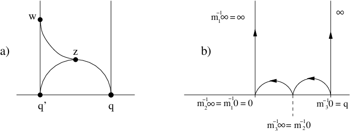
Figure 1b gives an illustration of the paths $\bigcup_{l=1}^{3}L_{m_{l}^{-1}0,m_{l}^{-1}\infty}$ and $L_{q,\infty}$ .

Refer to caption — Figure 1: Diagram (a) illustrates the paths used in the proof of Lemma 5.3. Diagram (b) illustrates the paths $L_{q,\infty}$ and $\bigcup_{l}L_{m_{l}^{-1}0,m_{l}^{-1}\infty}$ for e.g. $q=\frac{2}{3}$ .

Lemma 5.2

Let $q$ , $L_{q,\infty}$ and $M(q)$ be as in Lemma 5.1. Both paths $L_{q,\infty}$ and $\bigcup_{l=1}^{L}L_{m_{l}^{-1}\,0,m_{l}^{-1}\,\infty}$ are in the first quadrant.

Proof. Obviously $L_{0,\infty}=\{it;t\geq 0\}$ and $L_{q,\infty}=\{q+it;t\geq 0\}$ ly in the first quadrant since $q\geq 0$ .

The construction of $M(q)$ gives $m_{l}^{-1}\,0=m_{l+1}^{-1}\,\infty\geq 0$ , $m_{1}^{-1}\,\infty=\infty$ and $m_{L}^{-1}\,0=q\geq 0$ . Hence the paths $L_{m_{l}^{-1}\,0,m_{l}^{-1}\,\infty}$ ly in the first quadrant. The lemma follows by composition of these paths. $\Box$

Lemma 5.3

For $\theta$ a closed $1$ -form on $\mathfrak{H}$ such that $\int_{L}\theta$ exists for all simple paths $L$ in $\mathfrak{H}^{\ast}$ we have

\int_{L_{q,\infty}}\theta=\int_{L_{q,q^{\prime}}}\theta+\int_{L_{q^{\prime},\infty}}\theta

for all $q,q^{\prime}\in\mathbb{Q}$ .

Proof. Choose points $z$ and $w\in\mathfrak{H}$ on the simple paths $L_{q,q^{\prime}}$ respectively $L_{q^{\prime},\infty}$ as illustrated in Figure 1a. We consider the simple paths $L^{1}=L_{q^{\prime},z}\cup L_{z,w}\cup L_{w,q^{\prime}}$ with simultanious initial and end point $q^{\prime}$ , $L^{2}$ with initial point $q$ and end point $\infty$ through the points $z$ and $w$ and $L^{3}$ with initial point $z$ and end point $\infty$ through the point $w$ .

We find that

\int_{L_{q,\infty}}\theta=\int_{L^{2}}\theta=\int_{L_{q,z}\cup L^{3}}\theta=\int_{L_{q,z}}\theta+\int_{L^{3}}\theta

since $\theta$ is closed and composition $L^{2}=L_{q,z}\cup L^{3}$ . Moreover $\int_{L^{1}}\theta$ vanishes. Hence we have

$\displaystyle\int_{L_{q,\infty}}\theta$	$\displaystyle=$	$\displaystyle\int_{L_{q,z}}\theta+\int_{L^{1}}\theta+\int_{L^{3}}\theta$
	$\displaystyle=$	$\displaystyle\int_{L_{q,z}}\theta+\int_{L_{z,w}}\theta+\int_{L_{w,q^{\prime}}}\theta+\int_{L_{q^{\prime},z}}\theta+\int_{L^{3}}\theta$
	$\displaystyle=$	$\displaystyle\int_{L_{q,q^{\prime}}}\theta+\int_{L_{q^{\prime},\infty}}\theta.$

$\Box$

We will show in this section how the Hecke operators $H_{m}$ induce operators $\tilde{H}_{m}$ on period functions.

Lemma 5.4

Let $u\in S(1,s)$ be a cusp form and $Pu$ the period function as in Definition 4.2. For $A={\textstyle\left({\ast\atop 0}\>{\ast\atop d}\right)}\in X_{m}$ and $M(A0)=\sum_{l=1}^{L}m_{l}\in\mathcal{R}_{1}$ we have

m^{s}d^{-2s}\,\int_{L_{A0,A\infty}}\eta\big(u,R_{A\zeta}^{s}\big)=\sum_{l=1}^{L}\big(Pu\big|_{s}m_{l}A\big)(\zeta)=\big(Pu\big|_{s}M(A0)A\big)(\zeta)

(32)

for all $\zeta>0$ .

Proof. For $l\in\{1,\ldots,L\}$ we find

\int_{L_{m_{l}^{-1}0,m_{l}^{-1}\infty}}\eta\big(u,R_{A\zeta}^{s}\big)=\int_{L_{0,\infty}}\eta\big(u\big|_{0}m_{l}^{-1},R_{A\zeta}^{s}\big|_{0}m_{l}^{-1}\big)

using Lemma 4.1. Since $m_{l}^{-1}\in{\Gamma(1)}$ and $u$ is a cusp form one has $u\big|_{0}m_{l}^{-1}=u$ . Using (21) we find for $m_{l}={\textstyle\left({\ast\atop c_{l}}\>{\ast\atop d_{l}}\right)}$

R_{A\zeta}^{s}\big|_{0}m_{l}^{-1}=(c_{l}A\zeta+d_{l})^{-2s}\,R_{m_{l}A\zeta}^{s}\big|_{0}m_{l}m_{l}^{-1}=(c_{l}A\zeta+d_{l})^{-2s}\,R_{m_{l}A\zeta}^{s}.

The expression $(c_{l}A\zeta+d_{l})^{-2s}$ is well defined since $c_{l}A\zeta+d_{l}>0$ (see Lemma 2.9).

Recall that $A={\textstyle\left({\ast\atop 0}\>{\ast\atop d}\right)}$ and $\det A=m$ . We have

	$\displaystyle m^{s}d^{-2s}\,\int_{L_{m_{l}^{-1}0,m_{l}^{-1}\infty}}\eta\big(u,R_{A\zeta}^{s}\big)$
	$\displaystyle\quad=\,m^{s}d^{-2s}(c_{l}A\zeta+d_{l})^{-2s}\,\int_{L_{0,\infty}}\eta\big(u,R_{m_{l}A\zeta}^{s}\big)$
	$\displaystyle\quad=\,\big(Pu\big\|_{s}m_{l}A\big)(\zeta).$

Since Lemma 2.10 shows $m_{l}A\in\mathrm{Mat}_{m}^{+}(2,\mathbb{Z})$ , condition (b) in §1 holds and the slash action above is well defined.

On the other hand consider the term $\int_{L_{m_{L}^{-1}0,\infty}}\eta\big(u,R_{A\zeta}^{s}\big)$ . Lemma 5.3 implies that

\int_{L_{m_{L}^{-1}0,\infty}}\eta\big(u,R_{A\zeta}^{s}\big)=\int_{L_{m_{L}^{-1}0,m_{L}^{-1}\infty}}\eta\big(u,R_{A\zeta}^{s}\big)+\int_{L_{m_{L-1}^{-1}0,\infty}}\eta\big(u,R_{A\zeta}^{s}\big)

since the matrices $m_{l}$ satisfy (31). Iterating the argument gives

\int_{L_{m_{L}^{-1}0,\infty}}\eta\big(u,R_{A\zeta}^{s}\big)=\sum_{l=1}^{L}\int_{L_{m_{l}^{-1}0,m_{l}^{-1}\infty}}\eta\big(u,R_{A\zeta}^{s}\big).

Since $L_{A0,A\infty}=L_{m_{L}^{-1}0,\infty}$ we find

m^{s}d^{-2s}\,\int_{L_{A0,A\infty}}\eta\big(u,R_{A\zeta}^{s}\big)=\sum_{l=1}^{L}\big(Pu\big|_{s}m_{l}A\big)(\zeta)

for $\zeta>0$ . $\Box$

Now, we can define linear operators $\tilde{H}_{m}$ on period functions.

Definition 5.5

For $m\in\mathbb{N}$ define $\tilde{H}(m)\in\mathcal{R}_{m}$ as

\tilde{H}(m)=\sum_{d|m\atop 0\leq b<d}M\big({\textstyle\frac{b}{d}}\big){\textstyle\left({\frac{m}{d}\atop 0}\>{b\atop d}\right)}.

(33)

For $s\in\mathbb{C}$ the formal sum $\tilde{H}(m)$ induces an operator $\tilde{H}_{m}$ on the space of holomorphic functions on $(0,\infty)$ through

\tilde{H}_{m}f=f\big|_{s}\tilde{H}(m)\qquad(f\in C^{\omega}(0,\infty)).

(34)

Remark. The matrices in the formal sum $\tilde{H}(m)$ in (33) have only nonnegative integer entries as shown in Lemma 2.10. Hence $f\big|_{s}\tilde{H}(m)(\zeta)$ in (34) is well defined for all $\zeta>0$ .

Lemma 2.11 implies that the set

\{m_{l}A;\,A\in X_{m},\,M(A0)=\sum_{l=1}^{L}m_{l}\},

which contains all matrices appearing in the formal sum $\tilde{H}(m)$ , is a subset of

S_{m}=\left\{{\textstyle\left({a\atop c}\>{b\atop d}\right)};\,a>c\geq 0,d>b\geq 0\right\}\subset\mathrm{Mat}_{n}^{+}(2,\mathbb{Z}).

It is shown in [HMM05] that both sets are indeed equal. (The authors in [HMM05] assume that $\gcd(a,b,c,d)=1$ but this restriction is not necessary.) Hence $\tilde{H}(m)\in\mathcal{R}_{m}^{+}$ is given by $\tilde{H}(m)=\sum_{B\in S_{m}}B$ .

Lemma 5.6

Let $Pu$ be the period function of the cusp form $u\in S(1,s)$ . For any $m\in\mathbb{N}$ the operator $\tilde{H}_{m}$ satisfies

\Big(\tilde{H}_{m}(Pu)\Big)(\zeta)=\int_{0}^{i\infty}\eta\big(H_{m}u,R_{\zeta}^{s}\big)\qquad\mbox{for }\zeta>0.

(35)

Proof. Let $Pu$ be the period function of $u\in S(1,s)$ . Let $H_{m}$ be the Hecke operator in (6). For $A={\textstyle\left({a\atop 0}\>{b\atop d}\right)}\in X_{m}$ we have using Lemma 4.1 and Equation (21)

	$\displaystyle\int_{L_{0,\infty}}\eta\big(u\big\|_{0}A,R_{\zeta}^{s}\big)$	$\displaystyle=$	$\displaystyle\int_{L_{A0,A\infty}}\eta\left(u,(R_{\zeta}^{s}\big\|_{0}A^{-1})\right)$
		$\displaystyle=$	$\displaystyle\left(\frac{\det A}{d^{2}}\right)^{s}\,\int_{L_{A0,A\infty}}\eta\big(u,R_{A\zeta}^{s}\big).$

Applying Lemma 5.4 we find

\int_{L_{0,\infty}}\eta\big(u\big|_{0}A,R_{\zeta}^{s}\big)=\big(Pu\big|_{s}M(A0)A\big)(\zeta).

Next we can compute $\int_{L_{0,\infty}}\eta\big(H_{m}u,R_{\zeta}^{s}\big)$ for $H_{m}u$ in (6) and find

\int_{L_{0,\infty}}\eta\big(H_{m}u,R_{\zeta}^{s}\big)=\sum_{A\in X_{m}}\Big(Pu\big|_{s}M\left(A0\right)A\Big)(\zeta)=Pu\big|_{s}\tilde{H}(m)(\zeta)

since $\tilde{H}(m)=\sum_{A\in X_{m}}M(A0)A$ . $\Box$

Proposition 5.7

For $u\in S(1,s)$ the period function $Pu\in\mathrm{FE}(1,s)$ satisfies the identity

\big(Pu\big)\big|_{s}\tilde{H}(m)=P\big(u\big|_{0}H(m)\big).

Proof. This follows immediately from Lemma 5.6. $\Box$

Remark. Proposition 5.7 shows how the Hecke operators $H_{m}$ on cusp forms for ${\Gamma(1)}$ induce Hecke operators on period functions for this group. These Hecke operators are the same as the operators in [HMM05]. The authors of [HMM05] derived the operators using only period functions respectively transfer operators for the groups ${\Gamma_{0}\left(m\right)}$ . Another derivation of $\tilde{H}_{m}$ for ${\Gamma(1)}$ is given also in [Mu04] using a criterion found by Choie and Zagier in [CZ93]. A similar representation of the Hecke operators has been given by L. Merel in [Me94].

5.2 Hecke operators for period functions for ${\Gamma_{0}\left(n\right)}$

In this section we extend the above derivation of the Hecke operators for period functions for ${\Gamma(1)}$ to the congruence subgroups ${\Gamma_{0}\left(n\right)}$ .

Lemma 5.8

For $A={\textstyle\left({\ast\atop 0}\>{\ast\atop d}\right)}\in X_{m}$ put $M(A0)=\sum_{l=1}^{L}m_{l}\in\mathcal{R}_{1}$ . If $P\vec{u}$ is a period function of $\vec{u}\in S_{\mathrm{ind}}(n,s)$ , then

m^{s}d^{-2s}\,\int_{L_{A0,A\infty}}\eta\big(\vec{u},R_{A\zeta}^{s}\big)=\sum_{l=1}^{L}\rho(m_{l}^{-1})\,\Big(P\vec{u}\big|_{s}m_{l}A\Big)(\zeta)\qquad\mbox{for }\zeta>0.

(36)

Proof. Using the transformation property of $\eta$ in Lemma 4.1 we get for $l\in\{1,\ldots,L\}$

\int_{L_{m_{l}^{-1}0,m_{l}^{-1}\infty}}\eta\big(\vec{u},R_{A\zeta}^{s}\big)=\int_{L_{0,\infty}}\eta\big(\vec{u}\big|_{0}m_{l}^{-1},R_{A\zeta}^{s}(m_{l}^{-1}\cdot)\big).

An argument as in the proof of Lemma 5.4 gives

R_{A\zeta}^{s}\big|_{0}m_{l}^{-1}=(c_{l}A\zeta+d_{l})^{-2s}\,R_{m_{l}A\zeta}^{s}(m_{l}m_{l}^{-1}\cdot)=(c_{l}A\zeta+d_{l})^{-2s}\,R_{m_{l}A\zeta}^{s}

if $m_{l}={\textstyle\left({\ast\atop c_{l}}\>{\ast\atop d_{l}}\right)}$ . Since $c_{l}A\zeta+d_{l}>0$ the expression $(c_{l}A\zeta+d_{l})^{-2s}$ is well defined.

Using $\vec{u}\big|_{0}m_{l}^{-1}=\rho(m_{l}^{-1})\vec{u}$ for $m_{l}^{-1}\in{\Gamma(1)}$ we find

	$\displaystyle m^{s}d^{-2s}\,\int_{L_{m_{l}^{-1}0,m_{l}^{-1}\infty}}\eta\big(\vec{u},R_{A\zeta}^{s}\big)$
	$\displaystyle\quad=\,m^{s}d^{-2s}(c_{l}A\zeta+d_{l})^{-2s}\,\rho(m_{l}^{-1})\,\int_{L_{0,\infty}}\eta\big(\vec{u},R_{m_{l}A\zeta}^{s}\big)$
	$\displaystyle\quad=\,\rho(m_{l}^{-1})\,\Big(P\vec{u}\big\|_{s}m_{l}A\Big)(\zeta).$

Consider $\int_{L_{A0,A\infty}}\eta\big(\vec{u},R_{A\zeta}^{s}\big)(z)$ . The same argument as in the proof of Lemma 5.4 shows

\int_{L_{A0,A\infty}}\eta\big(\vec{u},R_{A\zeta}^{s}\big)=\sum_{l=1}^{L}\int_{L_{m_{l}^{-1}0,m_{l}^{-1}\infty}}\eta\big(\vec{u},R_{A\zeta}^{s}\big).

But this gives

m^{s}d^{-2s}\,\int_{L_{A0,A\infty}}\eta\big(\vec{u},R_{A\zeta}^{s}\big)=\sum_{l=1}^{L}\rho(m_{l}^{-1})\,\big(P\vec{u}\big|_{s}m_{l}A\big)(\zeta).

$\Box$

For $n=1$ Lemma 5.8 is just Lemma 5.4 since $\rho$ is trivial in this case.

In the following we denote the $i^{\mathrm{th}}$ component of the vector $\vec{u}$ by $[\vec{u}]_{i}$ .

Lemma 5.9

Let $\alpha_{1},\ldots,\alpha_{\mu}$ be representatives of the right coset of ${\Gamma_{0}\left(n\right)}$ in ${\Gamma(1)}$ where $\mu=[{\Gamma(1)}:{\Gamma_{0}\left(n\right)}]$ . Let $P\vec{u}$ be the period function of $\vec{u}\in S_{\mathrm{ind}}(n,s)$ . For $A\in X_{m}$ , $j\in\{1,\ldots,\mu_{n}\}$ let be $M(\sigma_{\alpha_{j}}(A)0)=\sum_{l=1}^{L}m_{l}\in\mathcal{R}_{1}$ . Then the following identity holds for all $j\in\{1,\ldots,\mu\}$ and $\zeta>0$ :

\int_{L_{0,\infty}}\eta\big([\vec{u}]_{\phi_{A}(j)}\big|_{0}\sigma_{\alpha_{j}}(A),R_{\zeta}^{s}\big)=\sum_{l=1}^{L}\left[\rho(m_{l}^{-1})\,P\vec{u}\right]_{\phi_{A}(j)}\big|_{s}m_{l}\sigma_{\alpha_{j}}(A)\,(\zeta).

(37)

Proof. Write $\vec{u}=(u_{j})_{j}$ . Using Lemma 4.1 and property (21) of $R_{\zeta}$ we find for any $j\in\{1,\ldots,\mu_{n}\}$ and $\zeta>0$ :

	$\displaystyle\int_{L_{0,\infty}}\eta\big(u_{\phi_{A}(j)}\big\|_{0}\sigma_{\alpha_{j}}(A),R_{\zeta}^{s}\big)\,=\,\int_{L_{\sigma_{\alpha_{j}}(A)0,\sigma_{\alpha_{j}}(A)\infty}}\eta\big(u_{\phi_{A}(j)},R_{\zeta}^{s}\big\|_{0}\big(\sigma_{\alpha_{j}}(A)\big)^{-1}\big)$
	$\displaystyle\quad=\,m^{s}d_{j}^{-2s}\,\int_{L_{\sigma_{\alpha_{j}}(A)0,\sigma_{\alpha_{j}}(A)\infty}}\eta\Big(u_{\phi_{A}(j)},R_{\sigma_{\alpha_{j}}(A)\zeta}^{s}\Big)$

where $\sigma_{\alpha_{j}}(A)={\textstyle\left({\ast\atop 0}\>{\ast\atop d_{j}}\right)}$ is again in $X_{m}$ . Take $M(\sigma_{\alpha_{j}}(A)0)=\sum_{l=1}^{L}m_{l}\in\mathcal{R}_{1}$ and apply Lemma 5.8. We have

	$\displaystyle\int_{L_{0,\infty}}\eta\big(u_{\phi_{A}(j)}\big\|_{0}\sigma_{\alpha_{j}}(A),R_{\zeta}^{s}\big)$	$\displaystyle=$	$\displaystyle\Big[\int_{L_{0,\infty}}\eta\big(\vec{u}\big\|_{0}\sigma_{\alpha_{j}}(A),R_{\zeta}^{s}\big)\Big]_{\phi_{A}(j)}$
		$\displaystyle=$	$\displaystyle\left[\sum_{l=1}^{L}\rho(m_{l}^{-1})\,\Big(P\vec{u}\Big\|_{s}m_{l}\sigma_{\alpha_{j}}(A)\Big)(\zeta)\right]_{\phi_{A}(j)}.$

$\Box$

Remark. For $u\in S(n,s)$ and $A\in X_{m}$ Lemma 3.5 implies that

u\big|_{0}A\alpha_{j}=u\big|_{0}\alpha_{\phi_{A}(j)}\sigma_{\alpha_{j}}(A).

Hence equation (37) can be written as

\int_{L_{0,\infty}}\eta\big(\Pi(u\big|_{0}A),R_{\zeta}^{s}\big)=\sum_{l=1}^{L}\left[\rho(m_{l}^{-1})\,P\Pi(u)\right]_{\phi_{A}(j)}\big|_{s}m_{l}\sigma_{\alpha_{j}}(A)\,(\zeta)

Lemma 5.9 allows us to derive an explicit formula for the action of the Hecke operators on the period functions of ${\Gamma_{0}\left(n\right)}$ induced from the action of these operators on $S_{\mathrm{ind}}(n,s)$ for this group.

Proposition 5.10

Let $\alpha_{1},\ldots,\alpha_{\mu}$ be representatives of the right cosets of ${\Gamma_{0}\left(n\right)}$ in ${\Gamma(1)}$ . Let $P\vec{u}$ be the period function of $\vec{u}\in S_{\mathrm{ind}}(n,s)$ . For $m$ prime take $\mathbf{A}\subset X_{m}$ such that $T(m)=\sum_{A\in\mathbf{A}}A$ if $\gcd(m,n)=1$ resp. $U(m)=\sum_{A\in\mathbf{A}}A$ if $m|n$ . The $m^{\mathrm{th}}$ Hecke operator $\tilde{H}_{n,m}$ acting on $P\vec{u}$ is given by

\left[\tilde{H}_{n,m}\big(P\vec{u}\big)\right]_{j}=\sum_{A\in\mathbf{A}}\sum_{l=1}^{L}\left[\rho(m_{l}^{-1})\,P\vec{u}\right]_{\phi_{A}(j)}\big|_{s}\big(m_{l}\sigma_{\alpha_{j}}(A)\big).

(38)

Remark. We emphasize that the constant $L$ in (38) depends on $A$ and that $\mathbf{A}=X_{m}$ for $\gcd(m,n)=1$ resp. $\mathbf{A}=X_{m}\smallsetminus\left\{{\textstyle\left({m\atop 0}\>{0\atop 1}\right)}\right\}$ for $m|n$ .

Proof of Proposition 5.10. The $m^{\mathrm{th}}$ Hecke operator $H_{n,m}$ acts on $\vec{u}$ as

\left[H_{n,m}\vec{u}\right]_{j}=\sum_{A}\,u_{\phi_{A}(j)}\big|_{0}\sigma_{\alpha_{j}}(A)\qquad\mbox{for }k\in\{1,\ldots,\mu\}.

Applying Lemma 5.9 to both sides then gives formula (38). $\Box$

Acknowledgments. This work has been supported by the Deutsche Forschungsgemeinschaft through the DFG Forschergruppe “Zetafunktionen und lokalsymmetrische Räume”. The author thanks Dieter Mayer and Joachim Hilgert for their discussions and comments.

References

[AS65] M. Abramowitz an d I. A. Stegun. Handbook of mathematical functions Dover Publications, Inc., 1965.
[AL70] A. O. L. Atkin and J. Lehner. Hecke operators on $\Gamma_{0}(m)$ . Math. Ann. 185 (1970) 134 – 160.
[Br94] R. W. Bruggeman. Families of Automorphic forms, volume 88 in Monographs in Mathematics Birkhäuser Verlag, 1994.
[Ch99] C.-H. Chang. Die Transferoperator-Methode für Quantenchaos auf den Modulflächen $\Gamma\backslash\mathbb{H}$ . PhD thesis, Mathematisch-Naturwissenschaftliche Fakultät der Technischen Universität Clausthal, Januar 1999.
[CZ93] Y. J. Choie and D. Zagier. Rational period functions for $\mathrm{PSL}(2,\mathbb{Z})$ . In M. Knopp and M. Sheingorn, editors, A Tribune to Emil Grosswald: Number Theory and related Analysis, volume 143 of Contemporary Mathematics, pages 89–108. American Mathematical Society, 1993.
[DH04] A. Deitmar and J. Hilgert. The Lewis Correspondence for submodular groups. e-arxiv, 2004. http://arXiv.org/abs/math/0404067.
[HMM05] J. Hilgert, D. Mayer and H. Movasati. Transfer operators for $\Gamma_{0}(n)$ and the Hecke operators for period functions of $\mathrm{PSL}(2,\mathbb{Z})$ . To appear in Math. Proc. Camb. Phil. Soc. (2005).
[Hu94] A. Hurwitz. Ueber die angenäherte Darstellung der Zahlen durch rational Brüche. Mathematische Annalen 44 (1894) 417–436.
[Iw02] H. Iwaniec. Spectral Methods of Automorphic Forms, volume 53 of Graduate Studies in Math. American Mathematical Society, 2002.
[La76] S. Lang. Introduction to modular forms, volume 222 of Grundl. math. Wiss. Springer Verlag, Berlin, 1976.
[LZ01] J. Lewis and D. Zagier. Period functions for Maass wave forms. I. Ann. of Math. 153 (2001) 191–258.
[Ma01] F. Martin. Périodes de formes modularires de poids 1, Thèse doctorate, Paris 7, 2001.
[MM] D. Mayer and T. Mühlenbruch. From the transfer operator for geodesic flows on modular surfaces to the Hecke operators on period functions of $\Gamma_{0}(n)$ , In Dynamical Systems: from Algebraic to Topoligical Dynamics. Proccedings of the ESF-Exploratory Workshop, 5-9 July 2004, Bonn. To appear in Contemporary Mathematics, American Mathematical Society.
[Me94] L. Merel. Universal Fourier expansions of modular forms. In G. Frey, editor, On Artkins conjecture for odd $2$ -dimensional representations, volume 1585 of Lecture Notes in Math. Springer Verlag, Berlin, 1994.
[Mi89] T. Miyake. Modular Forms. Springer-Verlag, 1989.
[Mü03] T. Mühlenbruch. Systems of automorphic forms and period functions. PhD thesis, Utrecht University, September 2003.
[Mu04] T. Mühlenbruch. Hecke operators on period functions for the full modular group. IMRN 4127-4145 (2004).

Tobias Mühlenbruch
Institut für Theoretische Physik
Abteilung Statistische Physik und Nichtlineare Dynamik
Technische Universität Clausthal
Arnold-Sommerfeld-Straße 6
38678 Clausthal-Zellerfeld
Germany
email: tobias.muehlenbruch@tu-clausthal.de

	$\displaystyle\int_{L_{0,\infty}}\eta\big(u_{\phi_{A}(j)}\big\|_{0}\sigma_{\alpha_{j}}(A),R_{\zeta}^{s}\big)$	$\displaystyle=$	$\displaystyle\Big[\int_{L_{0,\infty}}\eta\big(\vec{u}\big\|_{0}\sigma_{\alpha_{j}}(A),R_{\zeta}^{s}\big)\Big]_{\phi_{A}(j)}$
		$\displaystyle=$	$\displaystyle\left[\sum_{l=1}^{L}\rho(m_{l}^{-1})\,\Big(P\vec{u}\Big\|_{s}m_{l}\sigma_{\alpha_{j}}(A)\Big)(\zeta)\right]_{\phi_{A}(j)}.$

Hecke operators on period functions for Γ0​(n)\Gamma_{0}(n)

Abstract

1 Introduction

2 On Farey sequences

2.1 Farey sequences a la Hurwitz

Definition 2.1

Lemma 2.2

Lemma 2.3

2.2 Left neighbor sequences

Lemma 2.4

Definition 2.5

Lemma 2.6

Lemma 2.7

Definition 2.8

Lemma 2.9

Lemma 2.10

Lemma 2.11

3 Vector valued cusp forms and Hecke operators

3.1 Hecke operators for scalar valued cusp forms

Definition 3.1

3.2 Induced representations

3.3 Vector valued cusp forms

Definition 3.2

Lemma 3.3

Lemma 3.4

3.4 Hecke operators for cusp forms

Lemma 3.5

Lemma 3.6

Definition 3.7

Definition 3.8

Proposition 3.9

4 On period functions

4.1 Some technical computations

Lemma 4.1

4.2 The period functions of vector valued cusp forms

Definition 4.2

Lemma 4.3

Lemma 4.4

Proposition 4.5

Proposition 4.6

5 Main result

5.1 Hecke operators for period functions for Γ⁡(1){\Gamma(1)}

Lemma 5.1

Lemma 5.2

Lemma 5.3

Lemma 5.4

Definition 5.5

Lemma 5.6

Proposition 5.7

5.2 Hecke operators for period functions for Γ0​(n){\Gamma_{0}\left(n\right)}

Lemma 5.8

Lemma 5.9

Proposition 5.10

References

Hecke operators on period functions for $\Gamma_{0}(n)$

5.1 Hecke operators for period functions for ${\Gamma(1)}$

5.2 Hecke operators for period functions for ${\Gamma_{0}\left(n\right)}$