Time-Dependent Solutions of a Discrete Schrödinger’s Equation
Time-Dependent Solutions of a Discrete Schrödinger’s Equation
By
NIGIE SHI
B.S. (University of Wyoming) 2001
THESIS
Submitted in partial satisfaction of the requirements for the degree of
MASTER OF SCIENCE
in
APPLIED MATHEMATICS
in the
OFFICE OF GRADUATE STUDIES
of the
UNIVERSITY OF CALIFORNIA,
DAVIS
Approved:
Committee in Charge
2004
Acknowledgments
I would like to thank for Professor Bruno Nachtergaele for giving me this interesting project and being my thesis advisor and Professor Albert C. Fannjiang and Professor Alexander Soshnikov who are working in related fields for kindly agreeing to be members of my thesis committee and review my thesis. I especially like to show my great appreciation to Professor Bruno Nachtergaele’s patient guidance for helping me complete this project. The process is very invaluable. Professor Albert C. Fannjiang and Professor Alexander Soshnikov are also my instructors for the two graduate preliminary math courses MAT 119 and MAT 203, respectively. I have learned a lot from them during my first year of graduate study at Uuniversity of California, Davis. Also, I would like to thank for Arthur Cheng, Jeremy Clark, Ben-Shan Liao, and Yuan-Kai Huang who are my colleagues for consulting related materials of my project in both analysis and numerics.
Moreover, mathematics is always my primary interest including researching and teaching that I would like to work on both of them for my future career and I sincerely appreciate Professor Bruno Nachtergaele, Professor Alex Mogilner, Professor Elbridge Gerry Puckett, Doctor Duane Kouba, and Professor Jim Diederich for writing my letters of recommendation.
Finally, I would like to thank for my parents Mei-Pin Shi and Ling-Ju Lin of supporting me to come to United States of America for my college education at University of Wyoming. Based on my hard work during undergraduate and their constant encouragement, I am able to go to University of California, Davis for my graduate study.
1. Introduction
A very useful method of studying linear operators by decomposing the space on which they act into invariant subspaces is known as spectral theory. An example of an application of spectral theory is the problem of finding a set of eigenvectors or diagonalizing a linear map on an infinite-dimensional space [HN]. When a finite dimensional linear operator is diagonalized, there exist a set of eigenvalues and their corresponding eigenvectors. Along the directions of an eigenvector with its given eigenvalue, the action of the operator is just multiplication by the eigenvalue. The spectrum contains the set of eigenvalues that is also called point spectrum. In infinite dimensional case, the structure of the spectrum will often be more complicated such that there may exist a continuous spectrum or residual spectrum which do not contain a set of eigenvalues and are different from the point spectrum. In my thesis, I study the spectrum of an operator based on some numerical results of it and also properties of the discrete Laplacian operator.
The discrete Laplacian operator is defined on by
where . Moreover, three features of are described in a theorem as follows:
Theorem 1.
Let be the right shift operator and be the left shift operator. . The spectrum of is entirely continuous and consists of the interval .
Proof. First, where denotes the operator norm. Second, . These two arguments imply that where denotes the spectrum of . The facts that and is purely continuous will be shown in Section 3.
The discrete Laplacian operator is one of the most important and oldest difference operator [D] which is closely related to the operator I’m studying in this paper. But before I introduce this operator, I would like to talk about Schrödinger’s equation and Schrödinger operators.
A Schrödinger’s equation without a potential term is a partial differential equation defined as [E]. On the other hand, Schrödinger operators acting on are operators such as , where is a real-valued function on and is called a potential [D]. We may impose condition on such as choosing so that is an self-adjoint operator on . For a detailed proof of this specific condition, see Davies [D]. Moreover, ‘ with is called a wave packet or state, and represents the instantaneous configuration of a collection of electrons, atoms and molecules. The operator is also called the Hamiltonian for historical reasons - quantum theory can be regraded as a non-commutative version of classical Hamiltonian mechanics. The evolution of a quantum system is controlled by the Schrödinger’s equation with solution ’ [D].
Finally, I want to now introduce the problem of my project. The term ‘’ which you will see below is a coefficient, not the discrete Laplacian operator mentioned above.
For a particular example of a Schrödinger’s equation which is also the main subject of my thesis, a time-dependent discrete Schrödinger’s equation defined on can be written as follows:
where
with , , , .
In order to understand the operator , we define and study as follows
such that
is linear and bounded. The fact that is linear is trivial. is bounded because since the maxima of and are and , respectively. The reason that the maximum of is for any and is because of the properties of which will explained in Section 2, and also Figure 1 below plots an example of versus .
As you can see that the two main differences between the discrete Laplacian operator and are the tridiagonal terms of their matrices where those terms in the discrete Laplacian operator are constant functions: , , and those in are variables depending on and : , , respectively.
We know that the spectrum of the discrete Laplacian operator contains only the continuous spectrum when the diagonal terms of the operator are constants . On the other side, the diagonal terms of the operator have a trapping region around their centers and are for large . Figure 1 presented below shows an example of with certain parameters and . So, is a perturbed case of the discrete Laplacian operator, and the nature of the structure of the spectrum of is different from it of the discrete Laplacian operator because of the term .

In this paper, I study the spectrum of defined above based on the discrete Laplacian operator which is an unperturbed case of and also some numerical results that can be used to investigate the solutions of the time-dependent discrete Schrödinger’s equation from the following three aspects:
- •
stationary solution ()
- •
periodic solution ()
- •
properties or representatives of the general solution
I have only studied the stationary and periodic solutions but not yet the properties or representatives of general solution here.
For infinite dimensional depending on and , my research shows that there exist three eigenvalues depending on a certain region of and . The first eigenvalue of which equals zero is exact. A detailed analysis regrading this eigenvalue also called the zero mode [MN] will be discussed in Section 3. Moreover, a second eigenvalue exists which is proved by Michoel and Nachtergaele [MN]. Finally, we also predict that a third eigenvalue exists for certain parameters and based my numerical results. The primary focus in my thesis is to find critical values or intervals of the parameters and where these eigenvalues exist by numerics. More precisely, the main object is to determine the particular regions where there exist one, two, or three eigenvalues for infinite dimensional . In order to study this operator by numerics, we concentrate on a finite dimensional subspace of such that is a finite dimensional operator. Since there always exists a set of eigenvalues for finite dimensional , we therefore focus on the eigenvalues that are isolated from the set of all other eigenvalues which will belong to the continuous spectrum and consider those isolated ones as the candidates of eigenvalues which will belong to the point spectrum for infinite dimensional . Those ‘isolated eigenvalues’ I mentioned can be seen more clearly on Figure 3 and Figure 4 in Section 3.
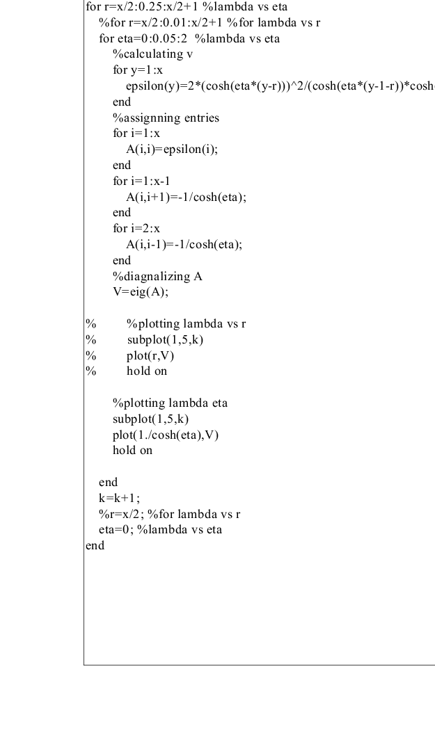
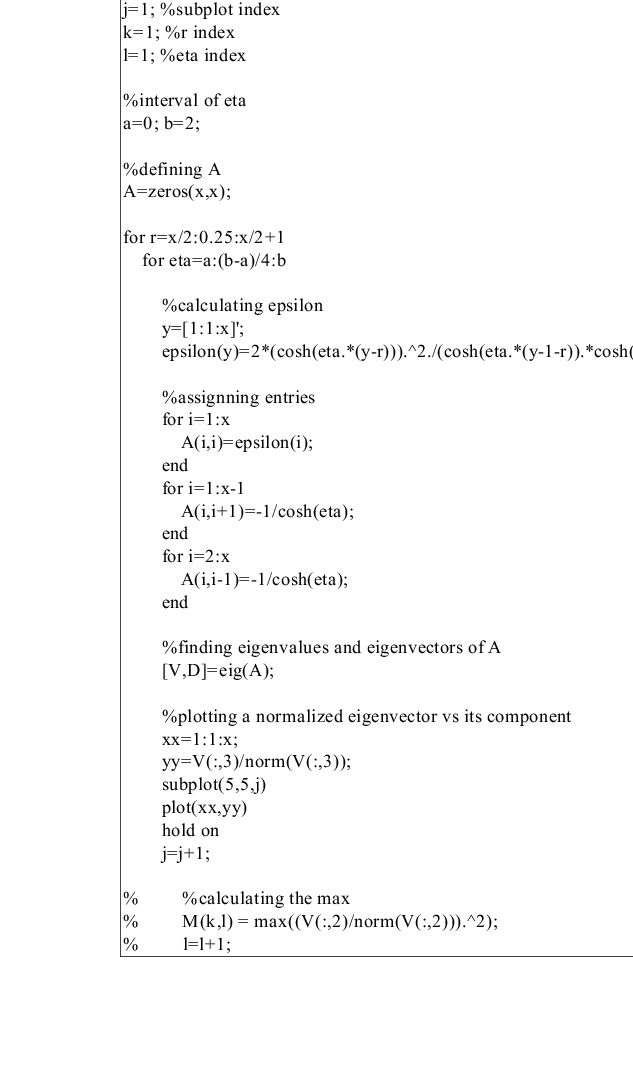
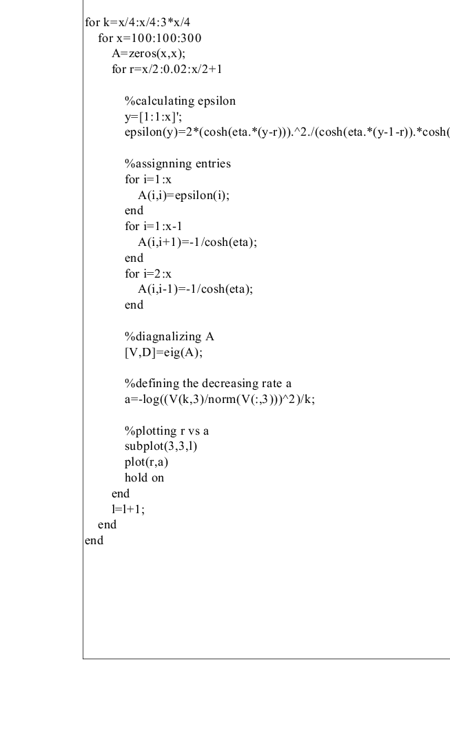
My numerical results are created by three programs written by myself in MATLAB. First, I graph the spectrum of versus both parameters and separately to see how the set of the point spectrum is distributed with different and . Second, I graph the eigenvectors with respect to the three eigenvalues versus their components to see how the eigenvectors are distributed and I’m hoping to see that the eigenvectors are still nonzero for large matrix size with certain and . Third, I calculate the maxima of the square normalized components of all those three eigenvectors. I compare the maxima with the same parameters and different matrix sizes individually and my expectation is that if the maxima do not decrease at certain values or intervals of and , then the eigenvectors are not zero which also implies that there exist eigenvalues for infinite dimensional . This step mainly support my results. Finally, for the third eigenvalue mentioned above, I also observe three components of its corresponding eigenvector to see the decreasing rates of them. My meaning of decreasing rates will be explained in the next few sections. This process is to determine whether my conclusion of the existence of the third eigenvalue at certain and based on the previous steps are correct or not. The next three sections show my analysis in detail of the problem and the last section concludes my entire paper, and they are presented in the order as follows:
- Primary Results:
-
This section states the procedures and the main discoveries in my project.
- The Spectrum:
-
This section discusses the definition of spectrum and also the structure and feature of the spectrum of .
- The Eigenvalues:
-
This section shows my numerical results for all the eigenvalues that are found.
- Conclusion:
-
This section summarizes my results and also talks about some further discussions of this operator.
2. Preliminary Results
If is a finite dimensional operator, then it is also a compact operator. A compact operator is bounded, and a compact operator that is also symmetric is self-adjoint. For more details, see Hunter and Nachtergaele [HN]. Therefore, is a self-adjoint operator. Moreover, is a nonnegative operator. In order to prove this fact, we need to use the following lemma first.
Lemma 1.
Let be a matrix such that
where , . Then if and only if and .
Proof. Let . First, if and only if all its eigenvalues . Second, the determinant of after simplification is . Moreover,
Since , we have and . Conversely, if and , then which also implies that .
Now, we can decompose into infinitely many submatrices such that where
because where
Since only four entries in are nonzero, if we want to prove that is nonnegative, it is sufficient to focus on a matrix defined as follows:
Since for all , and . Thus, the remaining is to show that whether is true or not. The calculation is presented below.
Hence, is nonnegative for all because and . So, is nonnegative for all which implies that is nonnegative and also all eigenvalues of are nonnegative.
For infinite dimensional , my numerical results predict that there exist three isolated eigenvalues of for a certain range of the parameters and such that the point spectrum of is not empty, unlike the discrete Laplacian operator. My conclusions are mainly based on calculating the maxima of the square normalized components of all the three eigenvectors corresponding to their eigenvalues with various and and also observe the pictures of all the three eigenvectors and the decreasing rates for three chosen elements of the eigenvector of the third eigenvalue to compare them with my numerics because the range of the existence of the third isolated eigenvalue with respect to and is different from it of the other two isolated eigenvalues. Roughly speaking, with certain interval of , the first two eigenvalues exist for all in a certain region which will be determined but the third eigenvalue does not exist for all in that region. More details are presented in the following few paragraphs.
I am using finite dimensional to approximate infinite dimensional . The reason why I follow such path is based on what we know about the discrete Laplacian operator. If , then is different from the discrete Laplacian operator only by a sign. Moreover, my numerical data includes the case where and it shows that the eigenvectors approach to zero when the size of becomes larger and larger though not presented here. So, we expect that all the eigenvectors of when converge to zero by the norm as the size of goes to infinity which indicates that the limits of the eigenvalues are in fact not eigenvalues. The reason that the converge is in the sense of norm is because my numerical data shows that the maxima of the square normalized components converge to zero, and so the convergence is also in the weak sense. Moreover, we already know that the spectrum of the discrete Laplacian operator does not contain any eigenvalue. Therefore, using finite cases of to predict infinite cases of is reliable even if we change the parameters and .
Now I want to talk about why I start with certain and out of other possibilities. For an n-dimensional where , the diagonal terms are exponentially localized functions. depends on and in which plays the role of shifting and concentrates around its center, and is also symmetric around its center shown in Figure 1 above. It is therefore sufficient to focus on the case where represents the size of . Moreover, is an even function because it is governed by hyperbolic cosine functions which are even. As a result, we can begin with and then gradually increase . By plotting the graphs for the set of eigenvalues of versus the parameter with increasing values of which will be displayed in the next section, the range of the set of the spectrum of becomes smaller and smaller and three isolated eigenvalues are extracted from the spectrum. For infinite dimensional case, these three eigenvalues will belong to the point spectrum and all others will belong to the continuous spectrum. The concept and structure of spectrum will also be discussed in the following section.
From my numerical results, there always exist two eigenvalues for all and . Moreover, for and , and for and , there exist a total of three eigenvalues. The graph shown below predicts the general results for the locations of the existence of the three isolated eigenvalues with different and for infinite approximation of . For numerical data which is not completely presented here, the third eigenvalue exists when and ; and ; and , and the two curves in the graph are produced based on connecting those points. More numerical results are therefore needed to verify this graph.

The results above show that the point spectrum of infinite dimensional is nonempty at these certain regions. Hunter and Nachtergaele [HN] and Michoel and Nachtergaele [MN] have proved the existence of the first and second isolated eigenvalues analytically, respectively. My results mainly come from comparing the maxima of the square components of normalized eigenvectors with different matrix size at certain values of and numerically. The idea is that when the maxima do not decrease for certain and while the matrix size becomes larger and larger, the eigenvalue does not vanish because its corresponding eigenvector is nonzero. More details of my numerical calculations of the results presented above will be discussed in the next two sections.
My numerical results including the maxima and the graphs of eigenvectors are created by a program written by myself in MATLAB named ”mainresults.m” and the one for observing the decreasing rates is called ”decreasingrates.m”. Also, the pictures of the spectrum of versus and , respectively, are generated by ”spectrum.m”. The purposes of these three programs will be explained in Section 3 and Section 4. The next section explains the spectrum of in more details and also discusses the spectrum of the discrete Laplacian operator.
3. The Spectrum
In some circumstances, there are no eigenvalues for an infinite dimensional bounded linear operator and so it is not possible to expect to find an orthonormal basis that consists entirely of eigenvectors. Thus, we need to define the spectrum in a more general way, instead of considering it only contains eigenvalues [HN].
The following two definitions are rewritten from ‘Applied Analysis’ by Hunter and Nachtergaele [HN].
Definition 1.
Let be a bounded operator defined on an infinite dimensional Hilbert space. The resolvent set of , denoted by , is the set of complex numbers such that is one-to-one and onto. The spectrum of , denoted by , is the complement of the resolvent set in , meaning that .
According to the open mapping theorem, is bounded if is one-to-to and onto, and therefore and are one-to-one, onto, bounded linear operators when . The following definition gives the structure of the spectrum of a bounded linear operator.
Definition 2.
Suppose that is a bounded linear operator on a Hilbert space.
- (1)
The point spectrum of consists of all such that is not one-to-one. In this case is called an eigenvalue of
- (2)
The continuous spectrum of consists of all such that is one-to-one but not onto, and the range of is dense in this Hilbert space.
- (3)
The residual spectrum of consists of all such that is one-to-one but not onto, and the range of is not dense in this Hilbert space.
We define on a finite subspace of for our problem and we then have where is an eigenvalue and is a nonzero eigenvector. Thus, the kernel of does not contain zero, and so is not one-to-one and .
Because of the diagonal term in , the structure of the spectrum of is different from it of the discrete Laplacian operator. As shown in Figure 1 above, the function remains constant for large but drops toward zero for small around its center. The existence of this dropping region makes the spectrum of so special in which the point spectrum is not empty such that we expect there exist eigenvalues when is infinite dimensional. The location, width, and depth of this trapping region depend significantly on the two parameters and .
Since is even and symmetric, shifts to the left or to the right depending on its sign, and concentrates narrow or wide around the center of depending on its magnitude, the most interesting case for is when the difference between and in is small. It is therefore sufficient to consider and where is the dimension of . Moreover, we can choose because is an even function.
The following five pictures plot the point spectrum or eigenvalues denoted them as of a finite versus with five different follows:

The first graph shows that the range of the spectrum of is in which is similar as the discrete Laplacian operator where it is in . The second graph shows that there is one isolated eigenvalue and the range of the other eigenvalues of is smaller than it when . The third graph where and the fourth graph where show that there are two isolated eigenvalues and the range of all the other eigenvalues becomes smaller and smaller even than before. At last, the fifth graph shows that there are three isolated eigenvalues and the range of the eigenvalues besides those three eigenvalues of is about [1.4,2.6]. However, at the third appearing eigenvalue seems to be still connecting with the spectrum, not totally isolated. Before I draw initial conclusions of critical values or intervals for and , I like to show another five pictures that plot the eigenvalues of versus where with five different as follows:

The first graph where and the fifth graph where show that there are three isolated eigenvalues at and two isolated eigenvalues at . corresponds approximately to and is about . Moreover, the second graph where and the fourth graph where show that there are still three isolated eigenvalues when and two isolated eigenvalues when , but now the third eigenvalue is not quite isolated from the set of other eigenvalues and seems to merge into the other sets of point spectrum. The third graph where show that there only exist two isolated eigenvalues. So, by Figure 3 and Figure 4 above, we can see that the third appearing eigenvalue does not seem to exist for all .
Therefore, we expect that the first and second isolated eigenvalues appear somewhere at and exist for all , and the third isolated eigenvalue appears somewhere at and exist for for all . By approximating infinite from finite , these three eigenvalues will remain in the point spectrum and all other eigenvalues will belong in the continuous spectrum.
You may ask that how numerical calculations for finite size systems can give insight in the infinite size systems. Since is defined on , we can focus on a subspace of such that is finite dimensional. Eigenvalues and eigenvectors of finite can be calculated by numerics and we can increase the size of since the eigenvectors are defined on . The spectrum of infinite dimensional can then be predicted by observing it of finite dimensional .
Moreover, we know the structure of the spectrum of the discrete Laplacian operator and is a perturbed case of it, we can study the spectrum of the discrete Laplacian operator in order to understand the spectrum of based on a theorem called the compact perturbation theorem below.
Theorem 2.
Let and let be . Then and have the same essential spectrum.
This theorem is rewritten from ‘Perturbation Theory for Linear Operators’ by Kato [K].
is constructed basically by reversing the sign of the discrete Laplacian operator and adding a compact perturbation term . The operator in is in fact a compact perturbation. To prove this statement, we can first define because we intend to show that is perturbed from which is the diagonal of the discrete Laplacian operator with inverse sign. We can then define an operator with finite-dimensional range such that is compact [HN] and
If , then is compact where denotes the operator norm. Now, we let and
So, because is as shown in Figure 1.
Thus, in is a compact perturbation and and the discrete Laplacian operator have the same essential spectrum. The spectrum of the discrete Laplacian operator is purely continuous and is contained in the interval and the point spectrum of finite at is contained in based on my numerics. When , is different from the discrete Laplacian operator by a sign. Moreover, my numerical results presented in the next section shows that at the maxima of the square normalized components of all the eigenvectors of the three isolated eigenvalues decrease as the matrix size of increase and we expect that the eigenvectors converge to zero for infinite . So, there are no eigenvalues when for infinite dimensional and they all converge to the set of the continuous spectrum. This fact agrees with the case of the discrete Laplacian operator. Therefore, when we change and of a finite n-dimensional , we expect that the three isolated eigenvalues will converge to the set of the point spectrum and all other eigenvalues will converge to the set of point spectrum as goes to infinity. Finally, the residual spectrum of the discrete Laplacian operator and are empty because they are both bounded and self-adjoint [HN].
The mathematical argument that determines the continuous spectrum in the infinite chain limit of the discrete Laplacian operator is presented below.
Let denote the Fourier transform and be the inverse Fourier transform. is an unitary operator. For proofs, see Hunter and Nachtergaele [HN]. Moreover, consider only now that is the discrete Laplacian operator.
It follows that where is a diagonal matrix that consists of spectral elements of on the diagonal since is self-adjoint. Moreover, if where and , then
It follows that and is entirely continuous.
Moreover, the bottom of the continuous spectrum of is given by a formula [MN] which agrees with my numerics shown in Figure 3 above. The smallest eigenvalue, or the first isolated eigenvalue of in our case, is also called the ”ground state energy” and its corresponding eigenfunction is called the ”ground state” which is the configuration of the system with the smallest total energy, and the other eigenvalues correspond to discrete excitations of the system [D].
As proved by Michoel and Nachtergaele [MN], the eigenfunction of the first isolated eigenvalue of is .
The fact that this eigenfunction belongs to can proved as follows:
and
Since is a geometric series, by comparison test, we can conclude that
and so .
Moreover, the fact that is indeed an eigenvector of for the zero mode can be verified as follows:
The following section explains my MATLAB programs, and it also shows my numerical results for all the three isolated eigenvalues in order.
4. The Eigenvalue Problem
There exist two isolated eigenvalues of when and . The third isolated eigenvalue appears when and the interval of where it does not exist becomes smaller and smaller when becomes larger and larger. Moreover, the third eigenvalue does not exist at . These numerical results are based on three programs which are explained in the next paragraph.
The first program named ”spectrum.m” plots the entire set of eigenvalues of an n-dimensional versus and where separately as shown in Figure 3 and Figure 4 above. This program gives the picture of the locations in which there exist isolated eigenvalues. With various and in , the second program named ”mainresults.m” graphs the eigenvectors of all the three isolated eigenvalues versus the components of the eigenvectors, and this program also calculates the maxima of the square normalized components in the eigenvectors of those eigenvalues. The first part of ”mainrestuls.m” shows the distributions of the eigenvectors at different and . The second part compares the maxima described above to see when they do not decrease for certain and as increases which imply the eigenvectors are nonzero and the existence of eigenvalues. The last program named ”decreasingrates.m” is designed only for the third appearing eigenvalue because it does not exist for all . I claim that the third eigenvalue does not exist when and so I investigate the decreasing rate of three selected components of the eigenvector of the third eigenvalue. We let denote an n-dimensional eigenvector at components and assume that because the square normalized component is decreasing as shown on Figure 7 below. is then defined to be the decreasing rate. We are expecting to see that as .
The codes of all the programs are described in Appendix B below. The following three subsections show some selected numerical results for the three eigenvalues denoted them as , , and , respectively.
4.1. The first isolated eigenvalue
The pictures below graph the eigenvector denoted as with respect to versus the components denoted the index as of when . From top to bottom, increases from to by each time, and from left to right, increases from to by each time.

As you can see from Figure 5 above, when , starts to concentrate around for all and there exists an absolute maximum at on all the graphs. This maximum shows that is nonzero although most components of are zero and implies the existence of the eigenvalue for infinite . Similarly for the cases of larger which are not shown here, has an absolute maximum at and is zero almost everywhere else.
Next, I want to justify that if the absolute maximum mentioned above does not decrease for all and as increases.
The table below shows the maxima of the square normalized components in at and where is increased by every time, and ranges from to and is increased by each time.
| 0.009950 | 0.250000 | 0.498981 | 0.723493 | 0.874100 | |
| 0.009950 | 0.246134 | 0.470008 | 0.653751 | 0.788057 | |
| 0.009950 | 0.235004 | 0.394028 | 0.464358 | 0.488313 | |
| 0.009950 | 0.246134 | 0.470008 | 0.653751 | 0.788057 | |
| 0.009950 | 0.250000 | 0.498981 | 0.723493 | 0.874100 |
The table below shows these maxima at and the rest is the same as above.
| 0.006644 | 0.250000 | 0.498981 | 0.723493 | 0.874100 | |
| 0.006644 | 0.246134 | 0.470008 | 0.653751 | 0.788057 | |
| 0.006644 | 0.235004 | 0.394028 | 0.464358 | 0.488313 | |
| 0.006644 | 0.246134 | 0.470008 | 0.653751 | 0.788057 | |
| 0.006644 | 0.250000 | 0.498981 | 0.723493 | 0.874100 |
By comparing the maxima of the square normalized components in on these two tables at the same values of and with two different , it shows that the maxima remain unchanged besides when . When , the maxima decrease as increases for all five different . So the maxima begin to be nondecreasing somewhere at . My next step is to compare the maxima between and with and increase by each time and keep the same as above. The following table shows the procedure of how I narrow down the interval of with different where and where .
| 200 | 300 | 0 | 2 |
| 300 | 400 | 0 | 0.5 |
| 400 | 500 | 0 | 0.125 |
| 500 | 600 | 0 | 0.0625 |
| 600 | 700 | 0 | 0.03125 |
For the tables from to which are not shown here when , the interval of starting at zero becomes smaller and smaller beginning with and where the maxima of the square normalized components in do not decrease, followed by , and then and . Since the spectrum for infinite is purely continuous when because it is only different from the discrete Laplacian operator by a sign and the point spectrum becomes nonempty for an in which is an open set, the critical value for where exists for infinite is believed to be at .
4.2. The Second isolated eigenvalue
exists in a very similar fashion as . The pictures below draw the eigenvector denoted as with respect to versus the components denoted the index as of when . From top to bottom, is increased from to by each time, and from left to right, is increased from to by each time.

As appeared on Figure 6 below, starts to be concentrated obviously around like when for all and there also exists an absolute maximum at on those graphs. By graphing the same pictures with larger , there always exists an absolute maximum in . Thus, the eigenvector will remain nonzero and will not disappear for large .
The two tables presented below show the maxima of the square normalized components in at and , and where increases by every time, and ranges from to and increases by each time.
| 0.009950 | 0.032095 | 0.159968 | 0.375804 | 0.459508 | |
| 0.009950 | 0.032057 | 0.171671 | 0.526199 | 0.772677 | |
| 0.009950 | 0.031823 | 0.172972 | 0.368510 | 0.476093 | |
| 0.009950 | 0.032057 | 0.171671 | 0.526199 | 0.772677 | |
| 0.009950 | 0.032095 | 0.159968 | 0.375804 | 0.459508 |
| 0.006644 | 0.031971 | 0.159968 | 0.375804 | 0.459508 | |
| 0.006644 | 0.031933 | 0.171671 | 0.526199 | 0.772677 | |
| 0.006644 | 0.031699 | 0.172972 | 0.368510 | 0.476093 | |
| 0.006644 | 0.031933 | 0.171671 | 0.526199 | 0.772677 | |
| 0.006644 | 0.031971 | 0.159968 | 0.375804 | 0.459508 |
The maxima shown on the tables above appeare to be nondecreasing when and my next step is to focus on and compare the maxima of the square normalized components of between and . My complete process is shown in the table below:
| 200 | 300 | 0 | 2 |
| 300 | 400 | 0 | 1 |
| 400 | 500 | 0 | 0.75 |
| 500 | 600 | 0 | 0.5625 |
When for , same as in the previous situation but much slower, the interval of starting at zero where the maxima do not decrease becomes smaller and smaller beginning with and , followed by , and then and . Although the convergence is slower in this case, the critical value of where exists for infinite is still at .
4.3. The third isolated eigenvalue
Finally, exists in a situation that is quite different from it of and . The pictures shown below graph the eigenvector denoted as with respect to versus the components denoted the index as of when . From top to bottom, is increased from to by each time, and from left to right, is increased from to by each time.

As shown on Figure 7 below, for and , do not seem to have their concentrated regions or absolute maxima until , and for and , the absolute maxima appear when . At , do not focus around when , and the maxima become smaller and smaller when increases. Thus, may not be an eigenvalue when because may be zero at for infinite .
The two tables presented below show the maxima of the square normalized components in at and , and where is increased by every time, and ranges from to and is increased by each time.
| 0.012558 | 0.012896 | 0.119863 | 0.306798 | 0.389453 | |
| 0.011965 | 0.011392 | 0.116918 | 0.548307 | 0.767640 | |
| 0.011402 | 0.010295 | 0.014707 | 0.476112 | 0.706397 | |
| 0.010892 | 0.010118 | 0.015720 | 0.195049 | 0.508429 | |
| 0.010433 | 0.010182 | 0.013939 | 0.018121 | 0.042290 | |
| 0.010005 | 0.009957 | 0.009903 | 0.009841 | 0.009763 | |
| 0.010433 | 0.010182 | 0.013939 | 0.018121 | 0.042290 | |
| 0.010892 | 0.010118 | 0.015720 | 0.195049 | 0.508429 | |
| 0.011402 | 0.010295 | 0.014707 | 0.476112 | 0.706397 | |
| 0.011965 | 0.011392 | 0.116918 | 0.548307 | 0.767640 | |
| 0.012558 | 0.012896 | 0.119863 | 0.306798 | 0.389453 |
| 0.008375 | 0.008632 | 0.119863 | 0.306798 | 0.389453 | |
| 0.007978 | 0.007622 | 0.116918 | 0.548307 | 0.767640 | |
| 0.007602 | 0.006883 | 0.010120 | 0.476112 | 0.706397 | |
| 0.007261 | 0.006757 | 0.010572 | 0.195049 | 0.508429 | |
| 0.006955 | 0.006798 | 0.009331 | 0.012241 | 0.039502 | |
| 0.006669 | 0.006648 | 0.006624 | 0.006596 | 0.006560 | |
| 0.006955 | 0.006798 | 0.009331 | 0.012241 | 0.039502 | |
| 0.007261 | 0.006757 | 0.010572 | 0.195049 | 0.508429 | |
| 0.007602 | 0.006883 | 0.010120 | 0.476112 | 0.706397 | |
| 0.007978 | 0.007622 | 0.116918 | 0.548307 | 0.767640 | |
| 0.008375 | 0.008632 | 0.119863 | 0.306798 | 0.389453 |
As presented on the two tables above, at , , , and , the maxima of the square normalized components in do not decrease when . Moreover, at , , , and , the maxima do not decrease when . Lastly, the maxima decrease at , , and for all . Based on these two tables, we may expect that exists when while the interval of where does not exist is becoming smaller and smaller as is becoming larger and larger. However, up to now there is not enough argument to support the claim that does not exist at . The pictures below test this claim.

Figure 8 below shows the decreasing rates mentioned above at , , and of with , , and . As you can see that the decreasing rate approaches zero as tends to . When the decreasing rate is zero, it implies that the eigenvector at that component flattens out which does not increase or decrease. Therefore, is expected be zero at when goes to infinity.
The graphs of the eigenvectors gives a conclusion that appears when while the tables of maxima shows that it happens when . So from my numerical results, I conclude that the critical value of where exists at the borders of is , and the interval of where does not exist becomes smaller and smaller as becomes larger and larger and does not exist at . The critical value of means that when , does not exist for any , but starts to exist when for certain interval of .
5. Conclusion
My numerical results predict that the spectrum of infinite dimensional contains not only the continuous spectrum but also the point spectrum. The residual spectrum is empty because is a bounded and self-adjoint operator. The point spectrum of infinite dimensional consists of three eigenvalues with particular regions of and . The results come from using finite dimensional to approximate infinite dimensional . The reason why we can use finite to estimate infinite is based on the compact perturbation theorem because we are already aware of the case of the discrete Laplacian operator which is also an unperturbed case of . Since for finite dimensional the spectrum contains only the point spectrum or a set of eigenvalues, I focus on the three eigenvalues that are isolated from the set of the other eigenvalues because those three isolated eigenvalues are expect to remain in the point spectrum for infinite dimensional . These eigenvalues still exist for infinite when their corresponding eigenvectors are nonzero depending on and . It is sufficient to start with and because of the properties of the diagonal term in . Based on the numerics produced by my programs, I conclude that the first () and second () eigenvalues exist when and for all . The third eigenvalue () exists when and the interval of where does not exist becomes smaller and smaller as becomes larger and larger. Moreover, does not exist at .
Some further discussions are listed as follows: First, larger matrix size and parameter are needed for a more complete solution of the existence of because my programs can only conduct the calculations up to and . Second, Michoel and Nachtergaele [MN] have proved that . But for and , eigenfunctions like may or may not exist. Third, a detailed analytic proof for using finite dimensional to approximate infinite dimensional is needed because in my paper I state that this path is possible because of our knowledge of the discrete Laplacian operator. All these questions are very interested to be studied in future research.
Appendix A Definitions
A.1. The definition of a Hilbert space
Definition 3.
An inner product on a complex linear space is a map
such that, for all and :
- (1)
(linear in the second argument);
- (2)
(Hermitian symmetric);
- (3)
(nonnegative);
- (4)
if and only if (positive definite);
We call a linear space with an inner product an inner product space or a pre-Hilbert space.
Definition 4.
A Hilbert space is a complete inner product space.
A.2. The definition of and
Definition 5.
For , the sequence space consists of all infinite sequences such that
Definition 6.
Suppose that . We denote by the set of Lebesgue measurable functions (or ) such that
where the integral is a Lebesgue integral, and we identify functions that differ on a set of measure zero.
A.3. The definition of linear, bounded, compact, and self-adjoint operators
Definition 7.
A linear map or linear operator between real (or complex) linear spaces , is a function such that
for all , (or ) and , . A linear map is called a linear transformation of , or a linear operator on .
Definition 8.
Let and be two normed linear spaces. We denote both the and norms by . A linear map is bounded if there is a constant such that
for all . If no such constant exists, then we say that is unbounded.
Definition 9.
A linear operator is compact if and only if every bounded sequence in has a subsequence such that converges in .
Definition 10.
A bounded linear operator on a Hilbert space is self-adjoint if and only if
for all
A.4. The definition of kernel and range of an operator
Definition 11.
Let be a linear map between linear spaces . The null space or kernel of , denoted by , is the subset of defined by
The range of , denoted by , is the subset of defined by
A.5. The definition of the Fourier transform and inverse Fourier transform
Definition 12.
The periodic Fourier transform that maps a function to its sequence of Fourier coefficients is defined by
such that
where .
Definition 13.
The inverse Fourier transform is defined by
A.6. The definition of unitary operators
Definition 14.
A linear map between real or complex Hilbert spaces and is said to be orthogonal or unitary, respectively, if it is invertible and if
for all . Two Hilbert spaces and are isomorphic as Hilbert spaces if there is a unitary linear map between them.
Appendix B Programs
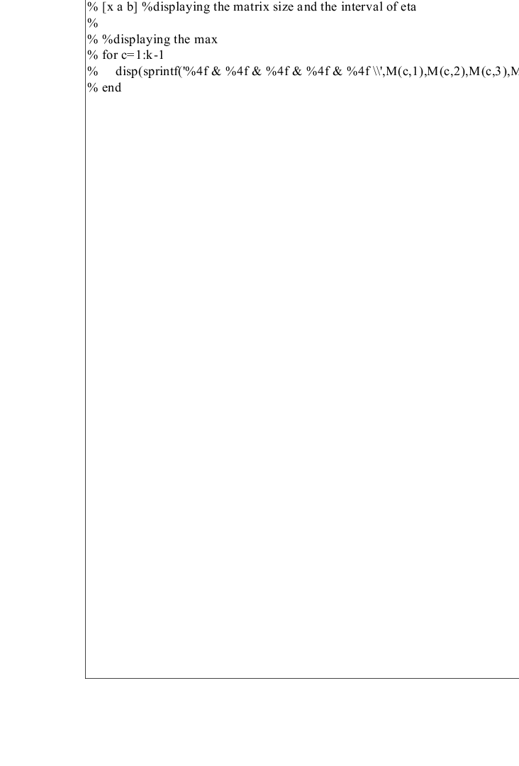
The codes of my three programs: ”spectrum.m”, ”mainresults.m”, and ”decreasingrates.m” are presented below. ”spectrum.m” is in the first box, ”mainresutls.m” is in the second box and third box, and ”decreasingrates.m” is in the fourth box. The percentage signs appeared in the codes represent comment for descriptions and not functioning for certain tasks because ”spectgrum.m” plots versus and separately and ”mainresults.m” graphs , , and calculates the maxima of the square normalized components of those eigenvectors at different time as well.
References
- [MN] Tom Michoel, Bruno Nachtergaele The Large-Spin Asymptotics of the Ferromagnetic XXZ Chain. arXiv:math-ph/0307051 v1 24 Jul 2003 (to appear in Markov Processes and Related Fields).
- [HN] John K. Hunter, Bruno Nachtergaele Applied Analysis. World Scientific. (2001).
- [D] E. B. Davies Spectral Theory and Differential Operators. Cambridge University Press (1996)
- [L] Peter D. Lax Functional Analysis. Wiley (2002)
- [E] Lawrence C. Evans Partial Differential Equations. American Mathematical Society (1998)
- [K] Tosio Kato Perturbation Theory for Linear Operators. (1980)