Homotopy and cohomology of spaces
of locally convex curves in the sphere

A curve $\gamma:[0,1]\to{\mathbb{S}}^{2}$ is called locally convex if its geodesic curvature is always positive, i.e., if $\det(\gamma(t),\gamma^{\prime}(t),\gamma^{\prime\prime}(t))>0$ for all $t$. Let $X$ be the space of all locally convex curves with prescribed initial point and initial direction: $\gamma(0)=e_{1}$ and $\gamma^{\prime}(0)=c_{0}e_{2}$ for some $c_{0}>0$. We define $X_{Q}\subset X$ to be the spaces of curves with prescribed final point and final direction. More precisely, for $Q\in SO(3)$, $X_{Q}$ is the set of $\gamma\in X$ for which $\gamma(1)=Qe_{1}$ and $\gamma^{\prime}(1)=c_{1}Qe_{2}$ for some $c_{1}>0$. In particular, $X_{I}$ is the set of closed parametrized curves of positive geodesic curvature with a prescribed base point and base direction. The topology in these spaces of curves can be taken to be $C^{\infty}$, $C^{k}$ for some $k\geq 2$ or $H^{k}$ (as in Sobolev spaces) for some $k\geq 2$: it actually makes very little difference since it is easy to smoothen out a curve while keeping its geodesic curvature positive. In this paper we discuss the homotopy type and cohomology of the spaces $X_{Q}$. The topology of these spaces has been discussed, among others, by Little ([7]), B. Shapiro, M. Shapiro and Khesin ([9], [10], [8]) but, as far as we could ascertain, the main results presented here are new.

Let $Y_{Q}$ be the set of parametrized curves $\gamma:[0,1]\to{\mathbb{S}}^{2}$ with $\gamma^{\prime}(t)\neq 0$ for all $t$, $\gamma(0)=e_{1}$, $\gamma^{\prime}(0)=c_{0}e_{2}$, $\gamma(1)=Qe_{1}$, $\gamma^{\prime}(1)=c_{1}Qe_{2}$ ($c_{0},c_{1}>0$). Clearly $X_{Q}\subset Y_{Q}$. For each $\gamma\in Y_{Q}$, define $\Gamma:[0,1]\to SO(3)$ by

$R(t)$ being an upper triangular matrix with positive diagonal (the left hand side is the $3\times 3$ matrix with columns $\gamma(t)$, $\gamma^{\prime}(t)$ and $\gamma^{\prime\prime}(t)$). In other words,

Recall that the universal (double) cover of $SO(3)$ is ${\mathbb{S}}^{3}\subset{\mathbb{H}}$, the group of quaternions of absolute value $1$: define $\tilde{\Gamma}:[0,1]\to{\mathbb{S}}^{3}$ by $\tilde{\Gamma}(0)=1$, $\Pi\circ\tilde{\Gamma}=\Gamma$ where $\Pi:{\mathbb{S}}^{3}\to SO(3)$ is the canonical projection. This defines an injective map from $Y_{Q}$ to $Z_{z}\cup Z_{-z}$, where $z$ is a quaternion with $|z|=1$, $\Pi(z)=Q$ and $Z_{z}$ is the set of continuous maps $\alpha:[0,1]\to{\mathbb{S}}^{3}$ with $\alpha(0)=1$ and $\alpha(1)=z$. Clearly each $Z_{z}$ is homotopically equivalent to $Z_{1}=\Omega{\mathbb{S}}^{3}$, the space of continuous maps $\alpha:[0,1]\to{\mathbb{S}}^{3}$ with $\alpha(0)=\alpha(1)=1$. From the Hirsch-Smale theorem ([11], [6]), the map $Y_{Q}\hookrightarrow Z_{z}\cup Z_{-z}$ is a homotopy equivalence. In particular, $Y_{Q}$ has two connected components, each one mapped to one of $Z_{z}$ and $Z_{-z}$: call them $Y_{z}$ and $Y_{-z}$.

Theorem 1 implies that $X_{Q}$ has at least two connected components, one in each of $Y_{\pm z}$. Actually, we shall describe a set $A\subset{\mathbb{S}}^{3}$ with the following propoerties. If $z\not\in A$, then $X\cap Y_{z}$ is connected: we call this set $X_{z}$. If $z\in A$, then $X\cap Y_{z}$ has two connected components $X_{z}$ and $X_{z,c}$: the inclusion $X_{z}\subset Y_{z}$ is homotopically surjective and $X_{z,c}$ is contractible. These facts will be proved in theorems 6 and 7. Since $A$ and $-A=\{-z,z\in A\}$ will turn out to be disjoint, $X_{Q}$ may have two or three components, depending on $Q$. In [7], Little proved that $X_{I}$ has three connected components. B. Shapiro, M. Shapiro and Khesin studied the connected components of other $X_{Q}$ and studied a similar problem in higher dimensions ([8], [9], [10]).

We know that $H^{\ast}(Y_{z},{\mathbb{R}})=H^{\ast}(\Omega{\mathbb{S}}^{3},{\mathbb{R}})={\mathbb{R}}[{\bf x}]$ where ${\bf x}\in H^{2}(\Omega{\mathbb{S}}^{3},{\mathbb{R}})$. Theorem 1 implies that the map $H^{\ast}(i_{z}):H^{\ast}(Y_{z},{\mathbb{R}})\to H^{\ast}(X_{z},{\mathbb{R}})$ is injective and therefore $\dim H^{n}(X_{z},{\mathbb{R}})>0$ for all even $n$. In particular, $X_{z}$ is not homotopically equivalent to a finite CW-complex.

The two spaces $X_{1}$ and $X_{-1}$ are the objects of central interest in this paper. We just saw that their homotopy and cohomology is at least as large as that of $\Omega{\mathbb{S}}^{3}$, and we shall see that the inclusion $X_{z}\subset Y_{z}$ is not a homotopy equivalence in either case. On the other hand, the maps $\pi_{n}(i_{z}):\pi_{n}(X_{z})\to\pi_{n}(Y_{z})$ are isomorphisms for $n\leq 1$.

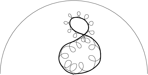
The maps $\pi_{n}(i_{z}):\pi_{n}(X_{z})\to\pi_{n}(Y_{z})$ and, more generally, $[K,i_{z}]:[K,X_{z}]\to[K,Y_{z}]$ are surjective. The choice of the map $g$ in theorem 1 is uniform up to homotopy: intuitively, $g$ is obtained from $f$ adding many small positively oriented loops along each $\gamma=f(k)$ so that the geodesic curvature of $\gamma$ becomes positive (see figure 6). This defines maps $w_{z,K}:[K,Y_{z}]\to[K,X_{z}]$ such that $[K,i_{z}]\circ w_{z,K}$ is the identity. In particular we have injective maps $w_{z,{\mathbb{S}}^{n}}:\pi_{n}(Y_{z})\to\pi_{n}(X_{z})$ which allow us to identify $\pi_{n}(Y_{z})$ with a subgroup of $\pi_{n}(X_{z})$. Let $G_{n,z}$ be the kernel of $\pi_{n}(i_{z})$: we have a natural isomorphism between $\pi_{n}(X_{z})$ and $\pi_{n}(Y_{z})\oplus G_{n,z}$.

For $\gamma_{1}\in Y_{I}$ and $\gamma_{2}\in Y_{Q}$, set $(\gamma_{1}\ast\gamma_{2})(t)=\gamma_{1}(2t)$ for $t\leq 1/2$ and $(\gamma_{1}\ast\gamma_{2})(t)=\gamma_{2}(2t-1)$ for $t\geq 1/2$, thus defining $\ast:Y_{I}\times Y_{Q}\to Y_{Q}$. For $k>0$, let $\nu^{k}\in X_{I}$ be given by

Define $p^{k}_{Q}:X_{Q}\to X_{Q}$ by $p^{k}_{Q}(\gamma)=\nu^{k}\ast\gamma$. It turns out that $p_{Q}=p^{1}_{Q}$ takes $X_{z}$ to $X_{-z}$ and vice versa.

Let $p^{k}_{z}$ be the restriction of $p^{k}_{Q}$ to $X_{z}\subset X_{Q}$. It follows from theorem 3 that the map $\pi_{n}(p^{2}_{z}):\pi_{n}(X_{z})\to\pi_{n}(X_{z})$ is a projection and that the kernel of $\pi_{n}(p^{2}_{z})$ is $G_{n,z}$. We do not know what the groups $G_{n,z}$ are: we know, however, that they are nontrivial.

We can also say something about the cohomology of $X_{z}$.

This work was motivated by the study of the differential equation of order 3:

The set of pairs of potentials $(h_{0},h_{1})$ for which equation $(\dagger)$ admits 3 linearly independent periodic solutions is homotopically equivalent to $X_{I}$. This appears to be the same motivation as that of B. Shapiro and M. Shapiro for studying these same spaces. This topological study of differential equations is continuation of the work done together with Dan Burghelea and Carlos Tomei in [4] and [5].

The author would like to thank Dan Burghelea for helpful conversations. The author acknowledges the hospitality of The Mathematics Department of The Ohio State University during the winter quarter of 2004 and the support of CNPq, Capes and Faperj (Brazil).

The results in this section are not new are are presented to fix notation and for the convenience of the reader; see [1] for more information concerning the geometry of curves in the sphere.

Recall that the unit tangent bundle of ${\mathbb{S}}^{2}$ is $SO(3)$: indeed, the base point, the unit tangent vector and the cross product of the two are the columns of an orthogonal matrix. Also, $\pi_{1}(SO(3))={\mathbb{Z}}/(2)$ and the universal (double) cover of $SO(3)$ is ${\mathbb{S}}^{3}\subset{\mathbb{H}}$, the group of quaternions of absolute value equal to 1. We fix notation by taking the projection $\Pi:{\mathbb{S}}^{3}\to SO(3)$ to be given by

For an immersion $\gamma:[0,1]\to{\mathbb{S}}^{2}$, define $\Gamma:[0,1]\to SO(3)$ by

$R(t)$ being an upper triangular matrix with positive diagonal (the left hand side is the $3\times 3$ matrix with columns $\gamma(t)$, $\gamma^{\prime}(t)$ and $\gamma^{\prime\prime}(t)$). In other words,

If $\gamma(0)=e_{1}$ and $\gamma^{\prime}(0)=ce_{2}$, $c>0$, define $\tilde{\Gamma}:[0,1]\to{\mathbb{S}}^{3}$ by $\tilde{\Gamma}(0)=1$, $\Pi\circ\tilde{\Gamma}=\Gamma$.

For instance, if $\theta\in(0,\pi)$, set

The curve $\gamma$ is a circle in a plane passing through $e_{1}$, parallel to $e_{2}$ and making an angle $\theta$ with $e_{3}$. Notice that $\nu$, as defined in the introduction, is $\nu_{\pi/4}$, that $\nu_{\theta}\in X_{I}$ for $\theta<\pi/2$ and that $\nu_{\pi/2}$ is a geodesic. A simple computation yields

and $\tilde{\Gamma}(t)=\exp(\pi\ell t)$ where $\ell=\cos(2\theta)i+\sin(2\theta)k$. In particular, $\tilde{\Gamma}(1)=-1$ for all $\theta$.

The map $\phi$ taking $\gamma$ to $\Gamma$ defines a map from $Y_{Q}$ to $Z_{Q}$, the set of maps $f:[0,1]\to SO(3)$ with $f(0)=I$ and $f(1)=Q$. Notice that $Z_{Q}$ is naturally identified with $Z_{z}\cup Z_{-z}$ where $z$ and $-z$ are the two preimages of $Q$ under $\Pi$ and $Z_{z}$ is the set of maps $f:[0,1]\to{\mathbb{S}}^{3}$ with $f(0)=1$ and $f(1)=z$. Clearly, $Z_{Q}$ is homotopically equivalent to $\Omega SO(3)=Z_{I}$ and each $Z_{z}$ is homotopically equivalent to $\Omega{\mathbb{S}}^{3}=Z_{1}$.

Recall that $\pi_{n}(\Omega{\mathbb{S}}^{3})=\pi_{n+1}({\mathbb{S}}^{3})$: this implies that each $Z_{z}$ is connected and simply connected with $\pi_{2}(Z_{z})={\mathbb{Z}}$. Also, $H^{\ast}(Z_{z},{\mathbb{R}})=H^{\ast}(\Omega{\mathbb{S}}^{3},{\mathbb{R}})={\mathbb{R}}[{\bf x}]$ where ${\bf x}\in H^{2}(\Omega{\mathbb{S}}^{3},{\mathbb{R}})$ satisfies ${\bf x}^{n}\neq 0$ for all $n$ (see, for instance, [2]).

The Hirsch-Smale theorem proves that $\phi:Y_{Q}\to Z_{Q}$ is a homotopy equivalence: this fact admits a direct, simple proof in our special case but we do not discuss it. As a consequence, each $Y_{z}$ is connected and simply connected, $\pi_{2}(Y_{z})={\mathbb{Z}}$ and $H^{\ast}(Y_{z},{\mathbb{R}})={\mathbb{R}}[{\bf x}]$.

As in the introduction, define $p^{k}_{Q}:Y_{Q}\to Y_{Q}$ by $p^{k}_{Q}(\gamma)=\nu^{k}\ast\gamma$. Notice that $p^{k}_{Q}$ as defined here is trivially homotopic to the composition of $k$ copies of $p_{Q}=p^{1}_{Q}$, justifying the notation. The fact that $\nu\in Y_{-1}$ implies that $p_{Q}:Y_{Q}\to Y_{Q}$ takes $Y_{z}$ to $Y_{-z}$ and vice-versa.

Figure 1 shows how to move from that to a reparametrization of $\gamma$ where a time slightly longer than $1/2$ is spent in a short initial segment. The figure shows only the beginning of $\gamma$: we do not think a formula is necessary or helpful.     $\blacksquare$

Given a parametrized curve of positive geodesic curvature $\gamma:[0,1]\to{\mathbb{S}}^{2}$, let $V_{\gamma}\subseteq{\mathbb{R}}^{3}$ be the closure of the set of all positive linear combinations $a_{1}\gamma(t_{1})+\cdots+a_{n}\gamma(t_{n})$, where $a_{1},\ldots,a_{n}$ are positive real numbers and $t_{1},\ldots,t_{n}\in[0,1]$. The set $V_{\gamma}$ is either a closed convex cone or ${\mathbb{R}}^{3}$. We say that $\gamma$ is convex if $\gamma$ is simple and the image of $\gamma$ is contained in the boundary of $V_{\gamma}$.

Let $X_{Q,c}\subset X_{Q}$ be the set of convex curves $\gamma:[0,1]\to{\mathbb{S}}^{2}$ with $\gamma(0)=e_{1}$, $\gamma^{\prime}(0)=c_{0}e_{2}$, $\gamma(1)=Qe_{1}$ and $\gamma^{\prime}(1)=c_{1}Qe_{2}$ ($c_{0},c_{1}>0$). For $z$ with $\Pi(z)=Q$, define $X_{z}=(X_{Q}-X_{Q,c})\cap Y_{z}$: we shall prove in theorem 7 that each $X_{z}$ is connected. For $Q=I$, this is proved in [7]. In particular, $\nu\in X_{I,c}$, $\nu^{2n}\in X_{1}$ and $\nu^{2n+1}\in X_{-1}$ for $n$ a positive integer.

We show how to decide, given $Q$, whether $X_{Q,c}$ is empty or not. The criterion is harder to state than to prove, so instead of proclaiming a proposition we explain the criterion together with its justification. We split our discussion into three cases: $Qe_{1}=e_{1}$, $Qe_{1}=-e_{1}$ and $Qe_{1}$ and $e_{1}$ linearly independent.

If $Qe_{1}=e_{1}$, let $\alpha\in(-\pi,\pi]$ be the angle from $Qe_{2}$ to $e_{2}$. If $\alpha<0$ then $X_{Q,c}=\emptyset$: the points $\gamma(t)$ fot $t$ near $0$ or $1$ cannot possibly be in the boundary of $V_{\gamma}$ if $\gamma\in X_{Q}$ (see figure 2, (a): the region within the dashed line must belong to $V_{\gamma}$). Similarly, if $\alpha=\pi$ (see figure 2, (b)). On the other hand, if $0\leq\alpha<\pi$, it is easy to construct $\gamma\in X_{Q,c}$ (see figure 2. (c)).

If $Qe_{1}=-e_{1}$, we always have $X_{Q,c}=\emptyset$. Indeed, if a convex cone contains both $e_{1}$ and $-e_{1}$, it must be bounded by two half-planes and there is no curve of positive geodesic curvature contained the intersection of these halfplanes with the unit sphere.

Finally, consider the case when $e_{1}$ and $Qe_{1}$ are linearly independent. Draw the shortest geodesic $\delta$ from $e_{1}$ to $Qe_{1}$: notice that $\delta$ is contained in $V_{\gamma}$ for any $\gamma\in X_{Q}$. Let $v_{0}$ and $v_{1}$ be the tangent vectors to $\delta$ at $e_{1}$ and $Qe_{1}$ (see figure 3). Let $\alpha_{0}$ (resp. $\alpha_{1}$) be the angle from $e_{2}$ to $v_{0}$ (resp. from $v_{1}$ to $Qe_{2}$), $\alpha_{i}\in(-\pi,\pi]$. If $\alpha_{0}\leq 0$ or $\alpha_{1}\leq 0$ then $X_{Q,c}=\emptyset$ (see figure 3, (b): the region within the dashed line must belong to $V_{\gamma}$). On the other hand, if $\alpha_{0}>0$ and $\alpha_{1}>0$ then it is easy to construct $\gamma\in X_{Q,c}$: just keep close to $\delta$ (see figure 3, (c)).

Let $A\subset{\mathbb{S}}^{3}$ be the set of quaternions $z$ for which there exists a convex curve in $Y_{z}$. The paragraphs above give a description of $A$. The set $A$ is neither closed nor open and its interior is given by

The sets $A$ and $-A$ are disjoint, but their closures are not.

From the discussion above, in all cases there exists $v\in{\mathbb{S}}^{2}$, $v\perp e_{1}$, $v\perp Qe_{1}$ such that $\langle v,\gamma(t)\rangle>0$ for all $\gamma\in X_{Q,c}$, $t\in(0,1)$. Indeed, if $Qe_{1}=e_{1}$ we may take $v=e_{3}$ and if $Qe_{1}\neq e_{1}$ we take $v$ to be one of the vectors perpendicular to the geodesic $\delta$.

Let $p$ be the plane $\{u|\langle v,u\rangle=1\}$. For each $\gamma\in X_{Q,c}$, use radial projection to define a curve $\hat{\gamma}:(0,1)\to p$ such that $\hat{\gamma}(t)$ is a positive multiple of $\gamma(t)$. This defines a bijection from $X_{Q,c}$ to the set of curves of positive curvature in the plane with prescribed asymptotic behavior when $t$ tends to $0$ or $1$ ($\gamma(0)$ and $\gamma(1)$ indicate the asymptotic direction and $\gamma^{\prime}(0)$ and $\gamma^{\prime}(1)$ indicate the asymptotic line or lack thereof). By putting axes in an appropriate position, the image of $\hat{\gamma}$ is the graph of a convex function from ${\mathbb{R}}$ to ${\mathbb{R}}$ (with prescribed asymptotic behavior). The parametrization of the curve does not affect the homotopy type of the space of curves, and we therefore have a homotopy equivalence between $X_{Q,c}$ and a convex space: this proves its contractibility.     $\blacksquare$

We now give an explicit generator for $\pi_{2}(Y_{1})$. This function actually has the from $f_{1}:{\mathbb{S}}^{2}\to X_{I}\subset Y_{I}$ and will play an important part throughout the paper. Let

The curve $g_{0}$ is a circle drawn $4$ times and the curve $g_{\pi}$ is a circle drawn $2$ times. A computation verifies that $\det(g_{s}(t),g^{\prime}_{s}(t),g^{\prime\prime}_{s}(t))>0$ for all $s$ and $t$. Let $\Gamma_{s}(t)$ be defined as above. It easy to verify that

for all $s$ and $t$. Finally, let $f_{1}:[0,2\pi]\times[0,\pi]\to X_{I}$ be defined by

If $s_{2}=0$ or $\pi$, the value of $s_{1}$ is irrelevant for the value of $f_{1}$: actually, $f_{1}(s_{1},0)=\nu^{4}$ and $f_{1}(s_{1},\pi)=\nu^{2}$. Also, the remark above shows that $f_{1}(0,s_{2})=f_{1}(2\pi,s_{2})$ for all $s_{2}$. Performing these identifications, the domain of $f_{1}$ becomes the sphere ${\mathbb{S}}^{2}$.

If we follow the identification of $\pi_{2}(Y_{I})$ with $\pi_{3}(SO(3))$ described in the previous section, we see that in order to verify that $f_{1}$ is indeed a generator of $\pi_{2}(Y_{I,+})$ we have to compute the topological degree of the function $\tilde{f}_{1}:{\mathbb{S}}^{2}\times{\mathbb{S}}^{1}\to{\mathbb{S}}^{3}$ which is the double cover of $\hat{f}_{1}:{\mathbb{S}}^{2}\times{\mathbb{S}}^{1}\to SO(3)$ given by

the absolute value of the degree of $\tilde{f}_{1}$ is $1$, confirming that it is a generator. In order to see that, it suffices to verify that $j\in{\mathbb{S}}^{3}$ is a regular value with a single preimage under $\tilde{f}_{1}$; we skip the details.

Figure 4 should give a rough idea of the image of a line $(s_{1},\cdot)$ under $f_{1}$. The fat dot in the figure is $e_{1}$; between the second and third images most of the curve went around the sphere. Figure 5 shows the image of a line $(\cdot,s_{2})$: the first and last curves are intentionally equal: this is a closed curve in $X_{I}$.

More generally, we construct, for each $z\in-A$, a function $f_{z}:{\mathbb{S}}^{2}\to X_{z}$ which is a generator of $\pi_{2}(Y_{z})$. Here, instead of a formula, we indicate the construction in figure 19. The dashed line is an arbitrary curve $\delta:[0,1]\to{\mathbb{S}}^{2}$ with $\delta(0)=Qe_{1}$ ($\Pi z=Q$) and $\delta(1)=e_{1}$ such that $\gamma\ast\delta$ is convex for $\gamma\in X_{-z,c}$. The top and bottom lines are adjacent, forming a cylinder. The curves shown are all contained in a relatively small portion of the sphere and in the transition from the third to the fourth column, most of the curve passed around the back of the sphere. The way to define $f_{z}$ in each of the 24 squares in this grid should be visually obvious (perhaps with a little effort). The octagons on the right and left can likewise be filled in a natural way, having in mind that the center of each octagon is approximately a circle drawn two or four times. The function $f_{1}$ constructed above is a special case of $f_{z}$.

Finally, for a positive integer $n$ and $z=(-1)^{n}z^{\prime}$, $z^{\prime}\in A$, let $\gamma_{0}\in X_{z^{\prime},c}$ be fixed but arbitrary, $\tilde{\Gamma}_{0}:[0,1]\to{\mathbb{S}}^{3}\subset{\mathbb{H}}$ be the associated function. For $i=1,2,\ldots,n$ set $z^{\prime}_{i}=(\tilde{\Gamma}_{0}((i-1)/n))^{-1}\tilde{\Gamma}_{0}(i/n)$ and $z_{i}=-z^{\prime}_{i}$ so that $z^{\prime}=z^{\prime}_{1}z^{\prime}_{2}\cdots z^{\prime}_{n}$ and $z=z_{1}z_{2}\cdots z_{n}$. Notice that $z^{\prime}_{i}\in A$. Set $Q_{i}=\Pi(z_{i})=\Pi(z^{\prime}_{i})$ and define $f^{[n]}_{z}:({\mathbb{S}}^{2})^{n}\to X_{z}$ by

Here we are stretching a bit our original definition of $\ast$: if $\gamma_{1},\gamma_{2}:[0,1]\to{\mathbb{S}}^{2}$ satisfy $\gamma_{1}(1)=\gamma_{2}(0)$ then

Also, for $\gamma\in X$ and $Q\in SO(3)$, $Q\gamma$ is the function from $[0,1]$ to ${\mathbb{S}}^{2}$ defined by $(Q\gamma)(t)=Q(\gamma(t))$.

The following lemma is a simple consequence of the existence of $f_{1}$.

Our function $f_{1}$ shows that $\nu^{2}$ and $\nu^{4}$ are in the same connected component; it follows from that that, for any $n>0$, $\nu^{2+n}\sim\nu^{n}\ast\nu^{2}$ and $\nu^{4+n}\sim\nu^{n}\ast\nu^{4}$ are also in the same connected component. The value of $\theta$ can be changed continuously and is therefore not a problem. The result follows.     $\blacksquare$

Recall that it follows from the results of the previous section that $\nu\in X_{-1,c}$ is not in the same connected component of $X_{I}$ as $\nu^{3}\in X_{-1}$.

For $\gamma\in Y_{Q}$ and corresponding $\Gamma:[0,1]\to SO(3)$, define $F_{n,\theta}(\gamma)(t)=\Gamma(t)\nu_{\theta}^{2n}(t)$. Intuitively, for small values of $\theta$, $F_{n,\theta}(\gamma)$ is obtained from $\gamma$ by attaching $2n$ positively oriented small loops along $\gamma$ (see figure 6).

References

- [1] Arnol’d, V. I., The geometry of spherical curves and the algebra of quaternions, Russian Math. Surveys 50:1, 1-68, 1995.
- [2] Bott, R. and Tu, L., Differential forms in algebraic topology, Spinger-Verlag, GTM 82, New York, 1982.
- [3] Burde, G. and Zieschang, H., Knots, Walter de Gruyter, Berlin, 1985.
- [4] Burghelea, D., Saldanha, N. and Tomei, C., Results on infinite dimensional topology and applications to the structure of the critical set of non-linear Sturm-Liouville operators, J. Differential Equations, 188, 569-590, 2003.
- [5] Burghelea, D., Saldanha, N. and Tomei, C., The topology of the monodromy map of the second order ODE and the structure of the critical set of nonlinear Sturm-Liouville operators, preprint.
- [6] Hirsch, M., Immersions of manifolds, Trans. Am. Math. Soc. 93, 242-276, 1959.
- [7] Little, J. A., Nondegenerate homotopies of curves on the unit 2-sphere, J. Differential Geometry, 4, 339-348, 1970.
- [8] Shapiro, B. and Khesin, B., Homotopy classification of nondegenerate quasiperiodic curves on the -sphere, Publ. Inst. Math. (Beograd) 66(80), 127-156, 1999.
- [9] Shapiro, B. and Shapiro, M., On the number of connected components of nondegenerate curves on , Bull. of the AMS, 25, 75-79, 1991.
- [10] Shapiro, M., Topology of the space of nondegenerate curves, Math. USSR, 57, 106-126, 1993.
- [11] Smale, S., The classification of immersions of spheres in euclidean spaces, Ann. of Math. 69, 327-344, 1959.
Nicolau C. Saldanha, PUC-Rio
nicolau@mat.puc-rio.br; http://www.mat.puc-rio.br/nicolau/
Departamento de Matemática, PUC-Rio
R. Marquês de S. Vicente 225, Rio de Janeiro, RJ 22453-900, Brazil