Contact homology and one parameter familiesof Legendrian knots
Abstract
We consider –families of Legendrian knots in the standard contact . We define the monodromy of such a loop, which is an automorphism of the Chekanov–Eliashberg contact homology of the starting (and ending) point. We prove this monodromy is a homotopy invariant of the loop (Theorem 1.1). We also establish techniques to address the issue of Reidemeister moves of Lagrangian projections of Legendrian links. As an application, we exhibit a loop of right-handed Legendrian torus knots which is non-contractible in the space of Legendrian knots, although it is contractible in the space of smooth knots. For this result, we also compute the contact homology of what we call the Legendrian closure of a positive braid (Definition 6.1) and construct an augmentation for each such link diagram.
keywords
Legendrian contact homology, monodromy, Reidemeister moves, braid positive knots, torus knots53D40 \secondaryclass57M25
eometry & opology
![[Uncaptioned image]](0407347v2/gtlogo.png) Volume 9 (2005)
2013–2078\nlPublished: 26 October 2005
Volume 9 (2005)
2013–2078\nlPublished: 26 October 2005
Email:\stdspace\theemail
URL:\stdspace\theurl
Abstract
AMS Classification numbers Primary: \theprimaryclass
Secondary: \thesecondaryclass
Keywords: \thekeywords
Proposed: Yasha Eliashberg Received: 3 October 2004\nlSeconded: Peter Ozsváth, Tomasz Mrowka Revised: 24 July 2005
1 Introduction
A Legendrian knot is an embedding which is everywhere tangent to the kernel of the standard contact –form . Two such knots are equivalent if they are homotopic through Legendrian knots. This is a refinement of the obvious subdivision according to classical knot type; just how much finer is a topic of current research. (We may refer to this as the –problem of the space of Legendrian knots). The integer-valued invariants (Thurston–Bennequin number) and (rotation number) guarantee that every classical knot type contains infinitely many Legendrian equivalence classes. It was a major break-through when Chekanov [6] introduced a much more complicated, Floer-theoretical invariant which was able to distinguish between Legendrian knots of the same , , and classical type (since then, Etnyre and Honda [11, 12, 13] have been able to prove similar results with different methods). The form in which we’ll consider Chekanov’s invariant is that of a system of homology groups, which we will call contact homology.
In this paper we use contact homology to tackle another, so called –problem; namely, we use monodromy induced on this homology to provide the first examples that Legendrian and classical knots are different at the level of –parameter families.
1.1 Statements of results
In its most general formulation, Chekanov’s invariant of Legendrian knots [6] takes the form of a stable tame isomorphism class of differential graded algebras, or DGA’s for short, . What’s more important for us is that in particular, the homology is an invariant of the Legendrian knot type. This homology, which is actually also a graded algebra over , will be referred to as contact homology and will be denoted by , where is a (representative of a) Legendrian knot type. In [14], Etnyre, Ng, and Sabloff defined a natural extension of Chekanov’s work, namely a DGA and corresponding contact homology with –coefficients. We will carry out our proofs in this more general setting, even though in all of the applications known to the author the original –version (which will be used in sections 6–10) would be sufficient.
The main result of the paper is the following:
Theorem 1.1.
For every Legendrian knot type and generic , there exists a multiplicative homomorphism
defined by continuation on the Chekanov–Eliashberg contact homology . This is true with either or –coefficients.
In particular, monodromy calculations are carried out in the homology and neither in its linearized [6] or abelianized [14] versions, nor in the DGA itself. Augmentations (which are the objects also needed to define linearized homology) do however play an important role in proving that is non-trivial. This will be demonstrated by the following example. Let be the space of positive Legendrian torus knots with maximal Thurston–Bennequin number (where are relatively prime). is connected by a result of Etnyre and Honda [11]. Consider the loop of Figure 1 (a more elaborate definition is in section 8). We claim the following:
Theorem 1.2.
is either an element of infinite order or its order is divisible by .

By Theorem 1.1, this follows immediately from the following:
Theorem 1.3.
The restricted monodromy of the loop , where is the index part of the –coefficient contact homology , has order .
In particular, is different from the identity automorphism, and because doesn’t divide , so is . Thus by Theorem 1.1, is non-trivial. On the other hand, if is the space of smooth positive torus knots, then is trivial11 1 In fact, an elementary application of Hatcher’s work [20] shows that if is odd, then is itself contractible in , and if is even, then has order ., because is homotopic to a rotation by radians and . So Theorem 1.2 had to be demonstrated via a specifically “Legendrian” technique, which is the monodromy invariant . We also have
Corollary 1.4.
There exist Legendrian knot types so that for the corresponding smooth knot type , the homomorphism induced by the inclusion is not injective.
It is an open problem whether this homomorphism, for fixed and , is always surjective. It is also worthwhile to compare our results to those of Benham, Lin, and Miller in [2]. They prove that if is the set of knots in with writhe (so that ) then the inclusion is a weak homotopy equivalence. For results about the homotopy type of , see Hatcher [20].
There are two widely used ways to represent Legendrian knots in the standard contact . In Figure 1, we used the front projection. For most of the paper, however, we will use Lagrangian projections, for the simple reason that is naturally defined in terms of those. (Ng [23] gives a definition in terms of fronts.) Lagrangian projections are also more symmetric, but on the other hand less robust than fronts. By this I mean that certain linear constraints need to be satisfied both for the existence of an actual Legendrian lift of the diagram and for doing Reidemeister moves as well. While [6, section 11] contains a thorough description of the former phenomenon, our Theorem 4.1 appears to be the first account in the literature on the latter problem. We formulate a solution in terms of techniques and language of linear programming.
The paper is organized as follows. In section 1.2 we give some motivation and describe related work. We review some basic material in section 2. Section 3 contains the definition of monodromy and the proof of Theorem 1.1. Section 4 concludes the general discussion of one parameter families of Legendrian links by addressing Reidemeister moves.
Then we turn to examples; section 5 contains the simplest non-trivial one known to the author, a loop of Legendrian trefoils. In section 8 we include it in a much more general class of examples. Those loops consist of so called Legendrian closures of positive braids. Section 6 examines their base points; in particular, we compute their DGA. In section 7 we construct an augmentation for that DGA. Finally, we specialize our discussion again to the case when the Legendrian closure is a positive torus knot and use the last two sections to prove Theorem 1.3.
Acknowledgments\quaThis paper is almost identical to the author’s PhD thesis that was submitted in 2004 at the University of California at Berkeley. It is my pleasure to thank the institution, and in particular my advisors, Rob Kirby and Michael Hutchings, for all the generous support that they provided. It was in fact Mike Hutchings who gave me the idea of this project. I would also like to thank Lenny Ng and Josh Sabloff for checking earlier versions of the manuscript, as well as them, Tobias Ekholm, Michael Sullivan and András Szűcs for stimulating conversations. I was supported by NSF grant DMS-0244558 during part of the research.
1.2 Floer theory
Loosely speaking, the idea of Floer theory is to formulate a Morse-type homology theory of certain real-valued smooth functionals on certain infinite-dimensional manifolds. The manifold and the functional are typically associated to an object such as a pair of Lagrangians, a symplectomorphism, a contact structure, a Legendrian submanifold etc. Some special cases of this project have had great success (alas, analytical details are sometimes missing) and we refer to these as “Floer theories.” We should mention at least one case when the analogy with finite-dimensional Morse theory starts breaking down: in symplectic field theory [9], of which contact homology is a special case [14], generators of Floer homology are indeed critical points of an action functional, but flow lines (which are pseudoholomorphic curves in an appropriate sense) starting from a critical point may split and end at a finite collection of critical points (as opposed to just one endpoint). The natural way to include this phenomenon in our algebraic formulation of the theory is to write the multiple endpoints as a product. This is how the chain complex in this case takes the form of a differential graded algebra (DGA).
Besides finding new Floer theories, it is also an important and promising direction of research to generalize more and more features of finite-dimensional Morse theory to these new settings. One such feature can be the so called continuation map. Suppose , is a –parameter family of smooth functions and Riemannian metrics on the finite-dimensional smooth manifold . Suppose that the family is generic. This in particular means that the pairs are Morse–Smale (ie, they have associated Morse homologies ) with finitely many exceptions . Note that we can not speak of homologies . Yet we may define a vector field on by , where is the negative gradient of with respect to , and after observing that , we may count flow lines of to define a chain map from the Morse complex of to that of . The fact that it induces an isomorphism (which we call the continuation map) can be established by a certain construction of chain homotopies [16], similar in flavor to the above22 2 What has just been outlined is what I call the ‘analytic approach.’ Alternatively, one may study the bifurcations that take place at and define ‘combinatorial’ continuation maps , as well as chain homotopies to guarantee that these are isomorphisms. The approach taken in this paper will in fact be a generalization of the latter.. This provides an alternative proof that the isomorphism class of Morse homology depends only on the manifold, thus making Morse theory a self-contained homology theory.
But the usefulness of the continuation map doesn’t stop here. Consider a fibration with smooth manifold fiber , along with a smooth function and a Riemannian metric on . Suppose that for , the pair is Morse–Smale and the family is generic. Then by continuation, we obtain an automorphism (called monodromy) . This is naturally equivalent to the automorphism of the singular homology of induced by the gluing map of the fibration (which is well defined up to homotopy, therefore its action is well defined). In particular, a non-trivial monodromy implies the non-triviality of the fibration.
As already demonstrated by Seidel [26] and Bourgeois [4], the continuation (monodromy) map can prove non-triviality theorems, in a way analogous to the above, about the fundamental group of the space of objects (“object” means a symplectomorphism in [26] and a contact structure in [4]), to which a version of Floer theory is associated33 3 Strictly speaking, Floer homology is associated only to generic objects. Once we have proven that its isomorphism class is invariant within a path-component of the objects, this distinction becomes immaterial, provided that we only wish to use Floer theory to separate such path-components (ie, we do –theory). But the presence of non-generic objects is potentially an issue again when we investigate the topology of the path-components (like their , as in this paper).. To get such conclusions, it is of course a key point to prove that monodromy is invariant under homotopies of the loop of objects. In this paper we obtain such a result about the space of Legendrian knots .
There is also a generalized invariant of families of objects parametrized by an arbitrary finite-dimensional manifold, recently discovered by Hutchings [21]. The value of this is a spectral sequence. [21] contains its description in the case of finite-dimensional Morse theory, where the spectral sequence associated to a generic –tuple (as above, except that is replaced by the arbitrary finite-dimensional manifold ) turns out to be isomorphic to the Leray–Serre spectral sequence of the fibration. A paper [22] detailing the case of the Floer theory of symplectomorphisms, thus generalizing Seidel’s results, is in preparation. In other Floer theories, apart from Bourgeois’s results (where ) and the present paper (where ), the spectral sequence invariant is yet to be either established (see the next paragraph for more on this when ) or exploited.
The motivation behind the group of results concerning one-parameter families is that Floer homology should not just be viewed as an invariant of certain objects, but should also be treated as a twisted coefficient system over the space of those objects; its non-trivial twisting is then capable of detecting the fundamental group of the moduli space. The existence of this twisted coefficient system, modulo an issue of fixing the signs in the continuation maps (see [21] for more), is an immediate consequence of what’s already in the literature for many versions of Floer theory. These are the versions where they prove topological invariance by constructing continuation maps and chain homotopies using the analytic methods introduced in Floer’s seminal paper [16] (as opposed to a study of bifurcations, which also appears in earlier work of Floer). In these cases the existence of a monodromy invariant, which is equivalent to the spectral sequence when , is automatic too.
However, the invariance of contact homology was established in a different way, namely through a certain combinatorial “bifurcation analysis” [6]. Therefore we can use the analytic considerations mentioned so far only as a source of motivation that the monodromy invariant (and the spectral sequence invariant) exists in this context, even though one suspects that once monodromy is defined analytically, it will agree with our combinatorially defined version44 4 It is proven in [14] that Chekanov’s combinatorially defined homology is isomorphic to the relative contact homology whose analytical definition was outlined in [9] and completed in [7]. For proof of invariance, however, the authors use bifurcation analysis in [7].. Following this “hint” then, we streamline Chekanov’s original proof in section 3.1 (without changing its combinatorial nature) to emphasize the role of continuation more, and then in section 3.2, we continue the combinatorial study of bifurcations to provide the chain homotopies needed to prove that monodromy is a well-defined invariant.
2 Preliminaries
Throughout this paper, we work in the standard contact ; we write the –form, whose kernel field is the contact distribution, as . A curve is called a Legendrian knot if it is embedded (in particular, it has an everywhere non-zero tangent) and . The space of such knots, modulo reparametrization, is denoted by . We will refer to connected components of (with respect to the quotient of the topology) as Legendrian knot types55 5 We will use for actual maps and for their equivalence classes modulo reparametrization, while will be used to denote Legendrian knot types.. When talking about classical or smooth knots, we simply mean that the Legendrian assumption is not made. Modulo reparametrization, these form the moduli space , whose connected components are called classical or smooth knot types.
A (Legendrian or classical) link is a finite disjoint union of knots.
2.1 Link projections
The Lagrangian projection is . If is a Legendrian link, it admits an –projection that is an immersion with the additional properties described below in Proposition 2.2. We call and generic if satisfies the usual assumptions for classical link diagrams, ie, it has no singularities other than finitely many transverse self-crossings.
The front projection is . The image of a generic Legendrian link under this is a smooth curve with finitely many semicubical cusp points, no self-tangencies and no vertical tangents. As , at every crossing the strand with smaller slope is the overcrossing one. Generic homotopies are composed of isotopies and a list of Reidemeister moves (see Figure 2). Unlike for Lagrangian projections, these moves can always be carried out without further restrictions. For example, the definition of in Figure 1 (with Reidemeister II moves and Reidemeister II-1 moves) is sound. For the rest of the paper, we won’t need to use fronts, except occasionally for motivation.

Fix an orientation of the Legendrian knot . Let be a simple transverse self-intersection (crossing) in its Lagrangian projection and denote the difference in –coordinate between the two preimages of by . We will refer to the positive number as the height of . Starting at the undercrossing, follow until we reach again, this time on the upper strand. This path is called the capping path of and we denote it by .
We use capping paths to define the grading, or index of a crossing, as follows. Assume that all crossings happen at a right angle. Then the rotation of the tangent to the capping path (with respect to the orientation of the plane) is an odd multiple of . The grading of the crossing is the integer
| (1) |
The rotation number of a Legendrian knot is the Whitney index of its (oriented) Lagrangian projection. Its sign does depend on the choice of orientation. (However the modulo residue of the grading of a crossing does not depend on the orientation. This residue is the value of Chekanov’s original grading.) The Thurston–Bennequin number of a Legendrian knot is the writhe of its Lagrangian projection, ie, the number of crossings with even grading minus the number of those with odd grading66 6 It is easy to verify that coincides with the sign of the crossing in classical knot theory. This fact is assumed in Figure 3, too.. It doesn’t depend on the orientation of the knot. The parities of and are opposite. The list of the three classical invariants of a Legendrian knot is completed by its classical knot type.

The Reeb signs of the four quadrants surrounding a crossing are defined according to the scheme on the left of Figure 3. For the definition of the DGA with coefficients in the next subsection, we will also need the concept of the so called orientation sign. This is for all quadrants surrounding an oddly graded crossing and at evenly graded crossings, the two marked quadrants of Figure 3 have orientation sign , the other two have . The only property of the orientation signs that matters for the purposes of defining a homology theory is the following:
Lemma 2.1.
[14]\quaAround the crossing , the product of the orientation signs of any two opposite quadrants is .
Let be the crossings of a classical link diagram . Let us denote the bounded components of the complement by . Let and be vector spaces with labeled bases and let and be their respective (open) positive cones. Chekanov defined the linear map by the matrix , where is the number of quadrants at that face , counted with Reeb signs.
Proposition 2.2.
Suppose is the Lagrangian projection of a generic Legendrian link . For the areas of , heights of , and incidence coefficients as described above, we have
| (2) |
Proof.
First, it is an elementary fact that any arc has Legendrian lifts in : let and define . Further, any two such lifts differ by a translation in the direction.
For each , consider a piecewise continuously differentiable closed path that traverses the boundary of once counterclockwise. Suppose it meets the crossings in this order (repetition in the list is allowed). Construct a Legendrian lift of . This is not a closed curve; in fact by Stokes’ theorem, . On the other hand, the same can also be constructed by gluing together –translates of pieces of . Inspecting Figure 3, it is easy to see that the total change of along the latter is exactly , where the counting happens with the opposite of the Reeb sign. ∎
We will also need the following observation from [6] later:
Lemma 2.3.
In the situation of Proposition 2.2,
Remark 2.4.
The equations (2) imply the well known fact that a Lagrangian projection bounds zero area. Indeed, at each crossing, the sum of the indices with respect to of either pair of opposite regions (sharing the same Reeb sign) is the same.
Remark 2.5.
By equation (2), the height vector of a generic Lagrangian projection determines the area vector . Moreover, is such that lies in . In addition to for all , this forces homogeneous linear inequalities for . By satisfying the linear constraints we either mean that is such that and , or that the pair is such that (2) holds.
Definition 2.6.
Let be a classical link diagram and consider the open convex cone
We say that is a Lagrangian diagram if is non-empty.
By the previous remark, Lagrangian projections of generic Legendrian links are Lagrangian diagrams. Lagrangian diagrams are the objects represented in our figures; in particular, we do not draw areas of regions to scale. All Lagrangian diagrams can, though, be isotoped (in the smooth sense) to actual Lagrangian projections (or, equivalently, we can use orientation-preserving diffeomorphisms of to take one diagram to another). Moreover, any element of can be realized this way and because is convex, it is easy to see that all Lagrangian projections with the same underlying Lagrangian diagram can be isotoped into each other (this time in the Legendrian sense, ie, keeping the linear constraints intact throughout). In particular, a Lagrangian diagram represents a well-defined Legendrian link.
Example 2.7.
Consider the knot diagram on the left side of Figure 4. We claim that is non-empty, thus is the Lagrangian diagram of a Legendrian knot . The equations (2) take the following form (note the Reeb signs in Figure 4):
It is easy to check that the choice of , , yields the values , , , , and . As these are all positive, our linear constraints can indeed be satisfied.

The claim can be proven in a less direct way, too: the diagram is the result of the resolution [23] of a certain front diagram, analogous to the base point of the loop of Figure 1. See section 6 for more.
The rotation number of this knot (with either orientation, of course) is . The gradings of the crossings (with either orientation, because ) are and . Hence the Thurston–Bennequin number is . Finally, the classical knot type of is the right-handed trefoil knot.
Remark 2.8.
Let and be arbitrary points on the same component of the Legendrian link . Then and divide into two arcs, and . If is another immersed arc with the same endpoints and starting and ending tangent vectors as , and so that bounds zero area, then possesses a Legendrian lift (in general, an immersion) which coincides with over . This diagrammatical method can be used to construct modifications of Legendrian links that only affect a small segment of the link, although possibly quite dramatically. We will use this idea in sections 4, 6, and 8.
2.2 Knot DGA and homology
Definition 2.9.
Let be a commutative ring. A differential graded algebra, or DGA, is a graded associative algebra over with identity , together with a differential . We will also refer to the grading as the index, which is multiplicative and takes values in a cyclic group . We require that be an index , –linear map so that for all and with pure index (consequently, ), and finally that .
A DGA is called semi-free (with generators ) if its underlying algebra is the ring (tensor algebra) of non-commutative polynomials in a finite collection of pure-index elements . We will use the term degree to refer to the degree of polynomials in this situation.
Throughout the paper, we will use the term polynomial to mean non-commutative polynomial.
Let be an oriented, generic Legendrian knot in with Lagrangian projection . Let the crossings of be . We associate a semi-free DGA to as follows.
The graded algebra\quaLet be the non-commutative, associative, unital polynomial algebra over generated by the symbols . Grade each generator using the value defined by (1) and let (this value, ie twice the rotation number, is often called the Maslov number of the knot). Extend the grading to monomials multiplicatively, obtaining a –grading so that we may write . Note that this grading, also called index, is different from the grading given by the degree of the polynomials.
For each positive integer , fix an oriented disc (thus the boundary is also oriented) with points marked on its boundary in the given cyclic order. A continuous map is admissible with respect to (sometimes we’ll say is an admissible disc in ) if it is an immersion away from the marked points, it preserves the orientation of the disc and moreover it takes to so that each marked point is mapped to a crossing in such a way that locally, the image of the disc forms an angle less than . We also require that the quadrant occupied near the crossing (the so called positive corner) has Reeb sign and all other quadrants, at the so called negative corners , have Reeb sign . We’ll also say that the disc turns at its corners , or that it turns at certain quadrants located at those points.
Note that we didn’t require that the orientations of the curves and match. Let us call an admissible immersion compatible with the orientation of (or a compatible disc) if those two orientations either agree at all points of or disagree at all such points. We will need the following lemma in section 6.
Lemma 2.10.
Let be an oriented Lagrangian diagram. An admissible immersion is compatible with the orientation of if and only if its positive corner has odd index and all of its negative corners have even indices.
Proof.
An immersion is compatible if and only if the orientation requirement is satisfied in arbitrarily small neighborhoods of the punctures. Then the statement follows very easily from the observation (also mentioned in footnote 6) that coincides with the sign of the crossing in classical knot theory. Indeed, the middle diagram of Figure 3 shows an oddly graded crossing and we see (comparing with the diagram on the left) that a compatible disc may only turn at its positive quadrants. The diagram on the right shows an evenly graded crossing and a similar examination yields that compatible discs may only turn at its negative quadrants. ∎
The following lemma is a consequence of Proposition 2.2.
Lemma 2.11.
Let be an admissible immersion. Then
In particular, for all .
The differential\quaTo compute for a given crossing , one considers all admissible immersions, modulo reparametrization, with positive corner . A typical one described above contributes the monomial
where are the orientation signs (see Figure 3) of the quadrants occupied by at its corners, and is defined as follows. Take the union of the oriented segments of (the orientation is induced from that of ) with the capping path and the reversed capping paths . This is a cycle whose homology class in is identified with the integer via the chosen orientation of .
is the sum of these contributions over all admissible immersions. We extend to using –linearity and the signed Leibniz rule .
Theorem 2.12 (Chekanov–Etnyre–Ng–Sabloff).
The sum taken when computing for any crossing is finite, hence is well defined. It has index and satisfies .
Definition 2.13.
The semi-free DGA is called the Chekanov–Eliashberg differential graded algebra associated to the generic Legendrian knot . Its homology is the Chekanov–Eliashberg contact homology, or simply contact homology of .
Chekanov’s main theorem is that (and further, a certain equivalence class of , called its stable tame isomorphism class) is unchanged when one passes to another generic Legendrian knot that is homotopic to through Legendrian knots. (In this case we also say that is Legendrian isotopic to .) We will state this result in Theorem 3.2.
Example 2.14.
The trefoil DGA: please refer to Figure 4 and Example 2.7. We choose the orientation as on the right side of the figure. Quadrants with negative orientation sign are marked. Note that and thus for index reasons, . On the other hand,
| (3) |
The admissible discs contributing these terms are , , , and , respectively. Similarly,
| (4) |
with terms contributed by77 7 This way of describing the actual immersions works fine in this case. In general however it is possible that two different admissible discs cover the same regions with the same multiplicities. As to whether we indeed listed all admissible discs, the reader can check that as an exercise or can refer to section 6, where we shall determine all admissible discs in a certain class of Lagrangian diagrams generalizing . , , , , , and , respectively. Note that all admissible immersions in are compatible with the orientation of the diagram. The following observation will be useful later in the proof of Theorem 1.2 for , :
| (5) |
In other words, in the contact homology.
2.3 DGA maps and the product structure
Chain complexes of homology theories are primarily Abelian groups with a differential. The presence of the (non-commutative) product structure in Chekanov–Eliashberg theory is an ‘extra’ feature. In this section we point out how this does not actually complicate matters; namely, how we can concentrate on generators only and then let the algebra take care of itself. For more on general DGA theory, see [15].
Definition 2.15.
Let and be differential graded algebras (over the same commutative ring and graded by the same cyclic group ). A linear map is a chain map if it is index-preserving and intertwines the differentials: for all . If such a is also an algebra homomorphism, then we call it a DGA morphism.
Definition 2.16.
Let and be differential graded algebras (over the same , graded by the same ), and chain maps between them. An index map is called a –derivation of index if for all of pure index and for all , we have
If and , then we simply speak of a derivation of index .
In this paper we consider three types of DGA mappings. They are all –linear, but each has a different relation to the product structure of the DGA. Namely, by definition, the differential itself is a derivation of index . All chain maps that we consider are going to be DGA morphisms (in particular, they fix constants), and all chain homotopies connecting chain maps , will be –derivations of index (from which it follows that they take constants to ). The following two lemmas show that these self-imposed restrictions are very natural and useful.
Lemma 2.17.
Let and be semi-free differential graded algebras over a commutative ring , graded by . If an index algebra homomorphism is such that for all generators of , then the same holds for all elements (ie, is a chain map).
Moreover, any assignment of values to the generators of which satisfies for all can be uniquely extended to an index algebra homomorphism.
Proof.
To complete a trivial induction proof, we need to show that if and are homogeneous elements of that satisfy the desired property, then such is , too:
In the last assertion, the existence of an extension is obvious, since is semi-free with the given generators and is associative. We just need to check that the unique extension is also of index , which is established with the same induction argument based on noting that if and , then . ∎
Lemma 2.18.
Let and be semi-free differential graded algebras over the commutative ring , graded by , and let be DGA morphisms. If is a –derivation of index so that for all generators of , then the same holds for all elements (ie, is a chain homotopy between and ).
Moreover, any assignment of values to the generators of which satisfies for all can be uniquely extended to a –derivation of index .
Proof.
The first part of the proof is a similar, but longer computation as in the previous argument:
In the second part, to show that the extension is unique, we need to establish that , which is due to the following direct computation:
The extension is also index by the already usual induction argument: If and are homogeneous with and , then , where and , so is homogeneous of index . ∎
Table 1 summarizes the relevant algebraic machinery. For all three rows, it is true that if the ‘map’ is defined on the generators so that the ‘index’ requirement is satisfied and then if it is extended to the whole DGA using linearity and the ‘product identity,’ then
- 1.
such an extension is unique, it satisfies the ‘index’ requirement, and
- 2.
if the ‘property’ requirement holds for the generators, then it holds for all elements of the DGA.
\cl
map
property
index
product identity
differential
chain map
chain homotopy
between chain
1
maps ,
3 The monodromy invariant
Let us first outline the contents of the section. Let be a Legendrian knot type. We call an element of generic, as in section 2, if its Lagrangian projection is generic (this is equivalent to saying that the Legendrian knot doesn’t have degenerate Reeb chords). These are the ones to which a graded chain complex , and a corresponding Floer homology are actually associated. Non-generic objects form a codimension discriminant .
Generic homotopies, ie paths in , meet only the codimension (codimension is always meant with respect to ) stratum and diagrammatically, this corresponds to Reidemeister II, II-1, or III moves (see Figure 6). If and are in adjacent chambers of , then following [6] (and [14] for the case of –coefficients), one is able to write down a chain map , corresponding to the Reidemeister move, that induces an isomorphism . (In [6, 14] they use these chain maps to prove that the homology is independent of the actual projection.) Composing these chain maps/isomorphisms, every generic path that connects generic objects and has an induced isomorphism , called the holonomy of the path. Details are found in section 3.1.
Now to prove that the holonomy only depends on the homotopy class (with fixed endpoints) of , one has to consider two kinds of events: paths that are tangent to (this is easy) and paths that meet . To deal with the latter, we take a small generic loop , starting and ending at the generic element , and linking the codimension discriminant once. While it is not necessarily the case that the induced chain map is the identity, we will establish that there is always a chain homotopy connecting and , thereby proving that on the homology level , as desired.
In Figure 5, we represented a hypothetical case when two strands of the discriminant meet transversally. (As it is shown in [1, Figure 6] and as we’ll see in section 3.2, the local description at other points of may be slightly less or more complicated, but the approach is the same.) As we know that all arrows on the ‘top level’ represent isomorphisms, we may choose any two objects, which may even coincide, and direct all arrows from the first to the second. If this choice of directions can be accompanied with a chain homotopy on the ‘middle level,’ and in section 3.2 we prove that this is always the case, then we indeed get that the diagram of holonomies on the ‘top level’ commutes.
In section 3.3 we review our formulas in their simplified, –coefficient versions.

3.1 Chain maps
Generic paths in are isotopies with a finite number of Reidemeister moves. If we work with Lagrangian projections, then there are four different kinds of the latter, depicted in Figure 6. III and III moves are also called triangle moves. Move II is sometimes referred to as a birth and move II-1 as a death (of a pair of crossings).
Let us denote the DGA’s of the diagrams in the upper row of Figure 6 by and in the lower row, by . The crossings not affected by the moves are in an obvious one-to-one correspondence. If is one of these, then the corresponding crossing in will be denoted by .
Before stating Theorem 3.2, let us review Chekanov’s analysis, although in slightly different terms, of the bifurcation that takes place on the right side of Figure 6. The re-phrasing is possible because we shall only be concerned with the homology, and not the stable tame isomorphism class of the DGA, as our invariant. Let the crossings that generate be arranged by height as follows:
Let , where and are the orientation signs from Figure 6 (it is easy to prove that the exponent of is in the term coming from the vanishing bigon) and by Lemma 2.11, . Define
by putting (), (), , and , where and are the other two orientation signs in Figure 6 and is obtained from in the obvious way of putting primes on all the ’s in the expression. Note that these assignments preserve the grading, so by the second statement of Lemma 2.17, we can extend to a well-defined index algebra homomorphism. The geometric content of the bifurcation is captured by the following result of Chekanov:
Lemma 3.1.
is a chain map.
One of the statements of Theorem 3.2 is that induces an isomorphism of homologies. Our goal now is to define what will be its homotopy inverse, that is another chain map88 8 All of the considerations leading up from this point to Theorem 3.2 are purely algebraic. The chain map is less explicit in [6] and [14] than in what follows. . While it will be the case that , and will only be chain homotopic via a certain . In fact, we will build and with a somewhat subtle simultaneous construction99 9 In Remark 3.4, we express in even more explicit terms and without referring to . That description is needed for applications, but would be impractical in the theoretical discussion., using the filtration that we will introduce next.
Define
for all . Note that by Lemma 2.11, and . It follows that and are DGA’s themselves1010 10 It is not true though that, for example, would map to ; is usually not in . for all . Furthermore, for all such , the restriction
is a DGA morphism. Define the index algebra homomorphism
by (). By Lemma 2.17, this is also a chain map, for . Here we used Lemma 3.1 and that by Lemma 2.11, can’t contain or , and finally, the obvious fact that .
Now, and are both DGA endomorphisms of . By the second statement of Lemma 2.18, the last three rows of the assignment
| (6) |
can be uniquely extended to a –derivation
of index ; note that indeed, because is of index , we have . Then we use the first part of Lemma 2.18 to show that is a chain homotopy between and : For the generators , the condition holds by the observation at the end of the previous paragraph, together with the fact, following from the definition, that the restriction of to the DGA is . For and , it is established below:
by Lemma 2.1, and
On the other hand,
Next, we use a recursive process to define extensions of and to the whole of and , respectively. Suppose that for some value , the DGA morphism and the –derivation of index are already defined so that is a chain homotopy between and . Extend to by letting
| (7) |
As this preserves the grading of , by Lemma 2.17 (second part) there does exist an extension, which is an index algebra homomorphism . To see that it’s also a DGA morphism, we use Lemma 2.17 (first part), the inductive hypothesis, and the following computation:
which works because and .
Now we are in a position to use the DGA morphisms and , along with the relevant values from (6) to define the –derivation of index , which is obviously an extension of the previous . To make sure that is also a chain homotopy between and , we still have to check that for , but it’s a tautology: .

Theorem 3.2 (Chekanov).
The following maps, when extended to as algebra homomorphisms, are chain maps that induce isomorphisms (as graded algebras) of the corresponding Chekanov–Eliashberg contact homologies. (Recall that is the DGA of the upper row, and is the DGA of the lower row in Figure 6.)
- 1.
Move III: Let , , , and , where is any generator of not shown in Figure 6.
- 2.
Move III: Let
where , , and are the orientation signs of the quadrants indicated in Figure 6 and is the winding, with respect to the chosen orientation of the knot, of the union of capping paths (thought of as starting and ending at the single point that the triangle shrinks to). Other generators are mapped trivially: , , and .
- 3.
Move II-1: Let (recall that does not contain neither nor ). Define , which gives rise to the obvious re-labeling . Then let
(this is the map of the preceding discussion).
- 4.
Move II: The map , constructed in the preceding paragraphs (for a more explicit description, see Remark 3.4).
Proof.
We cite [6] and [14] that the maps associated to III, III, and II-1 moves are indeed chain maps (cf Lemma 3.1), and we have already seen that is one. In each of the four cases, the reverse of the move is again a Reidemeister move, with a corresponding chain map associated to it. It is enough to prove that the relevant pairwise compositions of these chain maps are chain homotopic to the identity. This is obvious for the pair of III moves on the left side of Figure 6. For the pair of III moves in the middle, note that the reverse move sends
where , , and are the orientation signs of the quadrants opposite to the previously considered ones, while the value of is the same. So, since by Lemmas 2.1 and 2.3, the chain maps themselves are inverses of each other.
Next, we claim that . As both sides are DGA morphisms, it’s enough to check for generators. The claim is obvious for the and follows from the definition for the : , because . This last assertion is true because it’s satisfied by all generators and and are both –derivations of index .
Finally, it is only the composition that requires a non-zero chain homotopy, but we have already constructed such a before stating the theorem. ∎
Definition 3.3.
We will refer to the graded algebra isomorphisms induced by the maps described in Theorem 3.2 as the holonomies of the corresponding Reidemeister moves. Sometimes the chain maps themselves will be called holonomies, too. Along generic paths, finitely many Reidemeister moves happen and the composition of the corresponding holonomies is called the holonomy of the path. When such a sequence of Reidemeister moves returns to the original starting knot, the holonomy is referred to as the monodromy of the loop.
Remark 3.4.
For the purposes of computing holonomies (and monodromies), one should understand the map in more concrete terms. Of course, we have
| (8) |
Next, recall that . Let us write
where , , are monomials, and in the monomial , every factor is preceded by an factor (the point here is that the factor right before is the last before the first ; if there is no at all, then it’s just the last in the word). The sum is taken over all admissible discs with positive corner at . Then it is not hard to compute, applying the Leibniz-type rule of Table 1 that we used to define (recall also that ), that
| (9) |
With this expression in hand, we may compute . In fact, we find the following recursion: If , where , , and doesn’t contain any copy of which is not preceded by a copy of , then
| (10) |
where are obtained from by replacing each of the symbols by the corresponding polynomial from the already constructed list . Note that if doesn’t contain any of , then (10) is analogous to (9).
Proposition 3.5.
If is the holonomy of a Reidemeister II move and is a generator so that for the corresponding , we have , then .
Example 3.6.
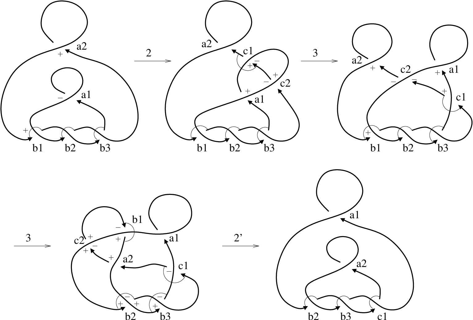
Figure 7 shows the succession of four Reidemeister moves. Using Theorem 4.1 it will be very easy to check that all four of them are possible; see Example 4.2. Note that we dropped primed labels from our notation which we hope will not lead to confusion. Let us compute the images of the cycles , , and under the composition of the four holonomies. (We could apply the chain maps to and as well but because those are not cycles in the chain complex (see Example 2.14), the results in themselves are not very informative. Let us just mention as an illustration that under the first of the four moves, the image of is .)
The first move is of type II. But because after the move, the diagram still only contains crossings with grading or ( and ) and , the boundary of either one of the index crossings , , and is still after the move. Thus by Proposition 3.5, all of them are mapped trivially. The two type III moves that follow only affect () but this is not relevant for our purpose. Finally, the holonomy of the II-1 move takes to (and to ).
Next, we prove that a non-trivial monodromy implies that the loop itself is non-trivial.
3.2 Chain homotopies
It is a folk theorem of singularity theory (see for example [1, p. 18], where the more general situation of plane curves with semicubical cusp singularities is considered) that there are six different codimension strata (bifurcations) of degenerate immersions of –manifolds into –manifolds. These are the three different possibilities of two distant Reidemeister moves happening at the same time, and three more types: quadruple points with pairwise transverse branches; degenerate triple points when exactly two branches are tangent; and cubic tangency of two branches. The neighborhoods (versal deformations) of points on each of these strata are also understood (see [1, Figure 6]).
For our purposes, each case has to be further separated according to the actual position of the branches in –space. Thus, we have six types of quadruple points corresponding to the six cyclic orderings of the branches. Degenerate triple points have three types distinguished by whether the third branch crosses over, under, or between the two whose projections are tangent. Cubic tangencies are separated into two obvious types. As to the cases of simultaneous Reidemeister moves, let us note that if two degenerate Reeb chords appear at the same time, their lengths, which we’ll call the height of the move, can generically be assumed different.
Theorem 3.7.
Let be a Legendrian knot type. Let and be generic elements of and , two generic paths joining them, inducing the holonomies . If these paths are homotopic with their endpoints fixed, then .
Proof.
As and are homotopic, there is also a generic homotopy connecting them. This map meets the codimension discriminant transversely in finitely many points. If the number of such points is zero, then the only time the sequence of Reidemeister moves changes is those finitely many values of when is tangent to (for some value of ). At these instances, a pair of Reidemeister moves appears or disappears. Because these two moves are inverses of each other, their holonomies cancel each other out by what we have shown in the proof of Theorem 3.2. The rest of the proof consists of an analysis of the codimension strata of the discriminant, as described in the introduction of the section.
Case 1\quaSimultaneous Reidemeister moves where the two or three crossings affected by the moves form disjoint sets (“far away” moves)\quaEach such case fits the scheme (differentials noted for reference later)
| (11) |
and we can arrange that if one or two pairs of Reidemeister II, II-1 moves are involved, then the arrows always point in the direction of the II-1 move. Then it suffices to check that in each case, the two compositions of chain maps from upper left to lower right agree. Therefore it will not be necessary to introduce a chain homotopy, or in other words, it can be chosen to be . This phenomenon will re-occur in each case except the very last one.
By our last assumption and the formulas of Theorem 3.2, the claim is clear for generators not directly affected by the moves. If any of the moves is a triangle move, it is straightforward to check for the vertices of the triangle, too. Suppose the horizontal arrows represent II-1 moves, with disappearing crossings and , so that . The crossing gets mapped to under either composition. Let . Then and . But because and hence , and , we have . So to show that , we need to prove that1111 11 Note that, with a slight abuse of notation, we sometimes suppress the chain map relating DGA’s of different diagrams when it simply replaces all generators in one expression by corresponding generators from the other diagram. Our “excuse” is that these new generators are denoted by the same symbols as the old ones. A more exact version of the claim would be that and are expressed by identical polynomials in the two DGA’s. . This follows by a case-by-case analysis. If and are induced by triangle moves then they clearly act the same way on . If it is a II-1 move with a bigger height than that of the one inducing , then . If the height is lower than that of the first move, then we have to make sure that the same expression computes the boundary of the higher-index vanishing crossing of the second move in each diagram of the upper row of (11), because this is used to define and . But this is clear since is a chain map and the expressions in question can’t contain neither nor .
Case 2\quaQuadruple points\quaWe are going to draw circles linking the singularity once and compute monodromies around these loops, starting and ending at the top left in each of the cases depicted in Figures 9 and 10. Such a loop meets the triple point discriminant eight times and in each case we will find that the composition of the corresponding eight chain maps is the identity.


Out of the six cases, the one on the bottom of Figure 9 is the most complicated, due to the fact that all eight moves are of type III. Even in this case, only the crossings , , and need checking, because others are always mapped trivially. On the left side of Figure 9, we indicated the orientation signs used in the following. In the second move, ’s image is . The three generators in this expression are mapped trivially until the sixth move, when the image becomes (this is by the same argument applied in the proof of Theorem 3.2). The generator returns to itself through two completely analogous moves. Finally, we have the following for :
The equality stated in the fourth row, as well as the very last one, holds by the argument in the proof of Theorem 3.2. The other one in the sixth row is true because
- •
and both equal the total winding of , with each capping path thought of as starting and ending at the quadruple point.
- •
by Lemma 2.3.
The other five quadruple point bifurcations can be handled with very similar, and simpler, computations.
Case 3\quaDegenerate triple points\quaFor the three bifurcations on the top of Figure 8, we claim that the chain maps corresponding to the two ways of moving from upper left to lower right in the diagrams induce the same chain maps. Please refer to Figure 8 for the positions of the orientation signs that appear in the calculations and note that and always denote orientation signs of opposite quadrants. Consider the third case (middle of Figure 8). Denote the differential of the upper left diagram by , of the lower left diagram by and that of the upper right diagram by . Applying the chain maps of Theorem 3.2 to the generator , we find the following:
Here, and are defined by the equations and . The coefficients of agree in the two images of by Lemma 2.3 and the observation that the capping paths and used to compute the exponents of coincide at the moment of self-tangency. Thus, we need to prove that . For this, note that and , therefore , which is also the expression of . Now, follows because . The claim is clear for other generators of the upper left diagram.
In the other two cases (top row of Figure 8), the proof is very similar. It is important to note though that in the first diagram of the top row, , and in the second, in a neighborhood of the codimension discriminant. Due to this fact, the boundary of is given by the same polynomial in both pairs of upper right and lower left diagrams.
Case 4\quaCubic self-tangencies\quaNote that on the two remaining diagrams (bottom row of Figure 8), we only have two Reidemeister moves; the chain maps and are simple re-labelings. In the case depicted on the second diagram, we still don’t need to introduce a non-zero chain homotopy. This is because , (it is an easy fact that ), and a similar computation for .
Finally, it is the situation on the bottom left of Figure 8 which does require a non-trivial chain homotopy , mapping between the two indicated DGA’s. Let and let map all other generators to . We extend as in Lemma 2.18. Let and . Then , and , where the polynomials and are defined in the upper left diagram by the equations and . Finally, it is easy to check the following, too:
(because doesn’t contain );
(because ), and
where, indeed, and . ∎
3.3 –coefficients
In this subsection we briefly summarize the modifications needed to reduce our discussion to the original –coefficient theory of Chekanov. (We will work in that context in sections 6 through 10.) Please note again that this means that we are going to describe the same geometry (Legendrian knots, their families, Reeb chords, and holomorphic discs) using slightly less sophisticated algebra: The generators are still the same Reeb chords, ie crossings, and the product is non-commutative, but we substitute , reduce integers modulo , and reduce the grading modulo , where is the common Maslov number of each knot in the family. The only simplification we get in Table 1 is that now, (and ). Otherwise, we keep all notation introduced in this section and still refer to Figure 6 (orientation signs can now be ignored).
A list of maps that, when extended from the generators to the DGA as algebra morphisms, become the chain maps that are used to define holonomies and monodromies of (sequences of) Reidemeister moves, is as follows.
Move III: Let , , , and , where is any other crossing of the upper diagram.
Move III: Let
while other generators are mapped trivially: , , and .
Move II-1: Let . Define , which gives rise to the obvious re-labeling . Then let
Move II: The map still takes
for all . Formula (9) of Remark 3.4 becomes
and formula (10) takes the form
In the rest of the paper, each time we compute the holonomy of a Reidemeister II move, Proposition 3.5 applies. In other words, the detailed description of move II was included only for completeness.
4 Legendrian Reidemeister moves
In this section, we investigate a very basic question, which arises naturally in the theory of Legendrian knots and links. The question is this: if a Lagrangian diagram of a Legendrian link contains a part that is topologically fit for a Reidemeister II, II-1, or III move, can we carry the move out in the Legendrian category? (If so, we will call the move consistent.) As it turns out, the answer is not always affirmative and a necessary and sufficient condition can be formulated in terms of a linear program.
We call two regions (of the complement of a knot diagram) adjacent at a vertex if they share the vertex (crossing) but don’t share any edges.
Theorem 4.1.
Each Reidemeister move of Figure 6 is possible if and only if the Lagrangian diagram can be isotoped (in the Legendrian sense) so that a certain inequality is satisfied. The list is as follows:
- •
Move III: the area of the triangle is smaller than the area of any of the three regions adjacent to it at either of its vertices.
- •
Move III: the area of the triangle is smaller than the area of the region adjacent to it at the vertex .
- •
Move II-1: the area of the –gon is smaller than the sum of the areas of the two regions adjacent to it at its vertices.
- •
Move II: the sum of the heights of the crossings along the right side of the pinching region, counted with Reeb signs, is positive. (If the region to the right of the pinching, as it is depicted in Figure 6, is the unbounded one, then there is no obstruction to the move.)
Recall from section 2 that every Lagrangian diagram has the non-empty cone associated to it. is defined by the positivity constraints on the heights associated with and finitely many homogeneous linear inequalities (coming from bounded regions of the complement) in terms of these heights (see Remark 2.5). Each inequality of Theorem 4.1 requires that a certain linear objective function1212 12 The objective function is linear exactly because the areas of the regions are linear functions of the heights. These areas can also be thought of as slack variables. defined on take on a positive value. That is, in each case the necessary and sufficient condition can be re-phrased to require that a certain linear programming problem be unbounded. This can be checked by the simplex method or any other linear programming algorithm (for small diagrams even by hand, as the author can attest).
Proof.
The “only if” part of each statement is easy to justify. To see this for move II, use Proposition 2.2: at the moment of self-tangency of the projection, the sum in question is the area of the region pinching off on the right side plus the difference in –coordinate between the two preimages of the self-tangency. As this is positive, our sum must have been positive for some period of time before the move happened, too. The other three moves involve the vanishing of the area of a region; clearly, for some time before that happens, the particular area is smallest among all others and the said inequalities hold.
Now to prove the “if” statement for move II, suppose that the sum described in the statement is positive and extend a very narrow ‘finger’ that follows closely the right side of the region from the lower edge to the upper one. The area of the finger can be made arbitrarily small and therefore with a slight downward bump on the lower edge (see Remark 2.8) we can make sure that other parts of the knot (in particular the value of ) are not affected. As we are also able to arrange that the area that is pinching off be less than , an application of Proposition 2.2 shows that at the moment the finger reaches the upper edge, it must do so so that it crosses underneath it. If the ‘right side’ that we used doesn’t exist due to the unboundedness of the pinching region, then simply let the finger follow a path that encircles a large enough area (on the finger’s left) so that it dips down sufficiently.

In the other three cases, we again utilize the idea described in Remark 2.8. To carry out move III, replace the uppermost strand as indicated in Figure 11. It is clear from the proof of Proposition 2.2 that if the new arc, starting from the old crossing , follows the side close enough, then the new crossing has height arbitrarily close to , and is arbitrarily close to . In particular, the types of the crossings are as indicated. Then, if we followed the sides and close enough, we can use the excess area of the region to compensate for the modification.
Three very similar arguments establish the claim for move III, and Figure 12 is self-explanatory for the case of move II-1.∎

Example 4.2.
We’ll prove that the loop of trefoils in Example 3.6 is sound, ie, all four of the indicated Reidemeister moves can indeed be carried out. Let us consider the first diagram in Figure 7. By adding “bulges” of equal area to the regions that were denoted by and in Figure 4, we may arrange that the areas of those, along with the height , be arbitrarily larger than any other area or height occurring in the projection. In particular, can be made positive, which by Theorem 4.1 means that the first move is possible. The triangle move that follows is consistent because the region adjacent to the triangle at is the unbounded one. At this point, we may finish the argument by pointing out that the remaining two moves are mirror images of the first two, or we may continue as follows: For the other triangle move, enlarge the areas of the triangle and of the region capping off until the area of the triangle gets bigger than that of the triangle (this is meant in the third diagram of Figure 7). Finally, the same trick applied to the bounded regions adjacent to in the fourth diagram makes sure that the appropriate condition from Theorem 4.1 is satisfied and the last move of the loop is consistent, too.
5 First evidence of non-triviality
At this point we are ready to prove that the monodromy invariant of Theorem 1.1 is non-trivial. We will use essentially the same example to establish Corollary 1.4, too.
Note that the first and last diagrams of Figure 7 coincide, so in Examples 3.6 and 4.2 we investigated a loop of Legendrian trefoil knots. It is not hard to identify it with (defined in the introduction). If we re-label the fifth diagram like the first one, we can write that the monodromy of the loop (which is the composition of the four holonomies of Example 3.6 and the re-labeling) acts on the cycles , , and as follows:
Proposition 5.1.
Proof.
As and , all three generators are on the same orbit. Then we compute that and that
The argument for the order will be complete if we show that in the homology, ie, that there isn’t an element so that . For this, notice that is contained in the two-sided ideal generated by and . An examination of equations (3) and (4) shows that after substituting , they both contain an even number of terms that are powers of (namely, two and zero terms). Therefore the same property holds for the entire ideal. Since is not such a polynomial, it cannot be in the image of the differential. ∎
It is easy to see that if we fix the basepoint, but allow knots in our one parameter families that are not Legendrian, then the three-fold concatenation of is homotopic to a continuous rotation by radians. Therefore, as is generated by exactly this loop, the six-fold concatenation of is contractible in the space of smooth right-handed trefoil knots. But because (as ), is non-contractible in the space of Legendrian trefoil knots. This last implication, which establishes Corollary 1.4, holds by Theorem 3.7. (We remark that with a bit of extra work, it can be shown that is itself contractible in , so taking its sixth power isn’t really necessary in our argument.)
In sections 9 and 10, we will generalize the proof of Proposition 5.1 for an arbitrary torus knot. (Except that to simplify the discussion, in those sections we will work with –coefficients.) Before we do that, we use sections 6 and 8 to set up a more general picture. Section 7 contains a vital ingredient of the proof of Theorem 1.3.
6 Positive braid closures
Let us consider a positive braid on strands, as in Figure 15. Label the left and right endpoints of the strands from top to bottom with the first whole numbers. The pair of left and right labels on each strand takes the form , where is the underlying permutation of . Further, label the crossings of the braid with a pair of numbers, the first one the left label of the overcrossing strand and the second one the right label of the undercrossing one. (Note that not all pairs of numbers between and occur as labels of crossings; for example, never does for any .)
Definition 6.1.
A positive braid defines the front diagram of an oriented Legendrian link as on the upper half of Figure 13 (orient each strand of from left to right). We call this construction the Legendrian closure of and denote it by .

Note that the types of crossings are correctly determined by the slopes of the branches that meet there exactly because the braid is positive. Applying Ng’s [23] construction of resolution to the front diagram, we obtain the Lagrangian diagram in the lower half of Figure 13.
In section 2, we omitted the modifications needed to define the invariants (such as rotation and Thurston–Bennequin numbers and contact homology itself) for oriented multi-component Legendrian links. We include an informal rundown here (see [23, section 2.5] for more). The rotation number is the sum of the rotations of the components. The Thurston–Bennequin number is still the writhe of the Lagrangian projection; note that now, as opposed to the case of a single component, the orientation matters in its definition.
From now on, we will always use –coefficients in contact homology. For a multi-component link, there is not a single distinguished grading of its DGA, rather a family of so called admissible gradings. We consider those introduced in [23] and not the larger class of gradings described in [6, section 9.1]. In the –coefficient theory, each of these is defined modulo the greatest common divisor of the Maslov numbers of the components (recall that the Maslov number is twice the rotation number of a knot). Self-crossings of individual components have the same well-defined index in any admissible grading. We will refer to such generators as proper crossings. Other crossings’ indices have the same parity in each admissible grading. The parity of the index of any crossing coincides with its sign in classical knot theory.
The differential is of index with respect to each admissible grading. (Furthermore, Lemma 2.3 holds for each admissible grading, too.) Contact homology is a well-defined invariant in the sense that if two diagrams are Legendrian isotopic, then there is a one-to-one correspondence between their sets of admissible gradings so that the corresponding contact homologies are isomorphic as graded algebras.
It is easy to calculate that the Legendrian closure of any positive braid has rotation number (in fact, every component has Maslov number ). The Thurston–Bennequin number is . The positive Legendrian torus knot obtained as a special case is the one with maximal Thurston–Bennequin number (see [11] for a classification of Legendrian torus knots). The torus knot that we considered earlier arises from this construction, too. The unique Legendrian unknot with maximal Thurston–Bennequin number [3, 8] is the Legendrian closure of the trivial braid on a single strand.
In the Chekanov–Eliashberg DGA of , the grading (any admissible grading) is integer-valued. The crossings () have index . The rest of the generators are the crossings of and they have index . In the multi-component case we should say instead that the grading that assigns the index to each is admissible; from now on, we will always work with this grading. These generators will be labeled by , where the integers are the ones defined at the beginning of the section. The third label is used to distinguish between multiple intersections of strands, enumerating them from left to right, as shown in Figure 14.

Since lowers the index by ,
In fact, there are no admissible discs whose positive corner is an index crossing. The boundaries , , are polynomials in the non-commuting variables only. Our goal for the remainder of this section is to compute these polynomials.
The first observation is that for all , there is an admissible disc covering the teardrop-shaped region right above once. We’ll call it the trivial disc. It contributes to . The trivial disc is the only one that turns at the upward-facing positive quadrant at . The rest of the contributions to come from discs that turn at the positive quadrant facing down.
Suppose is an admissible immersion with respect to the projection , with positive corner and so that it is different from the trivial disc. Fix points on as shown in Figure 13.
Lemma 6.2.
The curve doesn’t pass through the points .
Proof.
In fact, if we denote the region of the complement directly under by , then is disjoint from , as well as from . To see this, first shrink so that all areas and heights are smaller than , where is to be chosen later. Then add “bulges” of equal area to and on the outside of the diagram (see Remark 2.8). Next, add bulges of area to and on their sides facing . Continue all the way until adding bulges of area to and on their sides facing . The result is a Lagrangian projection of the same link in which, after the choice of a small enough , the claim is obvious by Lemma 2.11, except for the case of . But that follows from the easy observation that if any admissible disc passes through so that locally, faces downward, then is the trivial disc. ∎
Recall that is oriented as shown in Figure 13. We have already noted that apart from its positive corner which is of index , turns only at certain index crossings . By Lemma 2.10, this implies that is compatible with the orientation of . Therefore, as the orientation of agrees with that of near the positive corner , these orientations agree at all points of . This last observation for example implies that can’t turn at the downward facing negative quadrant at any of the ’s.
We may summarize our findings about so far as follows. The curve starts at , follows until it reaches the braid at the left endpoint labeled (while extends this map toward ). Then it travels through the braid, possibly turning (left) at several crossings but always heading to the right, until it reaches a right endpoint labeled . Then climbs to and, unless , beyond (note that can’t have a positive corner at ) to , at which point the extension is toward . Then descends back to so that it doesn’t turn at the negative corner. So the process repeats with replaced with (where ), and so on until for some .
Definition 6.3.
A finite sequence of positive integers is called admissible if for all , between any two appearances of in the sequence there is a number greater than which appears between them. For , let us denote by the set of all admissible sequences that are composed of the numbers .
For example, , , and
By induction on and observing the position of the unique maximal term in the sequence, it is easy to prove that .
Proposition 6.4.
For the admissible disc as above, the sequence of intermediate labels is an element of .
Proof.
There is an intuitive reason for the claim: if the index was repeated without the boundary of the disc climbing higher between the two occurrences, then the disk would pinch off at . We shall give a more rigorous proof using Blank’s theorem (see [24], or the review in [17], from where we’ll borrow our terminology).
Let be a small generic perturbation of . This has the corners rounded so that is an immersion; moreover, let us note that because may cover parts of more than once, the complement of typically contains more regions than that of . We are going to apply Blank’s theorem to . We extend rays from each bounded component of to infinity. If the region is not one of those obtained from the (let us denote these by ), or one of the small ones resulting from perturbation close to the arc bounding , this can be done so that only intersects the ray in a positive manner (ie, if the ray is oriented toward , then crosses from the right side to the left side). By our observation on the compatibility of , this implies that also intersects those rays positively. Let us draw rays starting from the regions as in Figure 13. Label all rays, in particular label these last with the symbols .
The Blank word of the disc is obtained by tracing , starting from, say, , and writing down the labels of the rays we meet with exponents according to positive and negative intersections (we’ll call these positive and negative symbols or letters). A grouping of the Blank word is a set of properly nested disjoint unordered pairs of the form so that each negative symbol is part of exactly one pair. Blank’s theorem states that the set of groupings of the Blank word is in a one-to-one correspondence with non-equivalent extensions of the immersion to immersions of .
As is such an extension, a grouping exists and we claim that this implies the Proposition. We delete labels different from the from the Blank word of and concentrate on the remaining word, which also inherits a grouping (note that most of the deleted labels only appeared positively anyway, except for certain ones that belong to some regions that were the result of perturbation). We’ll call this the Blank word of and denote it by . Note that if we only keep the negative letters from , then the sequence of their indices is exactly . In fact, is decomposed into segments ended by these negative symbols, and a final segment :
We’ll prove the following statements by induction on :
- (1)
Each copy of is paired in the grouping with a copy of which is located to the right of it.
- (2)
None of the pairs is nested in a pair for any .
- (3)
Any two copies of are separated in by a copy of for some .
The last statement of course directly implies the Proposition.
The last letter of is and this is the only positive occurrence of this letter. Hence (1) and (2) are obvious for . Also, since a second one wouldn’t find a pair, there can be at most one copy of in , thus (3) is vacuously true for .
Assume that the statements hold for all . To prove (1), assume that a certain copy of forms the pair with a copy of , which is to the left of it. Then, as can’t be part of the final segment , it belongs to some with last letter , where , ie . This copy of is to the left of , hence it is part of a pair which is nested inside , which contradicts the hypothesis (2) for .
To prove (2), suppose that a certain pair is nested in where has an index less than . This copy of can’t be part of because it has a symbol with lower index (namely, or ) to the right of it. It is clear then that the first negative letter after has index , which is higher than (ie ), and it is still nested in . Then so is the pair containing it, which contradicts (2) for .
Finally for (3), assume the contrary again, namely that there are two copies of in that are not separated by any higher index negative symbol. Then the pair of the first can not lie between them either, because it would be part of some and then would separate. Thus, we have two pairs of the form nested in one another. But then the positive symbol of the inner pair would be followed by some , which is part of a pair that is nested in the outer pair, and that contradicts (2) for . ∎
Definition 6.5.
Let . The element of the DGA of is the sum of the following products. For each path composed of parts of the strands of the braid that connects the left endpoint labeled to the right endpoint labeled so that it only turns at quadrants facing up, take the product of the crossings from left to right that it turns at.
For example, contains the constant term if and only if . We will need the following polynomials of the :
Definition 6.6.
Let and let
Similarly, for , let
| (12) |
Finally, for any and , let
In particular, for each summand in , is the last element of the admissible sequence but it may occur elsewhere, too. For example, , , and . Note also that , , and , whenever these expressions are defined.
Theorem 6.7.
. Consequently, the index part of the contact homology has a presentation where the generators are the crossings of and the relations are for .
Proof.
The in the formula comes from the trivial disc. We claim that the rest of the contributions add up to . From Proposition 6.4 and the paragraph preceding Definition 6.3, we know that there can’t be any such terms other than the ones included in . To see that all such monomials actually arise from admissible discs, we just need to find those discs. This can either be done by an inductive construction on (for the inductive step, remove the smallest number from the sequence), or by applying Blank’s theorem. ∎
It is not clear whether contains any non-zero higher index part at all (except for the case of the unknot, when the single index crossing is a non-nullhomologous cycle). This is mainly why we only work with in this paper. This difficulty in handling contact homology also underlines the importance of the augmentation that we construct in the next section.
7 Augmentations of braid closures
Definition 7.1.
An augmentation of the Lagrangian diagram of a Legendrian link is a subset of its crossings with the following properties.
- •
All elements of are proper crossings of (ie, intersections of different components are not allowed in ).
- •
The index of each element of in any admissible grading is (in fact, this requirement implies the previous one).
- •
For each generator , the number of admissible discs with positive corner and all negative corners in is even.
The last requirement implies that the evaluation homomorphism (which is defined on the link DGA, and which is also called an augmentation) that sends elements of to and other generators to , gives rise to an algebra homomorphism .
Example 7.2.
Remark 7.3.
Let us return to the front diagram in the upper half of Figure 13. Such a diagram always has an admissible decomposition (or ruling) in the sense of [5]: the only two values of the Maslov potential (even though it’s –valued) are on the upper strands and on the strands of the original braid , thus all crossings are Maslov, and we may declare all of them switching (in the multi-component case, consider only proper crossings). This gives rise to a decomposition where the discs are nested in one another, so it’s admissible.
The existence of a ruling implies that is not a stabilized link type for any positive braid [5]. Also, by a theorem of Fuchs [18], it implies that the diagram has an augmentation1313 13 Fuchs and Ishkhanov [19] and independently Sabloff [25] have also proven that the existence of an augmentation implies the existence of a ruling. (note this is by no means unique). In his proof, Fuchs constructs an augmentation of a diagram which is equivalent to the original but has a lot more crossings. This means that the original diagram can also be augmented: the pull-back of an augmentation by a DGA morphism, like the ones listed in section 3.3, is again an augmentation.
In the case of a braid closure, it would be impractical to pull back Fuchs’ augmentation to the original diagram. Instead, we’ll start from scratch and construct an augmentation of the Legendrian closure of an arbitrary positive braid . When selecting crossings into , it will suffice to work with the braid itself, as illustrated in Figure 15, for the index proper crossings of are all crossings of . (We will call these the proper crossings of the braid .)

First, we associate an oriented graph to an arbitrary permutation . Let be one of the cycles of . Let us write the elements of around the perimeter of a circle in the cyclic order suggested by , directing an edge from to for all . (See Figure 15 for an example. The permutation in the diagram is the one underlying the braid). If is a non-maximal element of , then follow the cycle in the forward direction starting from until it hits the first number in which is bigger then . Let be the number immediately before that. In particular, . Do the same in the backward direction, resulting in the number such that . (For example, in Figure 15, is an element of a –cycle , with and .) Then, connect to by a directed chord of the circle and label the chord by . If , then instead, we attach a loop edge (labeled ) at to the graph. This will also be called a chord. Draw this loop edge inside the circle, right next to the perimeter, on the side of where the smaller of its two neighbors lies.
Definition 7.4.
If is non-maximal in its cycle , then the oriented loop that starts from , goes along the circle of to , then goes to on the chord labeled , then follows the circle again back to will be called the loop of . If is the largest number in , then let the loop of be the loop that travels around the original circle once.
Lemma 7.5.
If , then
- (a)
doesn’t contain
- (b)
the discs bounded by and are either disjoint or the latter contains the former.
In particular, the (oriented) chords obtained in the construction are pairwise disjoint. They can’t be parallel to the original edges and they differ from each other as well.
Proof.
Chords differ from edges because it’s impossible that each end of an edge be smaller than the other end (a chord and an edge can be parallel in the non-oriented sense, as in Figure 15). The other statements follow from (a) and (b). Statement (a) is obvious from the construction, and so is (b) if is maximal in .
The directed arc of the circle stretching from to only contains numbers less than . If this arc is disjoint from , then of course so is . Otherwise, the whole arc must be contained in . From this, statement (b) is clear, except if the chord labeled is a loop edge and either or . In the first case, , but , so (b) holds by the construction of the loop edge. The other case is handled analogously. ∎
Definition 7.6.
Let be the disjoint union of the graphs constructed above over all cycles of . This oriented planar graph, with vertices labeled by the numbers , is called the augmented graph of the permutation .
Lemma 7.7.
For all , the loop of is the unique directed loop in starting and ending at so that the sequence of the vertices (apart from ) visited by it is in .
Proof.
It is enough to prove the statement for a connected component associated to a cycle . The loop has the required property for all , because all the vertices visited by it are less than and no repetition occurs.
We have to rule out the existence of other loops. Since and are larger than , by the disjointness statement in Lemma 7.5, all loops in question are trapped in the disc bounded by (and this is obviously true when is maximal in ). Then by statement (b) of Lemma 7.5, apart from edges of , they may only contain chords labeled by numbers less than . Now, if the chord labeled by occurred in the loop and was the smallest such number, then because is not on , the sequence of vertices on would appear as a subsequence of the original vertex sequence of the loop. In that case, would be repeated in the sequence without the two occurrences separated by a larger number, which is a contradiction. ∎
The following “edge reversal lemma,” which we will need in section 10, can be proven very similarly.
Lemma 7.8.
For any so that , if is the second largest vertex (after ) along , then there is a unique oriented path in from to so that the sequence of the intermediate vertices is in . Otherwise, there is no such path.
Definition 7.9.
Let be a set of crossings of the positive braid . By the graph realized by we mean the oriented graph with vertices so that a directed edge connects to if and only if . Here, is as in Definition 6.5 and by we mean the element of obtained by substituting for elements of and for other generators in .
Lemma 7.10.
Let be the underlying permutation of and a set of proper crossings of . If the graph realized by agrees with the augmented graph of , then is an augmentation of the Legendrian closure of .
Proof.
Next, based on , we construct a candidate , and then we will use Lemma 7.10 to prove that it’s an augmentation. Loosely speaking, the edges of connecting to are always realized, even by the empty set. To realize the chord labeled , we’ll select the crossing into . We can do this because it always exists: (for left labels) and (for right labels), therefore the strand connecting to always meets the strand connecting to . If there were more than one points with the first two labels , we could have selected any of them1414 14 For instance, the crossing of Example 7.2 is denoted by in the general labeling system.; we used the third label for concreteness and for ease in the proof of Theorem 10.1. In Figure 15, we marked the selected crossings and labeled them with the label of the chord that they realize.
Proposition 7.11.
The set
is an augmentation of the Legendrian closure of the positive braid with underlying permutation .
In particular, for a pure braid , the empty set is an augmentation. In other words, the DGA of the Legendrian closure of a pure braid is augmented, ie, the boundary of each generator is a polynomial without a constant term. If is not pure, then , hence , and it follows that .
Proof.
It is clear from the construction that all the crossings in are proper. By Lemma 7.10, it suffices to prove that the graph realized by is the graph . For this, the chief claim is that no two points of are connected with a part of a strand so that it arrives at both points from above. In other words, the situation of Figure 16 can not arise: there is no pair of numbers so that . Indeed, then we’d have and similarly, , which would be a contradiction.

We know then that any path that is to contribute a non-zero summand to a certain can have at most one corner, which of course has to be in . Thus in the discussion before the Proposition we exhausted all such contributions: paths with no corners are responsible for the edges and paths with one corner are responsible for the chords of . So indeed, . ∎
Remark 7.12.
Let be the standard positive braid whose Legendrian closure is a positive torus link (the braid used to produce Figure 13 is an example with and ). If we apply our construction to it, we find an interesting connection of the resulting augmentation to the Euclidean algorithm. We mention this here without proof; we will only need a small part of the statement which is hidden in the proof of Proposition 10.3.
Let us denote the quotients and residues in the Euclidean algorithm (with input and ) as follows:
(Of course, .) The points of the augmentation are arranged in blocks of the following sizes: blocks of size ; blocks of size ; blocks of size and so on until the last blocks of size . If we draw the diagram of the braid as in Figure 17, every block can be viewed as the diagonal of a square, and the squares can in turn be seen to be placed inside a rectangular box so that they realize a ‘graphic implementation’ of the Euclidean algorithm.

8 A loop of positive links
Let be the Legendrian closure of the positive braid . Then there exists a natural closed loop in the connected component of the space of Legendrian links that contains , as follows. Let us write as a product of the braid group generators. In Figure 18, we show through an example how can be changed into the Legendrian closure of the conjugate braid that results from moving the first factor to the end of the word: if is a half-twist of the and strands of the braid, then one interchanges the and strands above the braid. In Figure 19, the same path is shown, but in the Lagrangian projection. Note that the index crossings and trade places. (The notation used on the diagram for the index crossings is the one that we will introduce below for the special case of torus links.) The Lagrangian diagrams of the endpoints are clearly obtained by resolution of the corresponding fronts. However, we will not prove that the paths themselves agree, too (up to homotopy). Instead, we will content ourselves with checking (using Theorem 4.1) that the four Reidemeister moves in Figure 19 are consistent, and thereafter use the Lagrangian construction as our definition of . (There are no such consistency issues with Reidemeister moves of fronts, but we need the Lagrangian diagrams to compute holonomies.)


Theorem 8.1.
The sequence of Reidemeister moves in Figure 19, defining , is consistent.
Proof.
This is a generalization of Example 4.2. Isotope the diagram just like in the proof of Lemma 6.2. Then by choosing a small enough , the height will dominate the expression whose positivity is needed (by Theorem 4.1) in order for the first move (which is a Reidemeister II move) to be consistent. To carry out the III move that follows, we need to isotope the second diagram from the top so that what remains from the region after the first move has larger area than the vanishing triangle. This can be achieved by the same trick (this time, moving away the ‘outer’ strands). Next, the newborn triangle needs to be blown up so that it has larger area than the triangle which is due to vanish in the second III move (which is the third move altogether). For this, the same trick with the bulges still works: apply it to the outer strands and the one that crosses itself at . Finally, the exact same argument guarantees that the fourth move, of type II-1, is consistent too. ∎
Let us use the formulas of section 3.3 to compute the holonomy of (cf Example 3.6). More precisely, we will compute the action of on the index crossings which generate the index contact homology . In the first move, two new crossings appear; using Lemma 2.3 it is easy to show that their indices are and . Let us denote the one with index by1515 15 In other words, let it inherit the labels of the crossing that is being moved to the other end of the braid. This is what we’ve done in Figure 19 too, except that there, a different notation is used for index crossings. and the one with index by . The old index crossings are not affected by this move (ie, the holonomy maps them trivially). This is true by Proposition 3.5: for index reasons, the boundary of any index crossing is . It is easy to see that the following two triangle moves don’t affect the old index crossings, either.
In the fourth, Reidemeister II-1 move however the crossing (together with ) vanishes, and its image in the holonomy becomes the polynomial . We used primed symbols to remind us that these are to be computed with respect to the conjugated braid. The fact that for each admissible disc that turns at the positive quadrant at that faces away from , the intermediate sequence of labels (of other index generators through which the boundary of the admissible disk passes) doesn’t contain any number larger than can be shown just like in the proof of Lemma 6.2. The fact that the sequence is admissible follows by an argument very similar to the proof of Proposition 6.4. Finally, the fact that each such admissible sequence does contribute the said terms can be established as in the proof of Theorem 6.7. We have proven:
Proposition 8.2.
The holonomy of maps each crossing of the braid trivially except the first one from the left, which is mapped to the polynomial (if the first crossing is between the and strands). This expression is to be computed as in Definition 6.6, with respect to the conjugate braid .
Note also that at the end stage of each crossing of the (conjugate) braid has index , thus in the multi-component case our choice of preferred grading is justified.
Now, it is clear that the concatenation is a closed loop in and by definition, its monodromy is the composition of holonomies , followed by a re-labeling to restore the original labels. Namely, each symbol labeling an index crossing needs to be changed back to ; in fact, would have to be changed to , but because we only concern ourselves with , this can be ignored.
9 divides
The last two sections of the paper contain the proof of Theorem 1.3. The argument works for any except when divides (the case of a pure braid), or divides . The reason why we don’t claim Theorems 1.3 and 1.2 for multi-component torus links is that we only proved Theorems 3.2 and 3.7 (and thus Theorem 1.1) for knots. (However, the extension of those proofs should only be a matter of changing the formalism to that of link contact homology.)
Let us revisit the loop of Legendrian torus knots defined in the introduction. As the braid is now composed of periods, the general loop described in section 8 is the -fold concatenation of another, and the latter is easy to identify as homotopic1616 16 Because we’ll omit the rigorous justification of this fact, the reader may treat the new description of as the definition. to . In particular, by Theorem 3.7, the ‘full’ monodromy takes the form , where is the monodromy of . From now on, we will concentrate on this map , and especially on its restriction to the index part of the contact homology of the standard torus link diagram (shown in Figure 13), representing the base point .
We will adjust our notation to this special situation. The crossings of will be indexed with two integers (as opposed to three), namely (, ) will denote the crossing counted from the top in the period of the braid. Note that in the definition of , after a full period of the braid has been moved from the left end to the right end, a re-labeling takes place, too: the second label of each crossing in the other periods is reduced by , and the labels in the now last period are changed to .
Proposition 9.1.
The monodromy of the loop of Legendrian torus links acts on the index generators as follows:
Proof.
The claim is clear for those crossings not in the first period: by Proposition 8.2, they are only affected, and in the described way, by the re-labeling. The rest of the statement will be proven by induction on . When this value is , ie , this is just the statement of Proposition 8.2 (the conjugate braid in this case is the original again, and the re-labeling changes into ). Assume the statement holds for . Right after the conjugation that removes it from the left end of the braid, the image of is , computed with respect to the braid after this conjugation. This can be re-written (by grouping terms with respect to the first factor in the product) as
where the terms labeled on the right are to be computed in the braid indicated by the box in Figure 19. Note however that by Definition 6.6, the same expressions are obtained if we use the whole braid (before re-labeling). If we apply the holonomies of the remaining conjugations and the re-labeling to this expression, we get (by the inductive hypothesis)
The last equality is true because the middle expression is exactly what results if we group terms in with respect to the last label in the admissible sequence which is more than . ∎
Proposition 9.2.
In the contact homology ring , we have:
| (13) |
| (14) |
and
| (15) |
We omitted and because they (and hence their images) are equal to in the contact homology. Recall also that and .
Proof.
When , none of the terms in contains any of , so they only need to be re-labeled. This means that all crossings that the path through the braid which generated the term turned at, are shifted to the left by a unit. This operation changes the entry point from the one labeled to the one labeled . If , then the shifted path can be completed by the overcrossing strand of the last period of the braid, which shows that the re-labeled expression is a summand in . Moreover, all such summands are obtained in this way exactly once. When , the re-labeling results in a summand of , but not all such are obtained: we miss contributions from paths that turn at the crossing (the last one on the strand with right endpoint ) . Hence the correction term in the top row of (13) (note that the paths turning at are exactly those that would otherwise have arrived at ).
When and , we have
Here, is the sum of the contributions to that don’t contain crossings of the first period. These terms only have to be re-labeled and that can be done just like in the argument above for when . In the sum of sums
we re-grouped the terms; those with an admissible sequence of labels formed , and the rest, where was repeated ‘illegally,’ formed .
Theorem 9.3.
The order of the (restricted) monodromy of the loop of Legendrian torus knots divides .
Proof.
This is now a straightforward computation, generalizing the first paragraph of the proof of Proposition 5.1. Consider the generator (). By Proposition 9.1, the first iterations of act on it as follows:
Then by (14) of Proposition 9.2, the next iterations are as follows:
Now by (15), the next iterations are
Finally, because , (13) yields
Because is on the orbit of for all , we see that is the identity on all of the degree generators. ∎
10 divides
Theorem 10.1.
The number divides the order of the monodromy .
In the proof of Theorem 9.3, we described explicitly the -element orbit of each index generator (altogether orbits). Recall that all of those orbits contain a –sequence of length , a –sequence of length and an –sequence of length . (These expressions are cycles in the chain complex , but we really mean the homology classes represented by them.) We will choose one of these orbits and show that it doesn’t have a period shorter than . For this, we will evaluate the augmentation (see Proposition 7.11) on elements of the orbit, and prove that the resulting sequence of ’s and ’s, which we will call the -–sequence of the orbit, has no such shorter period. In fact, we claim the following:
Proposition 10.2.
If but , the -–sequence of the orbit of consists of consecutive ’s and consecutive ’s. If but , then the same holds for the orbit of .
In the latter case, we will denote the value by . For the rest of the section, either this value or , as the case may be, should be substituted for in the formulas for the –, –, and –sequences. Note that if , the said orbit doesn’t even exist (if and , then its -–sequence consists only of ’s).
Recall that was constructed so that the graph realized by was the augmented graph of the underlying permutation of the braid. Hence, this oriented graph has adjacency matrix and therefore it contains all the information we need to evaluate the algebra homomorphism on the polynomial expressions of the – and –sequences. We will only need to refer to the actual braid in the case of the –sequence. In our situation,
When , we could equivalently write . This explains why our choice of orbit in Proposition 10.2 is reasonable: both in the –sequence and in the –sequence the two lower indices are always the endpoints of an edge of , but they are listed in the reverse order. So when we evaluate on these polynomials, what we need to examine is whether the given edge of the graph can be “reversed,” ie, if it is part of an oriented loop (and how many loops) with an admissible sequence of vertices.
We will re-state and prove Proposition 10.2 in a more detailed version.
Proposition 10.3.
The orbit specified in Proposition 10.2 contributes ’s and ’s to the sequence as follows.
- (1)
If but (hence in fact ), then we have
- (2)
If but , then the sequence is
- (3)
If , , and , then we get
- (4)
Finally, if , , and , then we have
Proof.
–sequence\quaIn case (1), all numbers are so that and . This means that , ie, that there is a loop edge attached to in . It is easy to check that in the construction of , the crossing that realizes this loop edge is exactly .
In case (2), we similarly find loop edges but only attached to the numbers . These are realized by the crossings . For the crossings , we find that their second labels in the system that we used to label crossings of general braids in section 6 are also . These numbers can not be the endpoints of a chord because the numbers preceding them in the permutation (namely, ) are smaller than them. Therefore these crossings are indeed not selected into .
In cases (3) and (4), first note that the crossings have third labels greater than in the labeling system of section 6, so they never get selected into . Neither do , because their ‘old’ first labels are and these are taken to the smaller values by (ie, they’ll never be the startpoint of a chord). After this, the rest of the –sequence can be sorted out just like in the first two cases.
–sequence\quaHere the claim is that it always contributes only ’s to . This is because implies . Indeed, since it is preceded in the permutation by a smaller number, can’t be the endpoint of a chord, only of the single edge coming from . So there is a unique term in that contributes to , namely the one which, when multiplied by on the right, produces the term corresponding to the unique loop described in Lemma 7.7.
–sequence\quaAll the four claims in this case follow from Lemma 7.8. Note in particular that if we allowed in case (1), then would be the second largest vertex on for all , and therefore the first elements of the –sequence wouldn’t be mapped to by . However if , then the first number after the sequence ‘wraps around’ the circle is different from . If is also smaller than (and this will be the case exactly when ), then it falls between and , so is not second largest in . If is larger than , then it is recognized as what we called in section 7. But then there exists a chord in , starting from , and ending at the element of . This is by construction such that . But because , if we assume that , then this is only possible if , ie if . This again means that in these cases, is not second largest on . This proves the claim about the first part of the –sequence. Finally, if (which implies ), then only visits the positive elements of the arithmetic progression (ie, there is no wrapping around) and is obviously second largest among these. Cases (2), (3) and (4) can be handled similarly. ∎
Note that this was a generalization of the second paragraph in the proof of Proposition 5.1; there, we used the augmentation .
References
- [1] V I Arnol’d, Invariants and perestroikas of fronts on a plane, Trudy Mat. Inst. Steklov. 209 (1995) 14–64 \MR1422217
- [2] C Benham, X-S Lin, D Miller, Subspaces of knot spaces, Proc. Amer. Math. Soc. 129 (2001) 3121–3127 \MR1840119
- [3] D Bennequin, Entrelacements et équations de Pfaff, from: “Third Schnepfenried geometry conference, Vol. 1 (Schnepfenried, 1982)”, Astérisque 107, Soc. Math. France, Paris (1983) 87–161 \MR753131
- [4] F Bourgeois, Contact homology and homotopy groups of the space of contact structures, \arxivmath.SG/0407531
- [5] Y Chekanov, New invariants of Legendrian knots, from: “European Congress of Mathematics, Vol. II (Barcelona, 2000)”, Progr. Math. 202, Birkhäuser, Basel (2001) 525–534 \MR1909953
- [6] Y Chekanov, Differential algebra of Legendrian links, Invent. Math. 150 (2002) 441–483 \MR1946550
- [7] T Ekholm, J Etnyre, M Sullivan, Legendrian submanifolds in and contact homology, \arxivmath.SG/0210124
- [8] Y Eliashberg, M Fraser, Classification of topologically trivial Legendrian knots, from: “Geometry, topology, and dynamics (Montreal, PQ, 1995)”, CRM Proc. Lecture Notes 15, Amer. Math. Soc., Providence, RI (1998) 17–51 \MR1619122
- [9] Y Eliashberg, A Givental, H Hofer, Introduction to symplectic field theory, Geom. Funct. Anal. (2000) 560–673 \MR1826267
- [10] J B Etnyre, Legendrian and Transversal Knots, \arxivmath.SG/0306256
- [11] J B Etnyre, K Honda, Knots and contact geometry. I. Torus knots and the figure eight knot, J. Symplectic Geom. 1 (2001) 63–120 \MR1959579
- [12] J B Etnyre, K Honda, On connected sums and Legendrian knots, Adv. Math. 179 (2003) 59–74 \MR2004728
- [13] J B Etnyre, K Honda, Cabling and transverse simplicity, e-print, \arxivmath.SG/0306330
- [14] J B Etnyre, L L Ng, J M Sabloff, Invariants of Legendrian knots and coherent orientations, J. Symplectic Geom. 1 (2002) 321–367 \MR1959585
- [15] Y Félix, S Halperin, J-C Thomas, Differential graded algebras in topology, from: “Handbook of algebraic topology”, North-Holland, Amsterdam (1995) 829–865 \MR1361901
- [16] A Floer, Symplectic fixed points and holomorphic spheres, Comm. Math. Phys. 120 (1989) 575–611 \MR987770
- [17] G K Francis, Extensions to the disk of properly nested plane immersions of the circle, Michigan Math. J. 17 (1970) 377–383 \MR0284985
- [18] D Fuchs, Chekanov-Eliashberg invariant of Legendrian knots: existence of augmentations, J. Geom. Phys. 47 (2003) 43–65 \MR1985483
- [19] D Fuchs, T Ishkhanov, Invariants of Legendrian knots and decompositions of front diagrams, Mosc. Math. J. 4 (2004) 707–717, 783 \MR2119145
- [20] A Hatcher, Spaces of knots, \arxivmath.GT/9909095
- [21] M Hutchings, Floer homology of families I \arxivmath.SG/0308115
- [22] M Hutchings, Floer homology of families II: symplectomorphisms, in preparation
- [23] L L Ng, Computable Legendrian invariants, Topology 42 (2003) 55–82 \MR1928645
- [24] V Poénaru, Extensions des immersions en codimension (d’après Samuel Blank), Séminaire Bourbaki, Vol. 10, Exp. No. 342, Soc. Math. France, Paris (1995) 473–505 \MR1610469
- [25] J M Sabloff, Augmentations and rulings of Legendrian knots, Int. Math. Res. Not. (2005) 1157–1180 \MRMR2147057
- [26] P Seidel, of symplectic automorphism groups and invertibles in quantum homology rings, Geom. Funct. Anal. 7 (1997) 1046–1095 \MR1487754