Skein theory for $SU(n)$ -quantum invariants

Adam S. Sikora Address: Department of Mathematics, University at BuffaloBuffalo, NY 14260-2900, USA Email: asikora@buffalo.edu

Abstract

For any $n\geq 2$ we define an isotopy invariant, $\left\langle\Gamma\right\rangle_{n},$ for a certain set of $n$ -valent ribbon graphs $\Gamma$ in ${\mathbb{R}}^{3},$ including all framed oriented links. We show that our bracket coincides with the Kauffman bracket for $n=2$ and with the Kuperberg’s bracket for $n=3.$ Furthermore, we prove that for any $n,$ our bracket of a link $L$ is equal, up to normalization, to the $SU_{n}$ -quantum invariant of $L.$ We show a number of properties of our bracket extending those of the Kauffman’s and Kuperberg’s brackets, and we relate it to the bracket of Murakami-Ohtsuki-Yamada. Finally, on the basis of the skein relations satisfied by $\left\langle\cdot\right\rangle_{n},$ we define the $SU_{n}$ -skein module of any $3$ -manifold $M$ and we prove that it determines the $SL_{n}$ -character variety of $\pi_{1}(M).$

keywords

Kauffman bracket, Kuperberg bracket, Murakami-Ohtsuki-Yamada bracket, quantum invariant, skein module

\primaryclass

57M27 \secondaryclass17B37

\agt

ATG Volume 5 (2005) 865–897\nlPublished: 29 July 2005

\thetitle

\theauthors

Abstract\stdspace\theabstract

AMS Classification\stdspace\theprimaryclass; \thesecondaryclass

Keywords\stdspace\thekeywords

1 Introduction

The $SU_{2}$ -quantum invariant of links, known as the Jones polynomial, can be conveniently defined in terms the Kauffman bracket invariant, [17]. This approach has several advantages, for example, leading to definitions of skein modules and Khovanov homology¹¹ 1 The Kauffman bracket skein relations allow a particularly simple definition of Khovanov’s $SU_{2}$ -homology groups, [36]. – two notions in the center of current active research – see for example [5, 9, 10, 12, 11, 30, 34] and [2, 3, 13, 15, 16, 19, 20, 21, 24, 31, 36]. In [23], Kuperberg constructs a bracket isotopy invariant of links and $3$ -valent graphs in ${\mathbb{R}}^{3},$ with properties analogous to those of the Kauffman bracket, and shows that it coincides with the $SU_{3}$ -quantum invariant. We extend his work, by defining a bracket isotopy invariant $\left\langle\cdot\right\rangle_{n}$ for any $n\geq 2$ and by showing that it determines the $SU_{n}$ -quantum invariant. More specifically, for any $n\geq 2$ we consider the set ${\cal W}_{n}({\mathbb{R}}^{3})$ of $n$ -webs which are ribbon graphs $\Gamma$ in ${\mathbb{R}}^{3}$ whose coupons are either $n$ -valent sources or $n$ -valent sinks. In particular, ${\cal W}_{n}({\mathbb{R}}^{3})$ contains all oriented framed links in ${\mathbb{R}}^{3}$ for any $n.$ We define a bracket isotopy invariant of $n$ -webs, $\left\langle\Gamma\right\rangle_{n},$ and show that it coincides with the Kauffman bracket for $n=2$ , and with the Kuperberg’s bracket for $n=3.$

For reader’s convenience, we state three different definitions of $\left\langle\cdot\right\rangle_{n}$ : by skein relations, (Theorem 1), by a state sum formula, (Proposition 2), and as a contraction of tensors, (Section 2). Furthermore, we show that for any $n,$ $\left\langle\Gamma\right\rangle_{n}$ defines the $SU_{n}$ -quantum invariant of $\Gamma$ with edges of $\Gamma$ labeled by the defining $SU_{n}$ -representation and the sinks and the sources of $\Gamma$ labeled by the $q$ -antisymmetrizer and its dual. The proofs are based on [32].

We prove a number of properties of our bracket which extend those of the Kauffman’s and Kuperberg’s brackets. In particular, $\left\langle\cdot\right\rangle_{n}$ satisfies a skein relation which relates a crossing to its two “smoothings”, cf. Proposition 2. Furthermore, there is a state sum formula for $\left\langle\cdot\right\rangle_{n}$ , Theorem 9, which has the “positivity” property analogous to that used in the construction of Khovanov and Khovanov-Rozansky homology groups, [19, 20, 21], cf. Proposition 10. Our bracket can be used for an alternative definition of Khovanov-Rozansky homology groups; cf. Section 1.5.

There exists an alternative generalization of the Kauffman bracket due to Murakami, Ohtsuki, and Yamada. Their bracket is defined for certain $3$ -valent colored graphs with a flow, [27, 26]. It is expressed in terms of our bracket in Sections 1.5 and 1.7. We believe that our bracket can be expressed in terms of Murakami-Ohtsuki-Yamada bracket as well. Nonetheless, both approaches have their advantages. Perhaps, an advantage of our approach is that $\left\langle\cdot\right\rangle_{n}$ is related directly to the representation theory of $U_{q}(sl_{n}),$ and that for $q=1$ our skein relations are equivalent to the relations between characters of $SL(n)$ -representations. Furthermore, our relations seem to be the most appropriate for the definition of $SU_{n}$ -skein modules of $3$ -manifolds, cf. Section 3.1. (Our definition agrees with those of Ohtsuki and Yamada, [28], and Frohman and Zhong, [8], for $n=3.$ ) Several important properties of the Kauffman bracket skein modules have their generalizations to the $SU_{n}$ -skein modules for any $n.$ In this paper, we show that $SU_{n}$ -skein module of a manifold $M$ for $t=1$ is a commutative ring isomorphic to the coordinate ring of the $SL_{n}$ -character variety of $\pi_{1}(M).$ We postpone further study of the $SU_{n}$ -skein modules to a forthcoming paper.

Acknowledgments\quaThe author was partially sponsored by NSF grants DMS-0307078 and DMS-0111298.

1.1 Webs

An $n$ -web is a ribbon graph in ${\mathbb{R}}^{3},$ cf. [32], whose every coupon is either an $n$ -valent sink or an $n$ -valent source. We denote the coupons of the ribbon graphs by discs rather than rectangles and we use a marking point to represent the side of the coupon with no bands attached, $\parbox{21.68121pt}{\psfig{figure,height}}\hskip 10.84006pt=\parbox{21.68121pt}{\psfig{figure,height}}\hskip 10.84006pt.$

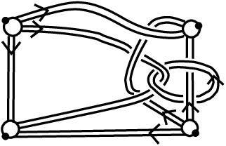
Refer to caption — Figure 1: An example of a $3$ -web

For reader’s convenience, we restate the definition of a web without invoking the notion of a ribbon graph. The role of “edges” of webs is played by bands which are embeddings of squares $[0,1]\times[0,1]$ into ${\mathbb{R}}^{3}.$ The segments $[0,1]\times\{0\}$ and $[0,1]\times\{1\}$ are the source and the target of the band, respectively. Their complement, $[0,1]\times(0,1),$ is the interior of the band.

An $n$ -web is an oriented surface embedded in ${\mathbb{R}}^{3}$ composed of a finite number of annuli, bands, and discs satisfying the following conditions:

(i)

The annuli, disks, and the interiors of the bands are disjoint from each other.
(ii)

The sources and the targets of bands are disjoint from each other and all of them lie in the boundaries of discs.
(iii)

The boundary of every disk contains either precisely $n$ sources and no targets of bands, in which case the disc is called a source, or it contains precisely $n$ targets and no sources of bands. In the that case, the disk is called a sink of the web.
(iv)

The marked boundary points of disks lie outside the sources and targets of bands.

Since each $n$ -web retracts to its spine, which is an oriented graph, often the bands and discs of webs will be called its edges and vertices, respectively. In this terminology, each vertex $v$ of a web is $n$ -valent and all edges adjacent to $v$ are either directed outwards, if $v$ is a source, or inwards, if $v$ is a sink. Notice that each web has an equal number of sources and sinks.

Our definition of $n$ -webs is modeled on the notion of $n$ -valent graphs considered in [33], cf. Section 3.2. The $n$ -webs extend the notion of webs for the geometric $A_{1}$ -spider introduced in [23], cf. Section 1.4.

By analogy with the notion of a link diagram, an $n$ -web diagram is a projection $\pi:\Gamma\to{\mathbb{R}}^{2}$ of an $n$ -web $\Gamma$ into ${\mathbb{R}}^{2}$ which is an embedding of $\Gamma$ except for a finite set of transverse (double) intersections of bands of $\Gamma$ called crossings. We require that $\pi$ preserves the orientation of $\Gamma$ (considered as an oriented surface) and that it embeds the sinks and the sources into ${\mathbb{R}}^{2}$ away from the intersections. In particular, unlike in [32], a web diagram is not allowed to have twists,

, in their bands. Each web $\Gamma$ is represented by a web diagram; for example:

$=$

1.2 The bracket isotopy invariant of $n$ -webs

For any permutation $\sigma\in S_{n},$ define the length of $\sigma$ , $l(\sigma),$ to be the minimal number of factors in the decomposition of $\sigma$ into elementary transpositions $(i,i+1),$ $i=1,...,n-1,$

l(\sigma)=\#\{(i,j):1\leq i<j\leq n,\ \sigma(i)>\sigma(j)\}.

(1)

For $\sigma\in S_{n},$ let

denote the positive braid with $l(\sigma)$ crossings representing $\sigma.$ Such braid is unique. Let $[n]=\frac{q^{n}-q^{-n}}{q-q^{-1}}$ and let $[n]!=[1]\cdot...\cdot[n].$

Theorem 1.

There exists a unique isotopy invariant of $n$ -webs, $\left\langle\Gamma\right\rangle_{n}\in{\mathbb{Z}}[q^{\pm\frac{1}{n}}],$ satisfying the following conditions:

(i)

$q^{\frac{1}{n}}\left\langle\parbox{21.68121pt}{\psfig{figure,height}}\right\rangle_{n}-q^{-\frac{1}{n}}\left\langle\parbox{21.68121pt}{\psfig{figure,height}}\right\rangle_{n}=(q-q^{-1})\left\langle\parbox{21.68121pt}{\psfig{figure,height}}\right\rangle_{n}$
(ii)

$\left\langle\parbox{21.68121pt}{\psfig{figure,height}}\right\rangle_{n}=q^{n-n^{-1}}\left\langle\parbox{14.45377pt}{\psfig{figure,height}}\right\rangle_{n},$ $\left\langle\parbox{21.68121pt}{\psfig{figure,height}}\right\rangle_{n}=q^{n^{-1}-n}\left\langle\parbox{14.45377pt}{\psfig{figure,height}}\right\rangle_{n},$
(iii)

$\left\langle\parbox{36.135pt}{\psfig{figure,height}}\hskip-7.22743pt\right\rangle_{n}\hskip-7.22743pt=q^{n(n-1)}\cdot\sum_{\sigma\in S_{n}}(-q^{\frac{1-n}{n}})^{l(\sigma)}\left\langle\parbox{36.135pt}{\psfig{figure,height}}\ \right\rangle_{n}.$
(iv)

$\left\langle\Gamma\cup\parbox{14.45377pt}{\psfig{figure,height}}\right\rangle_{n}=[n]\left\langle\Gamma\right\rangle_{n}.$ Here denotes the trivial framed knot unlinked with $\Gamma.$
(v)

$\left\langle\emptyset\right\rangle_{n}=1$ and, consequently, $\left\langle\parbox{14.45377pt}{\psfig{figure,height}}\right\rangle_{n}=[n].$

Proof.

The hard part of the statement – the existence of the bracket – follows from Theorem 17 stated in Section 2. The uniqueness of the bracket follows from the fact that each web $\Gamma$ has an equal number of sinks and sources, and, therefore, condition (iii) makes possible to represent $\left\langle\Gamma\right\rangle_{n}$ by a linear combination of brackets of framed links. On the other hand, the bracket for framed links is determined by conditions (i),(ii), (iv) and (v). ∎

Relation (iii) appeared in an implicit form in [4, 37] already.

The skein relations of Theorem 1, appear in the most natural, but not necessarily, the simplest form. If $w(\Gamma)$ denotes the writhe (ie. the sum of signs of crossings) of a web diagram $\Gamma,$ and $v(\Gamma)$ is the number of sinks of $\Gamma$ then

P_{n}(\Gamma)=q^{(n^{-1}-n)w(\Gamma)-n(n-1)v(\Gamma)}\left\langle\Gamma\right\rangle_{n}

is invariant under all Reidemeister moves. Furthermore, it satisfies the standard skein relations of the $SU(n)$ -quantum invariants, cf. [35, Thm 4.2.1]:

•

$q^{n}P_{n}\left(\parbox{21.68121pt}{\psfig{figure,height}}\right)-q^{-n}P_{n}\left(\parbox{21.68121pt}{\psfig{figure,height}}\right)=(q-q^{-1})P_{n}\left(\parbox{21.68121pt}{\psfig{figure,height}}\right),$
•

$P_{n}\left(L\cup\parbox{14.45377pt}{\psfig{figure,height}}\right)=[n]P_{n}(L).$

and the additional relation:

\bullet\ P_{n}\left(\parbox{36.135pt}{\psfig{figure,height}}\hskip-7.22743pt\right)\hskip-7.22743pt=\sum_{\sigma\in S_{n}}(-q^{n-1})^{l(\sigma)}P_{n}\left(\parbox{36.135pt}{\psfig{figure,height}}\ \right).

Proposition 2 (Proof in Section 6).

\left\langle\parbox{21.68121pt}{\psfig{figure,height}}\right\rangle_{n}=q^{\frac{n-1}{n}}\left\langle\parbox{21.68121pt}{\psfig{figure,height}}\right\rangle_{n}-q^{-\frac{n(n-1)}{2}-\frac{1}{n}}\frac{1}{[n-2]!}\left\langle\parbox{36.135pt}{\psfig{figure,height}}\right\rangle_{n},

where the band labeled by $n-2$ represents $n-2$ parallel bands.

The above relation generalizes the Kauffman bracket skein formula and it makes possible to represent any link (or web) as a linear combination of webs with no crossings. A state-sum formula for the bracket of webs with no crossings is provided in Section 1.6. Note that various renormalizations of $\left\langle\cdot\right\rangle_{n}$ are possible, leading to a skein formula of Proposition 2 without fractional coefficients. Nonetheless, our definition seems to be the most natural one, cf. Section 2, and leading to the simplest state sum formula.

The following result shows that the bracket $\left\langle\Gamma\right\rangle_{n}$ for $n$ odd does not depend on the choice of marked points on the vertices of $\Gamma.$

Proposition 3 (Proof in Section 7).

If $\Gamma,$ $\Gamma^{\prime}$ are $n$ -webs which differ by the choice of marked points on the boundaries of their discs (vertices) only, then

(i)

$\left\langle\Gamma\right\rangle_{n}=\left\langle\Gamma^{\prime}\right\rangle_{n}$ if $n$ is odd, and
(ii)

$\left\langle\Gamma\right\rangle_{n}=\left\langle\Gamma^{\prime}\right\rangle_{n}$ mod $2$ if $n$ is even.

1.3 The Kauffman bracket and $\left\langle\cdot\right\rangle_{2}$

The Kauffman bracket $[L]\in{\mathbb{Z}}[A^{\pm 1}]$ is an invariant of unoriented framed links $L\subset S^{3}$ given by the following skein conditions:

\left[\parbox{18.06749pt}{\psfig{figure,height}}\right]=A\left[\parbox{14.45377pt}{\psfig{figure,height}}\right]+A^{-1}\left[\parbox{14.45377pt}{\psfig{figure,height}}\right],\quad\left[L\cup\parbox{14.45377pt}{\psfig{figure,height}}\right]=(-A^{2}-A^{-2})[L],\quad[\emptyset]=1.

Theorem 4.

For any $2$ -web diagram $D,$

\left\langle D\right\rangle_{2}=(-1)^{w(D)+c(D)}[D],

where $A=q^{\frac{1}{2}},$ $w(D)$ denotes the sum of signs of crossings of $D$ and $c(D)$ is the number of components of the link represented by $D.$ (On the right side $D$ is considered as an unoriented framed link diagram).

Proof.

The bracket $\left\langle\cdot\right\rangle_{2}$ for links is uniquely determined by conditions (i),(ii),(iv) and (v) of Theorem 1. Since $(-1)^{w(D)+c(D)}[D]$ satisfies these relations, the statement follows. ∎

Note that the bracket of any $2$ -web $\Gamma$ can be expressed by the bracket of a framed link by the following operations:

\left\langle\parbox{21.68121pt}{\psfig{figure,height}}\right\rangle_{2}=q\left\langle\parbox{14.45377pt}{\psfig{figure,height}}\right\rangle_{2},\quad\left\langle\parbox{21.68121pt}{\psfig{figure,height}}\right\rangle_{2}=-q\left\langle\parbox{14.45377pt}{\psfig{figure,height}}\right\rangle_{2}.

These equations follow from Theorem 1. For example,

\left\langle\parbox{21.68121pt}{\psfig{figure,height}}\right\rangle_{2}=\left\langle\parbox{28.90755pt}{\psfig{figure,height}}\right\rangle_{2}=q^{2}\left(\parbox{28.90755pt}{\psfig{figure,height}}-q^{-\frac{1}{2}}\parbox{28.90755pt}{\psfig{figure,height}}\right)=

q^{2}\left(q^{-\frac{3}{2}}q^{-\frac{3}{2}}-q^{-\frac{1}{2}}q^{-\frac{3}{2}}(q+q^{-1})\right)\left\langle\parbox{14.45377pt}{\psfig{figure,height}}\right\rangle_{2}=-q\left\langle\parbox{14.45377pt}{\psfig{figure,height}}\right\rangle_{2}.

1.4 Kuperberg’s bracket and $\left\langle\cdot\right\rangle_{3}$

Kuperberg defined an invariant of framed graphs which are defined as our $3$ -webs but without marked points on their vertices, [23]. His bracket is defined by the following relations, in which we substituted his $q$ by $q^{-2}$ :

(i)

$\parbox{21.68121pt}{\psfig{figure,height}}=q^{-\frac{1}{3}}\parbox{28.90755pt}{\psfig{figure,height}}+q^{\frac{2}{3}}\parbox{21.68121pt}{\psfig{figure,height}}$
(ii)

$\parbox{21.68121pt}{\psfig{figure,height}}=q^{\frac{1}{3}}\parbox{28.90755pt}{\psfig{figure,height}}+q^{-\frac{2}{3}}\parbox{21.68121pt}{\psfig{figure,height}}$
(iii)

$\parbox{14.45377pt}{\psfig{figure,height}}=[3]$
(iv)

$\parbox{28.90755pt}{\psfig{figure,height}}=-[2]\parbox{14.45377pt}{\psfig{figure,height}}$
(v)

$\parbox{28.90755pt}{\psfig{figure,height}}=\parbox{21.68121pt}{\psfig{figure,height}}+\parbox{21.68121pt}{\psfig{figure,height}}.$

Additionally, (i) and (ii) imply

(vi)

$q^{\frac{1}{3}}\parbox{21.68121pt}{\psfig{figure,height}}-q^{-\frac{1}{3}}\parbox{21.68121pt}{\psfig{figure,height}}=(q-q^{-1})\parbox{21.68121pt}{\psfig{figure,height}}$

and (i) and (iv) imply

(vii)

$\parbox{21.68121pt}{\psfig{figure,height}}=q^{\frac{8}{3}}\parbox{14.45377pt}{\psfig{figure,height}}$ .

Theorem 5.

Kuperberg’s bracket of any web $\Gamma$ is equal to $(-q)^{-\frac{3}{2}v(\Gamma)}\left\langle\Gamma\right\rangle_{3},$ where $v(\Gamma)$ is the number of $3$ -valent vertices of $\Gamma.$ (By Theorem 3(i), $\left\langle\Gamma\right\rangle_{3}$ is well defined.)

Proof.

It is straightforward to check that $q^{-v(\Gamma)}\left\langle\Gamma\right\rangle_{3}$ satisfies relations (i),(iii), (vi), and (vii). These equations uniquely determine Kuperberg’s bracket: (i) makes possible to express Kuperberg’s bracket of every Kuperberg’s web as a linear combination Kuperberg’s brackets of framed links. These are uniquely determined by (i),(iii),(vi), and (vii). ∎

1.5 Bracket isotopy invariant of framed singular links

A singular framed link is a ribbon graph whose each vertex has two sinks and two sources. In particular, every oriented framed link is singular.

There is a map

\Psi_{n}:\{\text{singular framed links in ${\mathbb{R}}^{3}$}\}\to\{\text{$n$-webs in ${\mathbb{R}}^{3}$}\},

replacing each vertex in a singular framed link by two $n$ -valent vertices connected by $n-2$ parallel edges:

\parbox{21.68121pt}{\psfig{figure,height}}\to\parbox{36.135pt}{\psfig{figure,height}}

For any singular link diagram $D$ , let

(D)_{n}=\frac{\left\langle\Psi(D)\right\rangle_{n}}{\left([n-2]!q^{n(n-1)/2}\right)^{v(D)}}\cdot q^{w(D)/n},

where $v(D)$ is the number of singularities of $D$ (ie. $4$ -valent vertices) and $w(D)$ is the number of positive crossings minus negative crossings.

Theorem 6.

$(\Gamma)_{n}\in{\mathbb{Z}}[q^{\pm n}],$ and

(i)

$\left(\parbox{21.68121pt}{\psfig{figure,height}}\right)_{n}=q\left(\parbox{21.68121pt}{\psfig{figure,height}}\right)_{n}-\left(\parbox{21.68121pt}{\psfig{figure,height}}\right)_{n},$
(ii)

$\left(\parbox{21.68121pt}{\psfig{figure,height}}\right)_{n}=q^{-1}\left(\parbox{21.68121pt}{\psfig{figure,height}}\right)_{n}-\left(\parbox{21.68121pt}{\psfig{figure,height}}\right)_{n},$
(iii)

$\left(\parbox{21.68121pt}{\psfig{figure,height}}\right)_{n}=q^{n}\left(\parbox{21.68121pt}{\psfig{figure,height}}\right)_{n},$ $\left(\parbox{21.68121pt}{\psfig{figure,height}}\right)_{n}=q^{-n}\left(\parbox{21.68121pt}{\psfig{figure,height}}\right)_{n},$
(iv)

$\left(L\cup\parbox{14.45377pt}{\psfig{figure,height}}\right)_{n}=[n](L)_{n}.$
(v)

$\left(\emptyset\right)_{n}=1$ and, consequently, $\left(\parbox{14.45377pt}{\psfig{figure,height}}\right)_{n}=[n].$

Proof.

(i) follows from Proposition 2. (ii) follows from (i) and Theorem 1(i). Parts (iii)–(v) follow from Theorem 1(ii),(iv) and (v). ∎

$(\cdot)$ is a version of the Kauffman-Vogel bracket, [18], Furthermore, it is related to the Murakami-Ohtsuki-Yamada bracket, [27, §3] (see also [26]) in the following manner: Given a singular framed link $L,$ label all its edges by $1$ and replace each of its vertices by a pair of $3$ -valent vertices,

\parbox{21.68121pt}{\psfig{figure,height}}\to\parbox{36.135pt}{\psfig{figure,height}}.

Denote the colored ribbon graph obtained in this way by $\Phi(L).$

Proposition 7.

$(L)_{n}$ is equal to the Murakami-Ohtsuki-Yamada bracket of $\Phi(L)$ when our $q$ is identified with $q^{\frac{1}{2}}$ in [27].

Proof.

It follows from [27] that the MOY bracket of $\Phi(L)$ satisfies conditions (i)-(v) of Theorem 6. These conditions determine $(\cdot)$ uniquely. ∎

The above proposition relates the Murakami-Ohtsuki-Yamada bracket with our bracket for some graphs only. We will see in Section 1.7, that Murakami-Ohtsuki-Yamada bracket of every $3$ -valent graph with a flow is determined by our bracket of a corresponding $n$ -web.

Khovanov and Rozansky use $(\cdot)$ to define a homology theory whose extended Euler characteristic is the $SU_{n}$ -quantum invariant, [21].

1.6 State sum formula for the brackets of planar webs

An important future of Kauffman bracket is that it is given by a simple state sum formula. We describe a generalization of this formula for our bracket of $n$ -webs below. An $n$ -web diagram $\Gamma$ is planar if it has no crossings. Since Proposition 2 makes possible to express the bracket of any $n$ -web as a linear combination of brackets of planar $n$ -webs, we formulate a state sum formula planar webs only.

A state $S$ of a planar $n$ -web diagram $\Gamma$ is a labeling of its annuli and bands $e$ by numbers $S(e)\in\{1,...,n\}$ such that the bands attached to every disc are labeled by different numbers. (There is no restriction on labeling of annuli.)

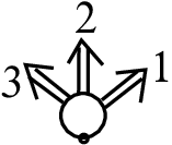
Note that every state of $\Gamma$ determines an ordering of edges adjacent to every vertex $v$ of $\Gamma.$ However, there is also a natural ordering of edges adjacent to $v,$ which does not depend on the choice of a state: If $v$ is a sink then we order the edges from $1$ to $n$ by starting at the base point of the disc $v$ and then by moving clockwise around its boundary. If $v$ is a source then we start at the base point of the disc $v$ and move counter-clockwise around its boundary.

Figure 3: The canonical ordering of bands adjacent to a sink and a source for

n=3

For any state $S$ and a vertex $v$ of $\Gamma,$ let $P(S,v)(i)$ denote the label associated by the state $S$ with the $i$ th band attached to $v.$ Hence $P(S,v)\in S_{n}.$

For any state $S,$ we define the rotation index of $S$ as follows.

rot_{n}(S)=\sum_{e}ind(a)(2S(e)-n-1),

(2)

where the sum is over all annuli and bands of $\Gamma.$ If $e$ is an annulus, then $ind(e)$ is either $+1$ or $-1$ depending on whether $e$ is oriented anti-clockwise or clockwise. The indices $ind(e)$ for edges $e$ of $\Gamma$ are defined as follows: For each band $e$ in an $n$ -web $\Gamma$ choose a smooth embedded arc

\alpha_{e}:[0,1]\to\text{the band $e$}\cup\text{the sink of $e$}\cup\text{the source of $e$}

connecting the marked points of the sink and the source.

Choose the arcs $\alpha_{e}$ such that for different bands $e,e^{\prime}$ the arcs $\alpha_{e},$ $\alpha_{e^{\prime}}$ are disjoint, except possibly meeting at one or two of their endpoints. The union $\bigcup_{e}\alpha_{e}$ taken over all bands $e$ of $\Gamma$ forms an oriented $n$ -valent graph $\Gamma^{\prime}$ in ${\mathbb{R}}^{2}.$ We say that $\Gamma^{\prime}$ is a core of $\Gamma$ if for every vertex $v$ of $\Gamma^{\prime}$ the tangent vectors at $v$ of arcs having one of their endpoints at $v$ are pointing in the same direction.

Given a core $\Gamma^{\prime}$ of $\Gamma,$ for every band $b$ in $\Gamma$ we define its winding number,

ind(b)=\frac{1}{2\pi i}\int_{0}^{1}\frac{\alpha_{b}^{\prime\prime}(t)}{\alpha_{b}^{\prime}(t)}dt,

where we identify ${\mathbb{R}}^{2}$ with ${\mathbb{C}}$ and assume that $\alpha_{b}:[0,1]\to{\mathbb{C}}.$ Note that $ind(b)=\frac{\beta}{2\pi}$ mod ${\mathbb{Z}},$ where $\beta$ is the angle between the tangent vectors to $\alpha_{b}$ at its endpoints.

Lemma 8 (Proof in Section 8).

For any state $S$ of an $n$ -web $\Gamma,$ $rot_{n}(S)$ is independent of the choice of a core of $\Gamma.$ Furthermore, $rot_{n}(S)$ is an isotopy invariant of $\Gamma$ and $rot_{n}(S)\in{\mathbb{Z}}.$

Theorem 9 (Proof in Section 8).

For any planar $n$ -web $\Gamma,$

\left\langle\Gamma\right\rangle_{n}=\sum_{S}q^{rot_{n}(S)}\prod_{v}(-q)^{l(P(S,v))},

where the sum is taken over all states of $\Gamma$ and the product is over all its vertices.

We leave the proof of the following proposition to the reader.

Proposition 10.

Let $\Gamma$ be a planar $n$ -web obtained by resolving all crossings of a link by the skein relation of Proposition 2, (In other words, let $\Gamma$ be one of the leaves of the skein tree of $L$ ). Then $\sum_{v}l(P(S,v))$ is even for any state $S$ . Consequently, all coefficients of $\left\langle\Gamma\right\rangle_{n}\in{\mathbb{Z}}[q^{\pm 1}]$ are non-negative.

1.7 Murakami-Ohtsuki-Yamada colored $3$ -valent graphs

Murakami, Ohtsuki, and Yamada defined an $SU_{n}$ -quantum invariant of links by using $3$ -valent graphs with a flow. Inspired by their work, we say that a $3$ -valent oriented, framed graph embedded into ${\mathbb{R}}^{3}$ is a Murakami-Ohtsuki-Yamada graph (MOY-graph, for short) if the edges of $\Gamma$ are labeled by positive integers forming a flow on $\Gamma:$

We allow annuli embedded into ${\mathbb{R}}^{3}$ colored by positive integers as components of MOY-graphs as well.

An MOY-graph $\Gamma$ is an $MOY_{n}$ -graph if the labels of its edges and annuli do not exceed $n.$ The purpose of this section is to show that our bracket of $n$ -webs defines a bracket invariant of $MOY_{n}$ -graphs, which coincides (up to a normalization) with the Murakami-Ohtsuki-Yamada bracket.

For any $MOY_{n}$ -graph diagram $\Gamma$ with no crossings, let $W(\Gamma)$ be a ribbon graph obtained by replacing all vertices of $\Gamma$ as follows:

\parbox{46.97505pt}{\psfig{figure,height}}\to\parbox{50.58878pt}{\psfig{figure,height}}\hskip 21.68121pt,\qquad\parbox{46.97505pt}{\psfig{figure,height}}\to\parbox{46.97505pt}{\psfig{figure,height}}

As before, an edge of a web labeled by $i$ denotes $i$ parallel edges. Let

[\Gamma]_{n}=\left\langle W(\Gamma)\right\rangle_{n}.

Corollary 11.

$[\Gamma]_{n}$ is an isotopy invariant of $MOY_{n}$ -graphs.

We are going to show that $[\Gamma]_{n}$ is a renormalization of the Murakami-Ohtsuki-Yamada bracket of $\Gamma.$

For any MOY-graph $\Gamma$ denote the labels of edges $e$ of $\Gamma$ by $|e|.$ For any vertex $v$ of $\Gamma,$ denote the adjacent edge with the largest label by $e^{v}_{0},$ and the left and the right of the two other adjacent edges by $e^{v}_{1}$ and by $e^{v}_{2}$ respectively. Hence the adjacent edges to $v$ in $\Gamma$ are either

By the definition of a flow, $|e^{v}_{0}|=|e^{v}_{1}|+|e^{v}_{2}|$ for any vertex $v.$

We say that a function $s$ assigning an $|e|$ -element subset of $\{1,...,n\}$ to every edge $e$ of $\Gamma$ is an $n$ -state (or, simply, a state) of $\Gamma$ if $s(e^{v}_{1})\cap s(e^{v}_{2})=\emptyset$ and $s(e^{v}_{1})\cup s(e^{v}_{2})=s(e^{v}_{0})$ for every vertex $v.$

Note that our definition coincides with the definition of [27] if the sets $s(e)=\{i_{1},...,i_{|e|}\}$ and $\{i_{1}-\frac{n-1}{2},i_{2}-\frac{n-1}{2},...,i_{|e|}-\frac{n-1}{2}\}$ are identified.

Any $n$ -state $s$ splits $\Gamma$ into several simple closed loops (which may intersect each other), each labeled by an integer between $1$ and $n.$ Following [27], let the rotation number of an $n$ -state $s$ be

rot(s)=\sum_{C}(s(C)-\frac{n+1}{2})rot(C)\in\frac{1}{2}{\mathbb{Z}},

where the sum is over all simple closed loops $C$ of the splitting of $\Gamma$ by $s,$ $s(C)$ is the label of $C,$ and $rot(C)$ is either $+1$ or $-1$ depending on whether $C$ is oriented anti-clockwise or clockwise.

As in [27], for any two sets $s_{1},s_{2}\subset\{1,...,n\}$ we denote by $\pi(s_{1},s_{2})$ the number of pairs $(i_{1},i_{2})\subset s_{1}\times s_{2}$ such that $i_{1}>i_{2}.$

Proposition 12 (Proof in Section 9).

For any $MOY_{n}$ -graph diagram $\Gamma$ with no crossings

[\Gamma]_{n}={\cal N}(\Gamma)\sum_{\text{$n$-states}\ s}q^{2rot(s)}\prod_{\text{vertices}\ v}(-q)^{\pi(s(e_{1}^{v}),s(e_{2}^{v}))}.

${\cal N}(\Gamma)$ is a normalization factor,

{\cal N}(\Gamma)=\prod_{e}[|e|]!\cdot\prod_{v}q^{\frac{n(n-1)-|e^{v}_{1}|\cdot|e^{v}_{2}|}{2}}[n-|e_{0}^{v}|]!

where the first product is taken over all edges of $\Gamma$ and the second product is over all vertices of $\Gamma.$ (Annuli of $\Gamma$ are not considered as edges.)

In order to avoid confusion with our bracket, we denote the $n$ -th Murakami-Ohtsuki-Yamada bracket of an $MOY_{n}$ -graph $\Gamma$ by $\{\Gamma\}_{n}.$

Proposition 13 (Proof in Section 10).

For any $MOY_{n}$ -graph diagram $\Gamma$ with no crossings,

\{\Gamma\}_{n}=q^{-\frac{1}{4}\sum_{v}|e_{1}^{v}|\cdot|e_{2}^{v}|}\sum_{\text{states}\ s}q^{rot(s)}\prod_{\text{vertices}\ v}q^{\pi(s(e_{1}^{v}),s(e_{2}^{v}))/2}.

The following lemma is needed to relate the brackets $\{\cdot\}_{n}$ and $\left\langle\cdot\right\rangle_{n}:$

Lemma + Definition 14.

For any MOY-graph $\Gamma,$

\eta_{n}(\Gamma)=2rot(s)\mod 2

does not depend on the $n$ -state $s$ of $\Gamma.$

Proof.

Since $2rot(s)=(n+1)\sum_{C}rot(C)$ mod $2,$ it is enough to show that for any state $s$ , the induced splitting of $\Gamma$ into simple loops $\{C\}$ is such that $\sum_{C}rot(C)$ does not depend on $s.$ To prove that, consider all cups and caps, $c,$ of $\Gamma.$ Each of them, being a part of an edge of $\Gamma$ , has an associated flow $|c|.$ Let $rot(c)$ be either $+1/2$ or $-1/2$ depending on whether $c$ is oriented anti-clockwise or clockwise,

\begin{array}[]{cccc}\parbox{14.45377pt}{\psfig{figure,height}}&\parbox{14.45377pt}{\psfig{figure,height}}&\parbox{14.45377pt}{\psfig{figure,height}}&\parbox{14.45377pt}{\psfig{figure,height}}\\ rot(c)=-1/2&rot(c)=1/2&rot(c)=1/2&rot(c)=-1/2\\ \end{array}

Note that

\sum_{C}rot(C)=\sum_{\text{cups and caps}:\ c}|c|rot(c),

and hence the left hand side does not depend on $s.$ ∎

By Proposition 13,

\{\Gamma\}_{n}q^{\frac{1}{4}\sum_{v}|e_{1}^{v}|\cdot|e_{2}^{v}|}\in{\mathbb{Z}}[q^{\pm\frac{1}{2}}]

and, by Proposition 12, substitution $q^{\frac{1}{2}}\to-q$ gives

\left(\{\Gamma\}_{n}q^{\frac{1}{4}\sum_{v}|e_{1}^{v}|\cdot|e_{2}^{v}|}\right)_{q^{\frac{1}{2}}\to-q}=\sum_{\text{states}\ s}q^{2rot(s)}\prod_{\text{vertices}\ v}(-q)^{\pi(s(e_{1}^{v}),s(e_{2}^{v}))}=

=[\Gamma]_{n}\cdot(-1)^{\eta_{n}(\Gamma)}/{\cal N}(\Gamma).

Corollary 15.

The value of the Murakami-Ohtsuki-Yamada bracket of any $MOY_{n}$ -graph $\Gamma$ is determined by $\left\langle W(\Gamma)\right\rangle_{n}.$

2 Definition of the bracket using tensors

We will state now another, more explicit definition of the bracket of $n$ -webs, which utilizes the construction of Reshetikhin and Turaev, [32]. Given a ribbon Hopf algebra $H,$ they constructed an isotopy invariant for ribbon graphs whose edges are labeled by representations of $H$ and whose vertices are labeled by $H$ -invariant tensors. We are going to see that our bracket $\left\langle\Gamma\right\rangle_{n}$ is the Reshetikhin-Turaev quantum $sl(n)$ invariant for $\Gamma$ considered as a ribbon graph whose edges are decorated by the defining representation $V$ and whose sinks and sources and decorated by an element of the $1$ -dimensional representation $\bigwedge^{n}V\subset V^{\otimes n}$ and by its dual, respectively.

Let $V$ be an $n$ -dimensional vector space over ${\mathbb{C}}(q)$ with a basis $e_{1},...,e_{n}.$ Given a web diagram $\Gamma$ decompose it into pieces with the following tensors associated with them:

\begin{array}[]{cccc}\parbox{21.68121pt}{\psfig{figure,height}}&\parbox{21.68121pt}{\psfig{figure,height}}&\parbox{21.68121pt}{\psfig{figure,height}}&\parbox{21.68121pt}{\psfig{figure,height}}\\ Id_{V}&Id_{V^{*}}&\hat{R}&{\hat{R}}^{-1},\\ \end{array}

(3)

where $\hat{R}:V\otimes V\to V\otimes V$ is given by

{\hat{R}}(e_{i}\otimes e_{j})=q^{-\frac{1}{n}}\begin{cases}e_{j}\otimes e_{i}&\text{if $i>j$,}\\ qe_{i}\otimes e_{j}&\text{if $i=j$,}\\ e_{j}\otimes e_{i}+(q-q^{-1})e_{i}\otimes e_{j}&\text{if $i<j$.}\\ \end{cases}

(4)

\begin{array}[]{cccc}\parbox{14.45377pt}{\psfig{figure,height}}&\parbox{14.45377pt}{\psfig{figure,height}}&\parbox{14.45377pt}{\psfig{figure,height}}&\parbox{14.45377pt}{\psfig{figure,height}}\\ \text{\small$\sum_{i}e^{i}\otimes e_{j}\to\delta_{ij}$}&\text{\small$e_{i}\otimes e^{j}\to q^{2i-n-1}\delta_{ij}$}&\text{\small$1\to\sum_{i}e_{i}\otimes e^{i}$}&\text{\small$1\to\sum_{i}q^{n+1-2i}e^{i}\otimes e_{i}$}\\ \text{\small$V^{*}\otimes V\to{\mathbb{C}}(q)$}&\text{\small$V\otimes V^{*}\to{\mathbb{C}}(q)$}&\text{\small${\mathbb{C}}(q)\to V\otimes V^{*}$}&\text{\small${\mathbb{C}}(q)\to V^{*}\otimes V$}\\ \end{array}

(5)

\begin{array}[]{cc}\parbox{21.68121pt}{\psfig{figure,height}}&\parbox{21.68121pt}{\psfig{figure,height}}\\ \text{\small${\cal T}_{-}:V^{\otimes n}\to{\mathbb{C}}(q)$}&\text{\small${\cal T}_{+}:{\mathbb{C}}(q)\to V^{\otimes n}$,}\\ \end{array}

(6)

where

{\cal T}_{+}(1)=T_{+}=\sum_{\sigma\in S_{n}}(-q)^{l(\sigma)}e_{\sigma(1)}\otimes e_{\sigma(2)}\otimes...\otimes e_{\sigma(n)},

(7)

and

{\cal T}_{-}(e_{i_{1}}\otimes...\otimes e_{i_{n}})=\begin{cases}(-q)^{l(\sigma)}&\text{if $(1,...,n)\to(i_{1},...,i_{n})$ is a permutation $\sigma$}\\ 0&\text{otherwise.}\\ \end{cases}

(8)

Definition 16.

For any $n$ -web diagram $\Gamma$ decomposed into pieces as above, let $\left\langle\Gamma\right\rangle_{n}\in{\mathbb{Q}}(q^{\frac{1}{n}})$ be the scalar obtained by the contraction of the corresponding tensors.

Theorem 17 (Proof in Section 5).

(i)

The bracket defined above is an isotopy invariant of $n$ -webs.
(ii)

It satisfies the properties of the bracket stated in Theorem 1.

Consequently, Definition 16 coincides with the definition of the bracket given in Theorem 1.

3 The $SU(n)$ -skein modules of $3$ -manifolds

3.1 The definition of the skein module

Let $M$ be an orientable $3$ -manifold, possibly with non-empty boundary, and let $n\geq 2.$ Let ${\cal W}_{n}(M)$ denote the set of all isotopy classes of $n$ -webs embedded into $M,$ including the empty web, $\emptyset.$ Consider a ring $R$ with a specified invertible element $t.$ The $SU(n)$ -skein module of $M$ with coefficients in $R$ is the quotient of the free $R$ -module $R{\cal W}_{n}(M)$ by relations

(i)

$t\parbox{21.68121pt}{\psfig{figure,height}}-t^{-1}\parbox{21.68121pt}{\psfig{figure,height}}-(t^{n}-t^{-n})\parbox{21.68121pt}{\psfig{figure,height}}$
(ii)

$\parbox{21.68121pt}{\psfig{figure,height}}-t^{n^{2}-1}\parbox{14.45377pt}{\psfig{figure,height}},$ $\parbox{21.68121pt}{\psfig{figure,height}}-t^{1-n^{2}}\parbox{14.45377pt}{\psfig{figure,height}},$
(iii)

$\parbox{36.135pt}{\psfig{figure,height}}\hskip-7.22743pt\hskip-7.22743pt-t^{n^{3}-n^{2}}\cdot\sum_{\sigma\in S_{n}}(-t^{(1-n)})^{l(\sigma)}\parbox{36.135pt}{\psfig{figure,height}}.$
(iv)

$\Gamma\cup\parbox{14.45377pt}{\psfig{figure,height}}-[n]\Gamma.$

Note that the above relations correspond to equations (i)-(v) of Theorem 1, after the substitution $t=q^{\frac{1}{n}}.$ We denote the quotient module by ${\cal S}_{n}(M;R,t).$

The $SU_{3}$ -skein module was defined independently in [8], and earlier, for $3$ -dimensional thickenings of surfaces, in [28]. The definitions of Frohman-Zhong and Ohtsuki-Yamada are equivalent to ours, since their skein relations are the skein relations for $q^{-v(\Gamma)}\left\langle\Gamma\right\rangle_{n},$ when $A=-q^{\frac{1}{3}}=-t,$ cf. Theorem 5.

Theorem 4 implies the following:

Corollary 18.

${\cal S}_{2}(M;R,t)$ is isomorphic to the Kauffman bracket skein module of $M$ with coefficients in $R$ and $A=t.$

It follows directly from the definition, that if $f:R\to R^{\prime}$ is a homomorphism of rings such that $f(t)=t^{\prime}$ then

{\cal S}_{n}(M;R^{\prime},t^{\prime})={\cal S}_{n}(M;R,t)\otimes_{R}R^{\prime}.

Since for any ring $R$ with an invertible element $t$ there is a map $f:{\mathbb{Z}}[t^{\pm 1}]\to R,$ Theorem 1 can be restated as follows:

Corollary 19.

For any ring $R$ with an invertible element $t,$ ${\cal S}_{n}({\mathbb{R}}^{3};R,t)=R$

Below, we describe the relation between ${\cal S}_{n}(M;R,t)$ and $SL_{n}(R)$ -representations of $\pi_{1}(M),$ which generalizes the theorems of Bullock, [5], and ours with J. Przytycki, [30], for the Kauffman bracket skein modules. Further analysis of $SU(n)$ -skein modules is postponed to [34]. The discussion below and the results of [34] show that $SU(n)$ -skein modules have many properties analogous to those of of the Kauffman bracket skein module.

3.2 $SU(n)$ -skein modules and character varieties

Since the skein relation (i) above reduces to $\parbox{21.68121pt}{\psfig{figure,height}}=\parbox{21.68121pt}{\psfig{figure,height}}$ for $t=1,$ the $n$ -webs in $M$ , which are freely homotopic to each other, are identified in ${\cal S}_{n}(M;R,1).$ Consequently, the operation of taking the disjoint union, $\Gamma_{1},\Gamma_{2}\to\Gamma_{1}\cup\Gamma_{2},$ extends to a well defined product in ${\cal S}_{n}(M;R,1)$ making this module a commutative $R$ -algebra.

Furthermore, note that as an $R$ -algebra, ${\cal S}_{n}(M;R,1)$ is isomorphic to ${\mathbb{A}}_{n}(M)$ (over the ring of coefficients $R$ ) defined in [33]. Hence, by [33, Theorem 3.7] we have:

Corollary 20.

If ${\mathbb{K}}$ is an algebraically closed field of characteristic $0$ then ${\cal S}_{n}(M;{\mathbb{K}},1)\simeq{\mathcal{O}}(X_{n}(\pi_{1}(M))),$ where ${\mathcal{O}}(X(M))$ denotes the ring of global sections (the coordinate ring) of the $SL_{n}({\mathbb{K}})$ -character variety of $\pi_{1}(M).$

The $SL_{n}({\mathbb{K}})$ -character variety, $X_{n}(G),$ of a group $G$ is an affine algebraic scheme over ${\mathbb{K}}$ “describing” the $SL_{n}({\mathbb{K}})$ -representations of $G$ up to conjugation. More precisely, the closed points of $X_{n}(G)$ (ie. the maximal ideals in ${\mathcal{O}}(X(G))$ correspond to the semi-simple $SL_{n}({\mathbb{K}})$ -representations of $G$ up to conjugation. For a precise definition of $SL_{n}$ -character varieties see [33, 25].

Up to nilpotent elements, the ring ${\mathcal{O}}(X(G))$ can be described as follows: A characteristic function $f:SL_{n}({\mathbb{K}})\to{\mathbb{K}}$ is any polynomial in the entries of the matrices in $SL_{n}({\mathbb{K}})$ which is invariant under the conjugation by $SL_{n}({\mathbb{K}}).$ Characteristic functions of $SL_{n}({\mathbb{K}})$ form a ${\mathbb{K}}$ -algebra generated by the functions $f_{n}(A)=tr(A^{n}).$ Let $X^{\prime}(G)$ be the set of all generalized $SL_{n}$ -characters of $G,$ that is ${\mathbb{K}}$ -valued functions on $G$ of the form $\psi=f\circ\rho,$ where $\rho:G\to SL_{n}({\mathbb{K}})$ is a representation and $f$ is a characteristic function on $SL_{n}({\mathbb{K}}).$ With any $g\in G$ there is the associated “evaluation at $g$ ” function $\tau_{g}:X^{\prime}(G)\to{\mathbb{K}},$ $\tau_{g}(\psi)=\psi(g).$ The ${\mathbb{K}}$ -algebra ${\mathcal{O}}(X(G))/\sqrt{0}$ is isomorphic to the ${\mathbb{K}}$ -algebra generated by all $\tau_{g}$ for all $g.$ If we think of the functions $\tau_{g}$ as regular functions on $X_{n}^{\prime}(G),$ then for any finitely generated group $G,$ $X_{n}^{\prime}(G)$ becomes an affine algebraic set whose coordinate ring is isomorphic to ${\mathcal{O}}(X(G))/\sqrt{0}.$

4 Preliminaries for the proofs

4.1 The quantum $sl_{n}$ group and its defining representation

Let $U_{h}=U_{h}(sl_{n})$ be defined as in [22, Sect. 6.1.3]. Note that Reshetikhin’s and Turaev’s definition of $U_{h}(sl_{n}),$ [32, Sect. 7.1], coincides with our definition of $U_{h}$ after taking into account the following changes:

•

$X^{+}_{i}$ and $X^{-}_{i}$ in [32] are $E_{i}$ and $F_{i}$ in [22],
•

$h$ used by Reshetikhin and Turaev is equal to $2h$ in [22].

In this paper we will use Klimyk-Schmüdgen $h$ only. Let $V={\mathbb{C}}[[h]]^{n}$ be the defining representation of $U_{h},$ presented explicitly in [22, Sect. 8.4.1]. Additionally, consider the quantum group $U_{q}=U_{q}(sl_{n}),$ [22, Sect. 6.1.2], and its defining representation, $V=C(q)^{n},$ as defined in [22, Sect. 8.4.1]. This double meaning of $V$ will not lead to confusion since the $U_{q}$ and $U_{h}$ actions on $V$ agree if $q$ and $K_{i}$ are identified with $e^{h}$ and $e^{hH_{i}}$ respectively. In both cases, $e_{1},...,e_{n}$ will be the weight basis of $V$ with the heighest weight vector $e_{1}$ , see [22, Sect. 8.4.1].

The defining representation $\rho:U_{q}\to End(V)$ is given by the matrices

\rho(K_{i})=q^{-1}E_{ii}+qE_{i+1,i+1}+\sum_{j\neq i,i+1}E_{jj},\quad i=1,2,...,n-1,

(9)

\rho(E_{i})=E_{i+1,i},\quad\rho(F_{i})=E_{i,i+1},\quad i=1,2,...,n-1,

(10)

where $E_{ij}$ denotes the matrix whose all entries are $0$ except for the $(i,j)$ th entry which is $1,$ cf. [22, Sect. 8.4.1].

4.2 The Hecke algebra associated with $U_{q}$

For the purpose of studying $U_{q}(sl_{n})$ -actions on $V^{\otimes k}$ we define the Hecke algebra, $H_{k},$ as follows. Let $H_{k}$ be the non-commutative, associative algebra over ${\mathbb{C}}(t)$ generated by elements $g_{1}^{\pm 1},...,g_{k}^{\pm 1}$ subject to the following relations: $g_{i}g_{j}=g_{j}g_{i}$ for $|i-j|\geq 2,$ $g_{i}g_{i+1}g_{i}=g_{i+1}g_{i}g_{i+1},$ for $i=1,...,k-1,$ and $(g_{i}-t^{n})(g_{i}+t^{-n})=0$ for all $i.$ The algebra $H_{k}$ is an $k!$ -dimensional space with basis vectors $h_{\sigma},$ for $\sigma\in S_{k},$ which satisfy the following multiplication rules

(i)

$(h_{(i,i+1)}-t^{n-1})(h_{(i,i+1)}+t^{-n-1})=0$ for $i=1,...,n-1,$
(ii)

$h_{\sigma}h_{\tau}=h_{\sigma\tau}$ if $l(\sigma\tau)=l(\sigma)+l(\tau).$

We have $g_{i}=t\cdot h_{(i,i+1)}.$ Although various definitions of Hecke algebra appear in the literature, see for example [22, Sect. 8.6.4], [7, Sect. 12.3], [14], they are all isomorphic to our $H_{k}$ after a proper extension of base field. In fact, substituting the quadratic equation (i) above by any other quadratic equation with distinct roots leads an isomorphic algebra, after a finite extension of the base field. For example, Gyoja’s $q$ in [14] is our $t^{2n}$ and Gyoja’s $h(\sigma)$ is ours $t^{(n+1)l(\sigma)}h_{\sigma}.$ Our somewhat cumbersome notation is chosen so that $h_{(i,i+1)}$ ’s satisfy the same quadratic equation as $\hat{R}$ for $q=t^{n}.$ Therefore, from now on, we will assume that $q=t^{n}.$ We summarize the basic relations between $H_{n}$ and the defining representation $V$ of $U_{q}:$

Proposition 21.

(i)

$H_{k}$ acts on $V^{\otimes k}$ in such a way that the actions of $h_{\sigma}$ and of

on $V^{\otimes k}$ coincide.
(ii)

The $H_{k}$ and $U_{q}$ actions on $V^{\otimes k}$ commute.
(iii)

(Frobenius-Schur duality)\quaThe images of the maps $U_{q}\to End(V^{\otimes k})$ and $H_{n}\to End(V^{\otimes k})$ are centralizers of each other. In particular, any $U_{q}$ -equivariant endomorphism of $V^{\otimes k}$ is of the form $w\to x\cdot w$ for a certain $x\in H_{k}.$

In [14, page 843], Gyoja defines two elements $e_{+},e_{-}$ which in our notation are:

e_{+}=\sum_{\sigma\in S_{k}}q^{\frac{n+1}{n}l(\sigma)}h_{\sigma},\quad\text{and}\quad e_{-}=\sum_{\sigma\in S_{k}}(-q^{\frac{1-n}{n}})^{l(\sigma)}h_{\sigma},

(11)

and shows that

h_{\sigma}e_{+}=e_{+}h_{\sigma}=q^{\frac{n-1}{n}l(\sigma)}e_{+}\quad\text{and}\quad h_{\sigma}e_{-}=e_{-}h_{\sigma}=(-q^{-\frac{n+1}{n}})^{l(\sigma)}e_{-},

(12)

for any $\sigma\in S_{k}.$ Furthermore, for $P_{\pm}=\sum_{\sigma\in S_{k}}q^{\pm 2l(\sigma)},$ $e_{\pm}/P_{\pm}$ are primitive idempotents of $H_{k}$ : $e_{+}/P_{+}$ is the symmetrizer and $e_{-}/P_{-}$ is the antisymmetrizer.

5 Proof of Theorem 17

The isotopy invariance of the $n$ -bracket follows from [32, Theorem 5.1] and from the following proposition.

Proposition 22.

(i)

The tensors (5.1.1)-(5.1.3) in [32] for the defining $U_{h}$ -representation are given by our formulas (3)-(5). (Recall that $q=e^{\frac{h_{RT}}{2}},$ where $h_{RT}$ is the Reshetikhin-Turaev $h.$ )
(ii)

The map (7), ${\cal T}_{+}:{\mathbb{C}}(q)\to V^{\otimes n},$ is $U_{q}$ -equivariant.
(iii)

The map (8), ${\cal T}_{-}:(V^{*})^{\otimes n}\to{\mathbb{C}}(q),$ is $U_{q}$ -equivariant.

Proof of Proposition 22(i)\quaBy [22], the $R$ -matrix acts on $V\otimes V$ by the matrix

q^{-\frac{1}{n}}\left(q\sum_{i}(E_{ii}\otimes E_{ii})+\sum_{i\neq j}(E_{ii}\otimes E_{jj})+(q-q^{-1})\sum_{i>j}(E_{ij}\otimes E_{ji})\right).

(13)

(This matrix is denoted by $R_{1,1}$ in [22], cf. the first paragraph of Section 8.4.2 and (60) in [22].) Here, as before, $E_{ij}$ represents the map $\delta^{j}_{i}:V\to V,$ $\delta^{j}_{i}(e_{k})=\delta_{j,k}e_{i}.$ By composing the map represented by (13) with the transposition $\tau:V\otimes V\to V\otimes V,$ $\tau(v_{1},v_{2})=(v_{2},v_{1}),$ we obtain the map $\hat{R}$ given by (4).

The “cap” maps in [32, (5.1.1-2)] are given by the contraction map $V^{*}\otimes V\to{\mathbb{C}}[[h]],$ $(x,y)=x(y)$ and the map $V\otimes V^{*}\to{\mathbb{C}}[[h]],$ $(y,x)\to x(v^{-1}uy).$ The “cup” maps are their duals. Let us recall the meaning of $v^{-1}u$ in [32]: Let $\rho$ be the half-sum $\frac{1}{2}\sum_{\alpha\in\Delta_{+}}\alpha$ of primitive roots of $sl_{n}$ and let $\rho_{i}\in{\mathbb{Z}}$ be the coordinates of $\rho$ in the basis of the Cartan subalgebra of $sl_{n}$ given by simple roots $\alpha_{1},...,\alpha_{n-1}.$ By [32, (7.1.1)], $v^{-1}u=exp(2h\sum_{i=1}^{n-1}\rho_{i}H_{i}).$ (Recall that Reshetikhin-Turaev $h$ is twice the $h$ we use.) Therefore the following lemma completes the proof of Proposition 22(i).

Lemma 23.

$v^{-1}u$ acts on $V$ by sending $e_{k}$ to $q^{2k-n-1}e_{k}$

Proof.

Positive roots in the Cartan subalgebra of $sl_{n}$ are of the form $\alpha_{ij}=\alpha_{i}+\alpha_{i+1}+...+\alpha_{j},$ for $1\leq i\leq j\leq n-1.$ Therefore, $\alpha_{k}$ appears $\frac{1}{2}k(n-k)$ times in $\rho$ and $\rho_{k}=\frac{1}{2}k(n-k).$

By [22, Section 8.4.1], $H_{i}e_{k}$ is $-e_{k}$ if $i=k,$ $e_{k}$ if $i=k-1,$ and $0$ otherwise. Therefore,

exp(hH_{i})e_{k}=\begin{cases}q^{-1}e_{k}&\text{if i=k}\\ qe_{k}&\text{if i=k-1}\\ e_{k}&\text{otherwise}.\end{cases}

Consequently, $(v^{-1}u)e_{k}=q^{-2\rho_{k}+2\rho_{k-1}}e_{k}=q^{(k-1)(n-k+1)-k(n-k)}e_{k}=q^{2k-n-1}e_{k}.$ ∎

Proof of Proposition 22(ii) – $U_{q}$ -equivariance of ${\cal T}_{+}$

$U_{q}$ acts on the $n$ -th power of the defining representation $V,$ via the map

U_{q}\stackrel{{\scriptstyle\Delta^{n-1}}}{{\longrightarrow}}U_{q}^{\otimes n}\stackrel{{\scriptstyle\rho^{\otimes n}}}{{\longrightarrow}}End(V^{\otimes n}),

where $\Delta^{n-1}:U_{q}\to U_{q}^{n}$ is the $(n-1)$ st power of the comultiplication in $U_{q}.$ The following explicit formulas for $\Delta^{n-1}$ follow by induction on $n$ from the definition of $\Delta,$ [22, Prop 6.1.2.5]:

	$\displaystyle\Delta^{n-1}(K_{i})=K_{i}\otimes...\otimes K_{i},\text{for $i=1,...,n-1,$}$		(14)
	$\displaystyle\Delta^{n-1}(E_{i})=\sum_{j=1}^{n}1\otimes...\otimes 1\otimes\stackrel{{\scriptstyle j}}{{E_{i}}}\otimes K_{i}\otimes...\otimes K_{i},\text{for $i=1,...,n-1,$}$		(15)

where the index $j$ over $E_{i}$ means that it takes the $j$ -th position in the tensor product. For $\Delta^{n-1}(F_{i})$ we have a similar expression:

\Delta^{n-1}(F_{i})=\sum_{j=1}^{n}K_{i}^{-1}\otimes...\otimes K_{i}^{-1}\otimes\stackrel{{\scriptstyle j}}{{F_{i}}}\otimes 1\otimes...\otimes 1.

(16)

Since $U_{q}$ acts on ${\mathbb{C}}(q)$ by counit map, $\epsilon:U_{q}\to{\mathbb{C}}(q),$ which sends $E_{i},F_{i}$ to $0$ and $K_{i}$ to $1,$ we need to show that $\Delta^{n-1}(K_{i})T_{+}=T_{+},$ and $\Delta^{n-1}(E_{i})T_{+}=\Delta^{n-1}(F_{i})T_{+}=0$ for $i=1,...,n-1.$ In order to prove the first equality notice that by (9) and (14) $\Delta^{n-1}(K_{i})$ multiplies the $e_{i}$ component in $e_{\sigma(1)}\otimes...\otimes e_{\sigma(n)}$ by $q^{-1}$ and it multiplies the $e_{i+1}$ component by $q.$ Since it leaves all other components unchanged, $\Delta^{n-1}(K_{i})\cdot e_{\sigma(1)}\otimes...\otimes e_{\sigma(n)}=e_{\sigma(1)}\otimes...\otimes e_{\sigma(n)}$ and, consequently, $\Delta^{n-1}(K_{i})T_{+}=T_{+}.$ We complete the proof by showing that $\Delta^{n-1}(E_{i})T_{+}=0.$ The proof of $\Delta^{n-1}(F_{i})T_{+}=0$ is analogous and left to the reader.

For simplicity, denote $e_{\sigma(1)}\otimes...\otimes e_{\sigma(n)}\in V^{\otimes n}$ by $e_{\sigma}.$ By (1),

l((i,i+1)\sigma)=\begin{cases}l(\sigma)+1&\text{if $\sigma^{-1}(i)<\sigma^{-1}(i+1)$}\\ l(\sigma)-1&\text{otherwise.}\end{cases}

Therefore,

T_{+}=\sum_{\sigma\in S_{n}\atop\sigma^{-1}(i)<\sigma^{-1}(i+1)}(-q)^{l(\sigma)}(e_{\sigma}-qe_{(i,i+1)\sigma}),

and our goal is to prove that

\Delta^{n-1}(E_{i})\cdot(e_{\sigma}-qe_{(i,i+1)\sigma})=0,

(17)

for $\sigma$ such that $\sigma^{-1}(i)<\sigma^{-1}(i+1).$ We have

1\otimes...\otimes 1\otimes\stackrel{{\scriptstyle j}}{{E_{i}}}\otimes K_{i}...\otimes K_{i}\cdot e_{\sigma}=

\begin{cases}0&\text{if $\sigma(j)\neq i$}\\ e_{\sigma(1)}\otimes...\otimes e_{\sigma(j-1)}\otimes\stackrel{{\scriptstyle j}}{{e_{i+1}}}\otimes e_{\sigma(j+1)}\otimes...\otimes e_{\sigma(n)}&\text{if $\sigma(j)=i$ and $\sigma^{-1}(i+1)<j$}\\ qe_{\sigma(1)}\otimes...\otimes e_{\sigma(j-1)}\otimes\stackrel{{\scriptstyle j}}{{e_{i+1}}}\otimes e_{\sigma(j+1)}\otimes...\otimes e_{\sigma(n)}&\text{if $\sigma(j)=i$ and $\sigma^{-1}(i+1)>j.$}\\ \end{cases}

Therefore, if $\sigma^{-1}(i)=j$ then $\Delta^{n-1}(E_{i})\cdot e_{\sigma}=$

e_{\sigma(1)}\otimes...\otimes e_{\sigma(j-1)}\otimes\stackrel{{\scriptstyle j}}{{e_{i+1}}}\otimes e_{\sigma(j+1)}\otimes...\otimes e_{\sigma(n)}\begin{cases}q&\text{if $\sigma^{-1}(i)<\sigma^{-1}(i+1)$}\\ 1&\text{otherwise.}\\ \end{cases}

This implies (17) and, therefore, completes the proof of $U_{q}$ -equivariance of ${\cal T}_{+}.$

Proof of Proposition 22(iii) – $U_{q}$ -equivariance of ${\cal T}_{-}$

We need to prove that for any $x\in U_{q}$ and any $w=v_{j_{1}}\otimes...\otimes v_{j_{n}}\in V^{\otimes n},$ $\epsilon(x){\cal T}_{-}(w)={\cal T}_{-}(\Delta^{n-1}(x)\cdot w).$ This equality reduces to the following three sets of equations for $i=1,...,n-1:$

	$\displaystyle{\cal T}_{-}(\Delta^{n-1}(K_{i})\cdot w)={\cal T}_{-}(w)$		(18)
	$\displaystyle{\cal T}_{-}(\Delta^{n-1}(E_{i})\cdot w)=0$		(19)
	$\displaystyle{\cal T}_{-}(\Delta^{n-1}(F_{i})\cdot w)=0.$		(20)

Both sides of (18) vanish if the numbers $(i_{1},...,i_{n})$ are not distinct. On the other hand, if these numbers are distinct then $\Delta^{n-1}(K_{i})\cdot w=w$ and (18) follows. We will complete the proof by showing (19) – the proof of (20) is analogous.

Observe that $\Delta^{n-1}(E_{i})\cdot v_{j_{1}}\otimes...\otimes v_{j_{n}}$ is a linear combination of terms $v_{k_{1}}\otimes...\otimes v_{k_{n}}$ such that the $n$ -tuple $(k_{1},...,k_{n})$ is obtained from $(j_{1},...,j_{n})$ by changing one of the indices from $i$ to $i+1.$ Since ${\cal T}_{-}(v_{k_{1}}\otimes...\otimes v_{k_{n}})=0$ if the numbers $k_{1},...,k_{n}$ are not a permutation of $1,...,n,$ the left side of (19) vanishes unless $j_{1},...,j_{l-1},j_{l}+1,j_{l+1},...,j_{n}$ are a permutation $\sigma$ of $1,...,n,$ for some $l$ such that $j_{l}=i.$ In this case $j_{k}=i$ for some $k\neq l$ and we can assume that $k<l.$ Under above assumptions,

	$\displaystyle\Delta^{n-1}(E_{i})\cdot(v_{j_{1}}\otimes...\otimes v_{j_{n}})$	$\displaystyle=$	$\displaystyle v_{j_{1}}\otimes...\otimes\stackrel{{\scriptstyle k}}{{v_{i+1}}}\otimes...\otimes\stackrel{{\scriptstyle l}}{{q^{-1}v_{i}}}\otimes...\otimes v_{j_{n}}+$
			$\displaystyle v_{j_{1}}\otimes...\otimes\stackrel{{\scriptstyle k}}{{v_{i}}}\otimes...\otimes\stackrel{{\scriptstyle l}}{{v_{i+1}}}\otimes...\otimes v_{j_{n}}.$

Hence, ${\cal T}_{-}\left(\Delta^{n-1}(E_{i})\cdot(v_{j_{1}}\otimes...\otimes v_{j_{n}})\right)=(-q)^{l((i,i+1)\sigma)}\cdot q^{-1}+(-q)^{l(\sigma)}.$ Since $l((i,i+1)\sigma)=l(\sigma)+1,$ the left hand side of (19) vanishes and the proof of Proposition 22(iii) is completed.

Proof of Theorem 17(ii)\quaIn the previous section, we proved that $\left\langle\cdot\right\rangle_{n}$ is an isotopy invariant of $n$ -webs. Now we are going to show that it satisfies properties (i)-(v) formulated in Theorem 1.

(i)\quaSince Klimyk’s and Schmüdgen’s $\hat{R}$ is our $q^{\frac{1}{n}}\hat{R},$ our $\hat{R}$ satisfies

(q^{\frac{1}{n}}\hat{R}-q)(q^{\frac{1}{n}}\hat{R}+q^{-1})=0

by [22, Proposition 8.4.24] and, hence,

q^{\frac{1}{n}}\hat{R}-q^{-\frac{1}{n}}{\hat{R}}^{-1}=(q-q^{-1})I.

This implies the skein relation (i) of Theorem 1.

(ii)\quaSince the two relations (ii) of Theorem 1 are inverses of each other, we will show the first of them only.

The “kink,”

, defines a map on $V$ which is $U_{q}$ -equivariant. Since $V$ is an irreducible module, this map is a multiple of $Id_{V}$ and, therefore, for our purpose it is enough to show that the kink maps $e_{i}$ to $q^{n-\frac{1}{n}}e_{i}$ for some (and hence for arbitrary) $i.$ Choose $i=n.$ Since the arc

maps $V$ to itself by sending $e_{i}$ to $q^{2i-n-1}e_{i},$ the kink maps $e_{n}$ to $Ce_{n},$ where $C=\sum_{k=1}^{n}{\hat{r}}_{nk}^{nk}q^{2k-n-1}$ and ${\hat{r}}_{ij}^{nk}$ are the coefficients of the $\hat{R}$ -matrix,

{\hat{R}}(e_{n}\otimes e_{k})=\sum_{i,j}{\hat{r}}_{ij}^{nk}e_{i}\otimes e_{j}.

Since ${\hat{r}}^{nk}_{nk}=\begin{cases}q^{-\frac{1}{n}+1}&\text{for $k=n$}\\ 0&\text{otherwise,}\\ \end{cases}$ $C=q^{n-\frac{1}{n}}.$

(iii)\quaThis property will be proved in the next section.

(iv)\quaThe bracket of the trivial knot diagram is given by the contraction of the cup and the cap tensors, where the cup and the cap are chosen with coinciding orientations. Therefore

\left\langle\parbox{14.45377pt}{\psfig{figure,height}}\right\rangle_{n}=\sum_{i=1}^{n}q^{2i-n-1}=[n].

By the construction of the bracket, $\left\langle\Gamma_{1}\cup\Gamma_{2}\right\rangle_{n}=\left\langle\Gamma_{1}\right\rangle_{n}\cdot\left\langle\Gamma_{2}\right\rangle_{n},$ for disjoint (and hence unlinked) web diagrams $\Gamma_{1},\Gamma_{2}.$

(v)\quaThis is obvious.

6 Proof of Proposition 2 and of Theorem 1(iii)

We will often use the following equality

\sum_{\sigma\in S_{n}}(-q)^{2l(\sigma)}=q^{\frac{n(n-1)}{2}}\cdot[n]!

(21)

following from [14, (3.1)].

Lemma 24.

$\left\langle\parbox{43.36243pt}{\psfig{figure,height}}\right\rangle_{n}=q^{\frac{n(n-1)}{2}}\cdot[n]!$

Proof.

The above bracket is given by the contraction of ${\cal T}_{-}$ with ${\cal T}_{+},$

{\cal T}_{-}(T_{+})=\sum_{\sigma\in S_{n}}(-q)^{2l(\sigma)}=q^{\frac{n(n-1)}{2}}\cdot[n]!,

by (21). ∎

Consider the skein

\Lambda_{k}=\sum_{\sigma\in S_{k}}(-q^{\frac{1-n}{n}})^{l(\sigma)}\parbox{28.90755pt}{\psfig{figure,height}},

(22)

where, as before,

is the unique positive braid with $l(\sigma)$ crossings representing $\sigma.$ Given an $(k,k)$ -tangle $T,$

, denote by $\pi_{k}(T)$ the $(k-1,k-1)$ -tangle obtained from $T$ by closing up its last string,

. The definition of $\pi_{k}(T)$ obviously extends to all skeins $T$ being linear combinations of $(k,k)$ -tangles.

Lemma 25.

$\pi_{k+1}(\Lambda_{k+1})=\Lambda_{k}q^{-k}[n-k].$

Proof.

Each permutation $\sigma\in S_{k+1}$ can be written in the form

(i_{1},i_{1}-1,...,i_{1}-j_{1})(i_{2},i_{2}-1,...,i_{2}-j_{2})...(i_{l},i_{l}-1,...,i_{l}-j_{l}),

(23)

where $i_{1}<i_{2}<...<i_{l}.$ Furthermore, such presentation is unique. (These statements can be proved by induction on $k$ .) By splitting the set of all permutations $\sigma\in S_{k+1}$ into those with $i_{l}\leq k$ and those with $i_{l}=k+1,$ we get

\pi_{k+1}(\Lambda_{k+1})=\Lambda_{k}[n]+\sum_{i=1}^{k}(-q^{\frac{1-n}{n}})^{k+1-i}\parbox{57.81621pt}{\psfig{figure,height}}.

The $i$ -th summand in the sum on the right side takes into account all permutations $\sigma\in S_{k+1}$ with $i_{l}=k+1$ and $j_{l}=i.$ Note that the action of $\Lambda_{k}$ on $V^{\otimes k}$ coincides with the one of $e_{-},$ defined in (11), and hence composing $\Lambda_{k}$ with a single positive crossing on two adjacent strings yields $-q^{-\frac{n+1}{n}}\Lambda_{k}.$ Therefore, after applying relation (ii) of Theorem 1 to remove the kink in the skein above and after replacing the $k-i$ crossings by the factor $(-q^{-\frac{n+1}{n}})^{k-i}$ we get

\pi_{k+1}(\Lambda_{k+1})=\Lambda_{k}[n]+\sum_{i=1}^{k}(-q^{\frac{1-n}{n}})^{k+1-i}(-q^{-\frac{n+1}{n}})^{k-i}q^{n-n^{-1}}\Lambda_{k}=

\Lambda_{k}[n]+\Lambda_{k}q^{n-n^{-1}}(-q^{\frac{1-n}{n}})\sum_{i=1}^{k}q^{-2(k-i)}=\Lambda_{k}[n]+\Lambda_{k}(-q^{n-1})\frac{1-q^{-2k}}{1-q^{-2}}=

\Lambda_{k}\left([n]-\frac{q^{n}-q^{n-2k}}{q-q^{-1}}\right)=\Lambda_{k}\left(\frac{q^{n-2k}-q^{-n}}{q-q^{-1}}\right)=\Lambda_{k}q^{-k}[n-k].

∎

Recall that $T_{+}\in V^{\otimes n}$ was defined in (7) and $h_{i,i+1}$ in Section 4.2.

Corollary 26.

\sum_{\sigma\in S_{n}}(-q^{\frac{1-n}{n}})^{l(\sigma)}\left\langle\parbox{50.58878pt}{\psfig{figure,height}}\right\rangle_{n}=q^{-\frac{n(n-1)}{2}}[n]!

Lemma 27.

$h_{(i,i+1)}T_{+}=(-q^{-\frac{n+1}{n}})T_{+}.$

Proof.

Denote $e_{\sigma(1)}\otimes...e_{\sigma(n)}\in V^{\otimes n}$ by $e_{\sigma}$ as before. By Proposition 21(1) and (4),

h_{(i,i+1)}e_{\sigma}=q^{-\frac{1}{n}}e_{(\sigma(i),\sigma(i+1))\sigma}+\begin{cases}q^{-\frac{1}{n}}(q-q^{-1})e_{\sigma}&\text{if $\sigma(i)<\sigma(i+1)$}\\ 0&\text{otherwise}\\ \end{cases}

Let $A_{1}$ be the set of these permutations $\sigma\in S_{n}$ for which $\sigma(i)<\sigma(i+1),$ and let $A_{2}=S_{n}\setminus A_{1}.$ Furthermore, let

T_{i}=\sum_{\sigma\in A_{i}}(-q)^{l(\sigma)}e_{\sigma},

for $i=1,2.$ Then

\begin{array}[]{c}h_{(i,i+1)}T_{2}=q^{-\frac{1}{n}}\sum_{\sigma\in A_{2}}(-q)^{l(\sigma)}e_{(\sigma(i),\sigma(i+1))\sigma}=\\ q^{-\frac{1}{n}}\sum_{\sigma\in A_{2}}(-q)^{l((\sigma(i),\sigma(i+1))\sigma)+1}e_{(\sigma(i),\sigma(i+1))\sigma}=q^{-\frac{1}{n}}(-q)T_{1}.\end{array}

(24)

Similarly,

h_{(i,i+1)}T_{1}=q^{-\frac{1}{n}}\sum_{\sigma\in A_{1}}(-q)^{l(\sigma)}e_{(\sigma(i),\sigma(i+1))\sigma}+q^{-\frac{1}{n}}(q-q^{-1})\sum_{\sigma\in A_{1}}(-q)^{l(\sigma)}e_{\sigma}.

(25)

Note that $\sigma\in A_{1}\Leftrightarrow(\sigma(i),\sigma(i+1))\sigma\in A_{2}$ and $l((\sigma(i),\sigma(i+1))\sigma)=l(\sigma)+1,$ for $\sigma\in A_{1}.$ Therefore, after substituting $\tau=(\sigma(i),\sigma(i+1))\sigma$ in the first sum of (25) we get

	$\displaystyle h_{(i,i+1)}T_{1}$	$\displaystyle=$	$\displaystyle q^{-\frac{1}{n}}\sum_{\tau\in A_{2}}(-q)^{l(\tau)-1}e_{\tau}+q^{-\frac{1}{n}}(q-q^{-1})T_{1}$
		$\displaystyle=$	$\displaystyle q^{-\frac{1}{n}}(-q^{-1})T_{2}+q^{-\frac{1}{n}}(q-q^{-1})T_{1}.$

Hence, by (24), $h_{(i,i+1)}(T_{1}+T_{2})=(-q^{-\frac{n+1}{n}})(T_{1}+T_{2}).$ ∎

Proof of Theorem 1(iii)\quaWe need to prove that the skeins $S=\parbox{36.135pt}{\psfig{figure,height}}$ and $q^{n(n-1)}\Lambda_{n}$ coincide as operators on $V^{\otimes n}.$ Since $S$ is $U_{q}$ -equivariant, by Proposition 21(iii), it is is equal to the map $w\to x\cdot w:V^{\otimes n}\to V^{\otimes n},$ for certain $x\in H_{n}.$ Since the image of $S$ is $1$ -dimensional, $x$ is either a multiple of $e_{+}$ or $e_{-}.$ (This statement follows from the fact that $H_{n}$ is isomorphic to the group ring of $S_{n}$ over ${\mathbb{C}}(t).$ ) Lemma 27 indicates that $S$ is a multiple of $e_{-},$ ie. $S=ce_{-}$ for certain $c\in{\mathbb{C}}(q^{\frac{1}{n}}).$ On the other hand, $\Lambda_{n}$ coincides with $e_{-}$ as an operator on $V^{\otimes n}.$ Therefore, we need to prove that $c=q^{n(n-1)},$ and for that it is enough to consider the closures of $S$ and $\Lambda_{n}.$ Now, the statement follows from Lemma 24 and Corollary 26.

Proof of Proposition 2\quaBy Theorem 1(iii) and Lemma 25,

\parbox{36.135pt}{\psfig{figure,height}}=q^{n(n-1)}\cdot\pi_{n}(...\pi_{3}(\Lambda_{n}))=q^{n(n-1)}q^{-\frac{n(n-1)}{2}+1}[n-2]!\Lambda_{2}.

By substituting $\parbox{21.68121pt}{\psfig{figure,height}}-q^{\frac{1-n}{n}}\parbox{21.68121pt}{\psfig{figure,height}}$ for $\Lambda_{2}$ we get the statement of Proposition 2.

7 Proof of Proposition 3

We prove the statement for sources only – the proof for sinks is analogous. We begin with two preliminary results.

Recall that for any two sets of integers, $S_{1},S_{2},$

\pi(S_{1},S_{2})=\#\{(i_{1},i_{2})\in S_{1}\times S_{2}:i_{1}>i_{2}\}.

The proof of the following lemma is left to the reader:

Lemma 28.

If $S=\{s_{1},...,s_{k}\}\subset N=\{1,...,n\}$ and $S^{\prime}=N\setminus S,$ then $\pi(S,S^{\prime})=\sum_{i=1}^{k}s_{i}-\frac{k(k+1)}{2}.$

Let

\tau_{n,k}=\left(\begin{array}[]{cccccc}1&...&k,&k+1&...&n\\ n-k+1&...&n,&1&...&n-k\\ \end{array}\right).

Lemma 29.

For any $\sigma\in S_{n},$

l(\sigma)=l(\sigma\tau_{n,k})+2\sum_{i=1}^{k}\sigma(i)-k(n+1).

(26)

Proof.

Fix $k<n.$ By (1), $l(\sigma)=A+B+C,$ where

A=\#\{i<j\leq n-k:\sigma(i)>\sigma(j)\},\ B=\#\{n-k<i<j\leq n:\sigma(i)>\sigma(j)\},

C=\#\{i\leq n-k<j:\sigma(i)>\sigma(j)\}.

Similarly,

l(\sigma\tau_{n,k})=\#\{i<j\leq k:\sigma\tau_{n,k}(i)>\sigma\tau_{n,k}(j)\}+

\#\{k<i<j\leq n:\sigma\tau_{n,k}(i)>\sigma\tau_{n,k}(j)\}+\#\{i\leq k<j:\sigma\tau_{n,k}(i)>\sigma\tau_{n,k}(j)\}.

Note that the first, second, and the third summands above are equal $B,$ $A,$ and $k(n-k)-C$ respectively. By Lemma 28, $C=\sum_{i=1}^{k}\sigma(i)-\frac{k(k+1)}{2},$ and hence the statement follows. ∎

Let ${\cal T}_{-}^{\prime}:V^{\otimes n}\to{\mathbb{Z}}(q)$ be the tensor associated with

for some $k.$ We need to show that ${\cal T}_{-}^{\prime}={\cal T}_{-}$ for $n$ odd and ${\cal T}_{-}^{\prime}={\cal T}_{-}$ mod $2$ for $n$ even, where ${\cal T}_{-}:V^{\otimes n}\to{\mathbb{Z}}(q)$ is the tensor defined by (6) in Section 2. Here is another presentation of the above graph:

The tensor ${\cal T}_{-}^{\prime}$ is given by the contraction of cups and caps placed on strings $1,...,k$ with the tensor ${\cal T}_{-}.$ Hence ${\cal T}_{-}^{\prime}:V^{\otimes n}\to{\mathbb{Z}}(q)$ equals ${\cal T}_{-}\Psi,$ where

\Psi(e_{\sigma})=e_{\sigma\tau_{n,k}}\cdot q^{2\sum_{i=1}^{k}\sigma(i)-k(n+1)}.

Since ${\cal T}_{-}(e_{\sigma})=(-q)^{l(\sigma)}$ and

{\cal T}_{-}(\Psi(e_{\sigma}))=(-q)^{l(\sigma\tau_{n,k})}q^{2\sum_{i=1}^{k}\sigma(i)-k(n+1)}.

Now the statement follows from Lemma 29.

8 Proofs of Lemma 8 and Theorem 9:

For any core $\Gamma^{\prime}$ of an $n$ -web $\Gamma$ let

rot_{n,\Gamma^{\prime}}(S)=\sum_{e}ind(e)(2S(b)-n-1)\in{\mathbb{Z}}.

(27)

Lemma 30.

For any core $\Gamma^{\prime}$ of $\Gamma,$ $rot_{n,\Gamma^{\prime}}(S)\in{\mathbb{Z}}.$

Proof.

Let $\Gamma^{\prime}$ be a core of $\Gamma$ and let $v$ be the marked point of a disc of $\Gamma.$ Suppose that $\Gamma$ is isotoped to $\widetilde{\Gamma}$ and $\Gamma^{\prime}$ is isotoped to a core $\widetilde{\Gamma}^{\prime}$ of $\widetilde{\Gamma}$ such that the tangents at the endpoints of edges of $\widetilde{\Gamma}^{\prime}$ are unchanged, except for those at $v.$ Then the indices, $ind(e),$ remain unchanged, except for those edges $e$ which are adjacent to $v.$ For these edges $ind_{\widetilde{\Gamma}^{\prime}}(e)=ind_{\Gamma^{\prime}}(e)+\beta,$ for some $\beta$ (which is the same for all edges $e$ adjacent to $v$ ). Since

\sum_{\text{$e$ adjacent to $v$}}\beta(2S(b)-n-1)=0,

rot_{n,\widetilde{\Gamma}^{\prime}}(S)=rot_{n,\Gamma^{\prime}}(S).

Fix a vector $\vec{w}.$ By performing appropriate isotopies of $\Gamma$ and of $\Gamma^{\prime}$ we may assume that $\Gamma^{\prime}$ is such that the tangent vector to any endpoint $v$ of every edge of $\Gamma^{\prime}$ is either $\vec{w}$ or $-\vec{w}$ depending if $v$ is the marked point of a source or a sink. In this situation, $ind(e)\in{\mathbb{Z}}$ for all edges $e$ of $\Gamma^{\prime}$ and, consequently,

rot_{n,\Gamma^{\prime}}(S)\in{\mathbb{Z}}.

∎

Since any two cores of $\Gamma$ are isotopic to each other and $rot_{n,\Gamma^{\prime}}(S)$ varies continuously under isotopy of $\Gamma^{\prime},$ $rot_{n,\Gamma^{\prime}}(S)$ is independent of the choice of $\Gamma^{\prime}.$ This completes the proof of Lemma 8.

Proof of Theorem 9\quaBy Theorem 17(i), $\left\langle\Gamma\right\rangle_{n}$ is given by a contraction of tensors corresponding to the vertices and “caps” and “cups” of $\Gamma.$ (By assumption of Theorem 9, $\Gamma$ has no crossings). Note that the summands in that sum are in 1-1 correspondence with the states of $\Gamma$ and that each of the summands is a power of $\pm q.$ By deforming $\Gamma$ by an isotopy if necessary, we can choose a core $\Gamma^{\prime}$ of $\Gamma$ so that the tangent vectors to the edges of $\Gamma^{\prime}$ at their endpoints point all in the same direction. It is easy to see that for such $\Gamma^{\prime},$ $q^{rot_{n}(S)}$ is the power of $q$ given by the cups and caps of $\Gamma.$ Furthermore, any state $S$ and any vertex $v,$ the tensor associated with $v$ contributes $(-q)^{l(P(S,v))}$ to the state sum.

9 Proof of Proposition 12

For any $k>0$ we identify the basis vectors $e_{i_{1}}\otimes...\otimes e_{i_{k}}\in V^{\otimes k}$ with sequences $(i_{1},...,i_{k})\in\{1,...,n\}^{k}.$ For any $a=(a_{1},...,a_{k})$ we denote the set $\{a_{1},...,a_{k}\}$ by $\bar{a}.$ Furthermore, we denote $\{1,...,n\}$ by $\bar{n}.$

An enhanced state $S$ of $MOY_{n}$ -graph $\Gamma$ is a function which assigns to each edge $e$ a sequence $S(e)=(i_{1},...,i_{|e|})$ of $|e|$ distinct elements of the set $\bar{n},$ such that $\bar{S}(e_{1}^{v})\cup\bar{S}(e_{2}^{v})=\bar{S}(e_{0}^{v})$ for any vertex $v.$ Any enhanced state $S$ defines a state $\bar{S}$ of $\Gamma$ labeling every edge $e$ of $\Gamma$ by the set $\bar{S}(e).$

For a sequence $a$ of numbers $(a_{1},...,a_{k}),$ which does not contain any repetitions, we denote by $l(a)$ the length of the permutation which puts the numbers of the sequence in the increasing order.

Denote the tensors associated with the graphs

(28)

by $T_{1}:V^{\otimes k+l}\to V^{\otimes k}\otimes V^{\otimes l},$ $T_{2}:V^{\otimes k}\otimes V^{\otimes l}\to V^{\otimes k+l}.$ There are obtained by a partial contraction of four tensors: a cap, a cup, a sink, and a source, and are given by the following formulas

T_{1}(c)=\sum_{a,b,d}t(a,b,c,d)a\otimes b,\quad T_{2}(a,b)=\sum_{c,d}t(a,b,c,d)c,

where $a\in{\bar{n}}^{k},$ $b\in{\bar{n}}^{l},$ $c\in{\bar{n}}^{k+l},$ $d\in{\bar{n}}^{m},$ $m=n-k-l$ and $t(a,b,c,d)$ is defined as follows: $t(a,b,c,d)=0$ unless

(i)

$\bar{a}\cup\bar{b}\cup\bar{d}=\bar{n}$
(ii)

$\bar{c}=\bar{a}\cup\bar{b}.$

(The first condition implies that $\bar{a},\bar{b},$ and $\bar{d}$ are disjoint and the sequences $a,b,d$ have no repeating elements.) If these conditions are satisfied then

	$\displaystyle t(a,b,c,d)=$
			$\displaystyle(-q)^{l(a)+l(b)+l(d)+\pi(\bar{a},\bar{b})+\pi(\bar{a}\cup\bar{b},\bar{d})}\cdot(-q)^{l(c)+l(d)+\pi(\bar{c},\bar{d})}\cdot q^{2\sum_{i=1}^{m}d_{i}-(n+1)m}.$

The first two factors above come from the tensors associated with the vertices of graphs (28). The third factor corresponds to caps and cups of graphs (28). And since $\pi(\bar{a}\cup\bar{b},\bar{d})=\pi(\bar{c},\bar{d}),$ we get

t(a,b,c,d)=(-q)^{l(a)+l(b)+l(c)+\pi(\bar{a},\bar{b})}\cdot q^{2l(d)+2\pi(\bar{c},\bar{d})+2\sum_{i=1}^{m}d_{i}-(n+1)m}

(29)

If conditions (i) and (ii) above are satisfied then by Lemma 28,

2(\bar{c},\bar{d})+2\sum_{i=1}^{m}d_{i}-(n+1)m=2\sum_{i=1}^{k+l}c_{i}-(k+l)(k+l+1)+2\sum_{i=1}^{m}d_{i}-(n+1)m=

=(n+1)n-(k+l)(k+l+1)-(n+1)m=(n-k-l)(k+l).

Hence, under conditions (i) and (ii) above,

t(a,b,c,d)=(-q)^{l(a)+l(b)+l(c)+\pi(\bar{a},\bar{b})}\cdot q^{2l(d)+(n-k-l)(k+l)}.

By (21), $\sum_{\sigma\in S_{m}}q^{2l(\sigma)}=q^{\frac{m(m-1)}{2}}[m]!$ Therefore, if we denote $\sum_{d}t(a,b,c,d)$ by $t(a,b,c),$ then

t(a,b,c)=(-q)^{l(a)+l(b)+l(c)+\pi(\bar{a},\bar{b})}\cdot q^{\frac{m(m-1)}{2}+(n-k-l)(k+l)}[n-k-l]!=

=(-q)^{l(a)+l(b)+l(c)+\pi(\bar{a},\bar{b})}\cdot q^{\frac{(n-k-l)(n+k+l-1)}{2}}[n-k-l]!

The complete contraction of tensors associated with vertices, cups, and caps of $W(\Gamma)$ produces

[\Gamma]_{n}=\left\langle W(\Gamma)\right\rangle_{n}=\sum_{S}\Psi(S),

where

\Psi(S)=q^{rot(\bar{S})}\cdot\prod_{v}t(S(e^{v}_{1}),S(e^{v}_{2}),S(e^{v}_{0}))

(The first of the above factors is the contraction of the tensors associated with “caps” and “cups” in $\Gamma.$ ) Hence

\Psi(S)=q^{rot(\bar{S})}\cdot(-q)^{\sum_{e}2l(S(e))+\sum_{v}\pi(\bar{S}(e_{1}^{v}),\bar{S}(e_{2}^{v}))}\prod_{v}q^{\frac{(n-|e^{v}_{0}|)(n+|e_{0}^{v}|-1)}{2}}[n-|e_{0}^{v}|]!

where the sum $\sum_{e}$ is taken over all edges of $\Gamma$ which are not annuli. For any state $s$ of $\Gamma,$ we denote sum $\sum\Psi(S)$ over all enhanced states $S$ such that $\bar{S}=s,$ by $\Phi(s).$ Hence, by (21),

\Phi(s)={\cal N}(\Gamma)\cdot q^{rot(s)}\cdot(-q)^{\sum_{v}\pi(s(e_{1}^{v}),s(e_{2}^{v}))},

where

{\cal N}(\Gamma)=\prod_{e}q^{\frac{|e|(|e|-1)}{2}}[|e|]!\cdot\prod_{v}q^{\frac{(n-|e^{v}_{0}|)(n+|e_{0}^{v}|-1)}{2}}[n-|e_{0}^{v}|]!

Since

\frac{1}{2}(n-|e^{v}_{0}|)(n+|e_{0}^{v}|-1)=\frac{n(n-1)+|e^{v}_{0}|-|e^{v}_{0}|^{2}}{2}=

\frac{1}{2}n(n-1)+\frac{1}{4}\left(|e^{v}_{0}|+|e^{v}_{1}|+|e^{v}_{2}|-|e^{v}_{0}|^{2}-|e^{v}_{1}|^{2}-|e^{v}_{2}|^{2}\right)-\frac{1}{2}|e^{v}_{1}|\cdot|e^{v}_{2}|,

and each edge appears as $e^{v}_{i}$ for two different vertices $v,$

{\cal N}(\Gamma)=\prod_{e}q^{\frac{|e|^{2}-|e|}{2}}[|e|]!\cdot\prod_{e}q^{\frac{|e|-|e|^{2}}{2}}\prod_{v}q^{\frac{n(n-1)-|e^{v}_{1}|\cdot|e^{v}_{2}|}{2}}[n-|e_{0}^{v}|]!

Hence,

{\cal N}(\Gamma)=\prod_{e}[|e|]!\cdot\prod_{v}q^{\frac{n(n-1)-|e^{v}_{1}|\cdot|e^{v}_{2}|}{2}}[n-|e_{0}^{v}|]!

10 Proof of Proposition 13

For any

s:\{\text{edges of $\Gamma$}\}\to\text{subsets of $\{1,...,n\}$}

let

\hat{s}:\{\text{edges of $\Gamma$}\}\to\text{subsets of $\{-\frac{n-1}{2},-\frac{n-1}{2}+1,...,\frac{n-1}{2}\}$},

be such that $\hat{s}(e)=\{i_{1}-\frac{n+1}{2},...,i_{k}-\frac{n+1}{2}\}$ if $s(e)=\{i_{1},...,i_{k}\}.$ We observed in Section 1.7 already, that $s$ is a state of $\Gamma$ if and only if $\hat{s}$ is a MOY-state of $\Gamma.$

Let $\Gamma$ be an $MOY_{n}$ -graph diagram with no crossings. We can assume that $\Gamma$ is composed of caps, cups, and vertices of the following form:

Since these pictures are obtained by rotating the pictures of [27, Fig. 1.3] by $180^{o}$ and exchanging $e_{1}$ with $e_{2},$ the Murakami-Ohtsuki-Yamada weight associated to the vertices above is

q^{|e_{1}^{v}|\cdot|e_{2}^{v}|/4-\pi(s(e_{2}^{v}),s(e_{1}^{v}))/2}.

But since

\pi(s(e_{2}),s(e_{1}))+\pi(s(e_{1}),s(e_{2}))=|e_{1}|\cdot|e_{2}|,

this weight equals to

q^{-|e_{1}|\cdot|e_{2}|/4+\pi(s(e_{1}),s(e_{2}))/2}.

Since the Murakami-Ohtsuki-Yamada rotation index of $\hat{s}$ is $rot(s),$

\{\Gamma\}_{n}=\sum_{\text{states}s}q^{rot(s)}\prod_{v}q^{-|e_{1}^{v}|\cdot|e_{2}^{v}|/4+\pi(s(e_{1}^{v}),s(e_{2}^{v}))/2},

and the statement follows.

References

[1]
[2] M M Asaeda, J H Przytycki, A S Sikora, Categorification of the Kauffman bracket skein module of $I$ -bundles over surfaces, \agtref420045211771210 \MRMR2113902
[3] D Bar-Natan, On Khovanov’s categorification of the Jones polynomial, \agtref2200216337370 \MR1917056
[4] C Blanchet, Hecke algebras, modular categories and $3$ -manifolds quantum invariants, Topology 39 (2000) 193–223 \MR1710999
[5] D Bullock, Rings of ${\rm SL}_{2}({\bf C})$ -characters and the Kauffman bracket skein module, Comment. Math. Helv. 72 (1997) 521–542\MR1600138
[6] D Bullock, C Frohman, Joanna Kania-Bartoszyńska, Understanding the Kauffman bracket skein module, J. Knot Theory Ramifications 8 (1999) 265–277\MR1691437
[7] V Chari, A Pressley, A guide to quantum groups, Cambridge University Press, Cambridge (1994) \MR1300632
[8] C Frohman, J Zhong, The Yang-Mills measure in the $SU_{3}$ skein module, preprint (2004)
[9] C Frohman, R Gelca, WLofaro, The A-polynomial from the noncommutative viewpoint, Trans. Amer. Math. Soc. 354 (2002) 735–747 \MR1862565
[10] S Garoufalidis, Difference and differential equations for the colored Jones function, \arxivmath.GT/0306229
[11] S Garoufalidis, T T Q Le, The colored Jones function is q-holonomic, \gtref920052912531293
[12] R Gelca, On the relation between the $A$ -polynomial and the Jones polynomial, Proc. Amer. Math. Soc. 130 (2002) 1235–1241 (electronic)\MR1873802
[13] B Gornik, Note on Khovanov link cohomology, \arxivmath.QA/0402266
[14] A Gyoja, A $q$ -analogue of Young symmetrizer, Osaka J. Math. 23 (1986) 841–852\MR873212
[15] R S Huerfano, M Khovanov, Categorification of some level two representations of sl(n), \arxivmath.QA/0204333
[16] M Jacobsson, An invariant of link cobordisms from Khovanov’s homology theory, \agtref420045312111251 \MR2113903
[17] L H Kauffman, State models and the Jones polynomial, Topology 26 (1987) 395–407 \MR899057
[18] L H Kauffman, P Vogel, Link polynomials and a graphical calculus, J. Knot Theory Ramifications 1 (1992) 59–104 \MR1155094
[19] M Khovanov, A categorification of the Jones polynomial, Duke Math. J. 101 (2000) 359–426\MR1740682
[20] M Khovanov, sl(3) link homology, \agtref420044510451081\MR2100691
[21] M Khovanov, L Rozansky, Matrix factorizations and link homology, \arxivmath.QA/0401268
[22] A Klimyk, K Schmüdgen, Quantum groups and their representations, Texts and Monographs in Physics, Springer-Verlag, Berlin (1997) \MR1492989
[23] G Kuperberg, Spiders for rank $2$ Lie algebras, Comm. Math. Phys. 180 (1996) 109–151\MR1403861
[24] E S Lee, On Khovanov invariant for alternating links, \arxivmath.GT/0210213
[25] A Lubotzky, A R Magid, Varieties of representations of finitely generated groups, Mem. Amer. Math. Soc. 58 (1985) xi+117\MR818915
[26] H Murakami, A quantum introduction to Knot Theory, preprint (2003)
[27] H Murakami, T Ohtsuki, S Yamada, Homfly polynomial via an invariant of colored plane graphs, Enseign. Math. (2) 44 (1998) 325–360\MR1659228
[28] T Ohtsuki, S Yamada, Quantum ${\rm SU}(3)$ invariant of $3$ -manifolds via linear skein theory, J. Knot Theory Ramifications 6 (1997) 373–404 \MR1457194
[29] J H Przytycki, Fundamentals of Kauffman bracket skein modules, Kobe J. Math. 16 (1999) 45–66 \MR1723531
[30] J H Przytycki, A S Sikora, On skein algebras and ${\rm Sl}_{2}({\bf C})$ -character varieties, Topology 39 (2000) 115–148 \MR1710996
[31] J A Rasmussen, Khovanov homology and the slice genus, \arxivmath.GT/0402131
[32] N Yu Reshetikhin, V G Turaev, Ribbon graphs and their invariants derived from quantum groups, Comm. Math. Phys. 127 (1990) 1–26\MR1036112
[33] A S Sikora, ${\rm SL}_{n}$ -character varieties as spaces of graphs, Trans. Amer. Math. Soc. 353 (2001) 2773–2804 (electronic)\MR1828473
[34] A S Sikora, Skein modules and TQFT, from: “Knots in Hellas ’98 (Delphi)”, Ser. Knots Everything 24, World Sci. Publishing, River Edge, NJ (2000) 436–439\MR1865721
[35] V G Turaev, The Yang-Baxter equation and invariants of links, Invent. Math. 92 (1988) 527–553\MR939474
[36] O Viro, Remarks on definition of Khovanov homology, e-print (2002) \arxivmath.GT/0202199
[37] Y Yokota, Skeins and quantum ${\rm SU}(N)$ invariants of $3$ -manifolds, Math. Ann. 307 (1997) 109–138\MR1427678

\theaddress

Email:\stdspace\theemail Received:\qua23 July 2004

Skein theory for S​U​(n)SU(n)-quantum invariants

Abstract

keywords

1 Introduction

1.1 Webs

1.2 The bracket isotopy invariant of nn-webs

Theorem 1.

Proof.

Proposition 2 (Proof in Section 6).

Proposition 3 (Proof in Section 7).

1.3 The Kauffman bracket and ⟨⋅⟩2\left\langle\cdot\right\rangle_{2}

Theorem 4.

Proof.

1.4 Kuperberg’s bracket and ⟨⋅⟩3\left\langle\cdot\right\rangle_{3}

Theorem 5.

Proof.

1.5 Bracket isotopy invariant of framed singular links

Theorem 6.

Proof.

Proposition 7.

Proof.

1.6 State sum formula for the brackets of planar webs

Lemma 8 (Proof in Section 8).

Theorem 9 (Proof in Section 8).

Proposition 10.

1.7 Murakami-Ohtsuki-Yamada colored 33-valent graphs

Corollary 11.

Proposition 12 (Proof in Section 9).

Proposition 13 (Proof in Section 10).

Lemma + Definition 14.

Proof.

Corollary 15.

2 Definition of the bracket using tensors

Definition 16.

Theorem 17 (Proof in Section 5).

3 The S​U​(n)SU(n)-skein modules of 33-manifolds

3.1 The definition of the skein module

Corollary 18.

Corollary 19.

3.2 S​U​(n)SU(n)-skein modules and character varieties

Corollary 20.

4 Preliminaries for the proofs

4.1 The quantum s​lnsl_{n} group and its defining representation

4.2 The Hecke algebra associated with UqU_{q}

Proposition 21.

5 Proof of Theorem 17

Proposition 22.

Lemma 23.

Proof.

6 Proof of Proposition 2 and of Theorem 1(iii)

Lemma 24.

Proof.

Lemma 25.

Proof.

Corollary 26.

Lemma 27.

Proof.

7 Proof of Proposition 3

Lemma 28.

Lemma 29.

Proof.

8 Proofs of Lemma 8 and Theorem 9:

Lemma 30.

Proof.

9 Proof of Proposition 12

10 Proof of Proposition 13

References

Skein theory for $SU(n)$ -quantum invariants

1.2 The bracket isotopy invariant of $n$ -webs

1.3 The Kauffman bracket and $\left\langle\cdot\right\rangle_{2}$

1.4 Kuperberg’s bracket and $\left\langle\cdot\right\rangle_{3}$

1.7 Murakami-Ohtsuki-Yamada colored $3$ -valent graphs

3 The $SU(n)$ -skein modules of $3$ -manifolds

3.2 $SU(n)$ -skein modules and character varieties

4.1 The quantum $sl_{n}$ group and its defining representation

4.2 The Hecke algebra associated with $U_{q}$