Longitude Floer homology and theWhitehead double
Abstract
We define the longitude Floer homology of a knot and show that it is a topological invariant of . Some basic properties of these homology groups are derived. In particular, we show that they distinguish the genus of . We also make explicit computations for the torus knots. Finally a correspondence between the longitude Floer homology of and the Ozsváth-Szabó Floer homology of its Whitehead double is obtained.
keywords
Floer homology, knot, longitude, Whitehead double57R58 \secondaryclass57M25, 57M27 \agt ATG Volume 5 (2005) 1389–1418\nlPublished: 15 October 2005
Abstract\stdspace\theabstract
AMS Classification\stdspace\theprimaryclass; \thesecondaryclass
Keywords\stdspace\thekeywords
1 Introduction and main results
Associated with a knot , Ozsváth and Szabó have defined ([2]) a series of of homology groups
which are graded by -structures
of the three-manifold , obtained by a zero surgery on .
In this paper, first we introduce a parallel construction called the longitude Floer homology.
The construction of Ozsváth and Szabó relies on, first finding a Heegaard diagram
for the knot complement in . Then the meridian is added as a special curve to obtain a Heegaard diagram for . A point on is specified as well. One will then put two points on the two sides of the curve close to . The homology groups are constructed as the Floer homology associated with the totally real tori and in the symplectic manifold .
The marked points will filter the boundary maps and this leads to the Floer homology groups and .
In this paper, instead of completing to a Heegaard diagram for by adding the meridian of the knot , we choose the special curve to be the longitude of sitting on the surface and not cutting any of the curves. This choice is made so that it leads to a Heegaard diagram of the three-manifold , obtained by a zero surgery on the knot . Similar to the construction of Ozsváth and Szabó we also fix a marked point on the curve and choose the base points next to it, on the two sides of .
We call the resulting Floer homology groups the longitude Floer homologies of the knot , and denote them by and . These are graded by a grading and a (relative) Maslov grading . Generally, the classes in will be denoted by , etc, while if an identification is fixed these classes are denoted by , etc. Similarly, in general classes in are denoted by , etc, while under a fixed identification with they are denoted by , etc.
We show that the following holds for this theory (cf. [8]):
Theorem 1.1.
Suppose that is the genus of the nontrivial knot . Then
and for any in the groups and are both trivial. Furthermore, for any in there is an isomorphism of the relatively graded groups (graded by the Maslov index)
Using some other results of Ozsváth and Szabó we also show that:
Corollary 1.2.
If is a fibered knot of genus then will be equal to .
In the second part of this paper we will construct a Heegaard diagram of the Whitehead double of a knot and will show a correspondence between the longitude Floer homology of the given knot and the Ozsváth-Szabó Floer homology of the Whitehead double of in the non-trivial structure.
The Whitehead double of is a special case of a construction called the satellite construction. Suppose that
is an embedding such that represents the knot , and such that has zero linking number with . Let be a knot in , and denote by . is called a satellite of the knot .
The Alexander polynomial of may be easily expressed in terms of the Alexander polynomial of and . In fact, if represents times the generator of the first homology of , and and are the Alexander polynomials of and , then the Alexander polynomial of is given by (see [1] for a proof)
| (1) |

In particular, if is an embedding of the un-knot in which is shown in Figure 1, is called the Whitehead double of .
The Alexander polynomial of the Whitehead double of a knot is always trivial for this choice of the framing for a knot , given by . It is known that the Whitehead double of a nontrivial knot, is nontrivial (see [1], for a proof). So the genus of is at least . There is a surface of genus in which bounds the knot . The image of this surface under the map will be a Seifert surface of genus for . This shows that . By the result of [8], is nontrivial and for .
We will show that the Ozsváth-Szabó Floer homology (the hat theory) in the structures is in fact closely related to the longitude Floer homology introduced in the first part.
More precisely we show:
Theorem 1.3.
Let denote the Whitehead double of a knot in . The Ozsváth-Szabó Floer homology group is isomorphic to
as (relatively) -graded abelian groups with the (relative) grading on both sides coming from the Maslov grading.
Acknowledgment\quaThis paper is part of my PhD thesis in Princeton, and I would like to use this opportunity to thank my advisor Zoltán Szabó for all his help and support. I would also like to thank Peter Ozsváth for helpful discussions, Jake Rasmussen for pointing out a mistake in an earlier version of this paper, and the referee for useful comments.
2 Construction of longitude homology
Suppose that an oriented knot is given in . We may consider a Heegaard diagram such that is a Riemann surface of genus and and are two -tuples of disjoint simple closed loops on such that the elements of each -tuple are linearly independent in the first homology of . Here is a marked point on . We assume furthermore that is a Heegaard diagram for the complement of the knot in , and that represents the oriented longitude of the knot . We assume that is chosen so that the whole Heegaard diagram
is a Heegaard diagram for the three-manifold obtained by a zero surgery on the knot .
Choose two base points in the complement
very close to the marked point on , such that is on the right hand side and is on the left hand side of with respect to the orientation of and that of coming from the handlebody determined by . Here represents the meridian of . The usual construction of Ozsváth and Szabó works to give us a well defined Floer homology theory associated with this setup.
Namely we may consider the two tori
as two totally real subspaces of the symplectic manifold , which is the -th symmetric product of the surface . If the curves are transverse on then these two dimensional submanifolds will intersect each other transversely in finitely many points. The complexes and are generated by the generators , in the infinity theory, by in case and by the elements in the hat theory, where is an intersection point of and . i.e. . The groups will appear as the quotient of the embedding
For any two intersection points there is a well-defined element defined as follows:
Choose a path from to in and a path from to in . will represent an element of which is well-defined modulo . Thus, we will get our desired element
This first homology group is , so we will get a relative -grading on the set of generators. There will be maps
as in [2, 4], which may be defined using each of the points or . Note that our maps were called in [2, 4]. Unlike the standard Heegaard Floer homology of Ozsváth and Szabó, does not agree with the structure . However, we will have
where is the meridian of the knot , thought of as a closed loop in , generating its first homology (cf. [2], lemma 2.19). We may either decide to assign the structure to , or more invariantly define
We will frequently switch between these two choices, distinguishing them by the name of the maps, i.e. versus . Also, the elements of will be denoted by , etc, while the elements of will be denoted by , etc (and if an identification with (resp. ) is fixed, by , etc. (resp. , etc)).
If , which is the same as , then there is a family of homotopy classes of disks with boundary in and , connecting and . Note that to each map
we may assign a domain on as follows: Choose a point in , where ’s are the connected components of the complement of the curves:
Let be the codimension subspace of . We denote the intersection number of and by . This number only depends on the homotopy type of the disk , which we denote by . We will get a formal sum of domains
For any two points with , there is a unique homotopy type of the disks connecting them with and . These are described as follows. If denote two different homotopy types of disks between and , then will be a domain whose boundary is a sum of the curves . These are called periodic domains. Note that Ozsváth and Szabó require that a periodic domain should have zero multiplicity at one of the prescribed marked points (cf. [4]), while we allow any arbitrary multiplicities at the marked points and .
The set of periodic domains is isomorphic to the torsion free part of plus (where is the three manifold determined by the Heegaard diagram). This is in the above case. As a result, the set of periodic domains is isomorphic to for this problem. This way, we may assign an element in to any pair of homotopy disks between which will be denoted by .
Denote the generators of the set of periodic domains by . Here is the disk whose domain is the whole surface and is characterized with the property that and .
Associated with each homotopy class of disks connecting and , which is denoted by , we define
where is a generic one parameter family of almost complex structures arising from complex structures on the surface (cf. [4]). This moduli space will have an expected dimension which we will denote by ( should not be confused with the meridian of the knot ).
There is a -action, as usual, and we may divide the moduli space by this action. Denote the quotient of this moduli space by . The boundary maps for the infinity theory are described as follows. Let be the part of the complex generated by the intersection points such that . Define the boundary map for a generator , with , to be the sum
If the diagram is strongly admissible (cf. [4, 5]), then the above sum is always finite.
Let be the restriction to the complex and to be the induced map on the quotient complex . On we consider the simpler map:
Here there is no need for an admissible Heegaard diagram, since there will be finitely many terms involved in the above sum.
These maps are all differentials which compose with themselves to give zero (the proof is identical with those used by Ozsváth and Szabó). As a result we will get the homology groups
Here is taken to be in
We should prove that these homology groups are independent of the choice of the Heegaard diagram and the almost complex structure and that they only depend on the knot and the -structure chosen from . The independence from the almost complex structure is proved exactly in the same way that the knot Heegaard Floer homology is proved to be independent of this choice.
Theorem 2.1.
Let be an oriented knot in and fix the -structure . Then the homology groups , and will be topological invariants of the oriented knot and the -structure ; i.e. They are independent of the choice of the marked Heegaard diagram
used in the definition.
Proof.
The proof is almost identical with the proof in the case of Heegaard Floer homology. We will just sketch the steps of this proof. We remind the reader of the following proposition (prop. 3.5.) of [2]:
Proposition 2.2.
If two Heegaard diagrams
represent the same manifold obtained by zero surgery on the knot in , then we can pass from one to the other by a sequence of the following moves and their inverses:
(1)\quaHandle slide and isotopies among .
(2)\quaIsotopies of .
(3)\quaHandle slides of across some of the .
(4)\quaStabilization (introducing cancelling pairs and increasing the genus of by one).
As in [2] assume that
are a pair of doubly pointed Heegaard diagrams. There will be a map:
defined by
| (2) |
Here we use the notation for the space of homotopy classes of the disks from the unit triangle with edges , to the symmetric space, such that
and the vertices of are mapped to the three points .
Back to the proof of the theorem, the independence from the isotopies of , the isotopies of and even for the isotopies of the special curve are easy and identical to the standard case. The same is true for handle slides among . In fact if are obtained from by a handle slide and if is a small perturbation of then in the Heegaard diagram
lie in the same connected component of complement of the curves
We may assume that this is a strongly admissible Heegaard diagram for for the -structure on with trivial first Chern class. Denote by the complex generated by the generators , where represents and represents . Then
where is the map sending to . There will be a top generator in the class with trivial associated first Chern class. We may use
to define the map associated with a handle slide determined by the pair . This induces a map in the level of homology which we may argue – as is typical in the previous work of Ozsváth and Szabó (see [4]) – that in fact induces an isomorphism. The induced map on the subcomplex , and also on the complexes and will be isomorphisms as well, since the map respects the filtration of . See [2] for more details. Other handle slides are quite similar. The proof of independence from the handle addition is identical to the standard case. ∎
Remark 2.3.
This theory is in fact an extension of the usual Heegaard Floer homology for the meridian of the knot , considered as an image of in . The meridian is not null-homologous in which makes it not satisfy the requirements of the construction of [2]. However, the only difference that is forced to us, is that the maps and will not assign the same structure to the generators of the complex. As we have seen this is not a serious problem at all. The independence of the homology groups from the choice of a Heegaard diagram may be proved yet, as noted above.
3 Basic properties
In this section we start developing some properties of these longitude Floer homology groups. Let be a knot in and
be a Heegaard diagram for ; where and are on the two sides of the longitude . We may assume that the meridian of the knot is a curve on which cuts and one of the curves, say , exactly once, and is disjoint from all other curves and . Denote the unique intersection point between and by .

Choose a large number and change the curve by winding it times around (cf. [4], section 5). This will also be a Heegaard diagram for the same knot and we may assume that the base points and are in the inner-most regions, as is shown in Figure 2.
There will be new intersection points created between the two curves .
There is a periodic domain for the Heegaard diagram which has multiplicity on the region containing and multiplicity zero at . The multiplicities of the domains outside the cylinder shown in the figure will be negative numbers less than some fixed number . By choosing large enough, we may assume that this number is sufficiently negative.
Remember that the generators of the complex , when computed using the standard Heegaard diagram associated with (which comes from a knot projection), are in one-to-one correspondence with combinatorial objects called the Kauffman states (see [2, 3] for more details). We will abuse the language and some times use the word Kauffman state to refer to the generators of the chain complexes.
The Kauffman states of the above Heegaard diagram are of two types:
(1)\quaThose of the form or , which are in correspondence with the Kauffman state of the Heegaard diagram
for the sphere .
(2)\quaThose which are not of this form; We will call them bad Kauffman states.
There is a structure of assigned to each Kauffman state using the base point . Any two Kauffman states of the form and are in the same -class . There is a difference of between and , where is the generator of the second homology group of .
We may choose the fixed number so that the difference between a bad Kauffman state and a Kauffman state of the form is at least .
Let be the periodic domain considered above, and let denote the periodic domain represented by the surface . The space of all periodic domains is generated by and .

There is a disk between and with Maslov index and coefficients and at and respectively. This domain is illustrated for and in Figure 3. Let us denote this domain by . Then
will be the unique connecting domain between and with zero coefficients on and . Note that the Maslov index of the domain is equal to . As a result,
| (3) |
represents the generator of the second homology of . Namely, we may think of the Heegaard diagram for as given by a Morse function , and assume that
The points that flow to form a disk that caps . Similarly, the points that lie on the flow coming out of form another disk that caps the curve . Then with an appropriate orientation on and , so that and , the domain
will represent a homology class in the three-manifold which in fact generates its second homology (and so is equal to ).
The Maslov index of this homology class is equal to
| (4) |
where is the Euler measure of , and is the structure,
Again, this last identification is done so that the class with trivial first Chern class is identified with .
As a result, . This domain has very positive coefficients in the domains of the surface , which are not on the cylinder shown in the figure, if the index is not very big. The Maslov index is exactly when
Note that , which implies that
In fact
| (5) |
where the right hand side is the structure over assigned to the Kauffman state in the Ozsváth-Szabó Floer theory.
Suppose that the Ozsváth-Szabó Floer homology is non-zero in the structure , and that is the highest structure with this property. By the result of Ozsváth and Szabó in [8], this is the same as assuming that is the genus of the knot . Let be the Kauffman states of in the class ; and that are the Kauffman states in the higher classes, say . Here the integer represents a structure in via the isomorphism .
The disk between and , if they are in the same class, is the same as the disk between and .
Look at the structure assigned by the map to and let . The Kauffman states in this structure are exactly the following:
First consider the disks supported on the part of the surface outside the cylinder. The Kauffman states of the second type cancel each other since the disks between them are in fact identical to the disks in the higher structures of , which give trivial groups. This may be thought of as puncturing the domains on the cylinder and doing the cancellations via computing the homology of the resulting Heegaard diagram.
Among the Kauffman states of the form the cancellations are also identical to the cancellations of the Ozsváth-Szabó hat theory. In fact, the main possible problem is the possibility of a set of boundary maps of the form:
where is coming from a disk supported away from the cylinder as above, imposing a cancellation of against . This cannot happen, since the map to or the map from has very negative coefficients in some domains in the cylinder.
Similarly, the cancellations among ’s are identical to those in the hat theory.
To understand , we should study the boundary maps between and . Note that the domain of any disk from to has negative coefficients in the cylinder. Thus there is no boundary map in this direction.
Potentially there can be a boundary map from to . Let denote the domain of the disk from to which is supported outside the cylinder. Then the domain of the disk from to will be equal to , and the Maslov index is
| (6) |
Since is the highest nontrivial structure for which is nonzero, is at least (unless is the trivial knot). To have a disk from to we need to have . If is the Kauffman state with highest Maslov grading among s which survives the cancellations in the standard hat theory, then this condition may not be satisfied. Thus will not be cancelled at the level of homology. The result is the following theorem:
Theorem 3.1.
Suppose that is a nontrivial knot in . Then the longitude Floer homology is nontrivial.
The structure determined by may be described as . For the structures the above argument shows that in fact the longitude Floer homology is trivial. Thus the element of
associated with via the map is .
We may do the winding in the other direction. This time a similar argument shows that there is a minimum structure described as such that for the longitude Floer homology is trivial and it is nontrivial for . Here s are the Kauffman states in the usual Heegaard diagram of which produce the lowest nontrivial group .
Possibility of winding in the two different directions and the symmetry of implies the existence of a symmetry in the longitude Floer homology. In fact we may prove the following theorem:
Theorem 3.2.
Suppose that is the genus of a nontrivial knot is . Then
and for any in the groups and are both trivial. Furthermore, for any in there is an isomorphism of the relatively graded groups (graded by the Maslov grading),
By a result of Ozsváth and Szabó ([6]), we know that for a fibered knot of genus , there exists a Heegaard diagram with a single generator in highest structure which is . Furthermore for the structures , there is no other generator of this Heegaard diagram. Using this Heegaard diagram in the above argument we obtain a Heegaard diagram for the longitude Floer homology with two generators in the structure and no generators in the structures . Furthermore, the above argument shows that the two generators in this -structure can not cancel each other because of the difference in their Maslov gradings. As a result we obtain the following:
Proposition 3.3.
If is a fibered knot of genus then is equal to .
4 Example:
We continue by an explicit computation of the longitude Floer homology for the torus knots.

We remind the reader that associated with any planar diagram for a knot , and a marked point on it, is a Heegaard diagram for the knot as discussed in [3]. The generators of the complex (i.e. Heegaard Floer complex defined by Ozsváth-Szabó [2] and Rasmussen [10]) associated with this Heegaard diagram may be described as follows. If are the regions in the complement of the the knot in plane which are not neighbors of the marked point, then any generator corresponds with an -tuple of points such that in each region exactly one marked point is chosen. Each marked point is located near a self intersection in the plane projection of the knot (obtained from the knot diagram). Furthermore, for any such -tuple, it is required that from the four quadrants in each self intersection, exactly in one of them a marked point is chosen. These sets of marked points are called the Kauffman states for the planar knot diagram. If the unbounded region is a neighbor of the marked point on the diagram (which is the case in what follows), the meridian curve will intersect a unique -curve in a single point, and any generator will contain this intersection point.
Consider a standard plane diagram of the torus knot shown in Figure 4. Let the bold points denote the marked points representing a Kauffman state. Other than the outside region, there are two large bounded regions on the right side and the left side of the twists, denoted by and respectively, and small regions, which we call from top to bottom. There is a marked point on the knot which is put in the common boundary of and the unbounded region.
Let be the Kauffman state containing a marked point in at the -th intersection. There is a unique Kauffman state described by this property. Moreover, the states will be all of the Kauffman states of (generators of the Heegaard Floer complex for) the torus knot. As it was noted earlier the Kauffman states are in one-to-one correspondence with the generators. So each may be thought of as a set of intersection points in the Heegaard diagram which, together with the unique intersection point on the meridian, give a generator for the Heegaard Floer complex. These two alternative ways of thinking about the Kauffman states are used in the following.
The grading of the Kauffman states is described via , and the (relative) Maslov grading by , all in the sense of [2]. Note that is the well-defined structure used in the Heegaard Floer homology of Ozsváth-Szabó ([2]) and Rasmussen ([10]).
After winding along sufficiently many times, the proof of theorem 3.2 (cf. section 5 of [4]) may be copied to prove the following:
Lemma 4.1.
For any class
with the property , all the generators in the class are of the form:
where s are considered as sets of intersection points in the Heegaard diagram, and are the intersection points on which result from winding it around the meridian .
These generators will be called Kauffman states for longitude Floer homology or just Kauffman states if it is clear from the context that longitude Floer complex is considered.
It is easy to check that the following assignments, satisfy all the relative Maslov grading computations and the equations for differences:
| (7) |
Here we are assigning rational values as the Maslov grading, which is an abuse of notation. However, note that here we are only interested in relative grading, and the relative Maslov gradings are still by integers.
The Kauffman states which lie in the structure are those and for which .
Remember that there cannot be any boundary map going from to . Furthermore, if there exists a map from to regardless of what is, then there is a map from to regardless of what is, for all other . Conversely, if there is no map from to regardless of what is, then there is no map from to . This is because of the isomorphism between the domains of the disks between the corresponding generators.
Since we already know that is symmetric with respect to the structure
and since the genus of is , it is enough to compute for the structures . Here represents the meridian of the knot .
If , then because of the above Maslov grading of the generators, there cannot be any boundary maps from any of ’s to any of ’s in class . Thus, the only boundary maps that should be studied are the boundary maps within ’s, as well as the boundary maps within ’s.

If appears in the boundary of , then they are in the same class and the Maslov grading of the first generator is one less than the Maslov grading of the second generator. This implies that and . The domain between and is a modification of the domain connecting the two generators and in the Heegaard diagram obtained from the alternating projection of shown in Figure 4. If for some , then the domain between and is illustrated in Figure 6(a), while the modified domain connecting and will be of the type shown in Figure 6(b). Let us denote this last domain by , where is the number of circles inside the rectangle.
The moduli spaces and are in fact cobordant, since is obtained from via the operation of adding a handle. This can be proved using the usual argument of Ozsváth and Szabó for the invariance of the Floer homology when we add a one handle to the surface, and a pair of cancelling curves to and (see [4]).
To show that the total contribution of the domain to the boundary map is , we only have to show this for .
Lemma 4.2.
Let be as above. Then the algebraic sum of the points in the moduli space
is .
Proof.
Consider the embedding of the domain in a genus three Heegaard diagram which is shown in Figure 7. Let the bold and the regular curves denote the and the curves respectively. Choose ’s and ’s so that the curve which spins around the center is and the curve cutting it several times is .
Consider the small dotted circle in Figure 7 and complete it into a set of three disjoint linearly independent simple closed curves by adding Hamiltonian isotopes of the curves and , which we will call and respectively. We choose them so that intersects in a pair of transverse cancelling intersection points, for . Call the resulting sets of curves and .
The triple Heegaard diagram
with and being the marked points of Figure 7, induces a chain map
The map is defined through a count of holomorphic triangles which miss the marked points and (see [4, 5] for more details on the construction of ). The complex gives the Floer homology associated with the three-manifold . There is a top generator of this homology group which we may denote by . The complex has precisely two generators and , with a single boundary map going from to . The image will have several terms, probably in different classes.

Denote the intersection points of and in the spiral by , so that is the one that is closest to the center of the spiral. Each may be completed to a generator of precisely in two ways, which will be denoted by and . We may choose them so that and are in the same class. Under this assumption the domain connecting them is the domain introduced above. Denote this same class by , and denote the part of the image of in the class by . Clearly is also a chain map.
It is not hard to check, using the energy filtration of [5], that we would have
It is then an algebraic fact that appears in the boundary of with coefficient , which is on its own a result of . This completes the proof of the lemma. ∎
This lemma implies that . Since , we may conclude that for all , unless is too large (i.e. irrelevant). Similarly we may deduce that
We may summarize all these information as the following theorem.
Theorem 4.3.
Let denotes the torus knot in . Then for any structure
the longitude Floer homology of is trivial if . Otherwise it is given by
where , and denotes a copy of in (relative) Maslov grading .
Proof.
The proof for is just an algebraic result of the cancellations induced by the map above. For , it is the result of the symmetry on . ∎
5 A Heegaard diagram for Whitehead double
In this section, we will construct an appropriate Heegaard diagram for out of a Heegaard diagram for .

Suppose that is a Heegaard diagram for together with an extra curve (As usual, and ). Here is the curve with the property that it intersects the meridian exactly once but does not cut any other curve. The curve represents the longitude of the knot in such a way that
is a Heegaard diagram for . Define
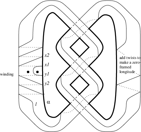
We may bring this Heegaard diagram into the form shown in Figure 8, where the surface is a connected sum of the torus and ; a surface of genus . We assume that and are the standard generators of the homology of , and that all other curves are on and are in the standard configuration such that by attaching a disk to these curves we get the handlebody formed by the inside of . The diagram gives a Heegaard diagram for the complement of the knot in and the neighborhood of may be identified with the interior of , since has zero linking number with the core of the torus .
If we embed the knot inside the torus and find a Heegaard diagram for its complement, this Heegaard diagram together with the Heegaard diagram for will give a diagram for the double of the knot in .
More precisely, consider the Heegaard diagram shown in Figure 8 (b) for the unknot sitting inside the solid torus. Here the thick curves denote the circles, while the thin ones are ’s. There is an extra curve shown in the picture, which we save for the later purposes. There is a special -curve denoted by in the figure, which represents the generator of the first homology group of the solid torus.
If we attach a disk to each curve, except for , in this Heegaard diagram and a disk to each of the circles other than the meridian , we will get the complement of the knot inside a solid torus .
Put this solid torus inside the torus . Attach the surface of the solid torus and by a one-handle connecting the intersection of and on to the intersection of and on the Heegaard diagram for .
The result of this operation may be regarded as a connected sum of the surfaces and . Here is the above Heegaard diagram for , and is the surface in the Heegaard diagram of used above.
Denote by the curves on and by the curves, as is shown in Figure 8 (b).
 .
.In order to find a Heegaard diagram for the complement of the Whitehead double in the sphere , we have to fill the space between the solid torus and the torus . Looking at , there are two disks which sit in the empty space between and the solid torus. Namely, if we cut the union by a horizontal plane, the intersection will look like the left hand side of Figure 9. There is a disk bounded by the connected sum . This disk is dashed in Figure 9.
We may also cut the torus with a vertical plane. If the cut is made in a way that it passes through and , and cuts the handle connecting the solid torus and the torus , then the cut will look like what is shown on the right hand side of Figure 9. Again, there is a disk which is dashed in the picture, with a boundary which is the connected sum .
The result of this operation is a Heegaard diagram for the Whitehead double of :
where and are two base points which are put on the two sides of the curve on . We will use this Heegaard diagram to relate the Ozsváth-Szabó Floer homology of the Whitehead double of to the longitude Floer homology discussed in the earlier sections.
6 Whitehead double; homology computation
In order to obtain the Ozsváth-Szabó Floer homology groups we should first form the chain complex by identifying the relevant generators of this Heegaard diagram.
There are two types of generators for this Heegaard diagram:
(1)\quaThe Kauffman states which are in correspondence with a pair of generators of the form , where is a generator of
and is a generator of . We call these generators meridian Kauffman states.
(2)\quaThe Kauffman states which are associated with a pair of generators of the form , where is a generator of
and is a generator of . We call these generators the longitude Kauffman states.
If and are two meridian Kauffman states, the domain between on will have coefficient on one side and on the other side of the meridian . We may complete this domain to the domain of an actual disk connecting and by adding the domain on with the multiplicities shown in Figure 10 .
Therefore, any two meridian Kauffman states and are in the same class.
A similar argument using the periodic domain of and the above periodic domain of in Figure 10, shows that any two longitude Kauffman states and are also in the same class.

To understand the grading between meridian and longitude Kauffman states, the next step is to consider the Kauffman states of the two Heegaard diagrams
We have named the intersection points of the diagram by letters of the alphabet in Figure 10.
The Kauffman states of will be the following list
It is easy to see that and are in the same class and there is a disk between them, which is disjoint from the shaded area, where the handle is attached to the surface . This disk supports a unique holomorphic representative. The numbers in parenthesis denote the nonzero coefficients of the disk between these two Kauffman states.
The Kauffman state is in a higher class. This means that .
The relative Maslov grading of any two Kauffman states (of the meridian or longitude type) and is the same as the relative Maslov index of the states and . So the contribution of all the Kauffman states of the form , for a fixed , is equal (up to a sign) to the Euler characteristic of or the Euler characteristic of , depending on whether ’s are meridian Kauffman states or longitude Kauffman states, respectively. This implies that the total contribution of longitude Kauffman states to the Euler characteristic in different structures is zero. For each of we will get a contribution equal to . The contribution from is cancelled against the contribution from , so the only structure for which the contribution is nonzero, is . The conclusion is that , since the Euler characteristic of gives the symmetrized Alexander polynomial of (which is trivial). Moreover, as a result of the previous discussion, we have:
Here the right hand side is a class associated with the Heegaard diagram . So , and there is no meridian Kauffman state in the class .
Now we turn to the Kauffman states of . We will show that some of them naturally cancel against each other. Then we will identify the remaining ones, and will compute the -grading of the corresponding longitude Kauffman states.
There is a small rectangle bounded by the intersection points on the lower face of the surface. For any pair of Kauffman states for the Whitehead double which are of the form and , the domain of the disk between these two states is this rectangle, which supports a unique holomorphic representative. There are six of these pairs. We may cancel them against each other, in the expense that having two Kauffman states with a disk of the following type connecting them, we will not be able to argue that there is no boundary map between the two Kauffman states. The disks considered above are the ones with negative coefficients in the rectangle. Since we will not face this situation in what follows, we simply choose to cancel them against each other. For a more careful explanation of this method we refer the reader to Rasmussen’s paper [9].
Here is a list of the remaining Kauffman states:
One may check by considering the domains that
| (8) |
In order to see what the absolute grading of these states is, move ( the unique curve that intersects ) by an isotopy to create a pair of intersection points with . One of them has the property that together with the intersection of and and the intersection of and , they form the vertices of a small triangle. Call this point and let be the intersection point of and . If is a Kauffman state for , then will be a Kauffman state for
There is a domain representing a disk with zero coefficients on and which connects the two Kauffman states and . So for any longitude Kauffman state of the form we may compute the grading via the formula:
| (9) |
So the only Kauffman states in the structure that remain, are those of the form , where is some Kauffman state on the Heegaard diagram (which is a potential Heegaard diagram for the longitude Floer homology).
Suppose that and are two Kauffman states in our Heegaard diagram. Since the states do not differ on , the only possibility for a domain between the two states is that the coefficients in all of the regions on are zero except for the regions where a coefficient equal to is assigned as in Figure 10. In any such domain, there are regions with both and as coefficients. Furthermore, these domains do not use the small rectangle considered before. So the only case where there is potentially a boundary map from to is when we have .
In this case the four regions around the connecting handle will get coefficients equal to zero. This means that the disk is completely supported on . Furthermore if we put two marked points and on the two sides of at the intersection of with , the above discussion shows that the domains of the disks between these points will have zero coefficients in the regions associated with and .
So, the disks that contribute to the boundary operator are in 1-1 correspondence with the disks between and in the hat theory assigned to the Heegaard diagram
The above discussion shows that the generators and all the boundary maps in the Ozsváth-Szabó Floer homology of in structure are exactly the same as those appearing in
The grading of , and that of the homology groups are forgotten when we compute the Ozsváth-Szabó Floer homology of the Whitehead double, and the isomorphism is an isomorphism of groups (relatively) graded by the Maslov index.
We have proved the following theorem:
Theorem 6.1.
Let denote the Whitehead double of a knot in . The Ozsváth-Szabó Floer homology groups are isomorphic to the group as (relatively) -graded abelian groups with the (relative) grading on both sides coming from the Maslov grading.
As a corollary of this theorem and the results of the previous section we have:
Corollary 6.2.
Let denote the torus knot and let be the Whitehead double of . Then the Ozsváth-Szabó Floer homology groups in different (relative) Maslov gradings are described as follows:
Remark 6.3.
The longitude Floer homology may be defined for a knot in a three-manifold , and as such, it enjoys very nice surgery formulas. We postpone a discussion of these subjects to a future paper.
References
- [1] G Burde, H Zieschang, Knots, de Gruyter Studies in Mathematics 5, Walter de Gruyter & Co. Berlin (2003) \MR1959408
- [2] P Ozsváth, Z Szabó, Holomorphic disks and knot invariants, to appear in Advances in Math, \arxivmath.GT/0209056
- [3] P Ozsváth, Z Szabó, Heegaard Floer homology and alternating knots, \gtref720036225254 \MR1988285
- [4] P Ozsváth, Z Szabó, Holomorphic disks and topological invariants for closed three-manifolds, to appear in Annals of Math. \arxivmath.SG/0101206
- [5] P Ozsváth, Z Szabó, Holomorphic disks and three-manifold invariants: properties and applications, to appear in Annals of Math. \arxivmath.SG/0105202
- [6] P Ozsváth, Z Szabó, Heegaard Floer homologies and contact structures, \arxivmath.SG/0210127
- [7] P Ozsváth, Z Szabó, Knot Floer homology and the four-ball genus, \gtref7200317615639 \MR2026543
- [8] P Ozsváth, Z Szabó, Holomorphic disks and genus bounds, \gtref820048311334 \MR2023281
- [9] J A Rasmussen, Floer homology of surgeries on two-bridge knots, \agtref2200232757789 \MR1928176
- [10] textbfJ A Rasmussen, Floer homology and knot complements, PhD thesis, Harvard Univ. \arxivmath.GT/0306378
- [11] L Rudolph, The slice genus and the Thurston-Bennequin invariant of a knot, Proc. Amer. Math. Soc. 125 (1997) 3049–3050 \MR1443854
Received:\qua15 July 2004