Legendrian Solid-Torus LinksThanks: Ng is supported by a Five-Year Fellowship from the American Institute of Mathematics. Traynor was supported in part by NSF grant DMS 9971374.

Lenhard Ng Address: Department of Mathematics, Stanford University, Stanford, CA 94305 and Lisa Traynor Address: Department of Mathematics, Bryn Mawr College, Bryn Mawr, PA 19010

Abstract.

Differential graded algebra invariants are constructed for Legendrian links in the $1$ -jet space of the circle. In parallel to the theory for $\mathbb{R}^{3}$ , Poincaré–Chekanov polynomials and characteristic algebras can be associated to such links. The theory is applied to distinguish various knots, as well as links that are closures of Legendrian versions of rational tangles. For a large number of two-component links, the Poincaré–Chekanov polynomials agree with the polynomials defined through the theory of generating functions. Examples are given of knots and links which differ by an even number of horizontal flypes that have the same polynomials but distinct characteristic algebras. Results obtainable from a Legendrian satellite construction are compared to results obtainable from the DGA and generating function techniques.

1. Introduction

In the late 1990’s, there were some breakthrough ideas for constructing new invariants of Legendrian links in $\mathbb{R}^{3}$ . These invariants came from adapting the techniques of pseudoholomorphic curves, a powerful tool in the study of symplectic manifolds, to the setting of contact manifolds, via contact homology [EGH]. Combinatorial ways of calculating these “holomorphic” invariants were developed from both the Lagrangian and the front projections of a Legendrian link [Ch, ENS, Ng1].

In this paper, the focus will be to study links in the 1-jet space of the circle, $\mathcal{J}^{1}(S^{1})$ , a manifold diffeomorphic to the solid torus $S^{1}\times\mathbb{R}^{2}$ :

\mathcal{J}^{1}(S^{1})=T^{*}(S^{1})\times\mathbb{R}=\{(x,y,z)\,:\,x\in S^{1},\ y,z\in\mathbb{R}\},

with contact structure given by $\xi=\ker(dz-y\,dx)$ . Viewing $S^{1}$ as a quotient of the unit interval, $S^{1}=[0,1]/(0\sim 1)$ , we can visualize knots in $\mathcal{J}^{1}(S^{1})$ as quotients of arcs in $I\times\mathbb{R}^{2}$ with appropriate boundary conditions.

Links in $\mathcal{J}^{1}(S^{1})$ were examined by one of the authors using the technique of generating functions, [Tr]. In this paper holomorphic techniques are developed to study these and other links. In Section 2, the theory underlying the holomorphic invariants is developed. Given the “Lagrangian” $xy$ -projection of a Legendrian link in $\mathcal{J}^{1}(S^{1})$ , it is possible to combinatorially define the Chekanov–Eliashberg differential graded algebra (DGA) over $\mathbb{Z}_{2}$ , in a manner exactly following the definition in $\mathbb{R}^{3}$ from [Ch]. However, as in $\mathbb{R}^{3}$ , it is often more convenient to work in the “front” $xz$ -projection rather than the Lagrangian $xy$ -projection. To do this, we introduce a suitable modification of the resolution technique for $\mathbb{R}^{3}$ from [Ng1], which produces a Lagrangian projection from a front projection. Using this resolution, and in parallel to the $\mathbb{R}^{3}$ theory, we can associate to Legendrian links in $\mathcal{J}^{1}(S^{1})$ invariants such as Poincaré–Chekanov polynomials, which measure the homology of a linearized version of the Chekanov–Eliashberg DGA, and characteristic algebras, which measure some nonlinear information from the DGA. We also make use of the additional structure on the DGA provided by Mishachev’s homotopy splitting, [Mi]. For multi-component links, this results in split Poincaré–Chekanov polynomials and split characteristic algebras.

Natural knot candidates for study with this technique are formed by identifying the ends of long Legendrian knots in $\mathbb{R}^{3}$ . Figure 1 shows two distinct Legendrian knots that are similar in spirit to Chekanov’s $5_{2}$ examples. These can be distinguished by the Poincaré–Chekanov polynomials. More examples of this sort are explored in Section 3.

Refer to caption — Figure 1. Closures of long knot versions of Chekanov’s $5_{2}$ knots. These can be distinguished by the Poincaré–Chekanov polynomials.

Some natural link candidates for study are the families of links studied in [Tr]. Such links can be specified by a vector of the form

	$\displaystyle(2h_{n},v_{n-1},2h_{n-1}^{p_{n-1}},\dots,2h_{2}^{p_{2}},v_{1},2h_{1}^{p_{1}}),\quad$	$\displaystyle h_{n},v_{n-1},\dots,h_{2},v_{1}\geq 1,\quad h_{1}\geq 0,$
	$\displaystyle\text{ and }p_{i}\in$	$\displaystyle\{0,\dots,2h_{i}\}\text{ for }i\in\{1,\dots,n-1\}.$

These links can be seen as quotients of Legendrian versions of even parity rational tangles defined by Conway in [Co]. The superscripts denote a link obtained by “horizontal flypes” of a standard configuration. In Section 4, the Poincaré–Chekanov polynomials of these links are calculated. There is a striking parallel between the split Poincaré–Chekanov polynomials defined via the holomorphic technique and the signed polynomials defined via the generating function technique: after a change of variables, the positive Poincaré–Chekanov polynomial agrees with the negative generating function polynomial, see Remark 4.3. This gives evidence for the following principle, which seems to hold for other contact manifolds as well:

The following two Legendrian-isotopy invariants contain the same information, when defined:

•

Morse-theoretic Poincaré polynomials obtained from generating functions;
•

first-order Poincaré–Chekanov polynomials obtained from holomorphic curves and contact homology.

This principle has been verified for all solid-torus links for which generating function polynomials have been defined. At present, this does not include all solid-torus links, and so there are instances in which the linearized DGA is applicable but generating functions are not. In addition, we will present an example of two links for which the generating function polynomials are defined and equal, but which can be distinguished by the full DGA via characteristic algebras.

We now look at some concrete examples of links which can be distinguished by one means or another. The first example in Figure 2 gives topologically equivalent links that do not have the same polynomials (generating function or Poincaré–Chekanov) and are hence not Legendrian isotopic. The second example gives knots of a similar flavor that can also be distinguished by their polynomials. This knot example solves Question 1.34 posed in [Tr].

Theorems 4.2 and 4.5 show that the polynomials may detect the parity of the numbers of horizontal flypes. This raises interesting questions about links that differ by an even number of flypes. For example, Question 1.31 in [Tr] asks whether the Legendrian links denoted by $(2,1,2)\#(2,1,2)$ and $(2,1,2^{2})\#(2,1,2)$ shown in Figure 3 are isotopic.

In parallel to the generating function theory, the holomorphic polynomials of these (nonrational) connect sums of the form $L_{1}\#L_{2}$ can be easily calculated from the polynomials of $L_{1}$ and $L_{2}$ , see Theorem 5.1 and Remark 5.2. Thus the polynomials of $(2,1,2)\#(2,1,2)$ and $(2,1,2^{2})\#(2,1,2)$ agree. However, a calculation of their characteristic algebras shows that these are in fact distinct; see Proposition 5.6. A solution to this problem raises some new interesting questions. For example, a slight modification of the constructions in Figure 3 produces the knots in Figure 4 that have tamely isomorphic DGAs. Are these knots isotopic? This and some related questions are posed in Section 5.

We include a short appendix which describes a technique, different from the DGA or generating functions, which can also distinguish Legendrian solid-torus links. The relevant construction, which we call a Legendrian satellite, constructs a link in standard contact $\mathbb{R}^{3}$ from a link in the solid torus. We show that Legendrian satellites can be used to recover some of the results derived in this paper using the DGA or in [Tr] using generating functions, and can even be applied in cases where neither of the other techniques works.

Acknowledgments

We thank the American Institute of Mathematics for sponsoring the contact geometry program during Fall 2000, where the ideas for this paper originated. We also thank the hospitality of the Institute for Advanced Study in 2001–2002 when further ideas were developed.

2. Holomorphic Invariants

2.1. The DGA invariant

As in standard contact $\mathbb{R}^{3}$ , apart from topological type, oriented Legendrian links in $\mathcal{J}^{1}(S^{1})$ have two classical contact invariants, rotation number $r$ and Thurston–Bennequin number $tb$ . These are defined in precisely the same way as in $\mathbb{R}^{3}$ ; for instance, in the “front” $xz$ -projection, $2r$ is the number of cusps oriented downwards minus the number oriented upwards, and $tb$ is the number of crossings, counted with the usual signs, minus the number of right cusps. In [Ch], inspired by work of Eliashberg and Hofer, Chekanov introduced a nonclassical invariant of Legendrian knots in $\mathbb{R}^{3}$ , and we will be interested in its analogue in $\mathcal{J}^{1}(S^{1})$ .

Given the “Lagrangian” $xy$ -projection of a Legendrian link in $\mathcal{J}^{1}(S^{1})$ , we may combinatorially define the Chekanov–Eliashberg differential graded algebra $(\mathbb{A},\partial)$ in a manner exactly following the definition in $\mathbb{R}^{3}$ from [Ch, ENS]. All proofs translate, without changes, to solid-torus links. We summarize here the main results about the DGA; please refer to one of [Ch, ENS, Ng1] for definitions of terms.

Theorem 2.1.

$\partial^{2}=0$ , and $\partial$ lowers degree by $1$ .

Theorem 2.2.

Two Legendrian-isotopic links in $\mathcal{J}^{1}(S^{1})$ have equivalent DGAs.

As will be explained in more detail below, all of the algebraic machinery built around DGAs, including Poincaré polynomials [Ch] and characteristic algebras [Ng1], can be applied to our setup. However, as in standard contact $\mathbb{R}^{3}$ , it is often more convenient to work in the front projection rather than the Lagrangian projection. The following resolution technique, a slight modification of that used in $\mathbb{R}^{3}$ in [Ng1], tells us how to do the “bookkeeping” when working in the front projection. Using resolution, we will then define the Chekanov–Eliashberg DGA for fronts of Legendrian links in $\mathcal{J}^{1}(S^{1})$ .

2.2. Resolution

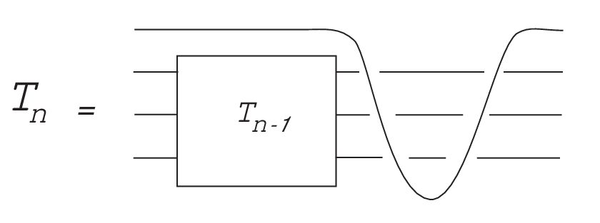
To convert an $xz$ -projected Legendrian link to an $xy$ -projected link, we use resolution, as in [Ng1]. Figure 5 illustrates for the link with an $xz$ -projection consisting of two line segments of slope zero how in the resolution procedure the front diagram is modified so that initially the upper strand has slope $1$ . As seen in this case, a complication not present in the $\mathbb{R}^{3}$ case is that after the normal resolution procedure, in order for the strands to close up smoothly under the identification, a “transition” tangle (with no crossings) needs to be adjoined to the $xz$ -projection. In the $xy$ -projection, this translates into adjoining a topologically trivial tangle $T_{n}$ , with $n$ strands, defined inductively as follows: $T_{1}$ is the trivial tangle with $1$ strand, and $T_{n}$ is obtained from $T_{n-1}$ through the construction shown in Figure 6.

Definition 2.3.

Let $Z$ be the front projection of a Legendrian link in $S^{1}\times\mathbb{R}^{2}$ . The resolution of $Z$ is the Lagrangian projection of a Legendrian link obtained by resolving each singularity as in Figure 7, and appending a tangle $T_{n}$ at the very right of the projection, as given in Figure 6, for appropriate $n$ . See Figure 8 for an example.

Proposition 2.4.

Let $Z$ be the front projection of a Legendrian link $L$ and let $Y$ be its resolution. Then $Y$ is the Lagrangian projection of a Legendrian link $L^{\prime}$ that is Legendrian isotopic to $L$ .

Proof.

The corresponding proof in $\mathbb{R}^{3}$ from [Ng1] distorts the front, starting at the left and moving right, so that the Lagrangian projection of the associated Legendrian link is the resolution of the front. This proof works here until we reach the right end of the front. In order to connect smoothly with the left end of the front, we need to move the right end so that it will close up with the left end under the identification. If we label the strands on the right end of the front by $1,\ldots,n$ in order of increasing $z$ coordinate, then we interpolate a segment of nonpositive slope into strand $1$ so that it will close up under the identification; next we interpolate a segment of more negative slope into strand $2$ so that it will also close up; and so on. See Figure 9. The resulting Lagrangian projection contains the tangle $T_{n}$ on its right, and is precisely the resolution of the original front. ∎

To calculate the DGA of a Legendrian link $L$ in $\mathcal{J}^{1}(S^{1})$ , it will be convenient to use a diagram that is a combination of the front and Lagrangian projections. First we set some notation. Consider the projection obtained from the front projection $Z$ of $L$ by formally appending on the right the tangle $T_{n}$ for appropriate $n$ . We will call this the resolved front projection and will often denote it by $Z^{\prime}$ . See Figure 10. Define the vertices of $Z^{\prime}$ to be its crossings (including the crossings in $T_{n}$ ) and right cusps, and label the vertices by $a_{1},\ldots,a_{k}$ . The term normal crossing will be used for vertices in the front projection and for crossings in $T_{n}$ that appear with the overstrand having lesser slope. A special crossing will denote a crossing in $T_{n}$ where the overstrand has greater slope. In the resolved front projection, all special crossings will be drawn with a broken segment to denote the understrand, to emphasize the fact that these are the only crossings which are not resolved by having the strand with lesser slope be the overstrand.

The DGA for $L$ is $(\mathbb{A},\partial)$ , where $\mathbb{A}$ is the free, noncommutative, unital algebra generated by $a_{1},\ldots,a_{k}$ , with grading to be described in Section 2.3, and $\partial$ is defined over $\mathbb{Z}/2$ by the following procedure. As in [Ch] and [Ng1], we define $\partial(a_{i})$ for a generator $a_{i}$ by considering a certain class of immersed disks in the resolved front projection $Z^{\prime}$ .

Definition 2.5.

An admissible map in $Z^{\prime}$ is an immersion from the $2$ -disk $D^{2}$ to $\mathbb{R}^{2}$ which maps the boundary of $D^{2}$ into $Z^{\prime}$ , and which satisfies the following properties: the image of the map near any singularity looks locally like one of the diagrams in Figure 11, and, in the notation of Figure 11, there is precisely one initial vertex.

Note that Figure 11 is quite similar to Figure 5 in [Ng1] except that due to the special vertices in the tangle $T_{n}$ , there are additional possibilities for initial vertices and corner vertices. Note that the “forbidden singularity” was also forbidden in [Ng1]. Here it is forbidden since if some disk involves this singularity, then it has a rightmost negative corner (at one of the special crossings), but one can check that any disk with a rightmost negative corner at a special crossing has to remain within the tangle $T_{n}$ and thus cannot “escape” the tangle on the left to reach the cusp singularity.

For each admissible map with initial vertex at $a_{i}$ , we can read off the singularities of the boundary of the disk counterclockwise, beginning just after $a_{i}$ and ending just before reaching $a_{i}$ again. Count each of the singularities $0$ , $1$ , or $2$ times, depending on which singularity it depicts in Figure 11. Concatenating the labels for the singularities, with multiplicity, yields a word in $\mathbb{A}$ , which we associate to the disk. We then define $\partial a_{i}$ to be the sum of these words over all admissible maps with initial vertex at $a_{i}$ , or $1$ plus this sum if $a_{i}$ is a right cusp.

As is usual, we can extend $\partial$ to all of $\mathbb{A}$ via the Leibniz rule. It is straightforward to check that the usual definition of the DGA for Lagrangian projections translates to our definition for fronts. Theorems 2.1 and 2.2 then imply that $\partial^{2}=0$ and that the DGA $(\mathbb{A},\partial)$ is, up to equivalence, a Legendrian-isotopy invariant of $L$ .

For example, for the resolved front in Figure 10, we have

$\displaystyle\partial a_{1}$	$\displaystyle=1+a_{9}a_{2}+a_{8}a_{3}$	$\displaystyle\quad\quad\partial a_{4}$	$\displaystyle=a_{3}+a_{5}$	$\displaystyle\quad\quad\partial a_{7}$	$\displaystyle=a_{6}a_{5}+a_{2}+a_{5}a_{4}+a_{8}$
$\displaystyle\partial a_{2}$	$\displaystyle=a_{5}a_{3}$	$\displaystyle\partial a_{5}$	$\displaystyle=0$	$\displaystyle\partial a_{8}$	$\displaystyle=a_{9}a_{5}$
$\displaystyle\partial a_{3}$	$\displaystyle=0$	$\displaystyle\partial a_{6}$	$\displaystyle=a_{5}+a_{9}$	$\displaystyle\partial a_{9}$	$\displaystyle=0.$

Remark 2.6.

As in [ENS, Ng1], we may also lift the DGA to an algebra over a ring of the form $\mathbb{Z}[t_{1},t_{1}^{-1},\ldots,t_{m},t_{m}^{-1}]$ , graded over $\mathbb{Z}$ . Since we currently have no applications of this lifted DGA, we will omit its definition here.

At times, it will be convenient to restrict our attention to a special class of fronts; as in [Ng1], it is easy to Legendrian-isotop any front into the form described below.

Definition 2.7.

Any front in $\mathcal{J}^{1}(S^{1})$ that represents a nontrivial element of $\pi_{1}(\mathcal{J}^{1}(S^{1}))$ divides the cylinder $S^{1}\times\mathbb{R}$ into several regions, including two unbounded ones, one above, one below the front. We call a front simple if each of its right cusps lies on the boundary of one of these unbounded regions.

The front in Figure 8 is simple, while the front in Figure 15 below is not. For simple fronts, the vertices labeled with III in Figure 11 do not occur and thus it follows that the boundary map for the generators $a_{i}$ can be calculated in terms of embedded (rather than immersed) disks in the resolved front diagram.

2.3. Gradings

In the previous section, we defined the Chekanov–Eliashberg DGA associated to a Legendrian front in $\mathcal{J}^{1}(S^{1})$ , except for the grading on the algebra; we now address the issue of gradings. In [Ch], Chekanov defined a grading for generators of the DGA of a link in $\mathbb{R}^{3}$ . Following [Ng1], we will describe how to define the degrees of vertices in a resolved front projection in $\mathcal{J}^{1}(S^{1})$ .

For knots, the grading is well-defined, but for links, it depends on the choice of some auxiliary points on each component of the link; changing one of the points shifts some of the indices by some integer. The cases of interest to us will be knots and particular links for which there is a canonical way to choose auxiliary points. We address these cases in turn; the definition of gradings for a general link, which we omit here, can be inferred from the corresponding definition for links in $\mathbb{R}^{3}$ in [Ng1].

For the front of a Legendrian knot in $\mathcal{J}^{1}(S^{1})$ , we can define the grading on the DGA as follows. The degree of each right cusp is $1$ . For a crossing $a$ in the resolved front projection, traverse the knot beginning at the greater-slope strand at the crossing, and ending when the crossing is reached again, and let $c(a)$ be the number of cusps traversed upwards minus the number traversed downwards. If $a$ is a normal crossing, then $\deg a=c(a)$ ; if $a$ is a special crossing, then $\deg a=-c(a)-1$ . By extending degree multiplicatively (i.e., $\deg(ab)=\deg a+\deg b$ ), this determines a $\mathbb{Z}/(2r)$ grading on the DGA, where $r$ is the rotation number of the knot.

Now suppose instead that we are given a Legendrian link $L=(\Lambda_{1},\dots,\Lambda_{n})$ in $\mathcal{J}^{1}(S^{1})$ , such that each component $\Lambda_{i}$ is Legendrian isotopic to the $1$ -jet (in the front projection, the graph) of a function. We will see that there is a canonical way to choose an auxiliary point on each component, and hence the DGA for $L$ can be given a natural grading which is unique.

Definition 2.8.

Given a Legendrian knot $\Lambda\subset\mathcal{J}^{1}(S^{1})$ , the branches of $\Lambda$ are the connected components of $\Lambda\backslash C$ , where $C$ denotes the set of points that front-project to cusps. Suppose further that $\Lambda\subset\mathcal{J}^{1}(S^{1})$ is Legendrian isotopic to the $1$ -jet of the $0$ -function, $j^{1}(0)$ . A branch $\mathcal{I}$ is called initial if there exists $v\in\mathcal{I}$ and a contact isotopy $\kappa_{t}$ of $\mathcal{J}^{1}(S^{1})$ , $t\in[0,1]$ , so that $\kappa_{0}=\textrm{id}$ , $\kappa_{1}(\Lambda)=j^{1}(0)$ , and $\kappa_{t}(v)$ never front-projects to a cusp (including the singular point of a “Reidemeister type I” move in the isotopy which creates or destroys two cusps and a crossing).

For each crossing $a_{i}$ , let $N^{o}(a_{i})$ and $N^{u}(a_{i})$ denote neighborhoods of $a_{i}$ on the two strands intersecting at $a_{i}$ with $N^{o}(a_{i})$ being a portion of the overstrand. Note that for a normal crossing, $N^{o}(a_{i})$ will be in the strand of lesser slope. For each $j=1,\dots,k$ , fix a base point $p_{j}$ on an initial branch of $\Lambda_{j}$ , and let $P=\{p_{1},\dots,p_{k}\}$ denote this set of base points.

To each crossing, we associate two “capping paths” $\gamma_{i}^{o},\gamma_{i}^{u}$ : $\gamma_{i}^{o}$ is a path from $a_{i}$ through $N^{o}(a_{i})$ to a point in $P$ while $\gamma_{i}^{u}$ is a path from $a_{i}$ through $N^{u}(a_{i})$ to a point in $P$ . For each such path $\gamma$ , let $c(\gamma)$ denote the number of up cusps minus the number of down cusps along the path.

Definition 2.9.

Suppose $L=(\Lambda_{1},\dots,\Lambda_{n})$ where $\Lambda_{i}$ is Legendrian isotopic to the $1$ -jet of a function. Then

\deg(a_{i})=\begin{cases}1,&a_{i}\text{ a right cusp}\\ c(\gamma_{i}^{u})-c(\gamma_{i}^{o}),&a_{i}\text{ a normal crossing}\\ c(\gamma_{i}^{u})-c(\gamma_{i}^{o})-1,&a_{i}\text{ a special crossing.}\end{cases}

As usual, degree extends to the entire algebra by multiplicativity.

Lemma 2.10.

The degree function does not depend on the choice of paths $\gamma_{i}^{o}$ , $\gamma_{i}^{u}$ , nor on the choice of marked points on initial branches.

Proof.

Since each component $\Lambda_{i}$ of the link is Legendrian isotopic to $j^{1}(0)$ , each component must contain equal numbers of up and down cusps. It is then easy to check that $\deg(a_{i})$ does not depend on the choice of paths $\gamma_{i}^{o}$ , $\gamma_{i}^{u}$ . In addition, Proposition 5.3 in [Tr] shows that a path between any two points in initial branches contains an equal number of up and down cusps. Thus the degree function does not depend on the choice of points in initial branches. ∎

Notice that for any Legendrian isotopy of a link $L=(\Lambda_{1},\dots,\Lambda_{k})$ , a choice of base points on initial branches for the original link yields a choice of base points on initial branches throughout the isotopy. It follows that the degree given above makes the DGA of the link a Legendrian-isotopy invariant.

For both knots and the links we have considered in this section, we have the following result, whose proof can (essentially) be found in [Ch].

Proposition 2.11.

$\partial$ lowers degree by $1$ .

2.4. Link DGAs

In addition to the grading of the differential algebra, there is a structure on the DGA for a link $L$ given by Mishachev’s relative homotopy splitting [Mi]; see [Ng1] for the formulation we present here. For a link $L=(\Lambda_{1},\dots,\Lambda_{k})$ , we can split something which is essentially a submodule of the DGA into $k^{2}$ pieces which are invariant under Legendrian isotopy. This additional structure will be useful in applying the DGA to distinguish between links.

Recall that for a crossing $a$ , $N^{o}(a)$ and $N^{u}(a)$ denote neighborhoods of $a$ in the overstrand and understrand.

Definition 2.12.

For $L=(\Lambda_{1},\dots,\Lambda_{k})$ , let $j_{1},j_{2}\in\{1,\dots,k\}$ . If $j_{1}\neq j_{2}$ , define $\mathbb{A}^{j_{1}j_{2}}$ to be the module over $\mathbb{Z}/2$ generated by words of the form $a_{i_{1}}\cdots a_{i_{m}}$ where $N^{o}(a_{i_{1}})\subset\Lambda_{j_{1}}$ , $N^{u}(a_{i_{m}})\subset\Lambda_{j_{2}}$ , and for $1\leq p<m$ , $N^{u}(a_{i_{p}})$ and $N^{o}(a_{i_{p+1}})$ belong to the same component of $L$ . For $j_{1}=j_{2}=j$ , let $\mathbb{A}^{j_{1}j_{2}}$ be the module generated by such words, together with an indeterminate $e_{j}$ . Then let $\mathbb{A}^{**}=\oplus\mathbb{A}^{j_{1}j_{2}}$ .

Each $1$ term in the definition of $\partial$ will be replaced by an $e_{j}$ term; see below. Note that a generator $a$ is in $\mathbb{A}^{jk}$ if and only if $N^{o}(a)\subset\Lambda_{j}$ and $N^{u}(a)\subset\Lambda_{k}$ .

There is an algebra structure on $\mathbb{A}^{**}$ , where multiplication is defined by the following map $\mathbb{A}^{j_{1}j_{2}}\times\mathbb{A}^{j_{3}j_{4}}\rightarrow\mathbb{A}^{j_{1}j_{4}}$ : the map is $0$ unless $j_{2}=j_{3}$ , in which case it is given on generators by concatenation, with the $e_{j}$ terms acting as the identity. There exists a differential on $\mathbb{A}^{**}$ which is a slight variation of $\partial$ . Define $\partial^{\prime}a_{i}$ on the generators $a_{i}$ of $\mathbb{A}^{**}$ as follows: if $N^{o}(a_{i})$ and $N^{u}(a_{i})$ are contained in distinct components of $L$ , then $\partial^{\prime}a_{i}=\partial a_{i}$ ; if $N^{o}(a_{i})$ and $N^{u}(a_{i})$ are contained in the same component $\Lambda_{j}$ of $L$ , replace any $1$ term by $e_{j}$ . It is easy to see (cf. [Ng1]) that $\partial^{\prime}$ preserves $\mathbb{A}^{j_{1}j_{2}}$ for any $j_{1},j_{2}$ .

Definition 2.13.

The link DGA of $L=(\Lambda_{1},\dots,\Lambda_{k})$ is $(\mathbb{A}^{**},\partial^{\prime})$ , where $\partial^{\prime}a_{i}$ is defined above, and we extend $\partial^{\prime}$ to $\mathbb{A}^{**}$ by applying the Leibniz rule and setting $\partial^{\prime}e_{j}=0$ for all $j$ . $\mathbb{A}^{**}$ inherits a grading from the DGA of $L$ with $\deg e_{j}=0$ for all $j$ .

We may define grading-preserving elementary and tame automorphisms for link DGAs as for DGAs, with the additional stipulation that all maps must preserve the link structure by preserving $\mathbb{A}^{j_{1}j_{2}}$ for all $j_{1},j_{2}$ . Similarly, we may define an algebraic stabilization of a link DGA, with the additional stipulation that the two added generators both belong to the same $\mathbb{A}^{j_{1}j_{2}}$ . As usual, we then define two link DGAs to be equivalent if they are tamely isomorphic after some number of algebraic stabilizations.

Proposition 2.14.

If $L$ and $L^{\prime}$ are Legendrian isotopic oriented links, then the link DGAs for $L$ and $L^{\prime}$ are equivalent.

As in [Ng1], one can define a link characteristic algebra from a link DGA, which is also a Legendrian-isotopy invariant up to equivalence. This is defined to be the quotient of $\mathbb{A}^{**}$ by the subalgebra generated by the image of $\partial^{\prime}$ .

2.5. Split Poincaré–Chekanov polynomials

As in [Mi, Ng1], we can derive a set of first-order Poincaré–Chekanov polynomials from the link DGA. To do this, we will first need the notion of an augmentation for a link. Recall that an augmentation for a knot consists of an algebra map $\varepsilon:\mathbb{A}\to\mathbb{Z}/2$ where $\mathbb{A}$ is the DGA over $\mathbb{Z}/2$ for the knot, $\varepsilon\circ\partial=0$ , $\varepsilon(1)=1$ , and $\varepsilon$ vanishes for any element of nonzero degree.

Definition 2.15.

Suppose that each component $\Lambda_{i}$ of $L=(\Lambda_{1},\dots,\Lambda_{k})$ when considered as a knot has an augmentation $\varepsilon_{i}$ . Extend these augmentations to all vertices $a_{i}$ of $L$ by setting

\varepsilon(a_{i})=\begin{cases}\varepsilon_{j}(a_{i}),&\text{ if }a_{i}\in\mathbb{A}^{jj}\text{ for some }j,\\ 0,&\text{ otherwise.}\end{cases}

An augmentation of $L$ is any function $\varepsilon$ obtained in this way.

An augmentation $\varepsilon$ , as usual, gives rise to a first-order Poincaré–Chekanov polynomial $\chi_{\varepsilon}(\lambda)$ ; this polynomial splits into $k^{2}$ polynomials $\chi_{\varepsilon}^{j_{1}j_{2}}(\lambda)$ corresponding to the pieces in $\mathbb{A}^{j_{1}j_{2}}$ . More precisely, in the expression for $\partial a_{i}$ , replace each $a_{j}$ by $a_{j}+\varepsilon(a_{j})$ ; the result has no zero-order term in the $a_{j}$ , and we denote the first-order term by $\partial^{1}_{\varepsilon}(a_{j})$ . Then $\partial^{1}$ is a differential on the graded vector space $V_{*}$ over $\mathbb{Z}/2$ generated by the $a_{i}$ , and it preserves the subspaces $V_{*}^{j_{1}j_{2}}$ generated by the $a_{i}\in\mathbb{A}^{j_{1}j_{2}}$ .

Definition 2.16.

For each augmentation $\varepsilon$ , let

\beta_{k}^{j_{1}j_{2}}(\varepsilon)=\dim\frac{\ker\partial_{\varepsilon}^{1}:V_{k}^{j_{1}j_{2}}\to V_{k-1}^{j_{1}j_{2}}}{\operatorname{im}\partial_{\varepsilon}^{1}:V_{k+1}^{j_{1}j_{2}}\to V_{k}^{j_{1}j_{2}}}.

We define the split Poincaré–Chekanov polynomials of the link $L$ with respect to $\varepsilon$ to be

\chi_{\varepsilon}^{j_{1}j_{2}}(\lambda)[L]=\sum_{k}\beta_{k}^{j_{1}j_{2}}(\varepsilon)\lambda^{k}.

In the case when $L$ is a knot, there is just one polynomial per augmentation, which we call the Poincaré–Chekanov polynomial and denote $\chi_{\varepsilon}(\lambda)[L]$ .

Of course, the split polynomials depend on a choice of grading of the link, which is ambiguous in general but is well-defined for the cases which are of interest to us. The importance of the split Poincaré–Chekanov polynomials derives from the following result.

Proposition 2.17.

If $L$ is a knot, then the set of Poincaré–Chekanov polynomials for all possible augmentations of $L$ is invariant under Legendrian isotopy. If $L$ is a link whose components are all Legendrian isotopic to $j^{1}(0)$ , then for any $j_{1},j_{2}$ , the set of split Poincaré–Chekanov polynomials $\chi_{\varepsilon}^{j_{1}j_{2}}(\lambda)[L]$ for all possible augmentations $\varepsilon$ of a link $L$ is invariant under Legendrian isotopy.

Proof.

See [Ch, Ng1]; note that a similar result holds for arbitrary Legendrian links in $\mathcal{J}^{1}(S^{1})$ . ∎

If a knot or link has only one Poincaré–Chekanov polynomial, then we will sometimes suppress the subscript $\varepsilon$ and write $\chi(\lambda)[L]$ or $\chi^{j_{1}j_{2}}(\lambda)[L]$ .

We finish this section by noting one obvious property of split Poincaré–Chekanov polynomials, also mentioned in [Ng1], which we will use later.

Proposition 2.18.

For $L=(\Lambda_{1},\Lambda_{2},\dots,\Lambda_{k})$ , let $\sigma$ be a permutation of $\{1,\dots,k\}$ and consider $L_{\sigma}=(\Lambda_{\sigma(1)},\dots,\Lambda_{\sigma(k)})$ . Then if $L$ has a unique Poincaré–Chekanov polynomial,

\chi^{\sigma(j_{1})\sigma(j_{2})}(\lambda)[L_{\sigma}]=\chi^{j_{1}j_{2}}(\lambda)[L].

3. Legendrian Knots in the Solid Torus

In this section, we give several examples of Legendrian knots in the solid torus that can be distinguished using the DGA invariant. Note that the generating-function results from [Tr], which apply only to two-component links, cannot be used here.

A large class of Legendrian knots in $\mathcal{J}^{1}(S^{1})$ can be obtained by identifying the ends of long Legendrian knots in $\mathbb{R}^{3}$ (for a treatment of long Legendrian knots, see [Ch]). More precisely, given the front of a long Legendrian knot in standard contact $\mathbb{R}^{3}$ , say with ends asymptotic to the $x$ -axis, we can identify the two ends to produce the front of a Legendrian knot in $\mathcal{J}^{1}(S^{1})$ ; see, for example, the top pair of diagrams in Figure 12, which are derived from long-knot versions of the Chekanov $5_{2}$ knots. It is clear from the resolution construction of Section 2.2 that the DGA for the solid-torus knot is identical to the DGA of the long knot. One can then use Poincaré–Chekanov polynomials or other techniques to distinguish these solid-torus knots.

As an example, consider the top pair of knots in Figure 12. One can compute, either directly or using [Ch, Thm. 12.4] and the standard calculation of the polynomials for the Legendrian $5_{2}$ knots, that the knots, and their long-knot equivalents, have Poincaré–Chekanov polynomial $\chi(\lambda)=2$ (left knot) and $\chi(\lambda)=\lambda^{2}+\lambda^{-2}$ (right knot); hence they are not Legendrian isotopic.

Another pair of solid-torus knots related to the $5_{2}$ knots, but not derived from long knots, is the middle pair of knots in Figure 12, which we will call $K_{1}$ and $K_{2}$ . Both $K_{1}$ and $K_{2}$ have $r=0$ and $tb=1$ . With crossings as marked in Figure 13, the DGAs of $K_{1}$ and $K_{2}$ are defined by:

K_{1}:~~~\begin{aligned} \partial(a_{1})&=1+(1+a_{5}a_{4})a_{2}\\ \partial(a_{3})&=1+(1+a_{4}a_{5})a_{7}\\ \partial(a_{6})&=a_{2}+a_{7}\\ \partial(a_{i})&=0,~~~i\neq 1,3,6\end{aligned}\hskip 36.135ptK_{2}:~~~\begin{aligned} \partial(a_{1})&=1+(1+a_{4}a_{5})a_{2}\\ \partial(a_{3})&=1+a_{7}(1+a_{5}a_{4})\\ \partial(a_{6})&=a_{2}+a_{7}\\ \partial(a_{i})&=0,~~~i\neq 1,3,6.\end{aligned}

The key difference between the DGAs for $K_{1}$ and $K_{2}$ is that for $K_{1}$ , $\deg(a_{4})=\deg(a_{5})=0$ , while for $K_{2}$ , $\deg(a_{4})=2$ and $\deg(a_{5})=-2$ . We can then calculate the Poincaré–Chekanov polynomials to be $\chi(\lambda)[K_{1}]=\lambda+2$ and $\chi(\lambda)[K_{2}]=\lambda^{2}+\lambda+\lambda^{-2}$ . It follows that $K_{1}$ and $K_{2}$ are not Legendrian isotopic.

Using variants of the construction which gives $K_{1}$ and $K_{2}$ , one can produce many other examples of pairs of nonisotopic Legendrian knots. For instance, the bottom pair of knots in Figure 12 is a slightly more complicated example but can also be distinguished using the Poincaré–Chekanov polynomial.

We note that there are other ways to distinguish all of the example pairs in this section. One way is the method of Legendrian satellites (see the Appendix). A second way to distinguish these pairs is to adapt the generating function techniques developed for links in [Tr] to the knot setting; such calculations are done in [Jo].

The pair in the second example in Figure 12 can be viewed as quotients of Legendrian versions of infinite parity rational tangles. Quotients of Legendrian versions of even and odd parity rational tangles are studied in the next section.

4. Rational Links and Knots

In this section, we will calculate the split Poincaré–Chekanov polynomials of the two-component links studied in [Tr] and compare these polynomials to the polynomials defined via the theory of generating functions. These links can be seen as quotients of Legendrian versions of the even parity rational tangles defined by Conway in [Co]. Some (knot) quotients of Legendrian versions of odd parity rational tangle will also be examined, thus leading to solutions of some problems posed in [Tr].

The standard rational Legendrian link $(2h_{n},v_{n-1},\dots,2h_{2},v_{1},2h_{1})$ is a two-component link that can be constructed recursively: for $n=1$ , the links $(2h)$ have a front consisting of the graphs of two functions $f,g:S^{1}\to\mathbb{R}$ that intersect transversally at $2h$ points; for $n\geq 2$ , the $(2n-1)$ -length link $(2h_{n},v_{n-1},\dots,2h_{2},v_{1},2h_{1})$ is formed from “vertical and horizontal additions” to the $(2n-3)$ -length link $(2h_{n},\dots,v_{2},2h_{2})$ , as shown in Figure 14. For these two-component links $(\Lambda_{1},\Lambda_{2})$ , the top/darker strand depicted in Figure 14 will denote the second component. For all these links, it will be shown that the split Poincaré–Chekanov polynomials are unique and thus the set notation will be dropped.

The polynomials $\chi^{11}(\lambda)[L]$ and $\chi^{22}(\lambda)[L]$ are the usual Poincaré–Chekanov polynomials for each individual link component. Since, by construction, each component is isotopic to the $1$ -jet of a function, $\chi^{11}(\lambda)[L]=\chi^{22}(\lambda)[L]=0$ . However, the polynomials $\chi^{21}(\lambda)[L]$ and $\chi^{12}(\lambda)[L]$ will carry useful information.

Definition 4.1.

For a Legendrian link $L=(\Lambda_{1},\Lambda_{2})$ , define

\chi^{-}(\lambda)[L]=\chi^{21}(\lambda)[L],\qquad\chi^{+}(\lambda)[L]=\chi^{12}(\lambda)[L].

Throughout this section, as in [Tr], $\overline{p(\lambda)}$ denotes $p(\lambda^{-1})$ for any polynomial $p$ .

Theorem 4.2.

Consider the Legendrian link $L=(2h_{n},v_{n-1},\dots,v_{1},2h_{1})$ . Then

	$\displaystyle\chi^{+}(\lambda)[L]$	$\displaystyle=h_{1}+h_{2}\lambda^{v_{1}}+h_{3}\lambda^{v_{1}+v_{2}}+\dots+h_{n}\lambda^{v_{1}+\dots+v_{n-1}},$
	$\displaystyle\chi^{-}(\lambda)[L]$	$\displaystyle=\begin{cases}\overline{\chi^{+}(\lambda)[L]},&h_{1}\geq 1\\ \lambda^{-1}+1+\overline{\chi^{+}(\lambda)[L]},&h_{1}=0.\end{cases}$

Proof.

First consider the case of $h_{1}>0$ . Draw the link in standard (nonsimple) position as illustrated in Figure 15. This resolved front projection gives rise to a link DGA with

•

$2h_{1}+\dots+2h_{n}$ generators arising from the horizontal crossings; these will be denoted by

	$\displaystyle h_{j_{i}}^{\pm},\quad$	$\displaystyle j\in\{1,\dots,n\},\ i\in\{1,\dots,h_{j}\},$
	with	$\displaystyle\deg(h_{1_{i}}^{\pm})=0,\ \deg(h_{j_{i}}^{\pm})=\pm\sum_{k=1}^{j-1}v_{k},\quad h_{j_{i}}^{+}\in\mathbb{A}^{12},h_{j_{i}}^{-}\in\mathbb{A}^{21};$

•

$v_{1}+\dots+v_{n-1}$ generators arising from the vertical crossings; these will be denoted by

	$\displaystyle v_{j_{i}},\quad$	$\displaystyle j\in\{1,\dots,n-1\},\ i\in\{1,\dots,v_{j}\},$
		$\displaystyle\text{\ with\ }\deg(v_{j_{i}})=0,\quad v_{j_{i}}\in\mathbb{A}^{11};$

•

$(v_{1}-1)+\dots+(v_{n-1}-1)$ generators arising from the cusps that occur when $v_{i}>1$ ; these will be denoted by

	$\displaystyle m_{j_{i}},\quad$	$\displaystyle j\in\{1,\dots,n-1\},\ i\in\{1,\dots,v_{j}-1\},$
		$\displaystyle\text{\ with\ }\deg(m_{j_{i}})=1,\quad m_{j_{i}}\in\mathbb{A}^{11};$

•

$n-1$ generators arising from the cusps that occur when connecting the string of $v_{i}$ crossings with the string of $h_{i+1}$ crossings; these will be denoted by

$\displaystyle c_{j},\quad j\in\{1,\dots,n-1\},\quad\text{\ with\ }\deg(c_{j})=1,\quad c_{j}\in\mathbb{A}^{11};$
•

$2$ generators arising from the crossings that occur in the tangle $T_{2}$ ; these will be denoted by

$\displaystyle t_{0}^{-},t_{-1}^{-},\text{\ with\ }\deg(t_{k}^{-})=k,\quad t_{k}^{-}\in\mathbb{A}^{21}.$

Note that to calculate the degrees above, we can set base points on the two components of $L$ to be the “leftmost” points on the fronts, which certainly lie on initial branches.

There is a unique augmentation for the link given by $\varepsilon(v_{j_{i}})=1$ for all $j_{i}$ and $\varepsilon(a)=0$ for all other vertices. The augmented vertices (with $\varepsilon=1$ ) are denoted with double circles in Figure 15. To calculate $\chi^{\pm}(\lambda)$ , it suffices to calculate $\partial_{\varepsilon}^{1}(h_{j_{i}}^{\pm})$ and $\partial_{\varepsilon}^{1}(t_{k}^{-})$ . To calculate $\partial_{\varepsilon}^{1}$ , we count the number of polygons constructed by switching branches at vertices of which at most one is not augmented. A direct calculation shows that

$\displaystyle\partial_{\varepsilon}^{1}(t_{0}^{-})$	$\displaystyle=t_{-1}^{-},\quad$	$\displaystyle\partial_{\varepsilon}^{1}(t_{-1}^{-})$	$\displaystyle=0,$
$\displaystyle\partial_{\varepsilon}^{1}(h_{1_{1}}^{-})$	$\displaystyle=t_{-1}^{-},\quad$	$\displaystyle\partial_{\varepsilon}^{1}(h_{1_{1}}^{+})$	$\displaystyle=0,$
$\displaystyle\partial_{\varepsilon}^{1}(h_{j_{i}}^{\pm})$	$\displaystyle=0\quad\text{ for }j_{i}\neq 1_{1}.$

Notice that when $v_{k}=1$ , $\partial_{\varepsilon}^{1}(h_{{k}_{1}}^{-})$ will contain a summand of the form $\sum_{i}2h_{(k+1)_{i}}^{-}\equiv 0$ which comes from counting disks with the “allowed but uncounted singularities” labeled by III in Figure 11. The stated calculations of $\chi^{\pm}(\lambda)[L]$ follow.

When $h_{1}=0$ , the only difference is that the $h_{1_{i}}^{\pm}$ no longer exist and $\partial_{\varepsilon}^{1}(t_{0}^{-})=2t_{-1}^{-}=0$ . The desired expressions for $\chi^{\pm}(\lambda)[L]$ follow for this case. ∎

Remark 4.3.

In [Tr], polynomials denoted by $\Gamma^{\pm}$ for the above Legendrian links were constructed via the technique of generating functions. For the Legendrian link $L=(2h_{n},v_{n-1},\dots,v_{1},2h_{1})$ ,

	$\displaystyle\Gamma^{-}(\lambda)\left[L\right]$	$\displaystyle=h_{1}+h_{2}\lambda^{-v_{1}}+h_{3}\lambda^{-v_{1}-v_{2}}+\dots+h_{n}\lambda^{-v_{1}-v_{2}-\dots-v_{n-1}},$
	$\displaystyle\Gamma^{+}(\lambda)\left[L\right]$	$\displaystyle=\begin{cases}\lambda\cdot\Gamma^{-}(\lambda)\left[L\right],&h_{1}\geq 1\\ (1+\lambda)+\lambda\cdot\Gamma^{-}(\lambda)\left[L\right],&h_{1}=0.\end{cases}$

Thus for these links, $\chi^{+}(\lambda)[L]=\overline{\Gamma^{-}(\lambda)[L]}$ , and, if $h_{1}>0$ , $\chi^{-}(\lambda)[L]=\Gamma^{-}(\lambda)[L]$ . The same relationship between $\chi^{\pm}(\lambda)[L]$ and $\Gamma^{\pm}(\lambda)[L]$ will hold for “flyped” versions of these standard links discussed below.

All these standard rational Legendrian links are topologically unordered. Notice that Proposition 2.18 implies that if $L=(\Lambda_{1},\Lambda_{2})$ and $\overline{L}=(\Lambda_{2},\Lambda_{1})$ , then

\chi^{-}(\lambda)[\overline{L}]=\chi^{+}(\lambda)[L]\quad\text{ and }\quad\chi^{+}(\lambda)[\overline{L}]=\chi^{-}(\lambda)[L].

Thus by the formulas in Theorem 4.2 we reproduce the following result from [Tr].

Corollary 4.4.

Consider $L=(2h_{n},v_{n-1},\dots,v_{1},2h_{1})$ . Then $L=(\Lambda_{1},\Lambda_{2})$ is isotopic to $\overline{L}=(\Lambda_{2},\Lambda_{1})$ if and only if $L=(2h_{1})$ , $h_{1}>0$ .

We next consider rational links that are not in the “standard form” $(2h_{n},v_{n-1},\dots,v_{1},2h_{1})$ , but rather involve added “flypes”. For the topological version of the link $(2h_{n},\dots,v_{1},2h_{1})$ , $n\geq 2$ , there are “flyping” moves that do not change the topological type of the link. A topological flype occurs when a portion of the link, represented by the circle labeled with “F” in Figure 16, is rotated $180^{\circ}$ about a vertical axis (a vertical flype), or about a horizontal axis (a horizontal flype). For background on such flypes, see, for example, [Ad]. This motivates the definition of a Legendrian flype: when a crossing is formed by two edges emanating from a Legendrian tangle, represented by the box labeled with “F” in Figure 16, a Legendrian vertical (horizontal) flype occurs when the tangle is rotated $180^{\circ}$ about vertical (horizontal) axis and the crossing is “transferred” to the opposite edges. This rotation action is not a Legendrian isotopy; hence, although the resulting Legendrian links are topologically isotopic, they are potentially not Legendrian isotopic.

For each positive horizontal entry $2h_{i}$ , $i\neq n$ , in the Legendrian link
$(2h_{n},\dots,2h_{2},v_{1},2h_{1})$ , it is possible to perform $0$ , $1$ , …, or $2h_{i}$ successive horizontal flypes; for each vertical entry $v_{i}$ , it is possible to perform $0$ , $1$ , …, or $v_{i}$ successive vertical flypes. In [Tr] it was shown that vertical flypes of a standard Legendrian link produce an isotopic Legendrian link. In the following, we will focus on horizontal flypes of a standard Legendrian link. The nomenclature

\left(2h_{n},v_{n-1},2h_{n-1}^{p_{n-1}},\dots,2h_{2}^{p_{2}},v_{1},2h_{1}^{p_{1}}\right),p_{i}\in\{0,\dots,2h_{i}\},

will be used to denote the modification of the standard link by $p_{i}$ horizontal flypes in the $i^{th}$ horizontal component. With this notation, the standard rational link is written as $(2h_{n},v_{n-1},2h_{n-1}^{0},\dots,2h_{2}^{0},v_{1},2h_{1}^{0})$ . If no superscript is specified for an entry of the vector, it will be assumed to be $0$ . Figure 17 illustrates a resolved front projection of $(2,1,4^{1},2,2)$ .

The following theorem shows that the polynomials of these flyped versions of the standard link also have a nice pattern: as was seen for the calculation of the generating function polynomials [Tr], the coefficient of $v_{i}$ (in the exponent of $\lambda$ ) in the formulas given for the polynomials of the standard rational Legendrian link by Theorem 4.2 will become for the flyped versions either $\pm 1$ depending on the parity of the number of flypes in the $h_{1},\dots,h_{i}$ positions.

Theorem 4.5.

Let $L$ be the Legendrian link $\left(2h_{n},v_{n-1},2h_{n-1}^{p_{n-1}},\dots,v_{1},2h_{1}^{p_{1}}\right).$ For $j=1,\dots,n-1$ , let $\sigma(j)=\sum_{i=1}^{j}p_{i}$ . Then

	$\displaystyle\chi^{+}(\lambda)[L]$	$\displaystyle=h_{1}+\sum_{i=2}^{n}h_{i}\lambda^{(-1)^{\sigma(1)}v_{1}+(-1)^{\sigma(2)}v_{2}+\dots+(-1)^{\sigma(i-1)}v_{i-1}},$
	$\displaystyle\chi^{-}(\lambda)[L]$	$\displaystyle=\begin{cases}\overline{\chi^{+}(\lambda)\left[L\right]},&h_{1}\geq 1\\ (\lambda^{-1}+1)+\overline{\chi^{+}(\lambda)[L]},&h_{1}=0.\end{cases}$

Proof.

By Theorem 4.2, the stated formulas hold for $L$ when $p_{i}=0$ for all $i$ . For arbitrary $p_{n-1},\dots,p_{1}$ , assume the formulas hold for

L=\left(2h_{n},v_{n-1},2h_{n-1}^{p_{n-1}},\dots,v_{1},2h_{1}^{p_{1}}\right).

Consider $L^{\prime}$ which differs from $L$ by one additional horizontal flype at the $k^{th}$ position:

	$\displaystyle L^{\prime}=\left(2h_{n},v_{n-1},2h_{n-1}^{w_{n-1}},\dots,v_{1},2h_{1}^{w_{1}}\right),\quad\exists k:w_{i}$	$\displaystyle=p_{i},\text{ for }i\neq k,$
	$\displaystyle\text{ and }w_{k}$	$\displaystyle=p_{k}+1.$

There is a resolved front diagram $Z^{\prime}$ for $L^{\prime}$ with the same number of vertices as a resolved front diagram $Z$ of $L$ : in analogue with the argument in the proof of Theorem 4.2, let $h_{j_{i}}^{\pm},v_{j_{i}},m_{j_{i}},c_{j},t_{k}^{-}$ denote the vertices of $Z$ corresponding to the horizontal crossings, vertical crossings, crossings resulting from $v_{i}>1$ , connections between strings of horizontal and vertical crossings, and the crossings in the tangle $T_{2}$ . Similarly, let ${h_{j_{i}}^{\pm}}^{\prime},{v_{j_{i}}}^{\prime},m_{j_{i}}^{\prime},c_{j}^{\prime},{t_{k}^{-}}^{\prime}$ denote the corresponding vertices of $Z^{\prime}$ . For an example, see Figures 15 and 17.

We first calculate the degrees of ${h_{j_{*}}^{\pm}}^{\prime}$ assuming that the degree of ${h_{j_{*}}^{\pm}}$ is $\pm\sum_{\ell=1}^{j-1}(-1)^{\sigma(\ell)}v_{\ell}$ where $\sigma(\ell)=\sum_{i=1}^{\ell}p_{i}$ . It is easy to verify that when $j=1$ , $\deg h_{j_{*}}^{\pm}=0$ . When $j>1$ , we will show that $\deg{h_{j_{i}}^{\pm}}^{\prime}=\pm\sum_{\ell=1}^{j-1}(-1)^{\sigma^{\prime}(\ell)}v_{\ell}$ , where

\sigma^{\prime}(\ell):=\sum_{j=1}^{\ell}w_{j}=\begin{cases}\sigma(\ell),&\ell\leq k-1\\ \sigma(\ell)+1,&\ell\geq k.\end{cases}

For each capping path $\gamma$ for $h_{j_{i}}^{\pm}$ , there is a natural capping path $\gamma^{\prime}$ for ${h_{j_{i}}^{\pm}}^{\prime}$ so that $\gamma$ and $\gamma^{\prime}$ pass through corresponding sequences of vertical crossings. To calculate the degrees, we must count the number of up and down cusps along these capping paths. However, a path passes through a cusp if and only if it passes through a vertical crossing. Thus it suffices to keep track of how capping paths $\gamma$ and $\gamma^{\prime}$ differ in how they pass through the vertical crossings. Capping paths $\gamma$ for $h_{j_{i}}^{\pm}$ (and thus $\gamma^{\prime}$ for ${h_{j_{i}}^{\pm}}^{\prime}$ ) can be chosen that pass through each of the vertical vertices $v_{1_{*}},\dots,v_{{j-1}_{*}}$ precisely once and do not pass through the vertices $v_{j_{*}},\dots,v_{{n-1}_{*}}$ . If the flype occurs at the $k^{th}$ position, cusp counts along paths that do not intersect $v_{k_{*}},v_{{k+1}_{*}},\dots,v_{{n-1}_{*}}$ will be unchanged. Thus it is easy to see that

j\leq k\implies\deg{h_{j_{i}}^{\pm}}^{\prime}=\deg{h_{j_{i}}^{\pm}}=\pm\sum_{\ell=1}^{j-1}(-1)^{\sigma(\ell)}v_{\ell}=\pm\sum_{\ell=1}^{j-1}(-1)^{\sigma^{\prime}(\ell)}v_{\ell}.

A capping path $\gamma$ for $h_{j_{i}}^{\pm}$ , $j\geq k+1$ , can be broken into two paths $\gamma_{1}$ and $\gamma_{2}$ where $\gamma_{1}$ passes through each of the vertical vertices $v_{1_{*}},\dots,v_{{k-1}_{*}}$ precisely once and $\gamma_{2}$ passes through each of the vertical vertices $v_{k_{*}},\dots,v_{{j-1}_{*}}$ precisely once. If $\gamma_{1}^{\prime}$ and $\gamma_{2}^{\prime}$ denote the corresponding capping paths for ${h_{j_{i}}^{\pm}}^{\prime}$ , then the cusp counts for $\gamma_{1}$ and $\gamma_{1}^{\prime}$ agree while the cusp counts for $\gamma_{2}$ and $\gamma_{2}^{\prime}$ differ in sign. Thus if

\deg{h_{j_{i}}^{\pm}}=\pm\sum_{\ell=1}^{j-1}(-1)^{\sigma(\ell)}v_{\ell}

then

	$\displaystyle\deg{h_{j_{i}}^{\pm}}^{\prime}$	$\displaystyle=\deg\gamma_{1}-\deg\gamma_{2}$
		$\displaystyle=\pm\left(\sum_{\ell=1}^{k-1}(-1)^{\sigma(\ell)}v_{\ell}+\sum_{\ell=k}^{j-1}(-1)^{\sigma(\ell)+1}v_{\ell}\right)=\pm\left(\sum_{\ell=1}^{j}(-1)^{\sigma^{\prime}(\ell)}v_{\ell}\right).$

It is easy to verify that there are unique augmentations $\varepsilon$ of $L$ and $\varepsilon^{\prime}$ of $L^{\prime}$ given by augmenting precisely the vertical vertices. We next show that the calculation of $\partial_{\varepsilon}^{1}$ for $L$ will be “preserved” under the flyping move. In particular, we will show that when $h_{1}>0$ ,

\begin{aligned} \partial_{\varepsilon}^{1}(t_{0}^{-})&=t_{-1}^{-}&\partial_{\varepsilon}^{1}(t_{-1}^{-})&=0\\ \partial_{\varepsilon}^{1}(h_{1_{1}}^{-})&=t_{-1}^{-}&\partial_{\varepsilon}^{1}(h_{1_{1}}^{+})&=0\\ \partial_{\varepsilon}^{1}(h_{j_{i}}^{\pm})&=0&\text{ for }j_{i}\neq 1_{1}\end{aligned}\implies\begin{aligned} \partial_{\varepsilon^{\prime}}^{1}({t_{0}^{-}}^{\prime})&={t_{-1}^{-}}^{\prime}&\partial_{\varepsilon^{\prime}}^{1}({t_{-1}^{-}}^{\prime})&=,\\ \partial_{\varepsilon^{\prime}}^{1}({h_{1_{1}}^{-}}^{\prime})&={t_{-1}^{-}}^{\prime}&\partial_{\varepsilon^{\prime}}^{1}({h_{1_{1}}^{+}}^{\prime})&=0\\ \partial_{\varepsilon^{\prime}}^{1}({h_{j_{i}}^{\pm}}^{\prime})&=0&\text{ for }j_{i}\neq 1_{1}.\end{aligned}

By an analysis of the flyping procedure and the construction of these links, we find that when the flype occurs at the $k^{th}$ position, if there are no disks with a corner label of $h_{k_{*}}$ or $h_{(k+1)_{*}}$ in the calculation of $\partial_{\varepsilon}^{1}(a)$ then $\partial_{\varepsilon^{\prime}}^{1}(a^{\prime})$ will be given by the formula for $\partial_{\varepsilon}^{1}(a)$ with primes inserted for all the variables. This verifies the statement for $\partial_{\varepsilon^{\prime}}^{1}({t_{0}^{-}}^{\prime})$ , $\partial_{\varepsilon^{\prime}}^{1}({t_{-1}^{-}}^{\prime})$ , and $\partial_{\varepsilon^{\prime}}^{1}({h_{j_{i}}^{\pm}}^{\prime})$ when $j\neq k,k-1$ . A careful analysis shows that $\partial_{\varepsilon^{\prime}}^{1}({h_{(k-1)_{*}}^{\pm}}^{\prime})$ is given by inserting primes into the formula for $\partial_{\varepsilon}^{1}({h_{(k-1)_{*}}^{\pm}})$ , and that when $v_{k}>1$ , there are no admissible maps for the calculation $\partial_{\varepsilon}^{1}({h_{k_{*}}^{\pm}})$ coming from disks with corner labels $h_{k_{*}}$ , $h_{(k+1)_{*}}$ . When $v_{k}=1$ , $\partial_{\varepsilon}^{1}({h_{k_{j}}^{\pm}})$ containing a summand of the form $\sum 2h_{{k+1}_{i}}^{\pm}\equiv 0$ implies that $\partial_{\varepsilon^{\prime}}^{1}({h_{k_{j}}^{\mp}}^{\prime})$ contains a summand of the form $\sum 2{h_{{k+1}_{i}}^{\mp}}^{\prime}\equiv 0$ . (Compare $\partial_{\varepsilon}^{1}(h_{2_{1}}^{-})$ in Figure 15, which has two $h_{3_{1}}^{-}$ terms, with $\partial_{\varepsilon^{\prime}}^{1}({h_{2_{1}}^{+}}^{\prime})$ in Figure 17, which has two ${h_{3_{1}}^{+}}^{\prime}$ terms.) This demonstrates the claimed calculations of $\partial_{\varepsilon^{\prime}}^{1}$ when $h_{1}>0$ . When $h_{1}=0$ , $h_{1_{i}}^{\pm}$ , ${h_{1_{i}}^{-}}^{\prime}$ no longer exist and the above arguments show that

\partial_{\varepsilon}^{1}(t_{0}^{-})=2t_{-1}^{-}=0\implies\partial_{\varepsilon^{\prime}}^{1}({t_{0}^{-}}^{\prime})=2{t_{-1}^{-}}^{\prime}=0.

From this, we can deduce the claimed calculations of $\chi^{\pm}(\lambda)[L^{\prime}]$ for the unique augmentation $\varepsilon^{\prime}$ . ∎

Theorem 4.2 and Theorem 4.5 can be combined to construct numerous examples of nonisotopic Legendrian links. For example, the links $L=(2,1,2)$ and $L^{\prime}=(2,1,2^{1})$ shown in Figure 2 are not Legendrian isotopic since

	$\displaystyle\chi^{+}(\lambda)[L]$	$\displaystyle=1+\lambda,$	$\displaystyle\quad\chi^{-}(\lambda)[L]$	$\displaystyle=1+\lambda^{-1},$
	$\displaystyle\chi^{+}(\lambda)[L^{\prime}]$	$\displaystyle=1+\lambda^{-1},$	$\displaystyle\quad\chi^{-}(\lambda)[L^{\prime}]$	$\displaystyle=1+\lambda.$

If we disregard the splitting of the DGA into modules $\mathbb{A}^{j_{1}j_{2}}$ , the standard Poincaré–Chekanov polynomial of $L=\left(2h_{n},v_{n-1},2h_{n-1}^{p_{n-1}},\dots,v_{1},2h_{1}^{p_{1}}\right)$ is

\chi(\lambda)[L]=\chi^{-}(\lambda)[L]+\chi^{+}(\lambda)[L].

Notice that this nonsplit polynomial would not distinguish between the links $L$ and $L^{\prime}$ listed above. However, the nonsplit polynomial will be useful when examining knots.

Using the above procedure, a vector of the form

\left(2h_{n},v_{n-1},2h_{n-1}^{p_{n-1}},\dots,v_{1},(2h_{1}-1)^{p_{1}}\right),\quad h_{i},v_{i}\geq 1

is a knot that can be viewed as the quotient of a Legendrian version of an odd parity rational tangle.

Theorem 4.6.

The Legendrian knot $K=\left(2h_{n},v_{n-1},\dots,v_{1},(2h_{1}-1)\right)$ , $h_{i},v_{i}\geq 1$ has unique first-order Poincaré–Chekanov polynomial

\chi(\lambda)[K]=\sum_{i=2}^{n}h_{i}\lambda^{-v_{1}-v_{2}-\dots-v_{i-1}}+(2h_{1}-1)+\sum_{i=2}^{n}h_{i}\lambda^{v_{1}+v_{2}+\dots+v_{i-1}}.

The Legendrian knot with flypes $\widehat{K}=\left(2h_{n},v_{n-1},2h_{n-1}^{p_{n-1}},\dots,v_{1},(2h_{1}-1)^{p_{1}}\right)$ has unique first-order Poincaré–Chekanov polynomial

	$\displaystyle\chi(\lambda)[\widehat{K}]$	$\displaystyle=\sum_{i=2}^{n}h_{i}\lambda^{-((-1)^{\sigma(1)}v_{1}+(-1)^{\sigma(2)}v_{2}+\dots+(-1)^{\sigma(i-1)}v_{i-1})}+(2h_{1}-1)$
		$\displaystyle\quad+\sum_{i=2}^{n}h_{i}\lambda^{(-1)^{\sigma(1)}v_{1}+(-1)^{\sigma(2)}v_{2}+\dots+(-1)^{\sigma(i-1)}v_{i-1}},$

where $\sigma(j)=\sum_{i=1}^{j}p_{i}$ for $j=1,\dots,n-1$ .

This theorem is proven with calculations analogous to those in the proofs of Theorems 4.2 and 4.5. Label crossings similarly to the two-component case, but without the $\pm$ superscripts. Essentially, one uses the augmentation which augments precisely the $v_{j_{i}}$ generators, and computes the linearized differential for the $h_{j_{i}}$ and $t_{i}$ generators as before. We now need to consider the linearized differential on the $c_{j}$ , $m_{j_{i}}$ , and $v_{j_{i}}$ generators as well; the fact that these make no contribution to linearized homology follows from the analogous fact, in the two-component link setting, that the split Poincaré–Chekanov polynomial $\chi^{11}(\lambda)$ is $0$ .

The main difficulty in the knot case is that there may be other augmentations besides the one used above. For example, in the standard form, any augmentation must augment the vertical vertices but it is now possible to augment any among the set $\{h_{1_{*}},t_{0}\}$ . (Recall that for the link situation, these crossings were interstrand crossings and thus they could not be augmented.) It is easy to verify that changing the augmentations of $\{h_{1_{*}},t_{0}\}$ will not change the admissible maps used in the calculation of $\partial_{\varepsilon}^{1}$ and thus $\chi_{\varepsilon}(\lambda)[K]$ will be independent of the choice of augmentation. For the flyped knots $\widehat{K}$ , it is possible to augment some generators ${h_{j_{*}}}$ when $\deg({h_{j_{*}}})=0$ . This may result in an addition of immersed disks in the calculation of $\partial_{\varepsilon}^{1}$ , but such disks always occur in canceling pairs and thus the polynomials $\chi_{\varepsilon}(\lambda)[\widehat{K}]$ are independent of augmentation.

We can apply Theorem 4.6 to answer Question 1.34 from [Tr] in the negative: the Legendrian knots $(2,1,2,1,1)$ and $(2,1,2^{1},1,1)$ (see Figure 2) are not Legendrian isotopic, because they have Poincaré–Chekanov polynomial $\lambda^{2}+\lambda+1+\lambda^{-1}+\lambda^{-2}$ and $\lambda+3+\lambda^{-1}$ , respectively.

5. Connect Sums

In this section, we consider (usually nonrational) “connect sums” of rational knots and links, in the sense introduced in [Tr]. Since, up to Legendrian isotopy, the connect sum may depend on the choice of where the links are cut into tangles, a standard position for cutting the links will be chosen. Namely, the connect sum $L_{1}\#L_{2}$ is defined as the closure of the connect sum of the Legendrian rational tangles $\mathcal{T}(L_{1})$ and $\mathcal{T}(L_{2})$ , which are constructed analogously to the links $L_{i}$ . This construction is illustrated in Figure 18 where, if $L_{1}$ denotes the link $(2h_{n},\dots,2h_{1})$ , then $\mathcal{T}(L_{1})$ corresponds to Figure 14 except considered as a tangle rather than closed to a link. When working with the polynomials constructed from the theory of generating functions, simple formulas exist for constructing the polynomials of $L_{1}\#L_{2}$ from the polynomials of $L_{1}$ and $L_{2}$ . Similarly, simple formulas hold for the polynomials constructed from the holomorphic theory.

Theorem 5.1.

Consider the Legendrian links

L_{1}=(2h_{n},v_{n-1},2h_{n-1}^{p_{n-1}},\dots,v_{1},2h_{1}^{p_{1}}),~L_{2}=(2k_{m},u_{m-1},2k_{m-1}^{w_{m-1}},\dots,u_{1},2k_{1}^{w_{1}}).

Then

	$\displaystyle\chi^{+}(\lambda)[L_{1}\#L_{2}]$	$\displaystyle=\chi^{+}(\lambda)[L_{1}]+\chi^{+}(\lambda)[L_{2}];$
	$\displaystyle\chi^{-}(\lambda)[L_{1}\#L_{2}]$	$\displaystyle=\begin{cases}\chi^{-}(\lambda)[L_{1}]+\chi^{-}(\lambda)[L_{2}],&h_{1},k_{1}\geq 1\\ \chi^{-}(\lambda)[L_{1}]+\chi^{-}(\lambda)[L_{2}]-(\lambda^{-1}+1),&\text{else.}\end{cases}$

Proof.

Let $Z_{1}^{\prime},Z_{2}^{\prime},Z_{1+2}^{\prime}$ denote resolved front projections for $L_{1},L_{2},L_{1}\#L_{2}$ , and then let $V^{12}_{1},V^{12}_{2},V^{12}_{1+2}$ and $V^{21}_{1},V^{21}_{2},V^{21}_{1+2}$ denote the first-order summands of the corresponding link DGAs. Then, as in the proof of Theorem 4.5, if $V_{1}^{12}$ is generated by $h_{j_{i}}^{+}$ and $V_{2}^{12}$ is generated by $k_{m_{\ell}}^{+}$ , then $V_{1+2}^{12}$ is generated by $h_{j_{i}}^{+},k_{m_{\ell}}^{+}$ ; if $V_{1}^{21}$ is generated by $h_{j_{i}}^{-},t_{0}^{-},t_{-1}^{-}$ and $V_{2}^{21}$ is generated by $k_{m_{\ell}}^{-},u_{0}^{-},u_{-1}^{-}$ , then $V_{1+2}^{21}$ is generated by $h_{j_{i}}^{-},k_{m_{\ell}}^{-},u_{0}^{-},u_{-1}^{-}$ . Notice that the two generators $t_{0}^{-},t_{-1}^{-}$ that were needed to close up $L_{1}$ are no longer necessary due to the presence of $L_{2}$ .

It is easily verified that augmentations $\varepsilon_{1}$ and $\varepsilon_{2}$ of $Z_{1}^{\prime}$ and $Z_{2}^{\prime}$ lead to an augmentation $\varepsilon_{1+2}$ of $Z_{1+2}^{\prime}$ (and conversely) and that on $V_{1+2}^{12}$ , $\partial_{\varepsilon_{1+2}}^{1}=\partial_{\varepsilon_{1}}^{1}+\partial_{\varepsilon_{2}}^{1}$ , where we extend $\partial_{\varepsilon_{1}}^{1},\partial_{\varepsilon_{2}}^{1}$ trivially to $V_{2}^{12},V_{1}^{12}$ respectively. It follows that $\chi^{+}(\lambda)[L_{1}\#L_{2}]=\chi^{+}(\lambda)[L_{1}]+\chi^{+}(\lambda)[L_{2}]$ .

Recall from the proof of Theorem 4.5 that on $V_{1}^{21}$ and $V_{2}^{21}$ ,

	$\displaystyle\ker\partial_{\varepsilon_{1}}^{1}/\operatorname{im}\partial_{\varepsilon_{1}}^{1}\text{ is spanned by }$	$\displaystyle\begin{cases}h_{1_{1}}^{-}+t_{0}^{-},h_{j_{i}}^{-},&j_{i}\neq 1_{1},\text{ when }h_{1}\geq 1\\ h_{j_{i}}^{-},t_{0}^{-},t_{-1}^{-},&h_{1}=0;\end{cases}$
	$\displaystyle\ker\partial_{\varepsilon_{2}}^{1}/\operatorname{im}\partial_{\varepsilon_{2}}^{1}\text{ is spanned by }$	$\displaystyle\begin{cases}k_{1_{1}}^{-}+u_{0}^{-},k_{m_{\ell}}^{-},&m_{\ell}\neq 1_{1},\text{ when }k_{1}\geq 1\\ k_{m_{\ell}}^{-},u_{0}^{-},u_{-1}^{-},&k_{1}=0.\\ \end{cases}$

If $h_{1}=0$ or $k_{1}=0$ , we may assume by applying a translation if necessary that $h_{1}=0$ . Then we see that $\partial_{\varepsilon_{1+2}}^{1}=\partial_{\varepsilon_{1}}^{1}+\partial_{\varepsilon_{2}}^{1}$ on the generators of $V_{1+2}^{21}$ and thus $\chi^{-}(\lambda)[L_{1}\#L_{2}]$ equals $\chi^{-}(\lambda)[L_{1}]+\chi^{-}(\lambda)[L_{2}]$ minus two terms of degree $-1$ and $0$ . Else if $h_{1},k_{1}>0$ , then it is easy to verify that on $V_{1+2}^{21}$ , $\ker\partial_{\varepsilon_{1+2}}^{1}/\operatorname{im}\partial_{\varepsilon_{1+2}}^{1}$ is spanned by

h_{1_{1}}^{-}+u_{0}^{-},h_{j_{i}}^{-},k_{m_{\ell}}^{-},\quad j_{i}\neq 1_{1};

it follows that $\chi^{-}(\lambda)[L_{1}\#L_{2}]=\chi^{-}(\lambda)[L_{1}]+\chi^{-}(\lambda)[L_{2}]$ . ∎

Remark 5.2.

An analogous formula for connect sums holds for the polynomials constructed by the theory of generating functions. Namely, for the Legendrian links considered in the statement of Theorem 5.1, we have

	$\displaystyle\Gamma^{-}(\lambda)[L_{1}\#L_{2}]$	$\displaystyle=\Gamma^{-}(\lambda)[L_{1}]+\Gamma^{-}(\lambda)[L_{2}];$
	$\displaystyle\Gamma^{+}(\lambda)[L_{1}\#L_{2}]$	$\displaystyle=\begin{cases}\Gamma^{+}(\lambda)[L_{1}]+\Gamma^{+}(\lambda)[L_{2}],&h_{1},k_{1}\geq 1\\ \Gamma^{+}(\lambda)[L_{1}]+\Gamma^{+}(\lambda)[L_{2}]-(1+\lambda),&\text{ else.}\end{cases}$

Thus, in parallel to what we observed for rational links,

	$\displaystyle\chi^{+}(\lambda)[L_{1}\#L_{2}]$	$\displaystyle=\overline{\Gamma^{-}(\lambda)[L_{1}\#L_{2}]},$
	$\displaystyle\chi^{-}(\lambda)[L_{1}\#L_{2}]$	$\displaystyle=\Gamma^{-}(\lambda)[L_{1}\#L_{2}],\qquad\text{ when }h_{1},k_{1}\geq 1.$

We can use the same techniques to calculate the Poincaré–Chekanov polynomial for the connect sum of a rational knot and a rational link.

Theorem 5.3.

Consider the Legendrian link and knot

	$\displaystyle L_{1}$	$\displaystyle=(2h_{n},v_{n-1},2h_{n-1}^{p_{n-1}},\dots,v_{1},2h_{1}^{p_{1}}),$
	$\displaystyle L_{2}$	$\displaystyle=(2k_{m},u_{m-1},2k_{m-1}^{w_{m-1}},\dots,u_{1},(2k_{1}-1)^{w_{1}}).$

Then

\chi(\lambda)[L_{1}\#L_{2}]=\begin{cases}\chi^{+}(\lambda)[L_{1}]+\chi^{-}(\lambda)[L_{1}]+\chi(\lambda)[L_{2}],&h_{1}\geq 1\\ \chi^{+}(\lambda)[L_{1}]+\chi^{-}(\lambda)[L_{1}]-(\lambda^{-1}+1)+\chi(\lambda)[L_{2}],&h_{1}=0.\end{cases}

Next we will explore some examples of connect sums that can and cannot be distinguished by their Poincaré–Chekanov polynomials. Then it will be shown that sometimes the characteristic algebra can distinguish links that cannot be differentiated by their polynomials. For simplicity, we will restrict to connect sums made from “basic building blocks”.

Definition 5.4.

Let $\mathcal{L}_{j_{1},j_{2}}$ denote the connect sum $(2,1,j_{1})\#(2,1,j_{2})$ as shown in Figure 19.

Notice that there are many ways to label a connect sum. For example, $\mathcal{L}_{2,2}=(2,1,2)\#(2,1,2)$ can also be written as $(2,1,3^{1})\#(2,1,1)$ or as $(2,1,4^{2})\#(2,1,0)$ . The notation $\mathcal{L}_{j_{1},j_{2}}$ is convenient since it emphasizes the geometrical aspect that the link is made out of two basic “bubble units” separated by $j_{1}$ and $j_{2}$ crossings.

If $j_{1}+j_{2}$ is even, then $\mathcal{L}_{j_{1},j_{2}}$ is a two-component link; else, $\mathcal{L}_{j_{1},j_{2}}$ is a knot. It is easy to verify that $\mathcal{L}_{j_{1},j_{2}}$ is topologically isotopic to $\mathcal{L}_{k_{1},k_{2}}$ if and only if $j_{1}+j_{2}=k_{1}+k_{2}$ .

The next proposition shows that, for example, $\mathcal{L}_{1,3}$ is distinct from $\mathcal{L}_{0,4}$ and from $\mathcal{L}_{2,2}$ .

Proposition 5.5.

Consider $j_{1},j_{2}$ even and $k_{1},k_{2}$ odd with $j_{1}+j_{2}=k_{1}+k_{2}$ . Then the split Poincaré–Chekanov polynomials distinguish the links $\mathcal{L}_{j_{1},j_{2}}$ and $\mathcal{L}_{k_{1},k_{2}}$ .

Proof.

First consider the case where $k_{2}>j_{2}$ . By “sliding” $k_{2}-j_{2}$ crossings around the circular base, $\mathcal{L}_{k_{1},k_{2}}$ can be rewritten as

(2,1,(k_{1}+(k_{2}-j_{2}))^{k_{2}-j_{2}})\#(2,1,k_{2}-(k_{2}-j_{2}))=(2,1,j_{1}^{k_{2}-j_{2}})\#(2,1,j_{2}).

Since $k_{2}-j_{2}$ is odd, Theorems 4.5 and 5.1 show that $\chi^{+}(\lambda)[\mathcal{L}_{j_{1},j_{2}}]\neq\chi^{+}(\lambda)[\mathcal{L}_{k_{1},k_{2}}]$ .

If $k_{2}<j_{2}$ , choose $\ell$ so that $j_{2}-2\ell<k_{2}<j_{2}-2(\ell-1)$ , and notice that $\mathcal{L}_{j_{1},j_{2}}=(2,1,(j_{1}+2\ell)^{2\ell})\#(2,1,j_{2}-2\ell)$ . Then by sliding $k_{2}-(j_{2}-2\ell)$ crossings in $\mathcal{L}_{k_{1},k_{2}}$ , we have $\mathcal{L}_{k_{1},k_{2}}=(2,1,(j_{1}+2\ell)^{k_{2}-(j_{2}-2\ell)})\#(2,1,j_{2}-2\ell).$ Since $k_{2}-(j_{2}-2\ell)$ is odd, the $\chi^{+}$ polynomials will again distinguish $\mathcal{L}_{j_{1},j_{2}}$ and $\mathcal{L}_{k_{1},k_{2}}$ . ∎

Note that, by Remark 5.2, the generating function polynomials of [Tr] also distinguish the links in Proposition 5.5.

The next proposition shows, for example, that $\mathcal{L}_{0,4}$ is distinct from $\mathcal{L}_{2,2}$ ; this answers Question 1.31 in [Tr].

Proposition 5.6.

Consider $j_{2},k_{1},k_{2}$ with $j_{2}=k_{1}+k_{2}$ and $k_{1},k_{2}\neq 0$ . Then the characteristic algebras of $\mathcal{L}_{0,j_{2}}$ and $\mathcal{L}_{k_{1},k_{2}}$ are not equivalent in the sense of [Ng1], and hence the links are not Legendrian isotopic.

Proof.

Let $\mathcal{C}$ denote the characteristic algebra of $\mathcal{L}_{k_{1},k_{2}}$ , and $\mathcal{C}^{\prime}$ that of $\mathcal{L}_{0,j_{2}}$ . It will be shown that all elements in $\mathcal{C}$ that are invertible from one side are invertible from both sides, while in $\mathcal{C}^{\prime}$ , there is an element that is only invertible from one side.

First consider the Legendrian link $\mathcal{L}_{k_{1},k_{2}}$ . Using the front for $\mathcal{L}_{k_{1},k_{2}}$ given in Figure 20, we compute the differential on the DGA of $\mathcal{L}_{k_{1},k_{2}}$ to be

(1)	$\displaystyle\partial(c_{1})$	$\displaystyle=1+(1+b_{2}b_{1})a_{1}$
(2)	$\displaystyle\partial(b_{3})$	$\displaystyle=b_{1}(1+a_{1}x_{2})+t_{0}x_{2}$
(3)	$\displaystyle\partial(t_{1})$	$\displaystyle=t_{0}$
(4)	$\displaystyle\partial(x_{1})$	$\displaystyle=(1+b_{2}b_{1})(1+a_{1}x_{2})$
(5)	$\displaystyle\partial(c_{2})$	$\displaystyle=1+(1+d_{2}d_{1})a_{2}$
(6)	$\displaystyle\partial(d_{3})$	$\displaystyle=d_{1}(1+a_{2}y_{2})$
(7)	$\displaystyle\partial(y_{1})$	$\displaystyle=(1+d_{2}d_{1})(1+a_{2}y_{2})$
(8)	$\displaystyle\partial(p)$	$\displaystyle=0,\quad\text{ for all other vertices}.$

In the characteristic algebra of $\mathcal{L}_{k_{1},k_{2}}$ , working with the expressions given by the first four equations, we compute that $(1+b_{2}b_{1})(1+a_{1}x_{2})=0$ , and $b_{1}(1+a_{1}x_{2})=0$ , so $1=a_{1}x_{2}$ . Then $(1+(1+b_{2}b_{1})a_{1})x_{2}=0$ implies $x_{2}=1+b_{2}b_{1}$ . Using this value for $x_{2}$ , we find that (2) transforms into $b_{1}(1+a_{1}(1+b_{2}b_{1}))$ , and thus (4) transforms into

(1+b_{2}b_{1})(1+a_{1}(1+b_{2}b_{1}))=1+a_{1}(1+b_{2}b_{1}).

Hence, after we solve for $x_{2}$ and $t_{0}$ , (2)-(4) are equivalent to the relation $1+a_{1}(1+b_{2}b_{1})$ . An analogous argument shows that, after solving for $y_{2}$ , equations (5)-(7) are equivalent to the two relations

1+(1+d_{2}d_{1})a_{2},1+a_{2}(1+d_{2}d_{1}).

Thus the characteristic algebra of $\mathcal{L}_{k_{1},k_{2}}$ is

	$\displaystyle\mathcal{C}\simeq\mathbb{Z}/2\langle$	$\displaystyle a_{1},c_{1},b_{1},b_{2},\dots,b_{k_{1}+2},x_{1},\widehat{x_{2}},a_{2},c_{2},d_{1},d_{2},\dots,d_{k_{2}+2},y_{1},\widehat{y_{2}},t_{1},\widehat{t_{0}}\rangle/$
	$\displaystyle\langle 1+$	$\displaystyle(1+b_{2}b_{1})a_{1},1+a_{1}(1+b_{2}b_{1}),1+(1+d_{2}d_{1})a_{2},1+a_{2}(1+d_{2}d_{1})\rangle.$

Next consider the Legendrian link $\mathcal{L}_{0,j_{2}}$ . Using the front in Figure 21, we compute the differential on the DGA of $\mathcal{L}_{0,j_{2}}$ to be

	$\displaystyle\partial(C_{1})$	$\displaystyle=1+(1+B_{2}B_{1})A_{1}+B_{2}T_{0}$
	$\displaystyle\partial(T_{1})$	$\displaystyle=T_{0}$
	$\displaystyle\partial(X_{1})$	$\displaystyle=(1+B_{2}B_{1})(1+A_{1}X_{2})+B_{2}T_{0}X_{2}$
	$\displaystyle\partial(C_{2})$	$\displaystyle=1+(1+D_{2}D_{1})A_{2}+D_{2}B_{1}(1+A_{1}X_{2})+D_{2}T_{0}X_{2}$
	$\displaystyle\partial(D_{3})$	$\displaystyle=D_{1}(1+A_{2}Y_{2})+B_{1}(1+A_{1}X_{2})Y_{2}+T_{0}X_{2}Y_{2}$
	$\displaystyle\partial(Y_{1})$	$\displaystyle=(1+D_{2}D_{1})(1+A_{2}Y_{2})+D_{2}B_{1}(1+A_{1}X_{2})Y_{2}+D_{2}T_{0}X_{2}Y_{2}$
	$\displaystyle\partial(P)$	$\displaystyle=0,\quad\text{ for all other vertices.}$

If we quotient the resulting characteristic algebra $\mathcal{C}^{\prime}$ by the relations $A_{2}+X_{2}$ , $B_{1}+1+X_{2}$ , $B_{2}+1$ , $D_{1}+1+A_{1}$ , $D_{2}+1$ , $Y_{2}+A_{1}$ , $C_{1}$ , $C_{2}$ , $X_{1}$ , $T_{0}$ , $T_{1}$ , and $D_{i}$ for $3\leq i\leq j_{2}+2$ , we obtain a quotient algebra with just two generators $A_{1},X_{2}$ and one relation $1+A_{1}X_{2}$ . It follows that there is an element of $\mathcal{C}^{\prime}$ (namely $A_{1}$ ) which is invertible from the right but not from the left. Since all elements in $\mathcal{C}$ which are invertible from one side are also invertible from the other (see also similar arguments in [Ng1]), we conclude that $\mathcal{C}$ and $\mathcal{C}^{\prime}$ are not equivalent. ∎

To use the characteristic algebra to distinguish $\mathcal{L}_{j_{1},j_{2}}$ and $\mathcal{L}_{k_{1},k_{2}}$ , as in Proposition 5.6, it is necessary that one of $j_{1},j_{2},k_{1},k_{2}$ equal $0$ . If one considers the knots $\mathcal{L}_{2,3}$ and $\mathcal{L}_{4,1}$ shown in Figure 4, then it is not hard to verify that these knots have tamely isomorphic DGAs! Similarly, the links $\mathcal{L}_{2,6}$ and $\mathcal{L}_{4,4}$ have isomorphic link DGAs. It seems likely that one could use Legendrian satellites (see the Appendix) to distinguish these pairs, but this would require an involved computation with characteristic algebras. It would be interesting to know if there was a simpler argument.

Appendix: Legendrian Satellites

In this appendix, we discuss another method to distinguish knots and links in $\mathcal{J}^{1}(S^{1})$ besides generating function polynomials or the solid-torus DGA, namely Legendrian satellites. Most of the theory presented here either has appeared in some form previously (e.g., in [Mi, Ng2]) or is part of the subject folklore, but we include it for completeness. We then examine several examples for which Legendrian satellites can be applied, including a pair of solid-torus knots which cannot be distinguished by their DGAs but can be distinguished through satellites.

Legendrian satellites are the Legendrian analogue of satellites in the topological category. Let $L$ be an oriented Legendrian link in $\mathbb{R}^{3}$ with one distinguished component $L_{1}$ , and let $\tilde{L}$ be an oriented Legendrian link in $\mathcal{J}^{1}(S^{1})$ . We give two definitions of the Legendrian satellite $S(L,\tilde{L})\subset\mathbb{R}^{3}$ , one abstract, one concrete.

A tubular neighborhood of $L_{1}$ is a solid torus contactomorphic to $\mathcal{J}^{1}(S^{1})$ . Thus we can embed $\tilde{L}\subset S^{1}\times\mathbb{R}^{2}$ as a Legendrian link in a tubular neighborhood of $L_{1}$ . Replacing the component $L_{1}$ in $L$ by this new link gives $S(L,\tilde{L})$ .

We can redefine $S(L,\tilde{L})$ in terms of the fronts for $L$ and $\tilde{L}$ . First, we recall the definition of an $n$ -copy from [Mi].

Definition 5.7.

Given a Legendrian knot $K$ in $\mathbb{R}^{3}$ , its $n$ -copy is the link consisting of $n$ copies of $K$ which differ from each other through small perturbations in the transversal direction. In the front projection, the $n$ -copy consists of $n$ copies of $K$ , differing from each other by small shifts in the $z$ direction. The $2$ -copy is also known as the double.

Now suppose that the front of a tangle whose ends are identified to produce $\tilde{L}$ has $2n$ endpoints, and view this front as a Legendrian tangle in $\mathbb{R}^{3}$ . Replace the front of the first component $L_{1}$ of $L$ by the $n$ -copy of $L_{1}$ . Then choose a small segment of $L_{1}$ which is oriented from left to right; excise the corresponding $n$ pieces of the $n$ -copy of $L_{1}$ , and replace them by the front tangle for $\tilde{L}$ . See Figure 22 for an illustration.

Definition 5.8.

The resulting link $S(L,\tilde{L})\subset\mathbb{R}^{3}$ is the Legendrian satellite of $L\subset\mathbb{R}^{3}$ and $\tilde{L}\subset S^{1}\times\mathbb{R}^{2}$ . We give $S(L,\tilde{L})$ the orientation derived from the orientations on $\tilde{L}$ (for the glued $n$ -copy of $L_{1}$ ) and on $L$ (for the components of $L$ besides $L_{1}$ ).

Proposition 5.9.

$S(L,\tilde{L})$ is a well-defined operation on Legendrian isotopy classes; that is, if we change $L,\tilde{L}$ by Legendrian isotopies, then $S(L,\tilde{L})$ changes by a Legendrian isotopy as well.

Proof.

This is clear from the geometric definition of Legendrian satellites, but we can also establish it using the concrete front definition. We need to check that if we change one of $L,\tilde{L}$ by one of the Reidemeister moves that generate Legendrian isotopy, then $S(L,\tilde{L})$ also changes by a Legendrian isotopy. (Note that there is an extra set of “Reidemeister moves” for links in $\mathcal{J}^{1}(S^{1})$ , corresponding to pushing a crossing or cusp from one end of the diagram, across the dashed lines, to the other side.) This is an easy exercise. ∎

We now present some applications of Proposition 5.9 to knots and links on the solid torus. The simplest applications glue a solid-torus knot to the standard “flying saucer” unknot in $\mathbb{R}^{3}$ . For instance, the top pair of knots in Figure 12, glued to the unknot, produce the Chekanov $5_{2}$ knots in $\mathbb{R}^{3}$ ; since the $5_{2}$ knots are not Legendrian isotopic, neither are the solid-torus knots. Similarly, the middle pair in Figure 12 produce the $5_{2}$ knots again, while the bottom pair produce a similar pair of $7_{2}$ knots. In each case, Proposition 5.9 implies that the solid-torus knots are not Legendrian isotopic, recovering the results from Section 3.

Other results can be obtained by gluing to more complicated knots or links in $\mathbb{R}^{3}$ . Consider the link $\tilde{L}^{(2)}$ shown in Figure 23; we reprove the following result from [Tr], also already established in the present paper (Corollary 4.4) using the solid-torus DGA.

Proposition 5.10.

Write $\tilde{L}^{(2)}=(\tilde{L}_{1},\tilde{L}_{2})$ . Then $(\tilde{L}_{1},\tilde{L}_{2})$ is not Legendrian isotopic to $(\tilde{L}_{2},\tilde{L}_{1})$ .

Proof.

In [Ng1, Prop. 4.11], it is proven that the double of the usual Legendrian figure eight knot is not Legendrian isotopic to the double with components swapped. The result now follows from Proposition 5.9. ∎

Now consider the Whitehead knots $W_{2k}$ shown in Figure 23. Each $W_{2k}$ is topologically isotopic to its inverse (the same knot with the opposite orientation). By contrast, we can now show the following result.

Proposition 5.11.

$W_{2k}$ is not Legendrian isotopic to its inverse.

Proof.

Write $-W_{2k}$ for the inverse of $W_{2k}$ , and let $L$ be the double of the standard unknot in $\mathbb{R}^{3}$ (see Figure 22). For $k=1$ , it is easy to check that $S(L,W_{2})$ is precisely the oriented Whitehead link from [Ng1, §4.5], and that $S(L,-W_{2})$ is the same link with one component reversed. Proposition 5.9 and [Ng1, Prop. 4.12] (which contains a typo; it should state that $(L_{6},L_{7})$ and $(L_{6},-L_{7})$ are not Legendrian isotopic) then imply that $W_{2}$ and $-W_{2}$ are not Legendrian isotopic.

A calculation similar to the one in the proof of [Ng1, Prop. 4.12], omitted here, shows that $S(L,W_{2k})$ and $S(L,-W_{2k})$ are not Legendrian isotopic for arbitrary $k\geq 0$ . The result follows. ∎

The solid-torus DGA even when lifted to an algebra over $\mathbb{Z}[t,t^{-1}]$ fails to distinguish between $W_{2k}$ and its inverse. Proposition 5.11 is thus a result about solid-torus knots whose only presently known proof is via Legendrian satellites.

References

[Ad] C. Adams, The Knot Book, W. H. Freeman and Company, New York, 1994.
[Ch] Yu. V. Chekanov, Differential algebra of Legendrian links, Invent. Math. 150 (2002), no. 3, 441–483.
[Co] J. H. Conway, An enumeration of knots and links, and some of their algebraic properties, in Computational Problems in Abstract Algebra (Proc. Conf., Oxford, 1967), Pergamon Press, Oxford, 1970.
[EGH] Ya. Eliashberg, A. Givental, and H. Hofer, Introduction to Symplectic Field Theory, GAFA 2000 (Tel Aviv, 1999), Geom. Funct. Anal. 2000, Special Volume, Part II, 560–673.
[ENS] J. Etnyre, L. Ng, and J. Sabloff, Coherent orientations and invariants of Legendrian knots, J. Symplectic Geom. 1 (2002), no. 2, 321–367.
[Jo] J. Jordan, PhD thesis, Bryn Mawr College.
[Mi] K. Mishachev, The $N$ -copy of a topologically trivial Legendrian knot, J. Symplectic Geom. 1 (2002), no. 4, 659–682.
[Ng1] L. Ng, Computable Legendrian invariants, Topology 42 (2003), no. 1, 55–82.
[Ng2] L. Ng, The Legendrian satellite construction, preprint, 2001, available on arXiv as math.GT/0112105.
[Tr] L. Traynor, Generating function polynomials for legendrian links, Geom. Topol. 5 (2001), 719–760.