Convergence of the empirical process in Mallows distance, with an application to bootstrap performance

Different problems in Probability and Statistics naturally lead to different choices of probability metric. One such choice is the Mallows distance, also known as the Wasserstein or Kantorovich distance. This metric has found extensive applications to a wide variety of fields; see Rachev 1984 for a review.

The empirical process is a fundamental quantity of interest. Though often not explicitly recognised as such, the Mallows distance between the empirical distribution and the underlying population has arisen in the work of several authors, including Csörgő and Horváth 1990 and del Barrio et al. 1999; del Barrio et al. 2000.

Suppose $X_{1},\ldots X_{n}$ are independent random variables, each having distribution function $F$ with mean $\mu$ and finite variance $\sigma^{2}>0$, and let $\hat{F}_{n}$ denote the empirical distribution function of the sample, given by

The main contributions of this paper are threefold:

1. 1.

   In Theorem 2.6, we show that in the case of a discrete underlying population of finite support, $n^{1/4}d_{2}(\hat{F}_{n},F)$ converges to an explicit nondegenerate limiting distribution. We contrast this with the $n^{1/2}$ normalisation required by the previously cited authors in the absolutely continuous case.

2. 2.

   In Section 3, we study the tail conditions required by Csörgő and Horváth 1990 and del Barrio et al. 2000 for the convergence of $n^{1/2}d_{2}(\hat{F}_{n},F)$ in the absolutely continuous case. In particular, by considering the hazard function, we show that one of the conditions of del Barrio et al. 2000 is redundant, and the statement of Theorem 2.1 of Csörgő and Horváth 1990 may be simplified.

3. 3.

   Section 4 is devoted to an application of these results. We recall the calculation of Shao and Tu 1995, showing that $d_{2}(\hat{F}_{n},F)$ provides an upper bound on the Mallows distance between the bootstrap distribution of the sample mean and its true sampling distribution. We give a straightforward lower bound on this latter quantity, yielding conditions under which the upper and lower bounds are of the same order.

First, recall the following two lemmas about $d_{r}$, which are proved in Major 1978 and Bickel and Freedman 1981 respectively.

It follows immediately by Lemma 2.2 and the strong law of large numbers that $d_{2}(\hat{F}_{n},F)\rightarrow 0$ almost surely as $n\rightarrow\infty$. It is important to remark that although we can calculate a rate of convergence of the two parts above (that is, convergence in distribution and of the $r$th absolute moment), this will not help us find a rate of convergence of $d_{2}(\hat{F}_{n},F)$, and we must use other techniques.

When $F$ has a density $f$, Csörgő and Horváth 1990 and del Barrio et al. 2000 give conditions under which $n^{1/2}d_{2}(\hat{F}_{n},F)$ converges to a nondegenerate limiting distribution. A simple version of such results is given in Theorem 2.4 below. However, these results do not cover the case of a discrete underlying population, which is studied later, in Theorem 2.6.

In order to prove Theorem 2.4, we need to introduce some notation. Let $D=D[0,1]$ denote the space of left-continuous, real-valued functions on $[0,1]$ possessing right limits at each point. We may equip $D$ with the uniform norm

A small complication arises from the fact that the normed space $(D,\|\cdot\|_{\infty})$ is non-separable, and the $\sigma$-algebra, $\mathcal{D}$, generated by the open balls is strictly smaller than the Borel $\sigma$-algebra, $\mathcal{D}_{\mathrm{Borel}}$, generated by the open sets. This creates measurability problems, as explained in Chibisov 1965, which lead us to work with the space $(D,\mathcal{D},\|\cdot\|_{\infty})$. A consequence of using the ball $\sigma$-algebra is that we must make a slight modification to the notion of weak convergence, in line with Billingsley 1999, p. 67:

Throughout, $B=\bigl(B(p)\bigr)_{0\leq p\leq 1}$ denotes a Brownian bridge; that is, a zero mean Gaussian process with

for $p\leq q$. For $p\in(0,1)$, let $\xi_{p}=F^{-1}(p)=\inf\{x\in\mathbb{R}:F(x)\geq p\}$.

Proof Theorem 1 on pp. 640–641 of Shorack and Wellner 1986, together with Corollary 1 on p. 48 of the same book, give that

on $(D,\mathcal{D},\|\cdot\|_{\infty})$, as $n\rightarrow\infty$. Now, with probability one, $B$ belongs to the space $(C[0,1],\|\cdot\|_{\infty})$ of continuous real-valued functions on $[0,1]$ equipped with the uniform norm, and moreover this space is separable. We can therefore apply the version of the continuous mapping theorem for $\stackrel{{\scriptstyle d^{\circ}}}{{\rightarrow}}$ convergence (Billingsley, 1999, pp. 67–68) to a composition map $h(p)=h_{2}\bigl(h_{1}(p)\bigr)$ from $(D,\mathcal{D},\|\cdot\|_{\infty})$ to $\mathbb{R}$. The individual maps $h_{1}:(D,\mathcal{D},\|\cdot\|_{\infty})\rightarrow(D,\mathcal{D},\|\cdot\|_{\infty})$ and $h_{2}:(D,\mathcal{D},\|\cdot\|_{\infty})\rightarrow\mathbb{R}$ are defined by

Observe that the continuity of $h_{1}$ follows from the fact that $f(\xi_{p})$ attains its (positive) infimum for some $p\in[0,1]$. We conclude that

as $n\rightarrow\infty$. The result follows on noting that any bounded, continuous function from $\mathbb{R}$ to $\mathbb{R}$ is (Borel) measurable.        

Theorem 2.4 is not the strongest possible; in particular, it is not necessary for the underlying density to have bounded support. Csörgő and Horváth 1990 and del Barrio et al. 2000 obtain the same conclusion with conditions which amount to control of the behaviour of the tails of $F$. For example, Equations (3.16) and (3.14) of del Barrio et al. 2000 consist of the following two conditions:

A version of Theorem 2.1 of Csörgő and Horváth 1990 gives the following:

Proposition 1 of del Barrio et al. 1999 verifies Condition 1 when $F$ is the normal distribution. We generalise this proposition in Section 3, by showing that Condition 1 holds when the hazard function diverges in the tails. In particular then, Condition 1 will be seen to be a consequence of Condition 2.

Now, we turn to the case of discrete random variables. Note that in Theorem 2.6 below, we can understand the limiting distribution as the integral between 0 and 1 of a sum of delta functions at the points where $F^{-1}(\cdot)$ jumps. Thinking of the limit in this way shows the analogy with the limits in Theorem 2.4 and Theorem 2.5.

Proof

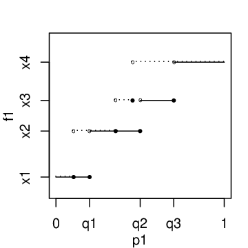
See Figure 1. For $j=1,\ldots,m$, define $\hat{p}_{j}=n^{-1}\sum_{i=1}^{n}\mathbbm{1}_{\{X_{i}=x_{j}\}}$ to be the empirical proportion of the sample taking the value $x_{j}$. Let $\epsilon=\min_{j}p_{j}/3$, write $\hat{q}_{j}=\hat{p}_{1}+\ldots+\hat{p}_{j}$, and define the event

Observe that, by the Dvoretsky–Keifer–Wolfowitz inequality (Massart 1990),

Thus, since $|\hat{F}_{n}^{-1}(p)-F^{-1}(p)|\leq x_{m}-x_{1}$,

as $n\rightarrow\infty$. On the other hand,

But $\bigl(n^{1/2}(\hat{q}_{1}-q_{1}),\ldots,n^{1/2}(\hat{q}_{m}-q_{m})\bigr)\stackrel{{\scriptstyle d}}{{\rightarrow}}N_{m}(0,\Sigma)$, where the asymptotic covariance matrix $\Sigma$ has entries $\Sigma_{ij}=q_{i}(1-q_{j})$, for $1\leq i\leq j\leq m$. So by the continuous mapping theorem,

as $n\rightarrow\infty$. Hence

as $n\rightarrow\infty$.        

Theorems 2.4 and 2.6 extend to the case of general $d_{r}$. Note the rates below coincide only when $r=1$, a case studied by del Barrio et al. 1999b.

Proof The proof of part $(a)$ follows that of Theorem 2.4, the only difference being that the function $h_{1}$ should in this case be defined by

Part $(b)$ mirrors the proof of Theorem 2.6, noting that in general,

where the event $A$ was defined in the proof of Theorem 2.6.        

In Section 2, we saw the importance of Conditions 1 and 2 concerning the tail behaviour of the distribution function $F$ in determining the rate of convergence to zero of $d_{2}(\hat{F}_{n},F)$. We now study the nature of these conditions in greater detail, using the notion of the hazard function.

The following theorem is the main result of this section, showing the redundancy of Condition 1. Its proof is deferred until after Lemma 3.4.

Let $X_{t}$ denote a random variable distributed as $X|X>t$, and consider ${\rm{Var\;}}X_{t}$ (we set ${\rm{Var\;}}X_{t}=0$ if $\mathbb{P}(X>t)=0$). For example, if $X$ is an exponential random variable, then $X_{t}\sim X+t$, and we have ${\rm{Var\;}}X_{t}={\rm{Var\;}}X$. In general, this tail variance is closely related to the hazard function, as shown by the following lemma.

Proof

(a) Proof of the lower bound. Define the function

Note that the density of $X_{t}$ for $x\geq t$ is $f(x)/\bar{F}(t)$, which is at most $k(t)$. By comparison with the $U[t,t+1/c]$ distribution, we see that if a random variable has density bounded above by $c$, then its variance is at least $1/(12c^{2})$, so ${\rm{Var\;}}X_{t}\geq 1/\bigl(12k(t)^{2}\bigr)$. Moreover, if $x\geq t$, then $f(x)/\bar{F}(t)\leq f(x)/\bar{F}(x)$, from which we deduce that $k(t)\leq\sup_{x\geq t}h(x)$.

(b) Proof of the upper bound. In fact, we establish the stronger conclusion that

We use arguments based on those which establish Poincaré inequalities, in Borovkov and Utev 1984 and Sysoeva 1965. The simplest possible case of the main theorem of Sysoeva 1965 gives a Hardy inequality, that if $G$ is a differentiable function with $G(t)=0$, then

where $g(x)=G^{\prime}(x)$, provided the integrals exist.

[For the sake of completeness, note that Equation (3) can be proved as follows. Integration by parts gives that

by Cauchy-Schwarz.] Hence, from Equation (3),

and choosing $G(x)=x-t$, Equation (2) follows.        

This shows that if $h(t)$ is bounded away from zero for large $|t|$, then ${\rm{Var\;}}X_{t}<\infty$. This is the case for the normal distribution, where the Mills ratio (Shorack and Wellner, 1986, p. 850) gives that $h(t)\geq|t|$ for all $t$. On the other hand, if $h(t)\rightarrow 0$ as $|t|\rightarrow\infty$, then ${\rm{Var\;}}X_{t}\rightarrow\infty$, as for the log-normal distribution, where $h(t)\sim t^{-1}\log t$ as $t\rightarrow\infty$. Finally we remark that other tail variance behaviour is possible, in the case where $\liminf_{t\rightarrow\infty}h(t)<\limsup_{t\rightarrow\infty}h(t)$.

As the example of the log-normal might suggest, results from reliability theory provide a link between the hazard function and the finiteness of the moment generating function in a neighbourhood of the origin.

Proof We prove the result for the right-hand tail. Observe that for $x\geq t$,

which can be seen by differentiating both sides with respect to $x$. Thus

Now the right-hand side of Equation (4) is bounded above by $e^{-cx}$, which is enough to guarantee that the moment generating function is finite for $\theta\in[0,c)$.        

Lemma 3.4 shows that if a random variable $X$ has a moment generating function which is infinite other than at the origin, then there exists a sequence $(x_{n})$ tending to infinity such that $\lim_{n\rightarrow\infty}h(x_{n})=0$. If, further, $X$ has a decreasing hazard function then we deduce that $\lim_{x\rightarrow\infty}h(x)=0$, and hence by Lemma 3.3, that $\lim_{t\rightarrow\infty}{\rm{Var\;}}X_{t}=\infty$.

We are now in a position to prove Theorem 3.2.

Proof of Theorem 3.2 We have

The second term tends to zero by Equation (2). If $\xi_{1}<\infty$, then the first term clearly converges in probability to zero. On the other hand, if $\xi_{1}=\infty$, then the assumed hypothesis on the hazard function combined with Equation (4) imply that for any $t>0$,

These are is precisely the conditions under which Galambos 1978, Theorem 4.1.2, proves convergence in probability of $X_{(n)}-\xi_{(n-1)/n}$ to zero. This completes the first part of the proof.

Note that Condition 2 can be restated in terms of the hazard function; that is, by considering the regions $x\in[\xi_{1/2},\infty)$ and $x\in(-\infty,\xi_{1/2})$ separately, we see that Condition 2 holds if and only if

Finiteness of this integral implies that $h(x)\rightarrow\infty$ as $|x|\rightarrow\infty$, and so by the argument above, Condition 1 holds.        

Note for the normal distribution that $h(x)\rightarrow\infty$, but, again by the Mills ratio,

Thus Condition 1 holds (implying Proposition 1 of del Barrio et al. 1999), but not Condition 2.

Finally in this section, we give a partial converse to Theorem 2.5.

Proof For $i=1,\ldots,n$, let $a_{i}=n\int_{(i-1)/n}^{i/n}F^{-1}(p)\,dp$. We decompose $nd_{2}^{2}(\hat{F}_{n},F)$ into a random and deterministic part as follows:

Ignoring the random part, the result is immediate.        

The bootstrap was introduced into Statistics in the landmark paper of Efron 1979, and gives a very general technique for approximating the distributions of roots (i.e. functions of the sample and parameters of the underlying population) of interest. The key idea for its use in practice is that of resampling; given a sample $X_{1},\ldots,X_{n}$, we draw a further sample $X_{1}^{*},\ldots,X_{n}^{*}$ uniformly at random with replacement from the original sample, and perform our calculations based on this resample. The opportunity to repeat this resampling procedure enables the practitioner to mimic drawing additional samples from the original population.

Historically, one of the great early triumphs in the analysis the bootstrap was the paper of Singh 1981. One of his main results was to show that the bootstrap distribution of a normalised sample mean converges to its true sampling distribution at rate $O(n^{-1})$, provided the underlying population is non-lattice, and sufficiently many moments exist. This improves on the $O(n^{-1/2})$ convergence rate of its natural competitor, namely normal approximation. Singh’s theorem was stated in terms of the supremum distance between the respective distribution functions. The Mallows metric was first considered in the context of the bootstrap by Bickel and Freedman 1981.

Recall that $X_{1},\ldots,X_{n}$ are independent random variables, each with distribution function $F$ with mean $\mu$ and finite variance $\sigma^{2}>0$, that $\hat{F}_{n}$ is the empirical distribution function of the sample and that $\bar{X}_{n}=n^{-1}\sum_{i=1}^{n}X_{i}$ is the sample mean. A standard procedure for constructing confidence intervals for $\mu$ is to invert a probability statement concerning a root such as $n^{1/2}(\bar{X}_{n}-\mu)$, whose sampling distribution under $F$ we denote by $H_{n}(F)$. Conditional on $X_{1},\ldots,X_{n}$, let $X_{1}^{*},\ldots,X_{n}^{*}$ be a resample; that is, an independent and identically distributed sample drawn from $\hat{F}_{n}$.

The nonparametric bootstrap estimates the sampling distribution of $n^{1/2}(\bar{X}_{n}-\mu)$ by that of $n^{1/2}(\bar{X}_{n}^{*}-\bar{X}_{n})$, where $\bar{X}_{n}^{*}=n^{-1}\sum_{i=1}^{n}X_{i}^{*}$. In other words, conditional on $X_{1},\ldots,X_{n}$, we approximate $H_{n}(F)$ by $H_{n}(\hat{F}_{n})$. The properties of the Mallows distance $d_{2}$ make it suitable for studying the performance of the bootstrap approximation in this context. The calculation below follows Shao and Tu 1995, and uses results proved in Bickel and Freedman 1981.

Thus, in particular, the distance between the distribution of the root of interest, $H_{n}(F)$, and its bootstrap approximation, $H_{n}(\hat{F}_{n})$, is stochastically dominated by the distance between the true and empirical distributions. The first inequality and the conditions under which we obtain equality are studied in Johnson and Samworth 2004.

Having studied the upper bound $d_{2}(\hat{F}_{n},F)$ in previous sections, our final result gives a lower bound on the rate of convergence of $d_{2}\bigl(H_{n}(\hat{F}_{n}),H_{n}(F)\bigr)$. Observe in particular that if the hypotheses of Theorem 2.4 and Proposition 4.1 are both satisfied, then the rates of convergence of the two bounds are identical.

Proof For any $r\geq 1$ and $F_{X},F_{Y}\in\mathcal{F}_{r}$, there exist random variables $(X,Y)$ having marginal distribution functions $F_{X}$ and $F_{Y}$ respectively, and such that

References

- Bickel and Freedman (1981) Bickel, P. J. and Freedman, D. A. (1981), Some asymptotic theory for the bootstrap, Ann. Statist., 9, 1196–1217.
- Billingsley (1999) Billingsley, P. (1999), Convergence of Probability Measures, Second ed., Wiley, New York.
- Borovkov and Utev (1984) Borovkov, A. and Utev, S. (1984), On an inequality and a related characterisation of the normal distribution, Theor. Probab. Appl., 28, 219–228.
- Chibisov (1965) Chibisov, D. M. (1965), An investigation of the asymptotic power of the tests of fit, Theor. Probab. Appl., 10, 421–437.
- Csörgő and Horváth (1990) Csörgő, M. and Horváth, L. (1990), On the distributions of norms of weighted quantile processes, Ann. Inst. Henri Poincaré, 26, 65–90.
- del Barrio et al. (1999) del Barrio, E., Cuesta-Albertos, J. A., Matrán, C. and Rodríguez-Rodríguez, J. M. (1999), Tests of goodness of fit based on the -Wasserstein distance, Ann. Statist., 27, 1230–1239.
- del Barrio et al. (1999b) del Barrio, E., Giné, E. and Matrán, C. (1999b), Central limit theorems for the Wasserstein distance between the empirical and the true distributions, Ann. Probab., 27, 1009–1071.
- del Barrio et al. (2000) del Barrio, E., Cuesta-Albertos, J. A., Matrán, C. (2000), Contributions of empirical and quantile processes to the asymptotic theory of goodness-of-fit tests, Trabajos Investigación Oper., 9, 1–96.
- Efron (1979) Efron, B. (1979), Bootstrap methods: another look at the jackknife, Ann. Statist., 7, 1–26.
- Fisz (1963) Fisz, M. (1963), Probability Theory and Mathematical Statistics, Third ed., Wiley, New York.
- Galambos (1978) Galambos, J. (1978), The Asymptotic Theory of Extreme Order Statistics, Wiley, New York.
- Johnson and Samworth (2004) Johnson, O. T. and Samworth, R. J. (2004), Central limit theorem and convergence to stable laws in Mallows distance, submitted to Bernoulli and available at tex-arkiv paper no. math.PR/0406218.
- Loève (1977) Loève, M. (1977), Probability Theory I, Fourth Ed., Springer-Verlag, New York.
- Major (1978) Major, P. (1978), On the invariance principle for sums of independent, identically distributed random variables, J. Mult. Anal., 8, 487–501.
- Massart (1990) Massart, P. (1990), The tight constant in the Dvoretsky–Keifer–Wolfowitz inequality, Ann. Probab., 18, 1269–1283.
- Rachev (1984) Rachev, S. T. (1984), The Monge-Kantorovich problem on mass transfer and its applications in stochastics, Theor. Probab. Appl., 29, 647–676.
- Serfling (1980) Serfling, R. J. (1980), Approximation Theorems of Mathematical Statistics, Wiley, New York.
- Shao and Tu (1995) Shao, J. and Tu, D. (1995), The Jackknife and Bootstrap, Springer-Verlag, New York.
- Shorack and Wellner (1986) Shorack, G. R. and Wellner, J. A. (1986), Empirical Processes with Applications to Statistics, Wiley, New York.
- Singh (1981) Singh, K. (1981), On the asymptotic validity of Efron’s bootstrap, Ann. Statist., 9, 1187–1195.
- Sysoeva (1965) Sysoeva, F. A. (1965), Generalization of a certain Hardy inequality, Izv. Vysš. Učebn. Zaved. Matematika, 49, 140–143.