The dynamics of Pythagorean triples
Abstract
We construct a piecewise onto 3-to-1 dynamical system on the positive quadrant of the unit circle, such that for rational points (which correspond to normalized Primitive Pythagorean Triples), the associated ternary expansion is finite, and is equal to the address of the PPT on Barning’s [9] ternary tree of PPTs, while irrational points have infinite expansions. The dynamical system is conjugate to a modified Euclidean algorithm. The invariant measure is identified, and the system is shown to be conservative and ergodic. We also show, based on a result of Aaronson and Denker [2], that the dynamical system can be obtained as a factor map of a cross-section of the geodesic flow on a quotient space of the hyperbolic plane by the group , a free subgroup of the modular group with two generators.
1 Introduction
The starting point of this paper is a theorem, attributed to Barning [9], on the structure of the set of Primitive Pythagorean Triples, or PPTs. Recall that a PPT is a triple of integers, with and
| (1) |
Clearly, if is a PPT, then one of must be odd, and the other even. Barning [9], and later independently several others [7, 11, 12, 14, 15, 17, 20] (see also [19]), showed:
Theorem 1.
Define the matrices
| (2) |
Any PPT with odd and even has a unique representation as the matrix product
| (3) |
for some , . Any PPT with even and odd has a unique representation as
| (4) |
for some , . Any triple of one of the forms (3), (4) is a PPT.
In some of the papers where this was discussed, the theorem has been described as placing the PPTs with odd and even on the nodes of an infinite rooted ternary tree, with the root representing the “basic” triple , and where each triple has three children, representing the multiplication of the triple (considered as a column vector) by the three matrices . In this paper, we consider a slightly different outlook. We think of the sequence in (3), (4) as an expansion corresponding to the triple , over the ternary alphabet . We call the ’s the digits of the expansion. To distinguish between PPTs with odd, even and those with even, odd, we affix to the expansion a final digit , which can take the values ( odd, even) or ( even, odd). So we have a 1-1 correspondence
Several questions now come to mind:
- •
Is there a simple way to compute the expansion of a PPT? (Yes – this is contained in the proof of Theorem 1.)
- •
As is easy to see and has been known since ancient times, the mapping gives a 1-1 correspondence between the set of PPTs and the rational points on the positive quadrant of the unit circle. Are the digits in the expansion piecewise continuous functions on the quadrant? (Yes.) Can one define a ternary expansion for irrational points? (Yes.)
- •
Can interesting things be said about the expansion of a random PPT, chosen from some natural model for random PPTs, say by choosing uniformly at random from all PPTs with and letting ? (Yes.)
- •
Do these questions lead to interesting mathematics? (Yes – they lead to a dynamical system on with interesting properties.)
It is the goal of this paper to answer these questions. The basic observation is that it is in many ways preferable to deal with points on the positive quadrant of the unit circle, instead of with PPTs. In the proof of Theorem 1, we shall see that there is a simple transformation (a piecewise linear mapping) that takes a PPT to the PPT that corresponds to its parent on the ternary tree, i.e., if has expansion then has expansion . A standard trick in dynamical systems is to rescale such transformations, discarding information that is irrelevant for the continuing application of the transformation; this is done, for example, when rescaling the Euclidean algorithm mapping to obtain the continued fraction transformation . When we apply this idea to our case, we obtain the following result.
Theorem 2.
Let
Define the transformation by
Define by
Then:
- (i)
- (ii)
If is an irrational point, then for all , and the sequence
defines an infinite expansion for over the alphabet , with the property that it does not terminate with an infinite succession of ’s or with an infinite succession of ’s.
- (iii)
Any sequence over the alphabet which does not terminate with an infinite succession of ’s or an infinite succession of ’s determines a unique (irrational) point such that .
Examples.
Here are some examples of points in and their expansions. If is an expansion (finite or infinite), we denote by the point which has the given sequence as its expansion.
(see section 5)
(this is meant as an example of a “typical” expansion – see section 4)
where and are sequences A046727 and A001653, respectively, in The On-Line Encyclopedia of Integer Sequences [24].
After constructing the dynamical system associated with the ternary expansion, the next step is to study its properties. What does the expansion of a typical point look like? To a trained eye, the answer is contained in the following theorem.
Theorem 3.
Let denote arc length on the unit circle. The dynamical system possesses an infinite invariant measure , given by
With the measure , the system is a conservative and ergodic infinite measure-preserving system.
The invariant measure encodes all the information about the statistical regularity of expansions of “typical” points. In section 4 we shall state more explicitly some of the number-theoretic consequences of Theorem 3.
Recall ([13], Theorem 225) that the general parametric solution of the equation (1) with coprime, odd and even is given by
| (5) |
where have opposite parity, , and . A roughly equivalent statement is that the map
maps the extended real line injectively onto the unit circle, and maps the rational numbers, together with the point at infinity, onto the rational points of the circle. Note also that the interval is mapped onto the positive quadrant . It is thus natural, in trying to understand the behavior of the dynamical system , to conjugate it by the mapping , to obtain a new dynamical system on . This leads to the following result (the precise meaning of the last statement in the theorem will be explained later):
Theorem 4.
is conjugate, by the mapping , to the measure preserving system , where
The mapping is the scaling of a modified slow (subtractive) Euclidean algorithm.

There has been some interest in obtaining natural dynamical systems appearing in number theory as factors of certain cross sections of the geodesic flow on quotients of the hyperbolic plane by a discrete subgroup of its isometry group. This has been done by Adler and Flatto [4, 6] and by Series [22] for the continued fraction transformation, and by Adler and Flatto [5] for Rényi’s backward continued fraction map (see also [3, 23]). In both of these cases, the underlying surface was the modular surface, which is the quotient of the hyperbolic plane by the modular group . Representing a system as a factor of a cross-section of a geodesic flow enables one to derive mechanically (without guessing) an expression for the invariant density, and to deduce various properties of the system. Series ([23], Problem 5.25(i)) posed the general problem of replicating this idea for other number- and group-theoretical dynamical systems.
It turns out that the map also admits such a representation. Aaronson and Denker [2] studied a certain cross-section of the geodesic flow on a different quotient of the hyperbolic plane, which is the quotient by the congruence subgroup of the modular group, a free group with two generators. They obtained the map as a factor of that cross section, and used this to derive results on the asymptotic behavior of the Poincaré series of the group of deck transformations of . Since in their paper the motivation was completely different from ours, and the connection to the map was not known, we find it worthwhile to include here a version of their result.
Theorem 5.
Let be the upper half-plane model of the hyperbolic plane, with the associated geodesic flow , where is the unit tangent bundle of . Define the group of isometries of
and let be the quotient space of by , which has a fundamental domain
Let be the quotient map. Let be the geodesic flow on . Let ,
and let , be the natural section of corresponding to the fundamental domain of all inward-pointing vectors on the boundary of . Let be the section- or first-return map of the geodesic flow, namely
where
Then the section map admits the map as a factor. That is, there exists an (explicit) function such that .
Theorem 5 is an immediate consequence of Aaronson and Denker’s result ([2], section 4) and Theorem 4. To describe explicitly the factor map , define . Then, in the notation of their paper,
with the “juicy” parts being our map and and the map , which assigns to a tangent vector the hitting point on the real axis of the geodesic emanating from the lifting of the tangent vector to . For more details consult [2].
The congruence subgroup also appears in the paper by Alperin [7], which discusses the ternary tree of PPTs.
In the next section, we reprove Theorem 1, and show how the linear mappings involved in the construction of the ternary tree of PPTs can be scaled down to produce the transformation . This will result in a proof of Theorem 2. In section 3, we prove Theorem 4 and discuss the connection to modified Euclidean algorithms. The ergodic properties of the system will be derived, using standard techniques of infinite ergodic theory, proving Theorem 3. In section 4 we discuss applications to the statistics of expansions of random points on and random PPTs. Section 5 has some remarks on points with special expansions.
2 Construction of the dynamical system
2.1 The piecewise linear transformation
First, we recall the ideas involved in the proof of Theorem 1. We follow the elegant exposition of [18].
We shall consider solutions of (1) with , and . Define
| PPT | ||||
| the set of PPTs, and | ||||
| SPPT | ||||
The basic observation is that the equation (1) has three symmetries. Two of them are the obvious symmetries , (we ignore the symmetry , since we are only considering solutions with ). The third symmetry is not so obvious, but becomes obvious when the correct change of variables is applied. Define new variables by
In the new variables, (1) becomes
| (7) |
There is therefore a third natural involution on the set SPPT of solutions of (1), given in coordinates by . So, starting from a solution with associated variables and setting , we arrive at a new solution given by
or in matrix notation
The matrix is an involution, i.e. . It is easy to see that are also coprime, and
So maps SPPT to itself. has the fixed points and . We claim that . Indeed, this simply means that if , then at least one of is negative, or in other words that . Assume for concreteness that , then if , where , or equivalently if
| (8) |
The point lies on the arc , and one checks easily that there is an equality at one end of the arc, and a strict inequality at the other end . So (8) holds.
Having shown that if , then is a signed PPT with one of negative, we can forget about the signs of and obtain a new triple . is strictly less than , since and on PPT. The new triple will be a PPT, except when or , in which case will equal or , respectively. If is a PPT, there are precisely three PPTs leading to it via this procedure – corresponding to the three possible sign patterns (we ruled out ) – and they can easily be recovered, as follows: If , then
(with as in (2)). Similarly we get
We are now ready to prove Theorem 1. First, from the above discussion it follows that take PPTs to PPTs with a strictly larger third coordinate. In particular, any triple of one of the forms (3), (4) is a PPT. Next, for define
The above discussion can be summarized by the equations
| (10) |
Let with odd and even. It is easy to see that preserve the parity of , so cannot have a representation (4). We claim that it satisfies (3) with , , and that this representation is unique. The proof is by induction on . The claim holds for the basic triple , because increase the third coordinate. Assume that it holds for all odd-even PPTs with third coordinate . Then in particular this is true for , since we know that . So we may write
with , . We have
where we denote . Therefore, by (10),
which is our claimed representation. Uniqueness follows immediately by noting that by (10), is determined by the sign pattern of , and continuing by induction. Theorem 1 is proved.
2.2 Scaling the transformation
It is now easy to rescale the transformation to obtain a transformation from to its closure. If is a rational point of , which corresponds to the PPT , then the triple corresponds to the point
in . This precisely accounts for our definition of in Theorem 2. To explain why the function is the correct rescaling of , observe, for example, that iff
which some inspection reveals to hold exactly on the (open) circular arc connecting the point with the point . This corresponds to the condition in the definition of . Similarly, it can be checked that if lies on the circular arc between and , and if lies on the circular arc between and . These arcs form the generating partition of the ternary expansion – see Figure 2.
Figure 3 shows the graph of the map obtained by parametrizing the quadrant in terms of the angle (multiplied by , to obtain a map on the interval ). As Theorem 4 may imply, this is not the best parametrization, but it gives a good graphical illustration of the behavior of the mapping . Note that, contrary to appearance, the map is not linear on the middle interval!
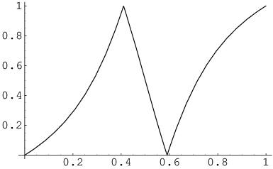
We have proved part (i) of Theorem 2. For part (ii), observe that all the iterates of an irrational point under remain irrational, since is defined by piecewise rational functions with integer coefficients which are invertible (so as before, given , we can recover from by a rational function with integer coefficients, hence if is rational, so is ). For to be in , we must have or , and this cannot happen for an irrational point. Therefore is defined for all , as claimed. The resulting sequence of digits cannot terminate with an infinite succession of 1’s. Indeed, on the first interval of the generating partition of the mapping (Figure 3) it is easy to verify that is increasing and satisfies . Therefore if is some point on this interval, then the sequence of iterates satisfies and therefore must eventually leave this interval (so the corresponding succession of 1’s in the expansion will terminate). A symmetrical argument applies for the third interval of the generating partition, implying that no infinite expansion terminates with an infinite succession of 3’s, and part (ii) is proved.
Turn to the final part (iii) of Theorem 2. Again we use the mapping in Figure 3. Let , , be the intervals of the generating partition of . Given an infinite expansion that does not terminate with an infinite succession of ’s or an infinite succession of ’s, we must show that there is a unique number such that for all .
Consider, for any , the cylinder set
is a decreasing sequence of non-empty open intervals. By compactness, the intersection of their closures contains at least one point . The condition on the sequence implies that is in fact in the intersection of the open intervals; otherwise, is an endpoint, say of , but that would imply that for all or for all .
We have shown existence of a number with a prescribed expansion. But uniqueness also follows, since, as Figure 3 shows, any appearance of a “2” digit, or a non-1 digit following a succession of 1’s, or a non-3 digit following a succession of 3’s, entails a shrinkage of the corresponding set by at least a constant factor bounded away from 1. So the diameter of the ’s goes to 0, and their intersection contains at most one point. Theorem 2 is proved.
(Here is another argument demonstrating uniqueness: any two irrational points on are separated by a rational point; after a finite number of applications of , the rational point will be mapped to or to , and the images of the two irrational points will be contained in different elements of the generating partition, implying a different first digit in their expansions.)
3 The modified Euclidean algorithm
3.1 Some computations
The inverse function of is easily computed to be
Using this, a routine computation, which we omit, shows that indeed
We show that the measure is -invariant. If , the invariant density must satisfy
| (11) |
The inverse branches of are given by
| (12) |
for which
So (11) reduces to
| (13) |
Check directly that satisfies (13).
To complete the proof of Theorem 4, we need to verify that is the push-forward of the measure under . Denote
Compute:
as claimed.
Note that this also proves that is -invariant. This fact could be checked directly, of course.
3.2 Interpretation as a Euclidean algorithm
The ordinary Euclidean algorithm takes a pair of positive integers with and returns the pair . After a finite number of iterations of this mapping, will be equal to and will be equal to the g.c.d. of the original pair.
Many variants of this algorithm have been analyzed, where various alternatives to simple division with remainder are used. The study of such algorithms, related of course to continued fraction variants, is a huge subject which it is beyond the scope of this paper to describe. See [21]; sections 4.5.2-4.5.3 in [16] and the references there; and [8] for some more recent developments.
The standard Euclidean algorithm has a more ancient version, known as the slow, or subtractive Euclidean algorithm, where subtraction is used instead of division, so are mapped to . Clearly the standard algorithm is nothing more than a speeding-up of this algorithm. One may scale by always replacing by 1 and by the ratio . This leads to the interval map ,
We now observe that the map is itself the scaling of a modified algorithm, defined by the mapping
Here is a sample execution sequence of this algorithm:
This algorithm can be used to compute g.c.d.’s, just like its famous kin: The last output which differs from the one preceding it is of either the form or , where is the g.c.d. of the two original integers.
3.3 Ergodic properties of
To prove Theorem 3, we study the somewhat simpler measure preserving system . Since this is now represented as an interval map, we can use standard techniques of ergodic theory.
Define . Define the set . An alternative description for is as the cylinder set
By Theorem 2(ii), for any irrational , for some . In other words,
This implies that is conservative, by [1], Theorem 1.1.7.
To prove that is ergodic, we pass to the induced system , where
By the explicit description of given in [2], p. 16, it follows ([2], Lemma 5.2) that is a topologically mixing Markov map which is uniformly expanding with bounded distortion, i.e., satisfies
Therefore ([1], Theorem 4.4.7) it is exact, and in particular it is ergodic. It follows ([1], Proposition 1.5.2(2)) that is itself ergodic. This completes the proof of Theorem 3.
4 Expansions of random -points and random PPTs
4.1 Random points on
The invariant measure becomes infinite near the two ends of the quadrant . This means that in a typical expansion, the digits “1” and “3” will occur infinitely more often than the middle digit “2”. However, for any two digit sequences, even ones that contain the digits “1” and “3”, we can ask about their relative density of occurence in the expansion of typical points.
Theorem 6.
Let be the intervals of the generating partition of . For , define
with as in (12). Let . For almost every , the limit
exists and is equal to .
Proof.
This is an immediate consequence of Hopf’s ergodic theorem, applied to the two indicator functions of the cylinder sets and .
Example.
An easy computation gives
Therefore, in a typical expansion, when a run of consecutive 1’s breaks, the next digit will be a “2” with probability , or a “3” with probability .
4.2 Random PPTs
PPTs have finite expansions and form a subset of of measure 0. So, as the analogous studies of continued fraction expansions of rational numbers (a.k.a. analysis of the Euclidean algorithm) have shown, analyzing their behavior can be significantly more difficult than the behavior of expansions of random points on . We outline here a technique for easily deducing some of the properties of the expansion by relating the discrete model to the continuous one. We mention some open problems which may be approachable using more sophisticated methods such as those used in [8], and which we hope to address at a later date.
Our model for random PPTs will be the discrete probability space
equipped with the uniform probability measure . Analogous results can easily be formulated, using the same ideas presented here, for other natural models, e.g., a uniform choice of with .
We discuss the distribution of the individual digits in the expansion. Let be the uniform arc-length measure on , normalized as a probability measure. That is, . We need the following simple lemma.
Lemma 7.
Under the measure , the random vector converges in distribution to .
Proof.
Observe the following fact from elementary number theory: the coprime pairs such that are of opposite parity have a local density of in the lattice , in the following sense: for any bounded open set , we have
| (15) |
First, this is true when is a rectangle . To prove this, define for ,
Let be the coefficients of the Dirichlet series
Then the left-hand side of (15) is equal to
Since clearly (for odd), this is easily seen to be as , where
proving our claim.
It follows, by taking unions and differences, that (15) is true for any finite union of rectangles with sides parallel to the coordinate axes, and therefore by approximation for any bounded and open .
This is exactly the claim of the Lemma.
Define the Perron-Frobenius operator of as the operator ,
is also known as the transfer operator corresponding to . It has the property that if the random vector on has distribution , then has distribution . We skip the simple computation that verifies this claim.
Theorem 8.
Under , the distribution of , the -th digit in the expansion of a random PPT , converges to the distribution of under the measure
where is the constant function .
Proof.
This is immediate from Lemma 7 and the definition of .
Theorem 8 answers the question of the limiting distribution as of the digits in the expansion of a random PPT; however, it does not give good asymptotic information on the behavior of these distributions as . In fact, this is not a very interesting question: since the invariant measure is infinite, the density will become for large more and more concentrated around the singular points and (it is possible to make this statement more precise, but we do not pursue this slightly technical issue here).
Here’s one way to amend the situation in a way that enables formulating interesting quantitative statements concerning the distribution of the digits, which we mention briefly without going into detail: replace the expansion by a new expansion , by dividing the into blocks consisting of 1’s and 3’s and terminating with a 2; so for instance, the expansion will be replaced by . The new expansion corresponds to the induced transformation , where is the middle arc in the generating partition. Cylinder sets of can be easily computed. The invariant measure is the restriction , a finite measure, so normalize it to be a probability measure. is easily shown to be exact as in section 3.3. A theorem analogous to Theorem 8 above can be proved, to the effect that the -th digit in the “new” expansion of a random PPT converges in distribution to the distribution of (the first “new” digit) under the measure whose density with respect to is the -th iterate of the Perron-Frobenius operator of applied to the constant function . Since is mixing, these densities will actually converge to the invariant density. So after each occurence of a “2” in the original expansion, there are well-defined statistics for the sequence of digits that follows up to the next “2”.
We conclude with some open problems: study the expectation, the variance and the limiting distribution of the length of the expansion of a random element of , as . Generalize to arbitrary cost-functions, as in [8].
5 Some special expansions
From a number-theoretic standpoint, it is interesting to study points on with special expansions. As the examples in section 1 show, simple periodic expansions seem to correspond to simple quadratic points on . It is easy to see that any eventually-periodic expansion corresponds to the image under of a quadratic irrational. Do all quadratic irrationals have eventually periodic expansions?
We also found empirically the expansions
where means a succession of 1’s. The first equation can be proved by observing that , and that the approximations
( as in (12)) have the continued fraction expansions
Thus our expansion reduces to the known ([24], sequence A019425) infinite continued fraction expansion
The second equation is proved similarly. It is interesting to wonder whether other “nice” expansions exist for simple points on .
Acknowledgements
Thanks to Jon Aaronson and to Boaz Klartag for helpful discussions.
References
- [1] J. Aaronson, An Introduction to Infinite Ergodic Theory. Mathematical Surveys and Monographs 50, Amer. Math. Soc, Providence, RI, 1997.
- [2] J. Aaronson, M. Denker, The Poincaré series of . Ergodic Theory Dynam. Systems 19 (1999), 1–20.
- [3] R. L. Adler, Geodesic flows, interval maps, and symbolic dynamics. In: Ergodic Theory, Symbolic Dynamics and Hyperbolic Spaces, 93–123. Oxford University Press, Oxford, 1991.
- [4] R. L. Adler, L. Flatto, Cross section maps for geodesic flows I (the modular surface). In: Ergodic theory and dynamical systems, vol. 2 (College Park, Maryland 1979-1980), 103–161. Progr. Math., 21, Birkhäuser, Boston, Mass., 1982.
- [5] R. L. Adler, L. Flatto, The backward continued fraction map and geodesic flow. Ergodic Theory Dynam. Systems 4 (1984), 487–492.
- [6] R. L. Adler, L. Flatto, Cross section map for the geodesic flow on the modular surface. In: Conference in modern analysis and probability (New Haven, Conn., 1982), 9–24. Contemp. Math., 26, Amer. Math. Soc., Providence, RI, 1984.
- [7] R. Alperin, The Modular tree of Pythagoras. Preprint, 2000. http://www.arxiv.org/abs/math.HO/0010281.
- [8] V. Baladi, B. Valleé, Euclidean algorithms are Gaussian. Preprint, 2003. http://arxiv.org/abs/cs.DS/0307062
- [9] F. J. M. Barning, On Pythagorean and quasi-Pythagorean triangles and a generation process with the help of unimodular matrices. (Dutch) Math. Centrum Amsterdam Afd. Zuivere Wisk., ZW-011 (1963).
- [10] P. Billingsley, Ergodic Theory and Information. John Wiley & Sons, New York-London-Sydney 1965.
- [11] J. Gollnick, H. Scheid, J. Zöllner, Rekursive Erzeugung der primitiven pythagoreischen Tripel. (German) Math. Semesterber. 39 (1992), 85–88.
- [12] A. Hall, Genealogy of Pythagorean triads. Math. Gazette 54:390 (1970), 377–379.
- [13] G. H. Hardy, E. M. Wright, An Introduction to the Theory of Numbers, 5th ed. Oxford University Press, Oxford, 1985.
- [14] J. Jaeger, Pythagorean number sets. (Danish.) Nordisk Mat. Tidskr. 24 (1976), 56–60, 75.
- [15] A. R. Kanga, The family tree of Pythagorean triples. Bull. Inst. Math. Appl. 26 (1990), 15–17.
- [16] D. E. Knuth, The Art of Computer Programming, vol. 2: Seminumerical Algorithms, 3rd. ed. Addison-Wesley, 1998.
- [17] E. Kristensen, Pythagorean number sets and orthonormal matrices. (Danish) Nordisk Mat. Tidskr. 24 (1976), 111–122, 135.
- [18]
A. Lönnemo,
The trinary tree underlying primitive pythagorean triples.
In: Cut the Knot, Interactive Mathematics Miscellany and
Puzzles. Alex Bogomolny (Ed.),
http://www.cut-the-knot.org/pythagoras/PT_matrix.shtml. - [19] D. McCullough, Height and excess of Pythagorean triples. Preprint.
- [20] P. Préau, Un graphe ternaire associé à l’équation . C. R. Acad. Sci. Paris Ser. I Math. 319 (1994), 665–668.
- [21] F. Schweiger, Ergodic Theory of Fibred Systems and Metric Number Theory. Clarendon Press, Oxford, 1995.
- [22] C. Series, The modular surface and continued fractions. J. London Math. Soc. (2) 31 (1985), 69–80.
- [23] C. Series, Geometrical methods of symbolic coding. In: Ergodic Theory, Symbolic Dynamics and Hyperbolic Spaces, 125–151. Oxford University Press, Oxford, 1991.
- [24] N. J. A. Sloane, editor (2003), The On-Line Encyclopedia of Integer Sequences. http://www.research.att.com/ njas/sequences/.