Barvinok’s Rational Functions: Algorithms and Applications to Optimization, Statistics, and Algebra

Ruriko Yoshida

August 11, 2026

Ruriko Yoshida

B.A. (University of California at Berkeley) 2000

DISSERTATION

Submitted in partial satisfaction of the requirements for the degree of

DOCTOR OF PHILOSOPHY

MATHEMATICS

in the

OFFICE OF GRADUATE STUDIES

of the

UNIVERSITY OF CALIFORNIA

DAVIS

Approved:

Committee in Charge

2004

To Pete Camagna,

for his love and support.

ACKNOWLEDGEMENTS

First, I would like to thank my parents, Tasturou Yoshida and Chizuko Yoshida, in Japan for being patient with me.

Also I would like to thank my husband Pete Camagna for all support and for encouragement to write this thesis. He supported me emotionally and gave me great inspiration to create some algorithms. He has been always here for me no matter what happens.

I would like to thank Prof Jesús A. De Loera for all his help as my thesis advisor. He introduced me to Computational Algebra and Combinatorial generating functions in integer programming and Statistics. Without him, I would not know these interesting topics. He also motivated me to learn computer language C and C++, which I did not like when I was an undergraduate student. I really love to implement algorithms in C++ now and create interesting algorithms to apply Statistics and Combinatorial optimization. I really thank him for this. I also wish to thank my thesis committee, Roger Wets and Naoki Saito for taking their time to read this thesis.

I would also thank Raymond Hemmecke for useful conversations and encouragement to improve my thesis. He was like my big brother, looking after me and giving me great advice.

I would also like to thank Bernd Sturmfels. Bernd Sturmfels gave me much great advice for improving the LattE software, on which I was the head programmer. LattE is the only implementation to count the number of any rational convex polytope. Also when I was taking a phylogeny seminar from him in Berkeley, he gave me many great inspirations applying Algebraic algorithms to Biostatistics and Algebraic Statistics. Even though he is really busy, he looks after me and gives me great advises. He is my greatest inspiration for Mathematics.

Toward the end, Lior Pachter helped me on many aspects. I am so glad that I have an opportunity to work with him.

Finally I would like to thank all my best friends, Alice Stevens and Peter Huggins, for their encouragement and support to finish this thesis. Pete Camagna, Alice Stevens, and Peter Huggins are always here for me, every time I have problems and have been stressed out. Without them I would not have finished this thesis.

I am really lucky to have so many people who have been supportive.

This thesis was partially supported by NSF Grants DMS-0309694,and DMS-0073815.

Abstract

The main theme of this dissertation is the study of the lattice points in a rational convex polyhedron and their encoding in terms of Barvinok’s short rational functions. The first part of this thesis looks into theoretical applications of these rational functions to Optimization, Statistics, and Computational Algebra. The main theorem on Chapter 2 concerns the computation of the toric ideal $I_{A}$ of an integral $n\times d$ matrix $A$ . We encode the binomials belonging to the toric ideal $I_{A}$ associated with $A$ using Barvinok’s rational functions. If we fix $d$ and $n$ , this representation allows us to compute a universal Gröbner basis and the reduced Gröbner basis of the ideal $I_{A}$ , with respect to any term order, in polynomial time. We also derive a polynomial time algorithm for normal form computations which replaces in this new encoding the usual reductions of the division algorithm. Chapter 3 presents three ways to use Barvinok’s rational functions to solve Integer Programs: The $(A,b,c)$ -test set algorithm, the Barvinok’s binary search algorithm, and the digging algorithm.

The second part of the thesis is experimental and consists mainly of the software package LattE, the first implementation of Barvinok’s algorithm to compute short rational functions which encode the lattice points in a rational convex polytope. In Chapter 4 we report on experiments with families of well-known rational polytopes: multiway contingency tables, knapsack type problems, and rational polygons, and we present formulas for the Ehrhart quasi-polynomials of several hypersimplices and truncations of cubes. We also developed a new algorithm, the homogenized Barvinok’s algorithm to compute the generating function for a rational polytope. We showed that it runs in polynomial time in fixed dimension. With the homogenized Barvinok’s algorithm, we obtained new combinatorial formulas: the generating function for the number of $5\times 5$ magic squares and the generating function for the number of $3\times 3\times 3\times 3$ magic cubes as rational functions.

Chapter 1 Introduction

1.1 Basic notations and definitions

In this section, we will recall basic notations and definitions. Let $\{x_{1},x_{2},\dots,x_{m}\}$ be a finite set of points in $\mathbb{R}^{d}$ . A point

x=\sum_{i=1}^{m}\alpha_{i}x_{i},\mbox{ where }\sum_{i=1}^{m}\alpha_{i}=1\mbox{ and }\alpha_{i}\geq 0\mbox{ for }i=1,2,\dots,m

is called a convex combination of $x_{1},x_{2},\dots,x_{m}$ . Given two distinct points $x,\,y\in\mathbb{R}^{d}$ , the set $[x,y]=\{\alpha x+(1-\alpha)y:0\leq\alpha\leq 1\}$ of all convex combinations of $x$ and $y$ is called the interval with endpoints $x$ and $y$ . A set $C\subset\mathbb{R}^{d}$ is called convex, provided $[x,y]\subset C$ for any two $x,\,y\in C$ . For $C\subset\mathbb{R}^{d}$ , the set of all convex combinations of points from $C$ is called the convex hull of $C$ and denoted $\mbox{conv}(C)$ . Let $A_{1},A_{2},\dots,A_{n}\in\mathbb{R}^{d}$ and let $b_{1},b_{2},\dots,b_{n}\in\mathbb{R}$ . Then the set

P:=\{x\in\mathbb{R}^{d}:A_{i}\cdot x\leq b_{i}\mbox{ for }i=1,2,\dots,n\}

is called a polyhedron. The convex hull of a finite set of points in $\mathbb{R}^{d}$ is called a polytope and the Weyl-Minkowski Theorem says that a polytope is a bounded polyhedron (Schrijver 1986).

A finite set of points $\{x_{1},x_{2},\ldots,x_{k}\}\subseteq\mathbb{R}^{d}$ is affinely independent if $\forall\lambda_{j}\in\mathbb{R}$ , $\sum_{j=1}^{k}\lambda_{j}x_{j}=0,\sum_{j=1}^{k}\lambda_{j}=0$ $\Rightarrow$ $\lambda_{j}=0$ $\forall j=1,2,\ldots,k$ .

A $(d-1)$ dimensional affine set in $\mathbb{R}^{d}$ is called a hyperplane and every hyperplane can be represented as $\{x\in\mathbb{R}^{d}:ax=b$ , $a\in\mathbb{R}^{d}$ , $a\not=0$ , $b\in\mathbb{R}\}$ . $a$ is called a normal vector of this hyperplane.

Let $H:=\{x\in\mathbb{R}^{d}:h\cdot x\leq\beta\}$ , where $h\in\mathbb{R}^{d}$ , $h\not=0$ , and $\beta\in\mathbb{R}$ , be an affine half space. Then if $P\subset H$ and $P\cap\{x\in\mathbb{R}^{d}:h\cdot x=\beta\}\not=\emptyset$ , then $H$ is called a supporting hyperplane of $P$ . A subset $F$ of $P$ is called a face if $F=P$ or $F=P\cap H$ , where $H$ is a supporting hyperplane. If a face $F$ is minimal with respect to inclusion and $F$ contains only a point, then $F$ is called a vertex.

Let $V(P)$ be the set of all vertices of $P$ . If any points in $V(P)$ are in ${\mathbb{Z}}^{d}$ then $P$ is called an integral polyhedron. If any points in $V(P)$ are in ${\mathbb{Q}}^{d}$ then $P$ is called a rational polyhedron.

Now we will define our main tool, a generating function of a polyhedron. Let $P\subset\mathbb{R}^{d}$ be a polyhedron and let ${\mathbb{Z}}^{d}\subset\mathbb{R}^{d}$ be the integer lattice. For an integral point $m=(m_{1},m_{2},\dots,m_{d})\in{\mathbb{Z}}^{d}$ , we can write the monomial

z^{m}:=z^{m_{1}}_{1}z_{2}^{m_{2}}\dots z_{d}^{m_{d}}

in $d$ complex variables, $z_{1},z_{2},\dots,z_{d}$ . The generating function $f(P,z)$ of a polyhedron $P$ is the sum of monomials such that:

f(P,z)=\sum_{m\in P\cap{\mathbb{Z}}^{d}}z^{m}.

(1.1)

For example, consider the integral quadrilateral shown in Figure 1.1 with the vertices $V_{1}=(0,0)$ , $V_{2}=(5,0)$ , $V_{3}=(4,2)$ , and $V_{4}=(0,2)$ . Then we have the generating function $f(P,z)$ such that:

Refer to caption — Figure 1.1: An example for the generating function

$f(P,z)={z_{1}}^{5}+{z_{1}}^{4}z_{2}+{z_{1}}^{4}+{z_{1}}^{4}{z_{2}}^{2}+z_{2}{z_{1}}^{3}+{z_{1}}^{3}+{z_{1}}^{3}{z_{2}}^{2}+z_{2}{z_{1}}^{2}+{z_{1}}^{2}+{z_{1}}^{2}{z_{2}}^{2}+z_{1}z_{2}+z_{1}+z_{1}{z_{2}}^{2}+{z_{2}}^{2}+z_{2}+1$ .

One notices that the multivariate generating function $f(P,z)$ has exponentially many monomials even though we fixed the dimension. So one might ask if it is possible to encode $f(P,z)$ in a “short” way. In 1994, A. Barvinok showed an algorithm that counts the lattice points inside $P$ in polynomial time when $d$ is a constant (Barvinok 1994). The input for this algorithm is the binary encoding of the integers $A_{ij}$ and $b_{i}$ , and the output is a short formula for the multivariate generating function $f(P,\,z)=\sum_{a\in P\cap{\mathbb{Z}}^{d}}z^{a}$ . This long polynomial with exponentially many monomials is encoded as a short sum of rational functions in the form

f(P,\,z)\hskip 11.74988pt=\hskip 11.74988pt\sum_{i\in I}\pm\frac{z^{u_{i}}}{(1-z^{c_{1,i}})(1-z^{c_{2,i}})\dots(1-z^{c_{d,i}})},

(1.2)

where $u_{i},\,c_{1,i},\,c_{2,i},\,\ldots,\,c_{d,i}\in{\mathbb{Z}}^{d}$ and where $I$ is a polynomial sized index set.

We call this short sum of rational functions of the form (1.2) Barvinok’s rational function for the generating function $f(P,z)$ . For brevity, we also call it a short rational function for the generating function $f(P,z)$ . For example, suppose we have the polytope in Figure 1.1. Then we can write:

$=\frac{1}{\left(1-z_{1}\right)\left(1-z_{2}\right)}+\frac{{z_{1}}^{5}}{(1-{z_{1}}^{-1})(1-z_{2})}+\frac{z_{1}^{2}}{(1-z_{1})(1-z_{2}^{-1})}+\frac{z_{1}^{5}}{(1-z_{1}^{-1}z_{2})(1-z_{2}^{-1})}+\frac{{z_{1}}^{4}{z_{2}}^{2}}{(1-{z_{2}}^{-1})(1-z_{1})}-\newline \frac{z_{1}^{4}z_{2}^{2}}{(1-z_{1}^{-1}{z_{2}}^{2})(1-z_{1}^{-1})}.$

Here is another example to clarify Barvinok’s rational functions. Suppose we have a tetrahedron $P$ with vertices $v_{1}=(0,0,0)$ , $v_{2}=(1000000,0,0)$ , $v_{3}=(0,1000000,0)$ , and $v_{4}=(0,0,1000000)$ in Figure 1.2. Then we have the multivariate generating function $f(P,z)$ which has $166,667,666,668,500,001$ monomials. However, if we use Barvinok’s rational functions, we can represent all these monomials using a “small” encoding:

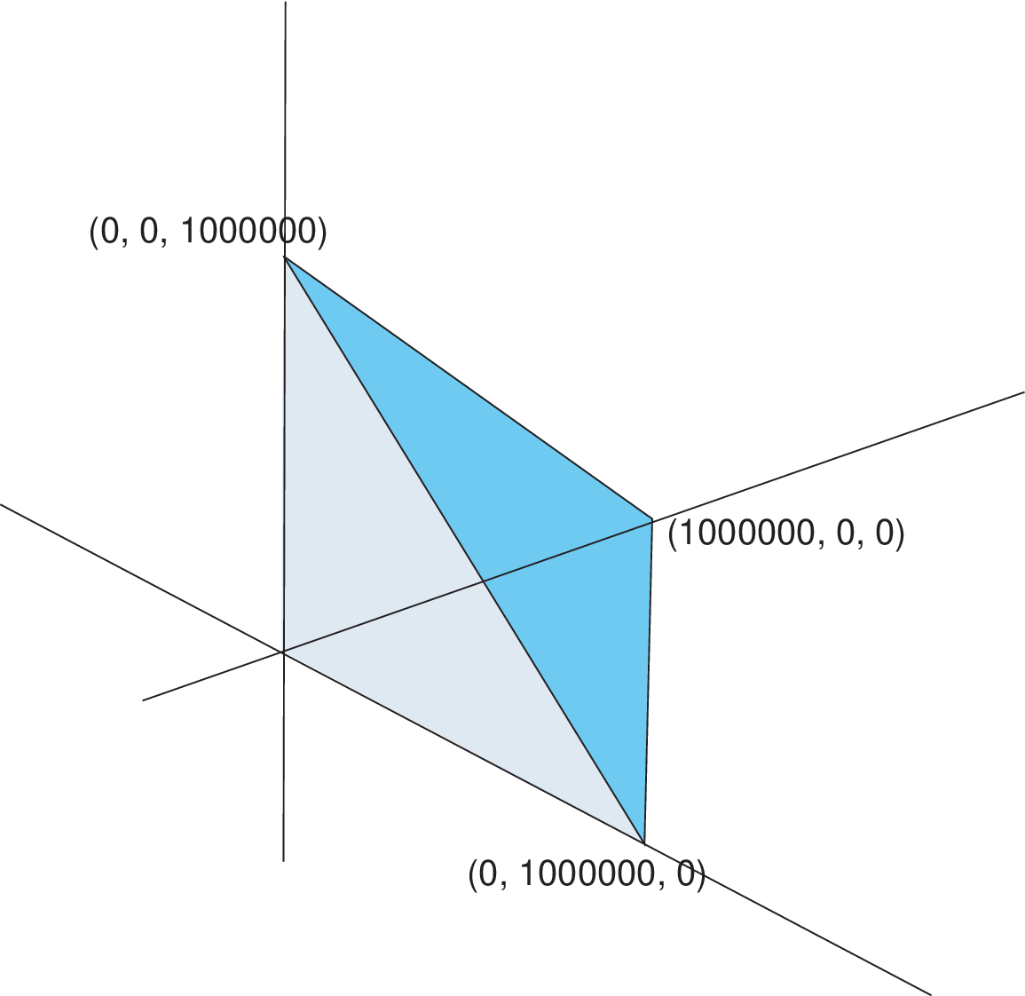
f(P,z)\hskip 11.74988pt=\hskip 11.74988pt\frac{1}{(1-z_{1})(1-z_{2})(1-z_{3})}+\frac{z_{1}^{1000000}}{(1-z_{1}^{-1}z_{2})(1-z_{1}^{-1}z_{3})(1-z_{1}^{-1})}

+\frac{z_{2}^{1000000}}{(1-z_{1}z_{2}^{-1})(1-z_{2}^{-1}z_{3})(1-z_{2}^{-1})}+\frac{z_{3}^{1000000}}{(1-z_{1}z_{3}^{-1})(1-z_{2}z_{3}^{-1})(1-z_{3}^{-1})}.

One might ask how one can compute Barvinok’s rational functions for the input polyhedron. The following theorem tells us that there is an algorithm created by Barvinok 1994 to compute Barvinok’s rational functions from the input polyhedron in polynomial time in fixed dimension. We will describe a variation of the algorithm in Chapter 4.

Theorem 1.1.

(Barvinok 1994, Theorem 5.4) Fix the dimension $d$ . Then there exists a polynomial time algorithm which for a given rational polyhedron $P\subset\mathbb{R}^{d}$ , computes $f(P,z)$ in the form of (1.2) in polynomial time.

We do not want to expand Barvinok’s rational functions because expanding them causes exponential complexity. So, if we want to perform operations on sets via generating functions, such as taking unions, intersections, projections, and complements, we want to do it directly with Barvinok’s rational functions without expanding them. The Hadamard product of Laurent power series is a very useful tool for Boolean operations on sets via Barvinok’s rational functions.

Definition 1.2.

Let $g_{1}$ and $g_{2}$ be Laurent power series in $z\in{\mathbb{C}}^{d}$ such that $g_{1}(z)=\sum_{m\in{\mathbb{Z}}^{d}}a_{m}z^{m}$ and $g_{2}(z)=\sum_{m\in{\mathbb{Z}}^{d}}b_{m}z^{m}$ . Then the Hadamard product $g=g_{1}*g_{2}$ is the power series such that:

g(z)=\sum_{m\in{\mathbb{Z}}^{d}}a_{m}b_{m}z^{m}.

Hadamard products of Laurent power series are one of the most important tools to prove theorems in this thesis. They are used for taking unions of sets, intersections of sets, and set difference via short rational functions without expanding them. We will show how to compute the Hadamard product of Laurent power series $g_{1}$ and $g_{2}$ given in the form of rational functions. Let $p_{1},p_{2},a_{11},\dots,a_{1k}\in{\mathbb{Z}}^{d}$ and $a_{21},\dots,a_{2k}\in{\mathbb{Z}}^{d}$ . Suppose we are given the Laurent power series $g_{1}$ and $g_{2}$ in the form:

g_{1}=\frac{z^{p_{1}}}{(1-z^{a_{11}})\dots(1-z^{a_{1k}})}\mbox{ and }g_{2}=\frac{z^{p_{2}}}{(1-z^{a_{21}})\dots(1-z^{a_{2k}})}.

(1.3)

Here is an outline of the algorithm to take the Hadamard product of two Laurent power series via Barvinok’s rational functions.

Algorithm 1.3.

(Barvinok and Woods 2003, Lemma 3.4)

Input: Laurent power series $g_{1}$ and $g_{2}$ in the form of (1.3).

Output: The Hadamard product $g_{1}*g_{2}$ of $g_{1}$ and $g_{2}$ in the form of a rational function.

Step 1: If $a_{1j}>0$ or $a_{2j}>0$ , then apply the identity:

\frac{z^{p}_{j}}{1-z^{a}_{j}}=-\frac{z^{p-a}_{j}}{1-z^{-a}_{j}},

to reverse the direction of $a_{1j}$ or $a_{2j}$ .

Step 2: Let $P\subset\mathbb{R}^{2k}=\{(\xi_{1},\xi_{2},\dots,\xi_{2k}):\xi_{i}\in\mathbb{R}\mbox{ for }i=1,2,\dots,2k\}$ be a rational polyhedron defined by the equation:

p_{1}+\xi_{1}a_{11}+\dots+\xi_{k}a_{1k}=p_{2}+\xi_{k+1}a_{21}+\dots+\xi_{2k}a_{2k},

and inequalities

\xi_{i}\geq 0\mbox{ for }i=1,2,\dots,2k.

Step 3: Using Theorem 1.1, we compute:

f(P,x)=\sum_{i\in I}\pm\frac{x^{u_{i}}}{(1-x^{v_{1,i}})(1-x^{v_{2,i}})\dots(1-x^{v_{2k,i}})},

for $u_{i},v_{i,j}\in{\mathbb{Z}}^{2k}$ .

Step 5: Apply the monomial substitution $\Phi:{\mathbb{C}}^{2k}\to{\mathbb{C}}^{k}$ such that:

x_{1}=z^{a_{11}},\dots,x_{k}=z^{a_{1k}},x_{k+1}=1,\dots,x_{2k}=1

to the function $f(P,x)$ .

Step 4: Return $g_{1}*g_{2}=z^{p_{1}}\Phi(f(P,x))$ .

1.2 Computer Algebra and applications to Statistics

One focus of this thesis is applying Barvinok’s rational functions to Statistics and Mixed Integer Programming. First we consider the connection between Computational Algebra and contingency tables in Statistics.

Definition 1.4.

A $s$ -table of size $(n_{1},\dots,n_{s})$ is an array of non-negative integers $v=(v_{i_{1},\dots,i_{s}})$ , $1\leq i_{j}\leq n_{j}$ . For $0\leq L<s$ , an $L$ -marginal of $v$ is any of the $s\choose L$ possible $L$ -tables obtained by summing the entries over all but $L$ indices.

Example 1.5.

Consider a $3$ -table $X=(x_{ijk})$ of size $(m\mbox{, }n\mbox{, }p)$ , where $m$ , $n$ , and $p$ are natural numbers. Let the integral matrices $M_{1}=(a_{jk})$ , $M_{2}=(b_{ik})$ , and $M_{3}=(c_{ij})$ be $2$ -marginals of $X$ , where $M_{1}$ , $M_{2}$ , and $M_{3}$ are integral matrices of type $n\times p$ , $m\times p$ , and $m\times n$ respectively. Then, a $3$ -table $X=(x_{ijk})$ of size $(m\mbox{, }n\mbox{, }p)$ with given marginals satisfies the system of equations and inequalities:

\begin{array}[]{ll}\sum_{i=1}^{m}x_{ijk}=a_{jk}\mbox{, }(j=1,2,...,n\mbox{, }k=1,2,...,p),\\ \sum_{j=1}^{n}x_{ijk}=b_{ik}\mbox{, }(i=1,2,...,m\mbox{, }k=1,2,...,p),\\ \sum_{k=1}^{p}x_{ijk}=c_{ij}\mbox{, }(i=1,2,...,m\mbox{, }j=1,2,...,n),\\ x_{ijk}\geq 0\mbox{, }(i=1,2,...,m\mbox{, }j=1,2,...,n\mbox{, }k=1,2,...,p).\\ \end{array}

(1.4)

Such tables appear naturally in Statistics and Operations Research under various names such as multi-way contingency tables, or tabular data. We consider the table counting problem and table sampling problem:

Problem 1.6.

(Table counting problem)

Given a prescribed collection of marginals, how many $d$ -tables are there that share these marginals?

Problem 1.7.

(Table sampling problem)

Given a prescribed collection of marginals, generate typical tables that share these marginals.

The table counting problem and table sampling problem have several applications in statistical analysis, in particular for independence testing, and have been the focus of much research (Anderson and Fienberg 2001; De Loera and Onn 2002; Diaconis and Sturmfels 1998; Dobra and Sullivant 2002; Rapallo 2003). Given a specified collection of marginals for $d$ -tables of size $(n_{1},\dots,n_{d})$ (possibly together with specified lower and upper bounds on some of the table entries) the associated multi-index transportation polytope is the set of all non-negative real valued arrays satisfying the given marginals and entry bounds specified in the system of equations and inequalities, such as formulas (1.4) for a $3$ -table given in Example 1.5. The counting problem is the same as counting the number of integer points in the associated multi-index transportation polytope.

In this thesis, one of the main tools to solve the table counting problems and table sampling problems is Computational Algebra. We consider a special ideal in the multivariate polynomial ring, namely a toric ideal $I_{A}$ associate to the given integral matrix $A$ . We compute the Gröbner basis associate to the toric ideal $I_{A}$ . Then we apply Gröbner bases of the toric ideal $I_{A}$ to the table counting problem and the table sampling problem. Here, we would like to remind the reader of some definitions. Cox et al. 1997 and Sturmfels 1996 are very good references for details. Let us denote ${\mathbb{Z}}^{d}_{+}:=\{x\in{\mathbb{Z}}^{d}:x\geq 0\}$ and ${\mathbb{Z}}_{+}:=\{x\in{\mathbb{Z}}:x\geq 0\}$ .

Definition 1.8.

Let $K$ be any field and let $K[x]=K[x_{1},x_{2},\dots,x_{d}]$ be the polynomial ring in $d$ indeterminates. A monomial is a product of powers of variables in $K[x]$ , i.e. $x^{\alpha_{1}}_{1}x_{2}^{\alpha_{2}}\dots x^{\alpha_{d}}_{d}$ , where $\alpha_{1},\,\alpha_{2},\,\dots,\,\alpha_{d}\in{\mathbb{Z}}_{+}$ .

Definition 1.9.

Let $K$ be any field and let $K[x]=K[x_{1},x_{2},\dots,x_{d}]$ be the polynomial ring in $d$ indeterminates. Let $I\subset K[x]$ . Then we call $I$ an ideal if it satisfies the following:

•

$f+g\in I$ for all $f,\,g\in I$ .
•

$af\in I$ for all $f\in I$ and all $a\in K[x]$ .

Note that by Hilbert basis theorem (Cox et al. 1997, Chapter 2, section 5, Theorem 4) every ideal in $K[x]$ is generated by finitely many elements in $K[x]$ .

Definition 1.10.

Let $\prec$ be a total order on ${\mathbb{Z}}_{+}^{d}$ . We call $\prec$ a term order if it satisfies the following:

•

For any $\alpha,\,\beta,\,\delta\in{\mathbb{Z}}_{+}^{d}$ , $\alpha\prec\beta\rightarrow\alpha+\delta\prec\beta+\delta$ .
•

For any $\alpha\in{\mathbb{Z}}^{d}_{+}\backslash\{0\}$ , $0\prec\alpha$ .

A term order on ${\mathbb{Z}}^{d}_{+}$ gives a term order on the monomials of $K[x]$ by setting a bijection map from ${\mathbb{Z}}^{d}_{+}$ to $S\subset K[x]$ , where $S$ is the set of all monomials in $K[x]$ , such that $(a_{1},\,a_{2},\,\dots,\,a_{d})\to x_{1}^{a_{1}}x_{2}^{a_{2}}\dots x_{d}^{a_{d}}$ .

Definition 1.11.

(The lexicographic term ordering) Let $\alpha,\,\,\beta\in{\mathbb{Z}}^{d}_{+}$ . We say $\alpha\prec_{lex}\beta$ if the left most non-zero entry of $\alpha-\beta\in{\mathbb{Z}}^{d}$ is negative. We write $x^{\alpha}\prec_{lex}x^{\beta}$ if $\alpha\prec_{lex}\beta$ .

For example, if we have $(3,2,7)$ and $(3,5,2)$ in $\mathbb{R}^{3}$ , then we have $(3,2,7)-(3,5,2)=(0,-3,5)$ . So, $(3,2,7)\prec_{lex}(3,5,2)$ and $x_{1}^{3}x_{2}^{2}x_{3}^{7}\prec_{lex}x_{1}^{3}x_{2}^{5}x_{3}^{2}$ . One notices that the lexicographic term ordering is a term order.

We can also define a term order from a vector $c$ , as we described in Definition 1.10, by the following method: we make this vector $c$ into a term order $\prec_{c}$ such that for all $\alpha,\,\beta\in{\mathbb{Z}}^{d}_{+}$ , $\alpha\prec_{c}\beta$ if

•

$c\cdot\alpha<c\cdot\beta$ or
•

$c\alpha=c\beta$ and $\alpha\prec_{lex}\beta$ .

For example, suppose $c=(1,0,2)$ and if we have $(3,2,7)$ and $(3,5,2)$ in $\mathbb{R}^{3}$ , then we have $(1,0,2)\cdot(3,2,7)=17$ and $(1,0,2)\cdot(3,5,2)=13$ . So, since $(1,0,2)\cdot(3,5,2)<(1,0,2)\cdot(3,2,7)$ , we have $(3,5,2)\prec_{c}(3,2,7)$ and $x_{1}^{3}x_{2}^{5}x_{3}^{2}\prec_{c}x_{1}^{3}x_{2}^{2}x_{3}^{7}$ .

In general, any term order is defined by a $d\times d$ integral matrix $W$ . We represent a term order $\prec$ on monomials in $x_{1},\ldots,x_{d}$ by an integral $d\times d$ -matrix $W$ as in (Mora and Robbiano 1998). Two monomials satisfy $\,x^{\alpha}\prec x^{\beta}\,$ if and only if $W\alpha$ is lexicographically smaller than $W\beta$ . In other words, if $w_{1},\ldots,w_{d}$ denote the rows of $W$ , there is some $j\in\{1,\ldots,d\}$ such that $w_{i}\alpha=w_{i}\beta$ for $i<j$ , and $w_{j}\alpha<w_{j}\beta$ . For example, $W=I_{d}$ describes the lexicographic term ordering. We will denote by $\prec_{W}$ the term order defined by $W$ .

Definition 1.12.

Let $K$ be any field and let $K[x]=K[x_{1},x_{2},\dots,x_{d}]$ be the polynomial ring in $d$ indeterminates. Given a term order $\prec$ , every non-zero polynomial $f\in K[x]$ has a unique initial monomial, denoted $in_{\prec}(f)$ . If $I$ is an ideal in $K[x]$ , then its initial ideal is the monomial ideal

in_{\prec}(I):=<in_{\prec}(f):f\in I>.

The monomials which do not lie in $in_{\prec}(I)$ are called standard monomials. A finite subset $G\subset I$ is called a Gröbner basis for $I$ with respect to $\prec$ if $in_{\prec}(I)$ is generated by $\{in_{\prec}(g):g\in G\}.$ A Gröbner basis is called reduced if for any two distinct elements $g,\bar{g}\in G$ , no terms of $\bar{g}$ is divisible by $in_{\prec}(g)$ .

Proposition 1.13.

(Cox et al. 1997, Proposition 1, Chapter 6)

Let $G:=\{g_{1},g_{2},\dots,g_{k}\}$ be a Gröbner basis for an ideal $I\subset K[x]$ and let $f\in K[x]$ . Then there exists a unique $r\in K[x]$ such that:

•

No term of $r$ is divisible by any of leading term of $g_{i}$ , for all $i=1,2,\dots,k$ .
•

There is $g\in I$ such that $f=g+r$ .

In particular $r$ is the remainder on division of $f$ by $G$ , and $r$ is unique no matter how the elements of $G$ are listed when using the division algorithm.

The remainder $r$ for $f\in K[x]$ is called the normal form of $f$ . Note that the reduced Gröbner basis is unique. This thesis concentrates in a special kind of ideals $I$ in $K[x]=K[x_{1},x_{2},\dots,x_{d}]$ , which are called toric ideals. Toric ideals find applications in Integer Programming, Computational Algebra, and Computational Statistics (Sturmfels 1996).

Definition 1.14.

Fix a subset $A=\{a_{1},a_{2},\dots,a_{d}\}$ of ${\mathbb{Z}}^{n}$ .
Each vector $a_{i}$ is identified with a monomial in the Laurent polynomial ring $K[\pm t]:=K[t,t^{2},\dots,t^{d},t^{-1},t^{-2},\dots,t^{-d}]$ . Consider the homomorphism induced by the monomial map

\hat{\pi}:K[x]\to K[\pm t],\,x_{i}\to t^{a_{i}}.

Then the kernel of the homomorphism $\hat{\pi}$ is called the toric ideal of $A$ .

The following lemma describes the set of generators of a toric ideal $I_{A}$ associated to the integral matrix $A$ .

Lemma 1.15.

(Sturmfels 1996, Lemma 4.1) The toric ideal $I_{A}$ is spanned as a $K$ -vector space by the set of binomials

\{x^{u}-x^{v}\,:\,\,u,\,v\in{\mathbb{Z}}^{d}_{+},\,\,Au=Av\}.

The main theorem on Chapter 2 concerns a new way to compute the toric ideal $I_{A}$ of the integral matrix $A$ .

Now we are ready to discuss applications of Computational Algebra to Computational Statistics. As we mentioned earlier, a toric ideal $I_{A}$ and the Gröbner basis associated to $I_{A}$ find applications to Computational Statistics (Sturmfels 1996). Here we would like to discuss how we can apply Gröbner bases to solve the table counting and table sampling problems. First of all, we will remind the reader of the definition of Markov bases associate to the given integral matrix $A$ (Diaconis and Sturmfels 1998).

Definition 1.16.

Let $P=\{x\in\mathbb{R}^{d}:Ax=b,x\geq 0\}\not=\emptyset$ , where $A\in\mathbb{Z}^{n\times d}$ and $b\in{\mathbb{Z}}^{n}$ , and let $M$ be a finite set such that $M\subset\{x\in{\mathbb{Z}}^{d}:Ax=0\}$ . Then we define the graph $G_{b}$ such that:

•

Nodes of $G_{b}$ are lattice points inside $P$ .
•

Draw a undirected edge between a node $u$ and a node $v$ if and only if $u-v\in M$ .

Then we call $M$ a Markov basis of the toric ideal associate to a matrix $A$ if $G_{b}$ is connected for all $b$ with $P\not=\emptyset$ . If $M$ is minimal with respect to inclusion, then we call $M$ a minimal Markov basis.

Note that, in general, a minimal Markov basis is not necessarily unique. A Markov basis can be used for randomly sampling data and random walks on contingency tables (Diaconis and Gangolli 1995; Diaconis and Sturmfels 1998). We will describe the Monte Carlo Markov Chain algorithm which uses Markov bases to create random walks on contingency tables. We can also define a Gröbner basis using a graph $G_{b}$ .

Lemma 1.17.

(Sturmfels 1996, Theorem 5.5) Let $P=\{x\in\mathbb{R}^{d}:Ax=b,x\geq 0\}\not=\emptyset$ , where $A\in\mathbb{Z}^{n\times d}$ and $b\in{\mathbb{Z}}^{n}$ . Let $M$ be a finite set such that $M\subset\{x\in{\mathbb{Z}}^{d}:Ax=0\}$ and let $\prec$ be any term order on ${\mathbb{N}}^{d}$ . Then we define the graph $G_{b}$ such that:

•

Nodes of $G_{b}$ are lattice points inside $P$ .
•

Draw a directed edge between a node $u$ and a node $v$ if and only if $u\prec v$ for $u-v\in M$ .

If $G_{b}$ is acyclic and has a unique sink for all $b$ with $P\not=\emptyset$ , then $M$ is a Gröbner basis for a toric ideal associate to a matrix $A$ with respect to $\prec$ .

Notice that if $M$ is a Gröbner basis then this implies $M$ is a Markov basis because if we have an acyclic directed graph with a unique sink, then it has to be connected. However, note that not all Markov bases are Gröbner bases.

Remark: Gröbner bases provide a way to generate Markov bases for a wide variety of problems where no natural set of moves were known.

Example 1.18.

Suppose we have $2\times 3$ tables with given marginals.

				Total
	? ? ?	? ? ?	? ? ?	6
	? ? ?	? ? ?	? ? ?	6
Total	4	4	4

Table 1.1:

2\times 3

tables with

1

-marginals.

There are $19$ tables with these marginals for $2\times 3$ tables in Table 1.1.

Up to signs, there are $3$ elements in the Markov basis.

Figure 1.4 gives a connected graph for a Markov basis for $2\times 3$ tables. An element of the Markov basis is a undirected edge between integral points in the polytope.

From here on, we focus on Markov bases for contingency tables. Why do we care about Markov bases for contingency tables? We care about them because using Markov bases, we can estimate the number of tables by Monte Carlo Markov Chain (MCMC) algorithm (Diaconis and Sturmfels 1998). Diaconis and Saloff-Coste 1995 also showed that the rate of convergence for MCMC is $\delta^{2}$ , where $\delta$ is the diameter of the graph $G_{b}$ . The outline of MCMC algorithm is the following:

Algorithm 1.19.

(Diaconis and Sturmfels 1998, Lemma 2.1)

(Random walk on a graph)

Input: A Markov basis $M$ of a graph $G_{b}$ defined by the set of contingency tables with given marginals and an initial node $f_{0}$ in $G_{b}$ .

Output: A sample from the hypergeometric distribution $\sigma(\cdot)$ on $G_{b}$ .

1.

Set $f:=f_{0}$ and set $t=0$ .
2.

While ( $t<\delta^{2}$ )
- •
  
  Choose $u\in M$ uniformly and a sign $\epsilon=\pm 1$ with probability $1/2$ each independently from $u$ .
- •
  
  If $f+\epsilon u\geq 0$ then move the chain from $f$ to $f+\epsilon u$ with probability $\min\{\sigma(f+\epsilon u)/\sigma(f),1\}$ . If not, stay at $f$ . Set $t=t+1$ .

Diaconis and Sturmfels 1998 showed that this random walk on the graph $G_{b}$ is a connected, reversible, aperiodic Markov chain on $G_{b}$ which converges to the hypergeometric distribution (Diaconis and Sturmfels 1998, Lemma 2.1). With the random walk on the graph $G_{b}$ , we apply it to approximating the number of lattice points in a convex rational polytope $P$ . The idea for approximating the number of lattice points in a convex polytope $P$ is the following:

Suppose we take a sequence of draws $H:=\{n_{1},n_{2}\dots,n_{m}\}$ randomly from the uniform distribution over $P$ . Let $p(n_{i})=1/|P|$ be the uniform distribution over $P$ . If we can simulate a lattice point $n_{i}\in P$ from a distribution $q(\cdot)$ , where $q(t)>0$ for all $t\in P$ , then we have

E[\frac{1}{q(t)}]=\sum_{t\in P}\frac{1}{q(t)}q(t)=|P|.

Hence by the Strong Law of Large Number (Durrett 2000, (7.1) on page 56), the estimation of $|P|$ is:

\frac{1}{m}\sum_{i=1}^{m}\frac{1}{q(n_{i})}.

1.3 Algorithms for counting

Enumerating the lattice points in a given polytope and counting the number of lattice points in a given polytope is very useful to Computational Statistics (De Loera and Onn 2002; Diaconis and Gangolli 1995; Diaconis and Sturmfels 1998; Dobra and Sullivant 2002; Rapallo 2003). So, in the next section, we will briefly discuss methods to count exactly the number of lattice points in a given convex polyhedron. Barvinok’s method will be fully discussed in Chapter 4

Using the multivariate generating function $f(P,z)$ for a polytope $P$ , we can count the number of lattice points inside $P$ . In fact, the number of lattice points inside $P$ is $f(P,(1,1,\dots,1))$ .

Example: Let $P$ be the quadrangle with vertices $V_{1}=(0,0)$ , $V_{2}=(5,0)$ , $V_{3}=(4,2)$ , and $V_{4}=(0,2)$ .

Then we have:

If we substitute $z_{1}=1$ and $z_{2}=1$ in $f(P,z)$ , then we have $f(P,(1,1))=16$ , which is also the number of lattice points inside $P$ .

We can use Barvinok’s rational functions to count the number of lattice points inside a polytope. Notice that, unfortunately, the point $(z_{1},z_{2},\dots,z_{d})=(1,1,\dots,1)$ is a pole of Barvinok’s rational functions. Thus, we cannot directly substitute $(z_{1},z_{2},\dots,z_{d})=(1,1,\dots,1)$ into $f(P,z)$ . Instead, we compute $\lim_{z\to(1,\dots,1)}f(P,z)$ , which is the number of lattice points inside $P$ . In this thesis, we apply the residue calculus to compute $\lim_{z\to(1,\dots,1)}f(P,z)$ . We will discuss how to compute this limit via the residue calculus in Section 4.1.2.

Several “analytic” algorithms have been proposed by many authors Baldoni-Silva and Vergne 2002; Beck 2003; Lasserre and Zeron 2002; Lasserre and Zeron 2003; MacMahon 1960; Pemantle and Wilson 2003. A couple of these methods have been implemented and appear as the fastest for unimodular polyhedra. However, only Barvinok’s method has been implemented for arbitrary rational polytopes. Consider, for example, Beck’s method: let $M_{i}$ be the columns of the matrix $M$ . We can interpret $P(M,b)\cap\mathbb{Z}^{d}$ as the Taylor coefficient of $z^{b}$ for the function $\Pi_{j=1}^{d}\frac{1}{(1-z^{M_{j}})}$ . One approach to obtain the particular coefficient is to use the residue theorem. For example, it was seen in Beck 2000 that

P(M,b)\cap\mathbb{Z}^{d}=\frac{1}{(2\pi i)^{m}}\int_{\left|z_{1}\right|=\epsilon_{1}}\cdots\int_{\left|z_{m}\right|=\epsilon_{m}}\frac{z_{1}^{-b_{1}-1}\cdots z_{m}^{-b_{m}-1}}{\left(1-z^{M_{1}}\right)\cdots\left(1-z^{M_{d}}\right)}\ dz\ .

Here $0<\epsilon_{1},\dots,\epsilon_{m}<1$ are different numbers such that we can expand all the $\displaystyle\frac{1}{1-z^{M_{k}}}$ into the power series about $0$ . It is possible to do a partial fraction decomposition of the integrand into a sum of simple fractions. This was done very successfully to carry out very hard computations regarding the Birkhoff polytopes (Beck 2003). Vergne and collaborators have recently developed a powerful general theory about the multivariate rational functions $\Pi_{j=1}^{d}\frac{1}{(1-z^{M_{j}})}$ (Baldoni-Silva and Vergne 2002; Szenes and Vergne 2002). Experimental results show that it is a very fast method for unimodular polytopes (Baldoni-Silva et al. 2003). Pemantle and Wilson (Pemantle and Wilson 2003) have pursued an even more general computational theory of rational generating functions where the denominators are not necessarily products of linear forms.

Recently, Lasserre and Zeron 2003 introduced another method to enumerate the lattice points in a rational convex polyhedron. Suppose we have a rational convex polyhedron $P_{y}=\{x\in\mathbb{R}^{d}:Ax=y,\,\,x\geq 0\}$ , where $A=(A_{ij})\in{\mathbb{Z}}^{n\times d}$ and $b\in{\mathbb{Z}}^{n}$ . Then we define the function

f(z):=\sum_{x\in P_{y}\cap{\mathbb{Z}}^{d}}e^{c\cdot x},

(1.5)

where $c\in{\mathbb{Z}}^{d}$ is small enough so that $f(z)$ is well defined. A tool which Lasserre and Zeron 2003 use is a generating function $F:{\mathbb{C}}^{n}\to{\mathbb{C}}$ :

z\to F(z):=\sum_{y\in{\mathbb{Z}}^{n}}f(y)z^{y}.

(1.6)

Note that the generating functions in (1.5) and (1.6) are different from Barvinok’s.

Let us define $P^{*}_{0}:=\{b\in\mathbb{R}^{d}:b\cdot x\geq 0,\,x\in P_{0}\}$ and $\Gamma:=\{c\in\mathbb{R}^{d}:-c>b,\,\mbox{ for some }b\in P^{*}_{0}\}$ . Suppose $A_{i}$ is the $i$ th column of a matrix $A$ . Then we have the following lemma.

Lemma 1.20.

(Lasserre and Zeron 2003, Proposition 2.4)

Let $f$ and $F$ be functions defined in (1.5) and (1.6), and let $c\in\Gamma$ . Then:

F(z)=\prod_{k=1}^{d}\frac{1}{(1-e^{c}z_{1}^{A_{1k}}\dots z_{n}^{A_{nk}})},

on the domain $(|z_{1}|,\dots,|z_{n}|)\in\{y\in\mathbb{R}^{n}:y>0,\,e^{c_{k}}x^{A_{k}}<1,k=1,\dots,d\}$ .

Definition 1.21.

(Lasserre and Zeron 2003, Definition 2.1) Let $p\in{\mathbb{N}}$ satisfy $n\leq p\leq d$ and let $\nu=\{\nu_{1},\dots,\nu_{p}\}\subset{\mathbb{N}}$ be an ordered set with cardinality $|\nu|=p$ and $1\leq\nu_{1}\leq\dots\leq\nu_{p}\leq d$ . Then

1.

$\nu$ is said to be a basis of order $p$ if the $n\times p$ submatrix $A_{\nu}=[A_{\nu_{1}}|\dots|A_{\nu_{p}}]$ has the maximum rank.
2.

For $n\leq p\leq d$ , let $J_{p}:=\{\nu\subset\{1,\dots,d\}|\nu\mbox{ is a basis of order }p\}$ .

Then Lasserre and Zeron 2003 show how to invert the generating function $F(z)$ in order to obtain the exact value of $f(y)$ . First, they determine an appropriate expansion of the generating function in the form:

F(z)=\sum_{\sigma\in J_{n}}\frac{Q_{\sigma}}{\prod_{k\in\sigma}(1-e^{c_{k}}z^{A_{k}})},

(1.7)

where the coefficient $Q_{\sigma}:{\mathbb{C}}^{n}\to{\mathbb{C}}$ are rational functions with a finite Laurent series

z\to Q_{\sigma}=\sum_{\beta\in{\mathbb{Z}}^{n},||\beta||\leq M}Q_{\sigma,\beta}z^{\beta},

(1.8)

for a strictly positive integer $M$ . Then they apply the following theorem to obtain $f(y)$ .

Theorem 1.22.

(Lasserre and Zeron 2003, Theorem 2.6)

Let $A\in{\mathbb{Z}}^{n\times d}$ be of maximal rank, let $f$ be as in (1.5) with $c\in\Gamma$ . Assume that the generating function $F$ in (1.6) satisfies (1.7) and (1.8). Then,

f(y)=\sum_{\sigma\in J_{n}}\sum_{\beta\in{\mathbb{Z}}^{n},||\beta||\leq M}Q_{\sigma,\beta}E_{\sigma}(y-\beta)

with

E_{\sigma}(y-\beta)=\left\{\begin{array}[]{ll}e^{c\cdot_{\sigma}x},\mbox{ if }x:=A^{-1}_{\sigma}(y-\beta)\in{\mathbb{N}}^{n},\\ 0\mbox{ otherwise;}\\ \end{array}\right.

where $c_{\sigma}=(c_{\sigma_{1}},\dots,c_{\sigma_{n}})$ .

The main point is that as soon as we have $f(y)$ with sufficiently small $c$ vector, if we send $c_{i}\to 0$ for $i=1,2,\dots d$ , then we can obtain the number of lattice points inside a convex rational polytope $P_{y}$ (if $P_{y}$ is a unbounded polyhedron, then this limit does not converge).

1.4 Applications to Mixed Integer Programming

Now we explain the connections between Barvinok’s rational functions and integer programming problems. We consider an integer linear programming problem:

Question 1.23.

(Integer Programming)

Suppose $A\in Z^{n\times d}$ , $c\in Z^{d}$ , and $b\in Z^{n}$ . We assume that the rank of $A$ is $n$ . Given a polyhedron $P=\{x\in\mathbb{R}^{d}:Ax=b,\,x\geq 0\}$ , we want to solve the following problem:

\mbox{(IP) maximize}\ c\cdot x\ \mbox{subject to}\hskip 11.74988ptx\in P,\ \,x\in{\mathbb{Z}}^{d}.

These problems are called integer programming problems and we know that this problem is NP-hard (Karp 1972). However, Lenstra 1983 showed that if we fixed the dimension, we can solve (IP) in polynomial time. Originally, Barvinok’s counting algorithm relied on H. Lenstra’s polynomial time algorithm for Integer Programming in a fixed number of variables (Lenstra 1983), but shortly after Barvinok’s breakthrough, Dyer and Kannan 1993 showed that this step can be replaced by a short-vector computation using the $LLL$ algorithm. Therefore, using binary search, one can turn Barvinok’s counting oracle into an algorithm that solves integer programming problems with a fixed number of variables in polynomial time (i.e. by counting the number of lattice points in $P$ that satisfy $c\cdot x\geq\alpha$ , we can narrow the range for the maximum value of $c\cdot x$ , then we iteratively look for the largest $\alpha$ where the count is non-zero). This idea was proposed by Barvinok in (Barvinok and Pommersheim 1999). We call this IP algorithm the BBS algorithm.

To solve more general problems one might want to consider some variables as real numbers, instead of all integers. Thus one can set the following problems:

Question 1.24.

(Mixed Integer Programming)

\mbox{(MIP) maximize}\ c\cdot x\ \mbox{subject to}\hskip 11.74988ptx\in P,\ \,x_{i}\in{\mathbb{Z}}\ \mbox{if the index}\ i\in\ J\subset[d].

One notices that linear programming problems form a subset of (MIP) problems, i.e. $J=\emptyset$ and also integer programming problems form a subset of (MIP) problems, i.e. $J=[d]$ .

As we mentioned earlier, we can define the term order from a cost vector $c$ , as we described in Definition 1.10. From this term order $\prec_{c}$ , as soon as we have the reduced Gröbner basis with the term order $\prec_{c}$ , we can solve the integer programming problem $\min\{c\cdot x:x\in P\cap{\mathbb{Z}}^{d}\}$ . A sketch of an algorithm is the following:

Algorithm 1.25.

(Sturmfels 1996, Algorithm 5.6)

Input: A cost vector $c\in{\mathbb{Z}}^{d}$ , a matrix $A\in{\mathbb{Z}}^{n\times d}$ , a vector $b\in{\mathbb{Z}}^{n}$ and a feasible solution $v_{0}\in P\cap{\mathbb{Z}}^{d}$ , where $P:=\{x\in\mathbb{R}^{d}:Ax=b,\,\,x\geq 0\}$ .

Output: An optimal solution and the optimal value of minimize $c\cdot x$ subject to $x\in P\cap{\mathbb{Z}}^{d}$ .

Step 1: Compute the Gröbner basis with the term order $\prec_{c}$ .

Step 2: Compute the normal form $x^{u}$ of $x^{v_{0}}$ and return $u$ and $cu$ , which are an optimal solution and the optimal value, respectively.

One notices that Algorithm 1.25 outputs the optimal value and an optimal solution for minimization. Trivially if one wants to have the optimal value and an optimal solution for maximization such as (IP), one can set $c=-c$ and apply Algorithm 1.25.

Definition 1.26.

Suppose we have a rational convex polyhedron $P\subset\mathbb{R}^{d}$ and suppose we have an integer programming problem such that maximize $c\cdot x$ subject to $x\in P\cap{\mathbb{Z}}^{d}$ . Also suppose a feasible solution $x_{0}\in P\cap{\mathbb{Z}}^{d}$ is given. Then we call an integral vector $t\in{\mathbb{Z}}^{d}$ an augmenting vector if $c(x_{0}+t)>cx_{0}$ . A finite set which contains all augmenting vectors is called a test set.

There has been considerable activity in the area of test sets and augmentation methods (e.g. Graver, integral basis method, etc. See Aardal et al. 2002c; Thomas 2001). One notices from Algorithm 1.25 that the Gröbner basis of a toric ideal $I_{A}$ associated to the integral matrix $A$ with respect to a term order $\prec_{c}$ is a test set for an integer programming problem $\min\{c\cdot x:Ax=b,\,\,x\geq 0,,x\in{\mathbb{Z}}^{d}\}$ .

In 2003, Lasserre observed a new method for solving integer programming problems using Barvinok’s short rational functions, which is different from the BBS algorithm. We consider the integer programming problem $maximize\{c\cdot x:Ax\leq b,x\geq 0,x\in{\mathbb{Z}}^{d}\}$ , where $c\in{\mathbb{Z}}^{d}$ , $A\in{\mathbb{Z}}^{m\times d}$ , and $b\in{\mathbb{Z}}^{m}$ . This problem is equivalent to Problem 1.23, because using Hermite normal form, we can project the polytope $P$ down into a lower dimension until the dimension of $P$ equals to the dimension of ambience space. We assume that the input system of inequalities $Ax\leq b,x\geq 0$ defines a bounded polytope $P\subset\mathbb{R}^{d}$ , such that $P\cap{\mathbb{Z}}^{d}$ is nonempty. As before, all integer points are encoded as a short rational function $f(P,z)$ in Equation (1.2) for $P$ , where the rational function is given in Barvinok’s form. Remember that if we were to expand Equation (1.2) into monomials (generally a very bad idea!) we would get $f(P,z)=\sum_{\alpha\in P\cap{\mathbb{Z}}^{d}}z^{\alpha}$ . For a given $c\in{\mathbb{Z}}^{d}$ , we make the substitution $z_{i}=t^{c_{i}}$ , Equation (1.2) yields a univariate rational function in $t$ :

f(P,t)=\sum_{i\in I}{\pm\frac{t^{c\cdot u_{i}}}{\prod_{j=1}^{d}(1-t^{c\cdot v_{ij}})}}.

(1.9)

The key observation is that if we make that substitution directly into the monomial expansion of $f(P,z)$ , we have $z^{\alpha}\to t^{c\cdot\alpha}$ . Moreover we would obtain the relation

f(P,t)=\sum_{\alpha\in P\cap{\mathbb{Z}}^{d}}t^{c\cdot\alpha}=kt^{M}+\mbox{(lower degree terms)},

(1.10)

where $M$ is the optimal value of our Integer Program and where $k$ counts the number of optimal integer solutions. Unfortunately, in practice, $M$ and the number of lattice points in $P$ may be huge and we need to avoid the monomial expansion step altogether. All computations have to be done by manipulating short rational functions in (1.9).

Lasserre 2004 suggested the following approach: for $i\in I$ , define sets $\eta_{i}$ by $\eta_{i}=\{j\in\{1,...,d\}:c\cdot v_{ij}>0\}$ , and define vectors $w_{i}$ by $w_{i}=u_{i}-\sum_{j\in\eta_{i}}v_{ij}.$ Let $n_{i}$ denote the cardinality of $\eta_{i}$ . Now we define $M=\max\{c\cdot w_{i}:i\in I\}$ , $S=\{i\in I:c\cdot w_{i}=M\}$ and we set $\sigma=\sum_{i\in S}E_{i}(-1)^{n_{i}}$ . Note that $M$ simply denotes the highest exponent of $t$ appearing in the expansions of the rational functions defined for each $i\in I$ in (1.9). The number $\sigma$ is in fact the sum of the coefficients of $t^{M}$ in these expressions, that is, $\sigma$ is the coefficient of $t^{M}$ in $f(P,t)$ . Now with these definitions and notation we can state the following result proved by Lasserre 2004.

Theorem 1.27.

(Lasserre 2004, Theorem 3.1)

If $c\cdot v_{ij}\neq 0$ for all $i\in I,j\in\{1,\ldots,d\}$ , and if $\sigma\neq 0$ , then M is the optimal value $\pi$ of Integer Program $maximize\{c\cdot x:Ax\leq b,x\geq 0,x\in{\mathbb{Z}}^{d}\}$ .

1.5 Summary of results in this thesis

In this section, we would like to summarize all of the results in this thesis. In Chapter 2, the first theorem concerns the computation of the toric ideal $I_{A}$ of the matrix $A$ .

Theorem 1.28.

Let $A\in\mathbb{Z}^{n\times d}$ and a term order $\prec_{W}$ specified by a matrix $W$ . Assuming that $n$ and $d$ are fixed, then there are algorithms, that run in polynomial time in the size of the input data, to perform the following four tasks:

1.

Compute a short rational function $G$ which represents the reduced Gröbner basis of the toric ideal $I_{A}$ with respect to the term order $\prec_{W}$ .
2.

Decide whether the input monomial $x^{a}$ is in normal form with respect to $G$ .
3.

Perform one step of the division algorithm modulo $G$ .
4.

Compute the normal form of the input monomial $x^{a}$ modulo the Gröbner basis $G$ .

The proof of Theorem 1.28 will be given in Section 2.1. Special attention will be paid to the Projection Theorem (Barvinok and Woods 2003, Theorem 1.7) since the projection of short rational functions is the most difficult step to implement. Its practical efficiency has yet to be investigated.

Theorem 1.28 can be applied to prove many interesting theorems and corollaries in Computational Statistics and Integer Programming. The following corollary can be proved by Theorem 1.28 and the fact that a Gröbner basis associated to a toric ideal $I_{A}$ of the integral matrix $A$ is a Markov basis associate to $A$ .

Corollary 1.29.

Let $A\in{\mathbb{Z}}^{n\times d}$ , where $d$ and $n$ are fixed. There is a polynomial time algorithm to compute a multivariate rational generating function for a Markov basis $M$ associated to $A$ . This is presented as a short sum of rational functions.

From Algorithm 1.25, one can see that Theorem 1.28 proves the following theorem:

Corollary 1.30.

Let $A\in{\mathbb{Z}}^{n\times d}$ , $b\in{\mathbb{Z}}^{n}$ , and $c\in{\mathbb{Z}}^{d}$ . Given a polyhedron $P=\{x\in\mathbb{R}^{d}:Ax=b,\,x\geq 0\}$ , compute the mixed integer programming problem, via the Gröbner basis associated a toric ideal $I_{A}$ with the term order $\prec_{c}$ obtained by Barvinok’s rational functions in Theorem 1.28,

\mbox{maximize}\ c\cdot x\ \mbox{subject to}\hskip 11.74988ptx\in P,\ \,x\in{\mathbb{Z}}^{d},

in polynomial time if we fix $n$ and $d$ .

Chapter 2 introduces a new algorithm, improving on Barvinok’s original work, which we call the homogenized Barvinok algorithm. Like the original version in (Barvinok 1994), it runs in polynomial time when the dimension is fixed. Then we will apply the homogenized Barvinok’s algorithm to Commutative Algebra. The Hilbert series of $S$ is the rational generating function $\,\sum_{a\in S}x^{a}$ . Barvinok and Woods (2003) showed that this Hilbert series can be computed as a short rational generating function in polynomial time for fixed dimension. We show that this computation can be done without the Projection Theorem (Lemma 2.4) when the semigroup is known to be normal.

Theorem 1.31.

Under the hypothesis that the ambient dimension $d$ is fixed,

1.

the Ehrhart series of a rational convex polytope given by linear inequalities can be computed in polynomial time. The Projection Theorem is not used in the algorithm.
2.

The same applies to computing the Hilbert series of a normal semigroup $S$ .

Chapter 3 discusses Integer and Mixed Integer Programming. We describe a new mixed integer programming algorithm via Barvinok’s rational functions. This is a different approach from the method via the reduced Gröbner basis of the toric ideal $I_{A}$ associated to the integral matrix $A$ . It is based on Theorem 1.27 in Chapter 1. Also in Chapter 3 we give a new algorithm to compute the optimal value and an optimal solution for any Integer Linear Program via Barvinok’s rational functions. In Section 3.2, we will show the performance of the BBS algorithm in some knapsack problems. Chapter 3 will show a proof of the following theorem:

Theorem 1.32.

Let $A\in{\mathbb{Z}}^{m\times d}$ , $b\in{\mathbb{Z}}^{m}$ , $c\in{\mathbb{Z}}^{d}$ , and assume that number of variables $d$ is fixed. Suppose $P:=\{x\in\mathbb{R}^{d}:Ax\leq b,x\geq 0\}$ is a rational convex polytope in $\mathbb{R}^{d}$ . Given the mixed-integer programming problem

\mbox{maximize}\ c\cdot x\ \mbox{subject to}\hskip 11.74988ptx\in\{x\in\mathbb{R}^{d}:x\in P,\ x_{i}\in{\mathbb{Z}}\ \mbox{for}\ \ i\in J\subset\{1,\ldots,d\}\},

(A) We can use rational functions to encode the set of vectors (the $(A,b,c)$ -test set):

$\{u-v:u\ \hbox{is a}\ c-\hbox{optimal solution},\ v\ \hbox{feasible solution},u,v\in{\mathbb{Z}}^{d}\},$

and then solve the MIP problem in time polynomial in the size of the input.

(B) More strongly, the $(A,b,c)$ test set can be replaced by smaller test sets, such as Graver bases or reduced Gröbner bases.

We improve Lasserre’s heuristic and give a third deterministic IP algorithm based on Barvinok’s rational function algorithms, the digging algorithm. In this case the algorithm can have an exponential number of steps even for fixed dimension, but performs well in practice. See Section 3.2 for details.

Chapter 4 concentrates on computational experiments and explains details of the implementation of the software package LattE. We implemented the BBS algorithm and the digging algorithm in the second release of the computer software LattE. We solved several challenging knapsack problems and compared the performance of LattE with the mixed-integer programming solver CPLEX version 6.6. In fact the digging algorithm is often surpassed by what we call the single cone digging algorithm. See Section 4.5 for computational tests. In Section 4.2 we present some computational experience with our current implementation of LattE. We report on experiments with families of well-known rational polytopes: multiway contingency tables, knapsack type problems, and rational polygons. We demonstrate that LattE competes with commercial branch-and-bound software and solves very hard instances and enumerates some examples that had never been done before. We also tested the performance in the case of two-way contingency tables and Kostant’s partition function where special purpose software has been written already Baldoni-Silva and Vergne 2002; Beck 2003; De Loera and Sturmfels 2001; Mount 2000. In Section 4.3 we present formulas for the Ehrhart quasi-polynomials of several hypersimplices and truncations of cubes (e.g. the 24 cell). We show solid evidence that Barvinok’s ideas are practical and can be used to solve non-trivial problems, both in Integer Programming and Symbolic Computing.

In Section 4.4 we present some experimental results with the homogenized Barvinok algorithm. It was recently implemented in LattE. Like we will show in Chapter 2, it runs in polynomial time when the dimension is fixed. But it performs much better in practice (1) when computing the Ehrhart series of polytopes with few facets but many vertices; (2) when computing the Hilbert series of normal semigroup rings. We show its effectiveness by solving the classical counting problems for $5\times 5$ magic squares (all row, column and diagonal sums are equal) and $3\times 3\times 3\times 3$ magic cubes (all line sums in the 4 possible coordinate directions and the sums along main diagonal entries are equal). Our computational results are presented in Theorem 4.11.

Chapter 2 Gröbner bases of toric ideals via short rational functions

The main techniques used in this thesis came from the Algebra of polynomial ideals. We use special sets of generators called Gröbner bases. We deal with ideals associated with polyhedra that are called toric ideals (see definitions 1.1). In this chapter we present polynomial-time algorithms for computing with toric ideals and semigroup rings in fixed dimension. For background on these algebraic objects and their interplay with polyhedral geometry see (Stanley 1996; Sturmfels 1996; Villarreal 2001). Our results are a direct application of recent results by Barvinok and Woods (2003) on short encodings of rational generating functions (such as Hilbert series).

2.1 Computing Toric Ideals

From now on and without loss of generality we will assume that $ker(A)\cap\mathbb{R}_{\geq 0}^{d}=\{0\}$ . This condition is not restrictive because toric ideal problems can be reduced to this particular case via homogenization of the problem. Our assumption implies that for all $b$ , the convex polyhedron $\,P\,=\,\{\,u\in\mathbb{R}^{d}\,\,:\,\,A\cdot u=b\,\,\hbox{and}\,\,u\geq 0\,\}\,$ is a polytope (i.e. a bounded polytope) or the empty set. We begin by recalling some useful results of Barvinok and Woods (2003):

Lemma 2.1.

(Barvinok and Woods 2003, Theorem 3.6) Let $S_{1},S_{2}$ be finite subsets of ${\mathbb{Z}}^{d}$ , for $d$ fixed. Let $f(S_{1},x)$ and $f(S_{2},x)$ be their generating functions, given as short rational functions with at most $k$ binomials in each denominator. Then there exists a polynomial time algorithm, which, given $f(S_{i},x)$ , computes

f(S_{1}\cap S_{2},x)\hskip 11.74988pt=\hskip 11.74988pt\sum_{i\in I}\gamma_{i}\cdot\frac{x^{u_{i}}}{(1-x^{v_{i1}})\dots(1-x^{v_{is}})}

with $s\leq 2k$ , where the $\gamma_{i}$ are rational numbers, $u_{i},v_{ij}$ are nonzero integer vectors, and $I$ is a polynomial-size index set.

The following lemma was proved by Barvinok and Woods using Lemma 2.1:

Lemma 2.2.

(Barvinok and Woods 2003, Corollary 3.7) Let $S_{1},S_{2},\dots,S_{m}$ be finite subsets of ${\mathbb{Z}}^{d}$ , for $d$ fixed. Let $f(S_{i},x)$ for $i=1\dots m$ be their generating functions, given as short rational functions with at most $k$ binomials in each denominator. Then there exists a polynomial time algorithm, in the input size, which computes

f(S_{1}\cup S_{2}\cup\dots S_{m},x)\hskip 11.74988pt=\hskip 11.74988pt\sum_{i\in I}\gamma_{i}\cdot\frac{x^{u_{i}}}{(1-x^{v_{i1}})\dots(1-x^{v_{is}})}

with $s\leq 2k$ , where the $\gamma_{i}$ are rational numbers, $u_{i},v_{ij}$ are nonzero integer vectors, and $I$ is a polynomial-size index set. Similarly one can compute in polynomial time $f(S_{1}\backslash S_{2},x)$ as a short rational function.

We will use the Intersection Lemma and the Boolean Operation Lemma to extract special monomials present in the expansion of a generating function. The essential step in the intersection algorithm is the use of the Hadamard product (see Algorithm 1.3) and a special monomial substitution. The Hadamard product is a bilinear operation on rational functions (we denote it by $*$ ). The computation is carried out for pairs of summands as in (1.2). Note that the Hadamard product $m_{1}*m_{2}$ of two monomials $m_{1},m_{2}$ is zero unless $m_{1}=m_{2}$ . We present an example of computing intersections.

Example 2.3.

Let $S_{i}=\{\,x\in\mathbb{R}:i-2\leq x\leq i\,\}\cap{\mathbb{Z}}$ for $i=1,2$ . We rewrite their rational generating functions as in the proof of Theorem 3.6 in (Barvinok and Woods 2003): $f(S_{1},z)=\frac{z^{-1}}{(1-z)}+\frac{z}{(1-z^{-1})}=\frac{-z^{-2}}{(1-z^{-1})}+\frac{z}{(1-z^{-1})}=g_{11}+g_{12},$ and $f(S_{2},z)=\frac{1}{(1-z)}+\frac{z^{2}}{(1-z^{-1})}=\frac{-z^{-1}}{(1-z^{-1})}+\frac{z^{2}}{(1-z^{-1})}=g_{21}+g_{22}$ .

We need to compute four Hadamard products between rational functions $g_{ij}$ ,whose denominators are products of binomials and whose numerators are monomials. Lemma 3.4 in Barvinok and Woods 2003 says that, these Hadamard products are essentially the same as computing the rational function, as in Equation (1.2), of the auxiliary polyhedron $\{(\epsilon_{1},\epsilon_{2})|p_{1}+a_{1}\epsilon_{1}=p_{2}+a_{2}\epsilon_{2},\,\epsilon_{i}\geq 0\}$ . Here $p_{1},p_{2}$ are the exponents of numerators of ${g_{ij}}\ ^{\prime}s$ involved and $a_{1},a_{2}$ are the exponents of the binomial denominators. For example, the Hadamard product $g_{11}*g_{22}$ corresponds to the polyhedron $\,\{(\epsilon_{1},\epsilon_{2})|\epsilon_{2}=4+\epsilon_{1},\,\epsilon_{i}\geq 0\}$ . The contribution of this half line is $-\frac{z^{-2}}{(1-z^{-1})}$ . We find

	$\displaystyle f(S_{1},z)*f(S_{2},z)\hskip 11.74988pt=$	$\displaystyle g_{11}g_{21}+g_{12}g_{22}+g_{12}g_{21}+g_{11}g_{22}$
	$\displaystyle=$	$\displaystyle\hskip 11.74988pt\frac{z^{-2}}{(1-z^{-1})}+\frac{z}{(1-z^{-1})}-\frac{z^{-1}}{(1-z^{-1})}-\frac{z^{-2}}{(1-z^{-1})}$
	$\displaystyle=$	$\displaystyle\frac{z-z^{-1}}{1-z^{-1}}\hskip 11.74988pt=\hskip 11.74988pt1+z\hskip 11.74988pt=\hskip 11.74988ptf(S_{1}\cap S_{2},z).$

Another key subroutine introduced by Barvinok and Woods is the following Projection Theorem. In Lemmas 2.1, 2.2, and 2.4, the dimension $d$ is assumed to be fixed.

Lemma 2.4.

(Barvinok and Woods 2003, Theorem 1.7) Assume the dimension $d$ is a fixed constant. Consider a rational polytope $P\subset\mathbb{R}^{d}$ and a linear map $T:{\mathbb{Z}}^{d}\rightarrow{\mathbb{Z}}^{k}$ . There is a polynomial time algorithm which computes a short representation of the generating function $\,f\bigl(T(P\cap{\mathbb{Z}}^{d}),x\bigr)$ .

Defining a term order $\prec_{W}$ by a $d\times d$ integral matrix $W$ (see details in Section 1.2), we have the following lemma.

Lemma 2.5.

Let $S\subset{\mathbb{Z}}^{d}_{+}$ be a finite set of lattice points in the positive orthant. Suppose the polynomial $\,f(S,x)=\sum_{\beta\in S}x^{\beta}\,$ is represented as a short rational function and let $\prec_{W}$ be a term order. We can extract the (unique) leading monomial of $f(S,x)$ with respect to $\prec_{W}$ in polynomial time.

Proof: The term order $\prec_{W}$ is represented by an integer matrix $W$ . For each of the rows $w_{j}$ of $W$ we perform a monomial substitution $x_{i}:=x^{\prime}_{i}t^{w_{ji}}$ . Note that $t$ is a “dummy variable” that we will use to keep track of elimination. Such a monomial substitution can be computed in polynomial time by (Barvinok and Woods 2003, Theorem 2.6). The effect is that the polynomial $f(S,x)$ gets replaced by a polynomial in the $t$ and the $x^{\prime}s$ . After each substitution we determine the degree in $t$ . This is done as follows: We want to do calculations in univariate polynomials since this is faster so we consider the polynomial $g(t)=f(S,1,t)$ , where all variables except $t$ are set to the constant one. Clearly the degree of $g(t)$ in $t$ is the same as the degree of $f(S,x^{\prime},t)$ . We create the interval polynomial $i_{[p,q]}(t)=\sum^{q}_{i=p}t^{i}$ which obviously has a short rational function representation. Compute the Hadamard product of $i_{[p,q]}(t)$ with $g(t)$ . This yields those monomials whose degree in the variable $t$ lies between $p$ and $q$ . We will keep shrinking the interval $[p,q]$ until we find the degree. We need a bound for the degree in $t$ of $g(t)$ to start a binary search. An upper bound $U$ can be found via linear programming or via the estimate in Theorem 3.1 of (Lasserre 2004) which is an easy manipulation of the numerator and denominator of the fractions in $g(t)$ . It is clear that $\log(U)$ is polynomially bounded. In no more than $\log(U)$ steps one can determine the degree in $t$ of $f(S,x,t)$ by using a standard binary search algorithm.

Let $\alpha$ be a polynomial-size upper bound on the highest total degree of a monomial appearing in the generating function $f(S,x)$ . We can again apply linear programming or the estimate of (Lasserre 2004) to compute such an $\alpha$ (just as we computed $U$ before). Once the highest degree $r$ in $t$ is known, we compute the Hadamard product of $f(S,x,t)$ and $t^{r}h(x)$ , where $h(x)$ is the rational generating function encoding the lattice points contained inside the box $[0,\alpha]^{d}$ . This will capture only the desired monomials. Then compute the limit as $t$ approaches $1$ . This can be done in polynomial time using residue techniques. The limit represents the subseries $\,H(S,x)=\sum_{\beta\cdot w_{j}=r}x^{\beta}$ . Repeat the monomial and highest degree search for the row $w_{j+1}$ , $w_{j+2}$ , etc. Since $\prec_{W}$ is a term order, after doing this $d$ times we will have only one single monomial left, the desired leading monomial.

One has to be careful when using earlier Lemmas (especially the projection theorem) that the sets in question are finite. We need the following well-known bound:

Lemma 2.6.

(Sturmfels 1996, Lemma 4.6 and Theorem 4.7) Let $M$ be equal to $(n+1)(d-n)D(A)$ , where $A$ is an $n\times d$ integral matrix and $D(A)$ is the biggest $n\times n$ subdeterminant of $A$ in absolute value. Any entry of an exponent vector of any reduced Gröbner basis for the toric ideal $I_{A}$ is less than $M$ .

Proposition 2.7.

Let $A\in\mathbb{Z}^{n\times d}$ , $W\in{\mathbb{Z}}^{d\times d}$ specifying a term order $\prec_{W}$ . Assume that $n$ and $d$ are fixed.

1) There is a polynomial time algorithm to compute a short rational function $G$ which represents a universal Gröbner basis of $I_{A}$ .

2) Suppose we are given the term order $\prec_{W}$ and a short rational function encoding a finite set of binomials $x^{u}-x^{v}$ now expressed as the sum of monomials $\sum x^{u}y^{v}$ . Assume $M$ is an integer positive bound on the degree of any variable for any of the monomials. One can compute in polynomial time a short rational function encoding only those binomials $x^{u}-x^{v}$ that satisfy $x^{v}\prec_{W}x^{u}$ .

3) Suppose we are given a sum of short rational functions $f(x)$ which is identical, in its monomial expansion, to a single monomial $x^{a}$ . Then in polynomial time we can recover the (unique) exponent vector $a$ .

Proof: 1) Set $\,M=(n+1)(d-n)D(A)\,$ where $D(A)$ is again the largest absolute value of any $n\times n$ -subdeterminant of $A$ . Using Barvinok’s algorithm in (Barvinok 1994), we compute the following generating function in $2d$ variables:

G(x,y)\hskip 11.74988pt=\hskip 11.74988pt\sum\bigl\{\,x^{u}y^{v}\,\,:\,\,Au=Av\,\,\,\hbox{and}\,\,0\leq u_{i},v_{i}\leq M\,\bigr\}.

This is the sum over all lattice points in a rational polytope. Lemma 2.6 above implies that the toric ideal $I_{A}$ is generated by the finite set of binomials $x^{u}-x^{v}$ corresponding to the terms $x^{u}y^{v}$ in $G(x,y)$ . Moreover, these binomials are a universal Gröbner basis of $I_{A}$ .

2) Denote by $w_{i}$ the $i$ -th row of the matrix $W$ which specifies the term order. Suppose we are given a short rational generating function $\,G_{0}(x,y)\,=\,\sum x^{u}y^{v}\,$ representing a set of binomials $\,x^{u}-x^{v}$ in $I_{A}$ , for instance $G_{0}=G$ in part (1). In the following steps, we will alter the series so that a term $x^{u}y^{v}$ gets removed whenever $u$ is not bigger than $v$ in the term order $\prec_{W}$ . Starting with $H_{0}=G_{0}$ , we perform Hadamard products with short rational functions $f(S;x,y)$ for $S\subset{\mathbb{Z}}^{2d}$ .

Set $H_{i}=H_{i-1}*f(\{(u,v):w_{i}u=w_{i}v,\ 0\leq u_{j},v_{j}\leq M,\ j=1\dots d\})$ , and $G_{i}=H_{i-1}*f(\{(u,v):w_{i}u\geq w_{i}v+1,\ 0\leq u_{j},v_{j}\leq M\ j=1\dots d\}).$ All monomials $x^{u}y^{v}\in G_{j}$ have the property that $w_{i}u=w_{i}v$ for $i<j$ , $w_{j}u>w_{j}v$ , and thus $v\prec_{W}u$ . On the other hand, if $v\prec_{W}u$ then there is some $j$ such that $w_{i}u=w_{i}v$ for $i<j$ , $w_{j}u>w_{j}v$ , and we can conclude that $x^{u}y^{v}\in G_{j}$ . Note that $H=G_{1}\cup G_{2}\cup\ldots\cup G_{d}$ is actually a disjoint union of sets. The rational function that gives the union, can be computed in polynomial time by Lemma 2.2. In practice, the rational generating functions representing the $G_{i}$ ’s can be simply added together. The short rational function $H$ encodes exactly those binomials in $G_{0}$ that are correctly ordered with respect to $\prec_{W}$ . We have proved our claim since all of the above constructions can be done in polynomial time.

3) Given $f(x)$ we can compute in polynomial time the partial derivative $\partial f(x)/\partial x_{i}$ . This puts the exponent of $x_{i}$ as a coefficient of the unique monomial. Computing the derivative can be done in polynomial time by the quotient and product derivative rules. Each time we differentiate a short rational function of the form

\frac{x^{b_{i}}}{(1-x^{c_{1,i}})(1-x^{c_{2,i}})\dots(1-x^{c_{d,i}})}

we add polynomially many (binomial type) factors to the numerator. The factors in the numerators should be expanded into monomials to have again summands in short rational canonical form $\frac{x^{b_{i}}}{(1-x^{c_{1,i}})(1-x^{c_{2,i}})\dots(1-x^{c_{d,i}})}$ . Note that at most $2^{d}$ monomials appear each time ( $d$ is a constant). Finally, if we take the limit when all variables $x_{i}$ go to one we will get the desired exponent.

Example 2.8.

Using LattE we compute the set of all binomials of degree less than or equal $10000$ in the toric ideal $I_{A}$ of the matrix $\,A\,=\,\left[\begin{array}[]{cccc}1&1&1&1\\ \vskip 3.0pt plus 1.0pt minus 1.0pt\cr 0&1&2&3\end{array}\right]$ . This matrix represents the Twisted Cubic Curve in algebraic geometry. We find that there are exactly $195281738790588958143425$ such binomials. Each binomial is encoded as a monomial $\,x_{1}^{u_{1}}x_{2}^{u_{2}}x_{3}^{u_{3}}x_{4}^{u_{4}}y_{1}^{v_{1}}y_{2}^{v_{2}}y_{3}^{v_{3}}y_{4}^{v_{4}}$ . The computation takes about $40$ seconds. The output is a sum of $538$ simple rational functions of the form a monomial divided by a product such as $\left(1-{\frac{x_{{3}}y_{{4}}}{x_{{1}}y_{{2}}}}\right)\left(1-{\frac{x_{{1}}x_{{4}}y_{{2}}}{x_{{3}}}}\right)\left(1-x_{{1}}y_{{1}}\right)\left(1-x_{{1}}x_{{3}}{y_{{2}}}^{2}\right)\left(1-x_{{3}}y_{{3}}\right)\left(1-x_{{2}}y_{{2}}\right)$ .

Proof of Theorem 1.28

The proof of Theorem 1.28 will require us to project and intersect sets of lattice points represented by rational functions. We cannot, in principle, do those operations for infinite sets of lattice points. Fortunately, in our setting it is possible to restrict our attention to finite sets. Besides Lemma 2.6 for the size of exponents of Gröbner bases, we need a bound for the exponents of normal form monomials:

Lemma 2.9.

Let $x^{u}$ be the normal form of $x^{a}$ with respect to the reduced Gröbner basis $G$ of a toric ideal $I_{A}$ for the term order $\prec_{W}$ (associated to the matrix $W$ ). Every coordinate of $u$ is bounded above by $L=(n+1)dD(A){\tilde{a}}$ , where $D(A)$ is the biggest subdeterminant of $A$ in absolute value, $\tilde{a}$ denotes the largest coordinate of the exponent vector $a$ .

Proof: We note that $u$ is a point in the (bounded) convex polytope defined by the following inequalities in $v$ : $Av=Aa$ , and $v\geq 0$ (it is forced to be bounded for all $a$ because we assumed $ker(A)\cap\mathbb{R}_{\geq 0}^{d}=\{0\}$ ). Thus each coordinate of $u$ is bounded above by the corresponding coordinate of some vertex of this polytope. Let $v$ be such a vertex. The non-zero entries of $v$ are given by $B^{-1}Aa$ where $B$ is a maximal non-singular square submatrix of $A$ . Clearly, each entry of $B^{-1}A$ is bounded above by $D(A)$ , and hence each entry of $v$ is bounded above by $L$ . We conclude that $L$ is an upper bound for the coordinates of $u$ .

Proof of Theorem 1.28: Proposition 2.7 gives a Gröbner basis for the toric ideal $I_{A}$ in polynomial time. We now show how to get the reduced Gröbner basis from it in three easy polynomial time steps. The input is the the $n\times d$ integral matrix $A$ and the $d\times d$ term order matrix $W$ . The algorithm for claim (1) of Theorem 1.28 has three steps:

Step 1. Let $M$ be equal to $(n+1)(d-n)D(A)$ , as in Lemma 2.6, for given input matrix $A$ . As in Proposition 2.7, compute the generating function which encodes binomials of highest degree $M$ on variables that generate $I_{A}$ :

f(x,y)\hskip 11.74988pt=\hskip 11.74988pt\sum\bigl\{\,x^{u}y^{v}\,\,:\,\,Au=Av\,\,\hbox{and}\,\,0\leq u_{j},v_{j}\leq M\,\,\hbox{for}\,\,j=1\dots d\bigr\},

Next we wish to remove from $f(x,y)$ all incorrectly ordered binomials (i.e. those monomials $x^{u}y^{v}$ with $u\prec_{W}v$ instead of the other way around). We do this using part 2 of Proposition 2.7. We obtain from it a collection $G_{0},G_{1},\dots,G_{d}$ of rational functions encoding disjoint sets of lattice points. We call $\bar{f}(x,y)$ the generating function representing the union of $G_{0},\dots,G_{d}$ . This can be computed in polynomial time by adding the rational functions of the $G_{i}$ together (since they are disjoint). The reader should notice that this updated $\bar{f}(x,y)$ contains only those monomials of the old $f(x,y)$ that are now correctly ordered.

Let $g_{i}(x)$ be the projection of $G_{i}$ onto the first group of $x$ -variables and denote by $g(x)$ the rational function that represents the union of the $g_{i}(x)$ . The rational function $g(x)$ can be computed in polynomial time by the projection theorem of Barvinok-Woods, i.e. Lemma 2.4. It is important to note that $g(x)$ is the result of projecting $\bar{f}(x,y)$ into the first group of variables. This is true because a linear projection of the union of disjoint lattice point sets (i.e. those represented by $G_{i}$ ) equals the union of the projections of the individual sets. In conclusion, $g(x)$ is the sum over all non-standard monomials having degree at most $M$ in any variable.

Step 2. Write $r(x,M)=\prod\limits_{i=1}^{d}(\frac{1}{1-x_{i}}+\frac{x_{i}^{M}}{1-x_{i}^{-1}})$ for the generating function of all $x$ -monomials having degree at most $M$ in any variable. Note that this is a large, but finite, set of monomials. We compute the following Hadamard product of $d$ rational functions in $x$ and Boolean complements (we denote them by $\backslash$ ):

\biggl(r(x,M)\backslash x_{1}\cdot g(x)\biggr)*\biggl(r(x,M)\backslash x_{2}\cdot g(x)\biggr)*\cdots*\biggl(r(x,M)\backslash x_{d}\cdot g(x)\biggr).

This is the generating function over those monomials all of whose proper factors are standard modulo the toric ideal $I_{A}$ and whose degree in any variable is at most $M$ .

Step 3. Let $h(x,y)$ denote the ordinary product of the resulting rational function from Step 2 with

r(y,M)\backslash g(y)=\sum\bigl\{\,y^{v}\,\,:\,\,v\,\,\hbox{standard monomial modulo}\,I_{A}\,\hbox{of highest degree $M$}\bigr\}.

Thus $h(x,y)$ is the sum of all monomials $x^{u}y^{v}$ such that $x^{v}$ is standard and $x^{u}$ is a monomial all of whose proper factors are standard monomials modulo the toric ideal $I_{A}$ and, finally, the highest degree in any variable is at most $M$ .

Compute the Hadamard product $G(x,y):=\,\bar{f}(x,y)*h(x,y)$ . This is a short rational representation of a polynomial, namely, it is the sum over all monomials $x^{u}y^{v}$ such that the binomial $x^{u}-x^{v}$ is in the reduced Gröbner basis of $I_{A}$ with respect to $W$ and $x^{v}\prec_{W}x^{u}$ . This completes the proof of the first claim of Theorem 1.28.

We next give the algorithm that solves claims 2 and 3 of Theorem 1.28. This will be done in four steps (1,2,3,4). We are given an input monomial $x^{a}$ for which we aim to determine whether it is already in normal form.

Step 4 Perform Steps 1,2,3. Let $G(x,y)$ be the reduced Gröbner basis of $I_{A}$ with respect to the term order $W$ encoded by the rational function obtained at the end of Step 3. Let $r(x,{\tilde{a}})$ be, as before, the rational function of all monomials having degree less than ${\tilde{a}}$ on any variable. Thus $G^{\prime}(x,y)=r(x,{\tilde{a}})\cdot G(x,y)$ consists of all monomials of the form $x^{s}(x^{u}y^{v})$ where $x^{u}-x^{v}$ is a binomial of the Gröbner basis and where $0\leq s\leq\tilde{a}$ . Thus $x^{s}x^{u}$ is a monomial divisible by some leading term of the Gröbner basis.

Given a monomial $x^{a}$ consider $b(x,y)$ , the rational function representing the lattice points of $\,\{(u,v):u=a,\,0\leq v_{j}\leq L\,\,\hbox{for}\,\,j=1\dots d\}$ . The Hadamard product $\,\bar{G}(x,y)=G^{\prime}(x,y)*b(x,y)$ is computable in polynomial time and corresponds to those binomials in $G(x,y)$ that can reduce $x^{a}$ . If $\bar{G}(x,y)$ is empty then $x^{a}$ is in normal form already, otherwise we use Lemma 2.5 and part 3 of Proposition 2.7 to find an element $x^{u}y^{v}\in\bar{G}(x,y)$ and reduce $x^{a}$ to $x^{a-u+v}$ . We may assume that the coefficient of the encoded monomial is one, because we can compute the coefficient in polynomial time using residue techniques, and divide our rational function through by it.

Finally, we present the algorithm for claim 4 in Theorem 1.28 in four steps (1,2,5,6). A curious byproduct of representing Gröbner bases with short rational functions is that the reduction to normal form need not be done by dividing several times anymore.

Step 5. Redo all the calculations of the Steps 1,2,3 using $L=(n+1)dD(A){\tilde{a}}$ from Lemma 2.9 instead of $M$ . Note that the logarithm of $L$ is still bounded by a polynomial in the size of the input data ( $A,W,a$ ). Let $\bar{f}(x,y)$ and $g(x)$ from Step 1,2 (now recomputed with the new bound $L$ ) and compute the Hadamard product

H(x,y)\hskip 11.74988pt:=\hskip 11.74988pt\bar{f}(x,y)*\biggl(\,r(x,L)\cdot\bigl(r(y,L)\backslash g(y)\bigr)\biggr).

This is the sum over all monomials $x^{u}y^{v}$ where $x^{v}$ is the normal form of $x^{u}$ and highest degree of $x^{u}$ on any variable is $L$ . Since we took a high enough degree, by Lemma 2.9, the monomial $x^{a}y^{p}$ , with $x^{p}$ the normal form of $x^{a}$ , is sure to be present.

Step 6. We use $H(x,y)$ as one would use a traditional Gröbner basis of the ideal $I_{A}$ . The normal form of a monomial $x^{a}$ is computed by forming the Hadamard product $H(x,y)*(x^{a}\cdot r(y,L)).$ Since this is strictly speaking a sum of rational functions equal to a single monomial, applying Part 3 of Proposition 2.7 completes the proof of Theorem 1.28.

2.2 Computing Normal Semigroup Rings

We will show in Chapter 4 that a major practical bottleneck of the original Barvinok algorithm in (Barvinok 1994) is the fact that a polytope may have too many vertices. Since originally one visits each vertex to compute a rational function at each tangent cone, the result can be costly. For example, the well-known polytope of semi-magic cubes in the $4\times 4\times 4$ case has over two million vertices, but only 64 linear inequalities describe the polytope. In such cases we propose a homogenization of Barvinok’s algorithm working with a single cone.

There is a second motivation for looking at the homogenization. Barvinok and Woods (Barvinok and Woods 2003) proved that the Hilbert series of semigroup rings can be computed in polynomial time. We show that for normal semigroup rings this can be done simpler and more directly, without using the Projection Theorem.

Given a rational polytope $P$ in $\mathbb{R}^{d-1}$ , we set $i(P,m)=\#\{z\in{\mathbb{Z}}^{d-1}:z\in mP\}$ . The Ehrhart series of $P$ is the generating function $\,\sum_{m=0}^{\infty}i(P,m)t^{m}$ .

Algorithm 2.10 (Homogenized Barvinok algorithm).

Input: A full-dimensional, rational convex polytope $P$ in $\mathbb{R}^{d-1}$ specified by linear inequalities and linear equations.

Output: The Ehrhart series of $P$ .

1.

Place the polytope $P$ into the hyperplane defined by $x_{d}=1$ in $\mathbb{R}^{d}$ . Let $K$ be the $d$ -dimensional cone over $P$ , that is, $K=cone(\{(p,1):p\in P\})$ .
2.

Compute the polar cone $K^{*}$ . The normal vectors of the facets of $K$ are exactly the extreme rays of $K^{*}$ . If the polytope $P$ has far fewer facets then vertices, then the number of rays of the cone $K^{*}$ is small.
3.

Apply Barvinok’s decomposition of $K^{*}$ into unimodular cones. Polarize back each of these cones. It is known, e.g. Corollary 2.8 in (Barvinok and Pommersheim 1999), that by dualizing back we get a unimodular cone decomposition of $K$ . All these cones have the same dimension as $K$ . Retrieve a signed sum of multivariate rational functions which represents the series $\,\sum_{a\in K\cap{\mathbb{Z}}^{d}}x^{a}$ .
4.

Replace the variables $x_{i}$ by $1$ for $i\leq d-1$ and output the resulting series in $t=x_{d}$ . This can be done using the methods in Chapter 4.

One of the key steps in Barvinok’s algorithm is that any cone can be decomposed as the signed sum of (indicator functions of) unimodular cones. We will talk about this in detail on Section 4.1.1, Chapter 4.

Theorem 2.11 (see (Barvinok 1994)).

Fix the dimension $d$ . Then there exists a polynomial time algorithm which decomposes a rational polyhedral cone $K\subset\mathbb{R}^{d}$ into unimodular cones $K_{i}$ with numbers $\epsilon_{i}\in\{-1,1\}$ such that

f(K)\,\,=\,\,\sum_{i\in I}\epsilon_{i}f(K_{i})\mbox{, }\hskip 11.74988pt|I|<\infty.

Originally, Barvinok had pasted together such formulas, one for each vertex of a polytope, using a result of Brion. Using Algorithm 2.10, we can prove Theorem 1.31.

Proof of Theorem 1.31: We first prove part (1). The algorithm solving the problems is Algorithm 2.10. Steps 1 and 2 are polynomial when the dimension is fixed. Step 3 follows from Theorem 2.11. We require a special monomial substitution, possibly with some poles. This can be done in polynomial time by (Barvinok and Woods 2003).

Part (2): Recall the characterization of the integral closure of the semigroup $S$ as the intersection of a pointed polyhedral cone with the lattice ${\mathbb{Z}}^{d}$ . From this it is clear that Algorithm 2.10 computes the desired Hilbert series, with the only modification that the input cone $K$ is given by the rays of the cone and not the facet inequalities. The rays are the generators of the monomial algebra. But, in fixed dimension, one can transfer from the extreme rays representation of the cone to the facet representation of the cone in polynomial time.

Chapter 3 Theoretical applications of rational functions to Mixed Integer Programming

We now discuss how all these ideas can be used in Discrete Optimization.

3.1 The $(A,b,c)$ test set algorithm

In all our discussions below, the input data are an $m\times d$ integral matrix $A$ and an integral $m$ -vector $b$ . For simplicity we assume it describes a polytope $P=\{x\in\mathbb{R}^{d}|Ax\leq b,x\geq 0\}$ . We assume that there are no redundant inequalities and no hidden equations in the system. This polytope $P=\{x\in\mathbb{R}^{d}|Ax\leq b,x\geq 0\}$ is equivalent to the expression of $\{x\in\mathbb{R}^{\bar{d}}|\bar{A}x=b,x\geq 0\}$ , where $\bar{A}\in{\mathbb{Z}}^{m\times\bar{d}}$ and $\bar{d}=m+d$ . We can transform the expression $\{x\in\mathbb{R}^{\bar{d}}|\bar{A}x=b,x\geq 0\}$ to the expression $\{x\in\mathbb{R}^{d}|Ax\leq b,x\geq 0\}$ by projecting down $P$ to a full dimensional polytope with Hermite normal form and we can also transform the expression $\{x\in\mathbb{R}^{d}|Ax\leq b,x\geq 0\}$ to the expression $\{x\in\mathbb{R}^{\bar{d}}|\bar{A}x=b,x\geq 0\}$ by introducing slack variables.

First we would like to remind a reader of Barvinok’s rational functions (see details on Chapter 1). By Theorem 1.1, with a given $P$ , if we fix $d$ there is a polynomial time algorithm to compute Barvinok’s short rational functions in the form of

f(P,z)=\sum_{i\in I}{E_{i}\frac{z^{u_{i}}}{\prod\limits_{j=1}^{d}(1-z^{v_{ij}})}},

(3.1)

where $I$ is a polynomial sized finite indexing set, and where $E_{i}\in\{1,-1\}$ and $u_{i},v_{ij}\in{\mathbb{Z}}^{d}$ for all $i$ and $j$ . In this section we will show how to apply Barvinok’s short rational functions in (3.1) to Mixed Integer Programming.

Proof of Theorem 1.32: We only show the proof of part (A). The proof of part (B) appears in Chapter 2. We first explain how to solve integer programs (where all variables are demanded to be integral). This part of the proof is essentially the proof of Lemma 3.1 given in Hosten and Sturmfels 2003 for the case $Ax=b,\ x\geq 0$ , instead of $Ax\leq b$ , but we emphasize the fact that $b$ is fixed here. We will see how the techniques can be extended to mixed integer programs later. For a positive integer $R$ , let

r(x,R)=\prod\limits_{i=1}^{n}(\frac{1}{1-x_{i}}+\frac{x_{i}^{R}}{1-x_{i}^{-1}})

be the generating function encoding all $x$ -monomials in the positive orthant, having degree at most $R$ in any variable. Note that this is a large, but finite, set of monomials. Suppose $P=\{x\in\mathbb{R}^{d}:Ax\leq b,\,x\geq 0\}$ is a nonempty polytope. Using Barvinok’s algorithm in Barvinok and Pommersheim 1999, compute the following generating function in $2d$ variables:

f(x,y)=\sum\bigl\{\,x^{u}y^{v}\,\,:\,\,Au\leq b,\,Av\leq b,\,u,\,v\geq 0,\mbox{ }c\cdot u-c\cdot v\geq 1,\mbox{ and }u,v\in{\mathbb{Z}}^{d}\bigr\}.

This is possible because we are clearly dealing with the lattice points of a rational polytope. The monomial expansion of $f(x,y)$ exhibits a clear order on the variables: $x^{u}y^{v}$ where $c\cdot u>c\cdot v$ . Hence $v$ is not an optimal solution. In fact, optimal solutions will never appear as exponents in the $y$ variables.

Now let $g(y)$ be the projection of $f(x,y)$ onto the $y$ -variables variables. Thus $g(y)$ is encoding all non-optimal feasible integral vectors (because the exponent vectors of the $x$ ’s are better feasible solutions, by construction), and it can be computed from $f(x,y)$ in polynomial time by Lemma 2.4. Let $V(P)$ be the vertex set of $P$ and choose an integer $R\geq\max\{v_{i}:v\in V(P),\,1\leq i\leq d\}$ (we can find such an integer $R$ via linear programming). Define $f(x,y)$ and $g(x)$ as above and compute the Hadamard product

H(x,y)\hskip 11.74988pt:=\hskip 11.74988ptf(x,y)*\left[\left(r(x,R)-g(x)\right)r(y,R)\right].

This is the sum over all monomials $x^{u}y^{v}$ where $u,\,v\in P$ and where $u$ is an optimal solution. The reader should note that the vectors $u-v$ form a test set (an enormous one), since they can be used to improve from any feasible non-optimal solution $v$ . This set is what we called the $(A,b,c)$ -test set. It should be noted that one may replace $H(x,y)$ by a similar encoding of other test sets, like the Graver test set or a Gröbner basis (see Chapter 2 for details).

We now use $H(x,y)$ as one would use a traditional test set for finding an optimal solution: Find a feasible solution $a$ inside the polytope $P$ using Lemma 2.5 and Barvinok’s Equation (3.1). Improve or augment to an optimal solution by computing the Hadamard product

H(x,y)*\left(y^{a}r(x,R)\right).

The result is the set of monomials of the form $x^{u}y^{a}$ where $u$ is an optimal solution. One monomial of the set, say the lexicographic largest, can be obtained by applying Lemma 2.5. This concludes the proof of the case when all variables are integral.

Now we look at the mixed integer programming case, where only $x_{i}$ with $i\in J\subset\{1,\ldots,d\}$ are required to be integral. Without loss of generality, we may assume that $J=\{r,\ldots,d\}$ for some $r$ , $1\leq r\leq d$ . Thus, splitting $A$ into $(B|C)$ , we may write the polytope $P$ as $\{(x,x^{\prime}):Bx+Cx^{\prime}\leq b,\ x,x^{\prime}\geq 0\}$ where the variables corresponding to $B$ are not demanded to be integral. Consider a vertex optimal solution $\bar{x}$ to the mixed integer problem. The first key observation is that its fractional part can be written as $\bar{x}_{J}=\hat{B}^{-1}(b-C\bar{x}^{\prime})$ where $b-C\bar{x}^{\prime}$ is an integer vector. Here $\hat{B}^{-1}$ denotes the inverse of a submatrix of $B$ . This follows from the theory of linear programming, when we solve the mixed integer program for fixed $x^{\prime}=\bar{x}^{\prime}$ .

The denominators appearing are then contributed by $\hat{B}^{-1}$ . Then every appearing denominator is a factor of $M$ , the least common multiple of all determinants of a square submatrix of $A$ . It is clear $M$ can be computed in polynomial time in the size of the input. This complexity bound holds, since the number of such square submatrices is bounded by a polynomial in $m$ , the number of rows of $A$ , of degree $d$ , the number of columns of $A$ . Moreover, each of these determinants can be computed in time polynomial in the size of the input, and therefore, $M$ itself can be computed in time polynomial in the size of the input in fixed dimension $d$ . Thanks to this information, we know that if we dilate the original polytope $P$ by $M$ , the optimal solutions of the mixed integer program become, in the dilation $MP$ , optimal integral solutions of the problem

\mbox{maximize}\ c\cdot x\ \mbox{subject to}\hskip 11.74988ptx\in MP,\ x\in{\mathbb{Z}}^{d}

with the additional condition that the coordinates with index in $J$ are multiples of $M$ . Ignoring this condition involving multiples of $M$ for a moment, we see that, as we did before, we can obtain an encoding of all optimal improvements as a generating function $H(x,y)$ .

Let $\bar{r}(x,R)=\left[\prod\limits_{i\not\in J}\left(\frac{1}{1-x_{i}}+\frac{x_{i}^{R}}{1-x_{i}^{-1}}\right)\right]\left[\prod\limits_{i\in J}\left(\frac{1}{1-x_{i}^{M}}+\frac{x_{i}^{RM}}{1-x_{i}^{-M}}\right)\right]$ . To extract those vectors whose coordinates indexed by $J$ are multiples of $M$ , we only need to intersect (Hadamard product again) our generating function $H(x,y)$ with the generating function $\bar{r}(x,R)\bar{r}(y,R)$ . Then only those vectors whose coordinates indexed by $J$ are multiples of $M$ remain. This completes the proof of the theorem.

3.2 The Digging Algorithm

In what follows we present a strengthening of Lasserre’s heuristic and discuss how to use Barvinok’s short rational functions to solve integer programs using digging. Suppose $A\in{\mathbb{Z}}^{m\times d}$ , $b\in{\mathbb{Z}}^{m}$ and finite $\Xi\subset{\mathbb{Z}}^{d}$ are given. We consider the family of integer programming problems of the form $\mbox{maximize}\{c\cdot x:Ax\leq b,x\geq 0,x\in{\mathbb{Z}}^{d}\}$ , where $c\in\Xi$ . We assume that the input system of inequalities $Ax\leq b,x\geq 0$ defines a polytope $P\subset\mathbb{R}^{d}$ , such that $P\cap{\mathbb{Z}}^{d}$ is nonempty.

When the hypotheses of Theorem 1.27 are met, from an easy inspection, we could recover the optimal value of an integer program. If we assume that $c$ is chosen randomly from some large cube in ${\mathbb{Z}}^{d}$ , then the first condition is easy to obtain. Unfortunately, our computational experiments (see Section 4.5) indicate that the condition $\sigma\neq 0$ is satisfied only occasionally. Thus an improvement on the approach that Lasserre proposed is needed to make the heuristic terminate in all instances. Here we explain the details of an algorithm that digs for the coefficient of the next highest appearing exponent of $t$ . For simplicity our explanation assumes the easy-to-achieve condition $c\cdot v_{ij}\neq 0$ , for all $v_{ij}$ .

As before, take Equation (3.1) computed via Barvinok’s algorithm. Now, for the given $c$ , we make the substitutions $z_{k}=y_{k}t^{c_{k}}$ , for $k=1,\ldots,d$ . Then substitution into (3.1) yields a sum of multivariate rational functions in the vector variable $y$ and scalar variable $t$ :

g(P;y,t)=\sum_{i\in I}{E_{i}\frac{y^{u_{i}}t^{c\cdot u_{i}}}{\prod_{j=1}^{d}(1-y^{v_{ij}}t^{c\cdot v_{ij}})}}.

(3.2)

On the other hand, the substitution on the left-side of Equation (3.1) gives the following sum of monomials.

g(P;y,t)=\sum_{\alpha\in P\cap{\mathbb{Z}}^{d}}y^{\alpha}t^{c\cdot\alpha}.

(3.3)

Both equations, (3.3) and (3.2), represent the same function $g(P;y,t)$ . Thus, if we compute a Laurent series of (3.2) that shares a region of convergence with the series in (3.3), then the corresponding coefficients of both series must be equal. In particular, because $P$ is a polytope, the series in (3.3) converges almost everywhere. Thus if we compute a Laurent series of (3.2) that has any nonempty region of convergence, then the corresponding coefficients of both series must be equal. Barvinok’s algorithm provides us with the right hand side of (3.2). We need to obtain the coefficient of highest degree in $t$ from the expanded Equation (refeq:d). We compute a Laurent series for it using the following procedure: Apply the identity

\frac{1}{1-y^{v_{ij}}t^{c\cdot v_{ij}}}=\frac{-y^{-v_{ij}}t^{-c\cdot v_{ij}}}{1-y^{-v_{ij}}t^{-c\cdot v_{ij}}}

(3.4)

to Equation (3.2), so that any $v_{ij}$ such that $c\cdot v_{ij}>0$ can be changed in “sign” to be sure that, for all $v_{ij}$ in (3.2), $c\cdot v_{ij}<0$ is satisfied (we may have to change some of the $E_{i}$ , $u_{i}$ and $v_{ij}$ using our identity, but we abuse notation and still refer to the new signs as $E_{i}$ and the new numerator vectors as $u_{i}$ and the new denominator vectors as $v_{ij}$ ). Then, for each of the rational functions in the sum of Equation (3.2) compute a Laurent series of the form

E_{i}\,y^{u_{i}}t^{c\cdot u_{i}}\prod_{j=1}^{d}(1+y^{v_{ij}}t^{c\cdot v_{ij}}+{(y^{v_{ij}}t^{c\cdot v_{ij}})}^{2}+\ldots).

(3.5)

Multiply out each such product of series and add the resultant series. This yields precisely the Laurent series in (3.3). Thus, we have an algorithm to solve integer programs:

Algorithm: (Digging Algorithm):

Input: $A\in{\mathbb{Z}}^{m\times d},\,b\in{\mathbb{Z}}^{m},\,c\in\Xi$ .

Output: optimal value and optimal solution of $\mbox{maximize}\{c\cdot x:Ax\leq b,x\geq 0,x\in{\mathbb{Z}}^{d}\}$ for all $c\in\Xi$ .

Procedure: for each $c\in\Xi$ , do

1.

Use the identity (3.4) as necessary to enforce that all $v_{ij}$ in (3.2) satisfy $c\cdot v_{ij}<0$ .
2.

Via the expansion formulas (3.5), find (3.3) by calculating the terms’ coefficients. Proceed in decreasing order with respect to the degree of $t$ . This can be done because, for each series appearing in the expansion formulas (3.5), the terms of the series are given in decreasing order with respect to the degree of $t$ .
3.

Continue calculating the terms of the expansion (3.3), in decreasing order with respect to the degree of $t$ , until a degree $n$ of $t$ is found such that for some $\alpha\in{\mathbb{Z}}^{d}$ , the coefficient of $y^{\alpha}t^{n}$ is non-zero in the expansion (3.3).
4.

Return “ $n$ ” as the optimal value of the integer program and return $\alpha$ as an optimal solution.

We close this section by noticing that one nice feature of the digging algorithm is if one needs to solve a family of integer programs where only the cost vector $c$ is changing, then Equation (3.2) can be computed once and then apply the steps of the algorithm above for each cost vector to obtain all the optimal values.

Given the polytope $P:=\{x\in\mathbb{R}^{d}:Ax\leq b,\,x\geq 0\}$ , the tangent cone $K_{v}$ at a vertex $v$ of $P$ is the pointed polyhedral cone defined by the inequalities of $P$ that turn into equalities when evaluated at $v$ . We will show in Chapter 4 that a major practical bottleneck of the original Barvinok algorithm in Barvinok 1994 is the fact that a polytope may have too many vertices. Since originally one visits each vertex to compute a rational function at each tangent cone, the result can be costly. Therefore a natural idea for improving the digging algorithm is to compute with a single tangent cone of the polytope and revisit the above calculation for a smaller sum of rational functions. Let vertex $v^{*}$ give the optimal value for the given linear programming problem and we only deal with the tangent cone $K_{v^{*}}$ . Suppose we have the following integer programming problem:

\mbox{(IP) }\mbox{maximize}\ c\cdot x\ \mbox{subject to}\hskip 11.74988ptx\in P\cap{\mathbb{Z}}^{d},

where $P:=\{x\in\mathbb{R}^{d}:Ax\leq b,\,x\geq 0\}$ , $A\in{\mathbb{Z}}^{m\times d}$ and $b\in{\mathbb{Z}}^{m}$ .

Then we have the following linear programming relaxation problem for the given integer programming problem:

\mbox{(LP) }\mbox{maximize}\ c\cdot x\ \mbox{subject to}\hskip 11.74988ptx\in P.

One of the vertices of $P$ gives the optimal value for (LP) Schrijver 1986. Let $V(P)$ be the vertex set of $P$ and $v\in V(P)$ be a vertex such that $c\cdot v$ is the optimal value for (LP). Then, clearly, the tangent cone $K_{v}$ at $v$ contains $P$ . So, if we can find an integral point $x^{*}\in K_{v}$ such that $c\cdot x^{*}\geq c\cdot x,\,\forall x\in P$ and $x^{*}\in P\cap{\mathbb{Z}}^{d}$ , then $x^{*}$ is an optimal solution for (IP). The outline for the single cone digging algorithm is the following:

Algorithm: (Single Cone Digging Algorithm):

Input: $A\in{\mathbb{Z}}^{m\times d},\,b\in{\mathbb{Z}}^{m},\,c\in{\mathbb{Z}}^{d}$ .

Output: optimal value and optimal solution of $\mbox{maximize}\{c\cdot x:Ax\leq b,x\geq 0,x\in{\mathbb{Z}}^{d}\}$ .

In the following steps, we replace $P$ by $K_{v}$ in the notation.

1.

Compute a vertex $v$ of $P$ such that $c\cdot v=\mbox{maximize}\{c\cdot x:Ax\leq b,x\geq 0\}$ .
2.

Compute the tangent cone $K_{v}$ at $v$ and compute the short rational function (3.2) encoding the lattice points inside $K_{v}$ .
3.

Use the identity (3.4) as necessary to enforce that all $v_{ij}$ in (3.2) satisfy $c\cdot v_{ij}<0$ .
4.

Via the expansion formulas (3.5), find (3.3) by calculating the terms’ coefficients. Proceed in decreasing order with respect to the degree of $t$ . This can be done because, for each series appearing in the expansion formulas (3.5), the terms of the series are given in decreasing order with respect to the degree of $t$ .
5.
Continue calculating the terms of the expansion (3.3), in decreasing order with respect to the degree of $t$ , until a degree $n$ of $t$ is found such that:
- •
  
  for some $\alpha\in{\mathbb{Z}}^{d}$ , the coefficient of $y^{\alpha}t^{n}$ is non-zero in the expansion (3.3),
- •
  
  $A\alpha\leq b,\,\alpha\geq 0$ .
6.

Return “ $n$ ” as the optimal value of the integer program and return $\alpha$ as an optimal solution.

From Table 4.17 and Table 4.18, one can find that the single cone digging algorithm is very practical compared to the BBS algorithm and the original digging algorithm. This algorithm is faster and more memory efficient than the original digging algorithm in practice, since the number of unimodular cones for the single cone digging algorithm is much less than the number of unimodular cones for the original digging algorithm.

Chapter 4 Experimental results: development of LattE

4.1 LattE’s implementation of Barvinok’s algorithm

In this section, we go through the steps of Barvinok’s algorithm, showing how we implemented them in LattE. Barvinok’s algorithm relies on two important new ideas: the use of rational functions as efficient data structures and the signed decompositions of cones into unimodular cones.

Let $P\subset\mathbb{R}^{d}$ be a rational convex polyhedron and let $f(P,z)$ be the multivariate generating function defined in (1.1). Let $v$ be a vertex of $P$ . Then, the supporting cone $K(P,v)$ of $P$ at $v$ is $K(P,v)=v+\,\{u\in\mathbb{R}^{d}:v+\delta u\in P\ {\rm for\ all\ sufficiently\ small}\ \delta>0\}$ . Let $V(P)$ be the vertex set of $P$ . One crucial component of Barvinok’s algorithm is the ability to distribute the computation on the vertices of the polytope. This follows from the seminal theorem of Brion (Brion 1988):

Theorem 4.1.

(Brion 1988) Let $P$ be a rational polyhedra and let $V(P)$ be the vertex set of $P$ . Then,

f(P,z)=\sum_{v\in V(P)}f(K(P,v),z).

Example 4.2.

Consider the integral quadrilateral shown in Figure 4.1. The vertices are $V_{1}=(0,0)$ , $V_{2}=(5,0)$ , $V_{3}=(4,2)$ , and $V_{4}=(0,2)$ .

We obtain four rational generation functions whose formulas are

$f(K_{V_{1}},z)={\frac{1}{\left(1-z_{1}\right)\left(1-z_{2}\right)}},\hskip 11.74988ptf(K_{V_{2}},z)=\frac{({z_{1}}^{5}+{z_{1}}^{4}z_{2})}{(1-{z_{1}}^{-1})(1-z_{2}^{2}z_{1}^{-1})},$

$f(K_{V_{3}},z)=\frac{({z_{1}}^{4}{z_{2}}+{z_{1}}^{4}{z_{2}}^{2})}{(1-{z_{1}}^{-1})(1-z_{1}z_{2}^{-2})},\hskip 11.74988ptf(K_{V_{4}},z)=\frac{z_{2}^{2}}{(1-{z_{2}}^{-1})(1-z_{1})}.$

Indeed, the result of adding the rational functions is equal to the polynomial

${z_{1}}^{5}+{z_{1}}^{4}z_{2}+{z_{1}}^{4}+{z_{1}}^{4}{z_{2}}^{2}+z_{2}{z_{1}}^{3}+{z_{1}}^{3}+{z_{1}}^{3}{z_{2}}^{2}+z_{2}{z_{1}}^{2}+{z_{1}}^{2}+{z_{1}}^{2}{z_{2}}^{2}+z_{1}z_{2}+z_{1}+z_{1}{z_{2}}^{2}+{z_{2}}^{2}+z_{2}+1$ .

In order to use Brion’s theorem for counting lattice points in convex polyhedra, we need to know how to compute the rational generating function of convex rational pointed cones. For polyhedral cones this generating function is a rational function whose numerator and denominator have a well-understood geometric meaning (see in Stanley 1997 and in Stanley 1980 for a clear explanation). We already have a “simple” formula when the cone is a simple cone: Let $\{u_{1},u_{2},\ldots,u_{k}\}$ be a set of linearly independent integral vectors of $\mathbb{R}^{d}$ , where $k\leq d$ . Let $K$ be a cone which is generated by $\{u_{1},u_{2},\ldots,u_{k}\}$ , in other words, $K=\{\lambda_{1}u_{1}+\lambda_{2}u_{2}+\ldots+\lambda_{k}u_{k},\mbox{ for some }\lambda_{i}\geq 0\mbox{ and }i=1,2,\ldots,k\}.$ Consider the parallelepiped $S=\{\lambda_{1}u_{1}+\lambda_{2}u_{2}+\ldots+\lambda_{k}u_{k},\ 0\leq\lambda_{i}<1\mbox{, }i=1,2,\ldots,k\}.$

It is well-known (Stanley 1997) that the generating function for the lattice points in $K$ equals

\sum_{\beta\in K\cap Z^{d}}z^{\beta}=(\sum_{\tau\in S\cap Z^{d}}z^{\tau})\prod^{k}_{i=1}\frac{1}{1-z^{u_{i}}}.\hskip 11.74988pt(*)

Thus, to derive a formula for arbitrary pointed cones one could decompose them into simple cones, via a triangulation, and then apply the formula above and the inclusion-exclusion principle in Stanley 1980. Instead, Barvinok’s idea is that it is more efficient to further decompose each simple cone into simple unimodular cones. A unimodular cone is a simple cone with generators $\,\{u_{1},\dots,u_{k}\}\,$ that form an integral basis for the lattice $\,\mathbb{R}\{u_{1},\dots,u_{k}\}\cap{\mathbb{Z}}^{d}$ . Note that in this case the numerator of the formula has a single monomial, in other words, the parallelepiped has only one lattice point.

4.1.1 Simple signed decompositions

We now focus our attention on how the cone decomposition is done. To decompose a cone into simple cones the first step is to do a triangulation (triangulation of a cone $K$ in dimension $d$ is a collection of $d$ -dimensional simple cones such that their union is $K$ , their interiors are disjoint, and any pair of them intersect in a (possibly empty) common face). There are efficient algorithms, when the dimension is fixed, to carry a triangulation (see Aurenhammer and Klein 2000; Lee 1997 for details). In LattE we use the well-known Delaunay triangulation which we compute via a convex hull calculation. The idea is to “lift” the rays of the cone into a higher dimensional paraboloid by adding a new coordinate which is the sum of the squares of the other coordinates, take the lower convex hull of the lifted points, and then “project” back those simple facets. We use Fukuda’s implementation in CDD (Fukuda 2001) of this lift-and-project algorithm. This is not the only choice of triangulation, and definitely not the smallest one. In Section 4.4 we discuss some situations when the choice of triangulation in fact gives a better rational function.

In principle, one could at this point list the points of the fundamental parallelepiped, for example, using a fast Hilbert bases code such as 4ti2 (Hemmecke 2002) or NORMALIZ (Bruns and Kock 2001), and then use formula $(*)$ for a general simple cone. Theoretically this is bad because the number of lattice points in the parallelepiped is exponentially large already for fixed dimension. In practice, this can often be done and in some situations is useful. Barvinok instead decomposes each simple cone as a (signed) sum of simple unimodular cones. To be more formal, for a set $A\subset\mathbb{R}^{d}$ , the indicator function $[A]:\mathbb{R}^{d}\rightarrow\mathbb{R}$ of $A$ is defined as

[A](x)=\left\{\begin{array}[]{ll}1\mbox{ if }x\in A,\\ 0\mbox{ if }x\not\in A.\\ \end{array}\right.

We want to express the indicator function of a simple cone as an integer linear combination of the indicator functions of unimodular simple cones. There is a nice valuation from the algebra of indicator functions of polyhedra to the field of rational functions (Barvinok and Pommersheim 1999), and many of its properties can be used in the calculation. For example, the valuation is zero when the polyhedron contains a line.

Theorem 4.3.

(Barvinok and Pommersheim 1999, Theorem 3.1) There is a valuation $f$ from the algebra of indicator functions of rational polyhedra into the field of multivariate rational functions such that for any polyhedron $P$ , $f([P])=\sum_{\alpha\in P\cap{\mathbb{Z}}^{d}}x^{\alpha}$ .

Therefore once we have a unimodular cone decomposition, the rational generating function of the original cone is a signed sum of “short” rational functions. Next we focus on how to decompose a simple cone into unimodular cones.

Let $u_{1},u_{2},\ldots,u_{d}$ be linearly independent integral vectors which generate a simple cone $K$ . We denote the index of $K$ by ind $(K)$ which tells how far $K$ is from being unimodular. That is, ind $(K)=|\det(u_{1}|u_{2}|\ldots|u_{d})|$ which is the volume of the parallelepiped spanned by $u_{1},u_{2},\ldots,u_{d}$ . It is also equal to the number of lattice points inside the half-open parallelepiped. $K$ is unimodular if and only if the index of $K$ is $1$ . Now we discuss how we implemented the following key result of Barvinok:

Theorem 4.4.

(Barvinok and Pommersheim 1999, Theorem 4.2) Fix the dimension $d$ . Then, there exists a polynomial time algorithm with a given rational polyhedral cone $K\subset\mathbb{R}^{d}$ , which computes unimodular cones $K_{i}$ , $i\in I=\{1,2,\ldots,l\}$ , and numbers $\epsilon_{i}\in\{-1,1\}$ such that

[K]=\sum_{i\in I}\epsilon_{i}[K_{i}].

Let $K$ be a rational pointed simple cone. Consider the closed parallelepiped

\Gamma=\{\alpha_{1}u_{1}+\alpha_{2}u_{2}+\ldots+\alpha_{d}u_{d}:\mbox{ }|\alpha_{j}|\leq(\mbox{ind}(K))^{-\frac{1}{d}}\mbox{, }j=1,2,\ldots,d\}.

Note that this parallelepiped $\Gamma$ is centrally symmetric and one can show that the volume of $\Gamma$ is $2^{d}$ . Minkowski’s First Theorem (Schrijver 1986) guarantees that because $\Gamma\subset\mathbb{R}^{d}$ is a centrally symmetric convex body with volume $\geq 2^{d}$ , there exists a non-zero lattice point $w$ inside of $\Gamma$ . We will use $w$ to build the decomposition.

We need to find $w$ explicitly. We take essentially the approach suggested by Dyer and Kannan 1993. We require a subroutine that computes the shortest vector in a lattice. For fixed dimension this can be done in polynomial time using lattice basis reduction (this follows trivially from Schrijver 1986). It is worth observing that when the dimension is not fixed the problem becomes NP-hard (Ajtai 1996). We use the basis reduction algorithm of Lenstra, Lenstra, and Lovász (Grötschel et al. 1993; Schrijver 1986) to find a short vector. Given $A$ , an integral $d\times d$ matrix whose columns generate a lattice, LLL’s algorithm outputs $A^{\prime}$ , a new $d\times d$ matrix, spanning the same lattice generated by $A$ . The column vectors of $A^{\prime}$ , $u^{\prime}_{1},u^{\prime}_{2},...,u^{\prime}_{d}$ , are short and nearly orthogonal to each other, and each $u^{\prime}_{i}$ is an approximation of the shortest vector in the lattice, in terms of Euclidean length. It is well-known (Schrijver 1986) that there exists a unique unimodular matrix $U$ such that $AU=A^{\prime}$ .

The method proposed in Dyer and Kannan 1993 to find $w$ is the following: Let $A=(u_{1}|u_{2}|\ldots|u_{d})$ , where the $u_{i}$ are the rays of the simple cone we wish to decompose. Compute the reduced basis of $A^{-1}$ using the LLL algorithm. Let $A^{\prime}=(u_{1}^{\prime}|u_{2}^{\prime}|\ldots|u_{d}^{\prime})$ be the reduced basis of $A^{-1}$ . Dyer and Kannan observed that we can find the smallest vector with respect to the $l^{\infty}$ norm by searching over all linear integral combinations of the column vectors of $A^{\prime}$ with small coefficients. We call this search the enumeration step. This enumeration step can be performed in polynomial time in fixed dimension. We will briefly describe the enumeration step. First we introduce some notation. Let $u_{1}^{\prime},\dots,u_{d}^{\prime}$ be linearly independent integral vectors in ${\mathbb{Z}}^{d}$ . Let $\|\cdot\|_{2}$ be the $l^{2}$ norm and let $\|\cdot\|_{\infty}$ be the infinity norm.

We will need to recall the Gram-Schmidt process that computes a set of orthogonal vectors $u^{*}_{j}$ , $1\leq j\leq d$ , from independent vectors $u_{j}^{\prime}$ , $1\leq j\leq d$ . In particular we need some values from this process. The vectors $u^{*}_{j}$ , and real numbers $\mu_{j,k}\mbox{, }1\leq k<j\leq d$ are computed from $u_{j}^{\prime}$ by the recursive process:

u^{*}_{1}=u_{1}^{\prime}

u^{*}_{j}=u_{j}^{\prime}-\sum_{k=1}^{j-1}\mu_{j,k}u^{*}_{k}\mbox{, }\,\,2\leq j\leq d

\mu_{j,k}=\frac{u_{j}^{\prime}\cdot u^{*}_{k}}{\|u^{*}_{k}\|_{2}^{2}}.

Letting $w_{i}:=u_{i}^{*}/\|u_{i}^{*}\|_{2}$ , there exists real numbers $u_{i}(j)$ such that

u_{i}^{\prime}=\sum_{j=1}^{d}u_{i}(j)w_{j}.

(4.1)

Note that $u_{i}(j)=\mu_{i,j}\|u_{j}^{*}\|_{2}$ for $1\leq k<j\leq d$ and $u_{i}(i)=\|u^{*}_{i}\|_{2}$ . These $u_{i}(j)$ will be used below. Let $L(u_{1}^{\prime},\dots,u_{d}^{\prime})$ be the lattice generated by $u_{1}^{\prime},\dots,u_{d}^{\prime}$ . Then we denote $L_{j}(u_{1}^{\prime},\dots,u_{d}^{\prime})$ be the projection of $L(u_{1}^{\prime},\dots,u_{d}^{\prime})$ orthogonal to the vector space $V_{j}$ spanned by $u_{1}^{\prime},\dots,u_{j}^{\prime}$ .

Now we are ready to describe the process of the enumeration step. Let $\lambda$ be a shortest vector in the lattice spanned by $A^{\prime}$ with respect to the $l^{\infty}$ norm. Then we can write $\lambda$ as an integral linear combination of columns of $A^{\prime}$ . Let $\lambda=\sum_{i=1}^{d}\alpha_{i}u^{\prime}_{i}$ , where $\alpha=(\alpha_{1},\dots,\alpha_{d})\in{\mathbb{Z}}^{d}$ . The goal is to find some finite set $T\subset{\mathbb{Z}}^{d}$ such that $\alpha\in T$ and the cardinality of $T$ is polynomial size in fixed dimension. $T$ will be contained inside a certain parallelepiped. Then we can search $\lambda$ by enumerating all lattice points inside $T$ .

Suppose $A^{\prime}=(u_{1}^{\prime}|\dots|u_{d}^{\prime})$ form the reduced basis obtained by LLL algorithm. Let $m:=\min\{j:u_{j}(j)\geq u_{1}(1)\}-1$ . Now we will apply the inequalities

\|x\|_{\infty}\leq\|x\|_{2},

(4.2)

\|x\|_{2}\leq\sqrt{d}\|x\|_{\infty}.

(4.3)

We are going to prove that a shortest vector of $L(u_{1}^{\prime},\dots,u_{m}^{\prime})$ is a shortest vector of $L(u_{1}^{\prime},\dots,u_{d}^{\prime})$ with respect to the $l^{\infty}$ norm. Any vector in $L(u_{1}^{\prime},\dots,u_{d}^{\prime})\backslash L(u_{1}^{\prime},\dots,u_{m}^{\prime})$ must have $l^{2}$ norm at least $u_{1}(1)$ . Since $u_{1}(1)=\|u_{1}^{\prime}\|_{2}$ it must have $l^{\infty}$ norm at least $u_{1}(1)$ which is at least the $l^{\infty}$ norm of $u_{1}^{\prime}$ by (4.2).

We will show how to construct $T$ . Let $y=\sum_{i=1}^{d}\alpha_{i}u_{i}^{\prime}$ be a candidate for a shortest vector with respect to the $l^{\infty}$ norm. Applying the fact that $|\alpha_{i}u_{i}(i)|\leq\|y\|_{2}$ (using the same trick as on page 423, Kannan 1987), we have $|\alpha_{i}u_{i}(i)|/\sqrt{d}\leq\|y\|_{2}/\sqrt{d}\leq\|u_{1}^{\prime}\|_{\infty}$ for any candidate vector for a shortest vector with respect to the $l^{\infty}$ norm. Therefore, we have

|\alpha_{i}|u_{i}(i)/\sqrt{d}\leq\|u_{1}^{\prime}\|_{\infty}\leq u_{1}(1).

From this

|\alpha_{i}|\leq\sqrt{d}u_{1}(1)/u_{i}(i)\mbox{ for }i=1,\dots,m,

which defines a parallelepiped in the variables $\alpha_{i}$ such that,

Q:=\{\alpha\in\mathbb{R}^{d}:-\sqrt{d}u_{1}(1)/u_{i}(i)\leq\alpha_{i}\leq\sqrt{d}u_{1}(1)/u_{i}(i)\mbox{ for }i=1,\dots,d\}.

Finally we set $T:=Q\cap{\mathbb{Z}}^{d}$ .

Now we are going to show that $Q$ contains polynomially many lattice points. For each $\alpha_{i}$ , there exist at most $1+2\sqrt{d}u_{1}(1)/u_{i}(i)$ candidates. So the total number of candidates is

\prod_{i=1}^{m}(1+2\sqrt{d}u_{1}(1)/u_{i}(i)).

With the fact that $u_{1}(1)\geq u_{i}(i)$ (by the definition of $m$ ), we have

\prod_{i=1}^{m}(1+2\sqrt{d}u(1)_{1}/u_{i}(i))\leq 3^{m}d^{m/2}\prod_{i=1}^{m}(u_{1}(1)/u_{i}(i)).

We derive the following from Minkowski’s theorem

u_{1}(1)^{m}\leq(2m)^{m/2}\det(L(u_{1}^{\prime},\dots,u_{m}^{\prime})),

\det(L(u_{1}^{\prime},\dots,u_{m}^{\prime}))=\prod_{i=1}^{m}u_{i}(i).

Therefore, we have $\prod_{i=1}^{m}(u_{1}(1)/u_{i}(i))\leq(2m)^{m/2}$ . This implies that

\prod_{i=1}^{m}(1+2\sqrt{d}u(1)_{1}/u_{i}(i))\leq(3d)^{d},

which is a constant if we fix $d$ . With this method, we can compute a shortest vector $\lambda$ with respect to the $l^{\infty}$ norm in polynomial time in fixed dimension by the enumeration step.

After we compute $\lambda$ in polynomial time in fixed dimension, we know that there exists a unique unimodular matrix $U$ such that $A^{\prime}=A^{-1}U$ . Minkowski’s theorem for the $l^{\infty}$ norm implies that for the non-singular matrix $A^{\prime}$ , there exists a non-zero integral vector $z$ such that $\|\lambda\|_{\infty}=\|A^{\prime}z\|_{\infty}\leq|\det(A^{\prime})|^{1/d}$ . See statement 23 in page 81 in Schrijver 1986. We can set

\|\lambda\|_{\infty}\leq|\det(A^{\prime})|^{1/d}=|\det(A^{-1}U)|^{1/d}=|\det(A^{-1})\det(U)|^{1/d}

=|\det(A^{-1})|^{1/d}=|\det(A)|^{-1/d}=|\mbox{ind}(K)|^{-1/d}.

Since $A^{-1}$ and $A^{\prime}$ span the same lattice, there exists an integral vector $w\in\mathbb{R}^{d}$ such that $\lambda=A^{-1}w$ . Then, we have

w=A\lambda.

Note that $w$ is a non-zero integral vector which is a linear integer combination of the generators $u_{i}$ of the cone $K$ with possibly negative coefficients, and with coefficients at most $|\mbox{ind}(K)|^{-1/d}$ . Therefore, we have found a non-zero integral vector $w\in\Gamma$ . In LattE, we try to avoid the enumeration step because it is very costly. Instead, we choose $\lambda$ to be the shortest of the columns in $A^{\prime}$ . This may not be the smallest vector, but for practical purposes, it often decreases the index $|\mbox{ind}(K)|$ just like for a shortest vector. Experimentally we have observed that we rarely use the enumeration step.

In the next step of the algorithm, for $i=1,2,\ldots,d$ , we set

K_{i}=\mbox{cone}\{u_{1},u_{2},\ldots,u_{i-1},w,u_{i+1},\ldots,u_{d}\}.

Now, we have to show that for each $i$ , $\mbox{ind}(K_{i})$ is smaller than $\mbox{ind}(K)$ . Let $w=\sum_{i=1}^{d}\alpha_{i}u_{i}$ . Then, we have

$\displaystyle\mbox{ind}(K_{i})$	$\displaystyle=$	$\displaystyle\|\det((u_{1}\|u_{2}\|\ldots\|u_{i-1}\|w\|u_{i+1}\|\ldots\|u_{d}))\|\,$
	$\displaystyle=$	$\displaystyle\|\alpha_{i}\|\|\det((u_{1}\|u_{2}\|\ldots\|u_{i-1}\|u_{i}\|u_{i+1}\|\ldots\|u_{d}))\|\,$
	$\displaystyle=$	$\displaystyle\|\alpha_{i}\|\mbox{ind}(K)\leq(\mbox{ind}(K))^{\frac{d-1}{d}}\,.$

There is one more technical condition that $w$ needs to satisfy. This is that $w$ and $u_{1},\dots,u_{d}$ belong to an open half-space (Barvinok 1994, Lemma 5.2). This is easy to achieve as either the $w$ we found or $-w$ satisfy this condition. We can now decompose the original cone $K$ into cones $K_{i}$ for $i=1,2,\ldots,d$ , of smaller index, $[K]=\sum\pm[K_{i}]$ . This sum of indicator functions carries signs which depend on the position of $w$ with respect to the interior or exterior of $K$ . We iterate this process until $K_{i}$ becomes a unimodular cone for $i=1,2,\ldots,d$ . For implementing Barvinok’s decomposition of cones, we use the package NTL by Shoup 2003 to compute the reduced basis of a cone and to compute with matrices and determinants. All our calculations were done in exact long integer arithmetic using the routines integrated in NTL. Here is the pseudo-code of the algorithm and an example.

Algorithm 4.5.

(Barvinok’s Decomposition of a Simple Cone)

Input: A simple cone $K=\mbox{cone}\{u_{1},u_{2},\ldots,u_{d}\}$ given by its generators.

Output: A list of unimodular cones and numbers $\epsilon_{i}$ as in Theorem 4.4.

Set two queues Uni and NonUni.
if $K$ is unimodular
	then Uni $=\mbox{Uni }\cup\{K\}$ .
else NonUni $=\mbox{NonUni }\cup\{K\}$ .
while NonUni is not empty do
	Take a cone $K\in$ NonUni and set $A=(u_{1},u_{2},\ldots,u_{d})$
		to be a matrix whose columns are the rays of $K$ .
	Compute the smallest vector $\lambda$ in the lattice,
		with respect to $l^{\infty}$ , which is spanned by the column vectors of $A^{-1}$ .
	Find a non-zero integral vector $z$ such that $\lambda=A^{-1}z$ .
	if vectors $z,u_{1},u_{2},\ldots,u_{d}$ are in an open half plane
		then set $z:=z$ .
	else set $z:=-z$ .
	for $i=1,2,\ldots,d$ do
		set $K_{i}=\mbox{cone}\{u_{1},\ldots,u_{i-1},z,u_{i+1},\ldots,u_{d}\}$
		and set $A_{i}=(u_{1},\ldots,u_{i-1},z,u_{i+1},\ldots,u_{d})$ .
	for $i=1,2,\ldots,d$ do
		if $\det(A_{i})$ and $\det(A)$ have the same sign
			then assign $\epsilon_{K_{i}}=\epsilon_{K}$ .
		else $\epsilon_{K_{i}}=-\epsilon_{K}$ .
	for $i=1,2,\ldots,d$ do
		if $K_{i}$ is unimodular
			then Uni = Uni $\cup\{K_{i}\}$ .
		else NonUni = NonUni $\cup\{K_{i}\}$ .
return all elements in Uni.

It is very important to remark that, in principle, one also needs to keep track of lower dimensional cones present in the decomposition for the purpose of writing the inclusion-exclusion formula of the generating function $f(K,z)$ . For example in Figure 4.2 we have counted a ray twice, and thus it needs to be removed.

But this is actually not necessary thanks to a Brion’s polarization trick (Barvinok and Pommersheim 1999, Remark 4.3): Let $K^{*}$ be the dual cone to $K$ . Apply the iterative procedure above to $K^{*}$ instead of $K$ , ignoring the lower dimensional cones. This can be done because once we polarize the result back, the contribution of the lower dimensional cones is zero with respect to the valuation that assigns to an indicator function its generating function counting the lattice points (Barvinok and Pommersheim 1999, Corollary 2.8). In the current implementation of LattE we do the following:

1.

Find the vertices of the polytope and their defining supporting cones.
2.

Compute the polar cone to each of the cones.
3.

Apply the Barvinok decomposition to each of the polars.
4.

Polarize back the cones to obtain a decomposition, into full-dimensional unimodular cones, of the original supporting cones.
5.

Recover the generating function of each cone and, by Brion’s theorem, of the whole polytope.

Here is an example of how we carry out the decomposition.

Example 4.6.

Let $K$ be a cone generated by $(2,7)^{T}$ and $(1,0)^{T}$ . Let

A=\left(\begin{array}[]{cc}2&1\\ 7&0\\ \end{array}\right).

Then, we have $\det(A)=-7$ and

A^{-1}=\left(\begin{array}[]{cc}0&\frac{1}{7}\\ 1&\frac{-2}{7}\\ \end{array}\right).

The reduced basis $A^{\prime}$ of $A^{-1}$ and the unimodular matrix $U$ for the transformation from $A^{-1}$ to $A^{\prime}$ are: $A^{\prime}=\left(\begin{array}[]{cc}\frac{1}{7}&\frac{3}{7}\\ \frac{-2}{7}&\frac{1}{7}\\ \end{array}\right),$ and $U=\left(\begin{array}[]{cc}0&1\\ 1&3\\ \end{array}\right).$ By enumerating the column vectors, we can verify that $(\frac{-2}{7},\frac{1}{7})^{T}$ is the smallest vector with respect to $l^{\infty}$ in the lattice generated by the column vectors of $A^{-1}$ . So, we have $z=(1,0)^{T}$ . Then, we have two cones:

\left(\begin{array}[]{cc}2&0\\ 7&1\\ \end{array}\right)\mbox{ and }\left(\begin{array}[]{cc}0&1\\ 1&0\\ \end{array}\right).

The second cone is unimodular of index $-1$ which is the same sign as the determinant of $A$ . Thus, Uni $=\mbox{ Uni }\cup\{\left(\begin{array}[]{cc}0&1\\ 1&0\\ \end{array}\right)\},$ and assign to it $\epsilon=1$ . The first cone has determinant $2$ . So, we assign $\epsilon=-1$ . Since the first cone is not unimodular, we have NonUni = NonUni $\cup\{\left(\begin{array}[]{cc}2&0\\ 7&1\\ \end{array}\right)\}.$ Set

A=\left(\begin{array}[]{cc}2&0\\ 7&1\\ \end{array}\right).

Then, we have $\det(A)=2$ and

A^{-1}=\left(\begin{array}[]{cc}\frac{1}{2}&0\\ \frac{-7}{2}&1\\ \end{array}\right)\mbox{, }A^{\prime}=\left(\begin{array}[]{cc}\frac{1}{2}&\frac{1}{2}\\ \frac{-1}{2}&\frac{1}{2}\\ \end{array}\right)\mbox{ and }U=\left(\begin{array}[]{cc}1&1\\ 3&4\\ \end{array}\right).

Since $\lambda=(\frac{1}{2},\frac{-1}{2})^{T}$ is the smallest vector with respect to $l^{\infty}$ , we have $z=(1,3)^{T}$ . So, we get two cones:

\left(\begin{array}[]{cc}2&1\\ 7&3\\ \end{array}\right)\mbox{ and }\left(\begin{array}[]{cc}1&0\\ 3&1\\ \end{array}\right).

The first matrix has negative determinant which is not the same sign as the determinant of its parent matrix $A$ . Since $\epsilon_{A}=-1$ , we assign to the first cone $\epsilon=1$ and the second one has positive determinant, so we assign to it $\epsilon=1$ . Since both of them are unimodular, we take them into Uni and since NonUni is empty, we end while loop and print all elements in Uni.

This gives a full decomposition:

\mbox{cone}\{\left(\begin{array}[]{c}2\\ 7\\ \end{array}\right),\left(\begin{array}[]{c}1\\ 0\\ \end{array}\right)\}

=\ominus\mbox{cone}\{\left(\begin{array}[]{c}1\\ 3\\ \end{array}\right),\left(\begin{array}[]{c}0\\ 1\\ \end{array}\right)\}\oplus\mbox{cone}\{\left(\begin{array}[]{c}0\\ 1\\ \end{array}\right),\left(\begin{array}[]{c}1\\ 0\\ \end{array}\right)\}\oplus\mbox{cone}\{\left(\begin{array}[]{c}2\\ 7\\ \end{array}\right),\left(\begin{array}[]{c}1\\ 3\\ \end{array}\right)\}.

From the previous example, we notice that the determinant of each cone gets much smaller in each step. This is not an accident as Theorem 4.4 guarantees that the cardinality of the index set $I$ of cones in the decomposition is bounded polynomially in terms of the determinant of the input matrix. We have looked experimentally at how many levels of iteration are necessary to carry out the decomposition. We observed experimentally that it often grows linearly with the dimension. We tested two kinds of instances. We used random square matrices whose entries are between 0 and 9, thinking of their columns as the generators of a cone centered at the origin. We tested from $2\times 2$ matrices all the way to $8\times 8$ matrices, and we tested fifteen random square matrices for each dimension. We show the results in Table 4.1. For computation, we used a $1$ GHz Pentium PC machine running Red Hat Linux.

Dimension	Height of tree	# of cones	$\|$ determinant $\|$	Time (seconds)
2	1.33	2.53	11.53	0
3	2.87	12.47	55.73	0.005
4	3.87	65.67	274.667	0.153
5	5.87	859.4	3875.87	0.25
6	7.47	10308	19310.4	3.67
7	8.53	91029.4	72986.3	41.61
8	10.67	2482647.533	1133094.733	2554.478

Table 4.1: Averages of 15 random matrices for computational experiences

The second set of examples comes from the Birkhoff polytope $B_{n}$ of doubly stochastic matrices (Schrijver 1986). Each vertex of the polytope is a permutation matrix which is a $0/1$ matrix whose column sums and row sums are all $1$ (Schrijver 1986). We decompose the cone with vertex at the origin and whose rays are the $n!$ permutation matrices. The results are reported in Table 4.2.

Dimension	# of vertices	# of unimodular cones at a vertex cone	Time (seconds)
$B_{3}=4$	6	3	0.05
$B_{4}=9$	24	16	0.15
$B_{5}=16$	120	125	0.5
$B_{6}=25$	720	1296	7.8

Table 4.2: The numbers of unimodular cones for the Birkhoff polytopes

4.1.2 From cones to rational functions and counting

Once we decompose all cones into simple unimodular cones, it is easy to find the generating function attached to the $i$ th cone $K_{i}$ . In the denominator there is a product of binomials of the form $(1-z^{B_{ij}})$ where $B_{ij}$ is the $j$ th ray of the cone $K_{i}$ . Thus the denominator is the polynomial $\prod(1-z^{B_{ij}})$ . How about the numerator? The cone $K_{i}$ is unimodular, thus it must have a single monomial $z^{A_{i}}$ , corresponding to the unique lattice point inside the fundamental parallelepiped of $K_{i}$ . Remember that the vertex of $K_{i}$ is one of the vertices of our input polytope. If that vertex $v$ has all integer coordinates then $A_{i}=v$ , or else $v$ can be written as a linear combination $\sum\lambda_{j}B_{ij}$ where all the $\lambda_{i}$ are rational numbers and can be found by solving a system of equations (remember the $B_{ij}$ form a vector space basis for $\mathbb{R}^{d}$ ). The unique lattice point inside the parallelepiped of the cone $K_{i}$ is simply $\sum\lceil\lambda_{j}\rceil B_{ij}$ (Barvinok and Pommersheim 1999, Lemma 4.1).

Brion’s theorem says the sum of the rational functions coming from the unimodular cones at the vertices is a polynomial with one monomial per lattice point inside the input polytope. One might think that to compute the number of lattice points inside of a given convex polyhedron, one could directly substitute the value of $1$ at each of the variables. Unfortunately, $(1,1,\dots,1)$ is a singularity of all the rational functions. Instead we discuss the method used in LattE to compute this value, which is different from that presented by Barvinok (Barvinok and Pommersheim 1999). The typical generating function of lattice points inside a unimodular cone forms:

E[i]\frac{z^{A_{i}}}{\prod(1-z^{B_{ij}})},

where $z^{a}$ is monomial in $d$ variables, each $A_{i}$ (cone vertex) and $B_{ij}$ (a generator of cone $i$ ) are integer vectors of length $d,i$ ranges over all cones given, $j$ ranges over the generators of cone $i$ , and $E[i]$ is 1 or -1. Adding these rational functions and simplifying would yield the polynomial function of the lattice point of the polytope. Now this is practically impossible as the number of monomials is too large. But calculating the number of monomials in this polynomial is equivalent to evaluating the limit as $z_{i}$ goes to $1$ for all $i$ . We begin by finding an integer vector $\lambda$ and making the substitution $z_{i}\rightarrow t^{\lambda_{i}}$ . This is with the intention of obtaining a univariate polynomial. To do this, $\lambda$ must be picked such that there is no zero denominator in any cone expression, i.e. no dot product of $\lambda$ with a $B_{ij}$ can be zero. Barvinok showed that such a $\lambda$ can be picked in polynomial time by choosing points on the moment curve. Unfortunately, this method yields large values in the entries of $\lambda$ . Instead we try random vectors with small integer entries, allowing small increments if necessary, until we find $\lambda$ . Since we are essentially trying to avoid a measure zero set, this process terminates very quickly in practice.

After substitution, we have expressions of the form $\pm t^{N_{i}}/\prod(1-t^{D_{ij}})$ , where $N_{i}$ and $D_{ij}$ are integers. Notice that this substitution followed by summing these expressions yields the same polynomial as would result from first summing and then substituting. This follows from the fact that we can take Laurent series expansions, and the sum of Laurent series is equal to the Laurent series of the sum of the original expressions.

Also, note that we have the following identity:

\sum_{\alpha\in P\cap{\mathbb{Z}}^{d}}z^{\alpha}=\sum_{i=1}^{\#\ of\ cones}E[i]\frac{z^{A_{i}}}{\prod(1-z^{B_{ij}})}.

After substitution we have the following univariate (Laurent) polynomial such that:

\sum_{\alpha\in P\cap{\mathbb{Z}}^{d}}t^{\sum_{i=1}^{d}\lambda_{i}\alpha_{i}}=\sum^{\#\ of\ cones}_{i=1}E[i]\frac{t^{N_{i}}}{\prod(1-t^{D_{ij}})}.

With the purpose of avoiding large exponents in the numerators, we factor out a power of $t$ , say $t^{c}$ . Now we need to evaluate the sum of these expressions at $t=1$ , but we cannot evaluate these expressions directly at $t=1$ because each has a pole there. Consider the Laurent expansion of the sum of these expressions about $t=1$ . The expansion must evaluate at $t=1$ to the finite number $\sum_{\alpha\in P\cap{\mathbb{Z}}^{d}}1$ . It is a Taylor expansion and its value at $t=1$ is simply the constant coefficient. If we expand each expression about $t=1$ individually and add them up, it will yield the same result as adding the expressions and then expanding (again the sum of Laurent expansions is the Laurent expansion of the sum of the expressions). Thus, to obtain the constant coefficient of the sum, we add up the constant coefficients of the expansions about $t=1$ of each summand. Computationally, this is accomplished by substituting $t=s+1$ and expanding about $s=0$ via a polynomial division. Summing up the constant coefficients with proper accounting for $E[i]$ and proper decimal accuracy yields the desired result: the number of lattice points in the polytope. Before the substitution $t=s+1$ we rewrite each rational function in the sum (recall $t^{c}$ was factored to keep exponents small);

\sum E[i]\frac{t^{N_{i}-c}}{\prod(1-t^{D_{ij}})}=\sum E^{\prime}[i]\frac{t^{N^{\prime}_{i}}}{\prod(t^{D^{\prime}_{ij}}-1)},

involves in such a way that $D^{\prime}_{ij}>0$ for all $i,j$ . This requires that the powers of $t$ at each numerator to be modified, and the sign $E[i]$ is also adjusted to $E^{\prime}[i]$ . Then the substitution $t=s+1$ yields

\sum E^{\prime}[i]\frac{(1+s)^{N^{\prime}_{i}}}{\prod((1+s)^{D^{\prime}_{ij}}-1)},

where it is evident that, in each summand, the pole $s=0$ has an order equal to the number of factors in the denominator. This is the same as the number of rays in the corresponding cone and we denote this number by $d$ .

Thus the summand for cone $i$ can be rewritten as $E^{\prime}[i]s^{-d}P_{i}(s)/Q_{i}(s)$ where $P_{i}(s)=(1+s)^{N_{i}}$ and $Q_{i}(s)=\prod^{d}((1+s)^{D^{\prime}_{ij}}-1)/s)$ . $P_{i}(s)/Q_{i}(s)$ is a Taylor polynomial whose $s^{d}$ coefficient is the contribution we are looking for (after accounting for the sign $E^{\prime}[i]$ of course). The coefficients of the quotient $P_{i}(s)/Q_{i}(s)$ can be obtained recursively as follows: Let $Q_{i}(s)=b_{0}+b_{1}s+b_{2}s^{2}+\ldots$ and $P_{i}(s)=a_{0}+a_{1}s+a_{2}s^{2}+\ldots$ and let $\frac{P_{i}(s)}{Q_{i}(s)}=c_{0}+c_{1}s+c_{2}s^{2}+\ldots$ . Therefore, we want to obtain $c_{d}$ which is the coefficient of the constant term of $P_{i}/Q_{i}$ . So, how do we obtain $c_{d}$ from $Q_{i}(s)$ and $P_{i}(s)$ ? We obtain this by the following recurrence relation:

c_{0}=\frac{a_{0}}{b_{0}},

c_{k}=\frac{1}{b_{0}}(a_{k}-b_{1}c_{k-1}-b_{2}c_{k-2}-\ldots-b_{k}c_{0})\mbox{ for }k=1,2,\ldots.

In order to obtain $c_{d}$ , only the coefficients $a_{0}$ , $a_{1},\ldots,a_{d}$ and $b_{0}$ , $b_{1},\ldots,b_{d}$ are required.

Example 4.7.

(A triangle). Let us consider three points in $2$ dimensions such that $V_{1}=(0,1)$ , $V_{2}=(1,0)$ , and $V_{3}=(0,0)$ . Then, the convex hull of $V_{1}$ , $V_{2}$ , and $V_{3}$ is a triangle in $2$ dimensions. We want to compute the number of lattice points by using the residue theorem. Let $K_{i}$ be the vertex cone at $V_{i}$ for $i=1,2,3$ . Then, we have the rational functions:

f(K_{1},(x,y))=\frac{y}{(1-y^{-1})(1-xy^{-1})},f(K_{2},(x,y))=\frac{x}{(1-x^{-1})(1-x^{-1}y)},

f(K_{3},(x,y))=\frac{1}{(1-x)(1-y)}.

We choose a vector $\lambda$ such that the inner products of $\lambda$ and the generators of $K_{i}$ are not equal to zero. We choose $\lambda=(1,-1)$ in this example. Then, reduce multivariate to univariate with $\lambda$ , so that we have:

f(K_{1},t)=\frac{t^{-1}}{(1-t)(1-t^{2})},f(K_{2},t)=\frac{t}{(1-t^{-1})(1-t^{-2})},f(K_{3},t)=\frac{1}{(1-t)(1-t^{-1})}.

We want to have all the denominators to have positive exponents. We simplify them in order to eliminate negative exponents in the denominators with simple algebra. Then, we have:

f(K_{1},t)=\frac{t^{-1}}{(1-t)(1-t^{2})},f(K_{2},t)=\frac{t^{4}}{(1-t)(1-t^{2})},f(K_{3},t)=\frac{-t}{(1-t)(1-t)}.

We factor out $t^{-1}$ from each rational function, so that we obtain:

f(K_{1},t)=\frac{1}{(1-t)(1-t^{2})},f(K_{2},t)=\frac{t^{5}}{(1-t)(1-t^{2})},f(K_{3},t)=\frac{-t^{2}}{(1-t)(1-t)}.

We substitute $t=s+1$ and simplify them to the form $\frac{P(s)}{s^{d}Q(s)}$ :

f(K_{1},s)=\frac{1}{s^{2}(2+s)},f(K_{2},s)=\frac{1+5s+10s^{2}+10s^{3}+5s^{4}+s^{5}}{s^{2}(2+s)},

f(K_{3},s)=\frac{-(1+2s+s^{2})}{s^{2}}.

Now we use the recurrence relation to obtain the coefficient of the constant terms. Then, for $f(K_{1},s)$ , we have $c_{2}=\frac{1}{8}$ . For $f(K_{2},s)$ , we have $c_{2}=\frac{31}{8}$ . For $f(K_{3},s)$ , we have $c_{2}=-1$ . Thus, if we sum up all these coefficients, we have $3$ , which is the number of lattice points in this triangle.

LattE produces the sum of rational functions which converges to the generating function of the lattice points of an input polytope. This generating function is a multivariate polynomial of finite degree. As we saw in Subsection 4.1.2 it is possible to count the number of lattice points without expanding the rational functions into the sum of monomials. Suppose that instead of wanting to know the number of lattice points we simply wish to decide whether there is one lattice point inside the polytope or not. The integer feasibility problem is an important and difficult problem (Aardal et al. 1998; Schrijver 1986). Obviously, one can simply compute the residues and then if the number of lattice points is non-zero, clearly, the polytope has lattice points.

Before we end our description of LattE, we must comment on how we deal with polytopes that are not full-dimensional (e.g. transportation polytopes). Given the lower-dimensional polytope $P=\{x\in\mathbb{R}^{n}:Ax=a,Bx\leq b\}$ with the $d\times n$ matrix $A$ of full row-rank, we will use the equations to transform $P$ into a polytope $Q=\{x\in\mathbb{R}^{n-d}:Cx\leq c\}$ in fewer variables, whose integer points are in one-to-one correspondence to the integer points of $P$ . This second polytope will be the input to the main part of LattE. The main idea of this transformation is to find the general integer solution $x=x_{0}+\sum_{i=1}^{n-d}\lambda_{i}g_{i}$ to $Ax=a$ and to substitute it into the inequalities $Bx\leq b$ , giving a new system $Cx\leq c$ in $n-d$ variables $\lambda_{1},\ldots,\lambda_{n-d}$ .

It is known that the general integer solution $Ax=a$ can be found via the Hermite normal form $H=(R|0)$ of $A$ (Schrijver 1986). Here, $R$ is a lower-triangular matrix and $H=AU$ for some unimodular matrix $U$ . Moreover, as $A$ is supposed to have full row-rank, $R$ is a non-singular $d\times d$ matrix. Let $U_{1}$ be the matrix consist of the first $d$ columns of $U$ and $U_{2}$ consisting of the remaining $n-d$ columns of $U$ . Now we have $AU_{1}=R$ and $AU_{2}=0$ and the columns of $U_{2}$ give the generators $\{g_{1},\ldots,g_{n-d}\}$ of the integer null-space of $A$ . Thus, it remains to determine a special integer solution $x_{0}$ to $Ax=a$ .

To do this, first find an integer solution $y_{0}$ to $Hy=(R|0)y=a$ , which is easy due to the triangular structure of $R$ . With $x_{0}=Uy_{0}$ , we get $Ax_{0}=AUy_{0}=Hy_{0}=a$ and have found all pieces of the general integer solution $x=x_{0}+\sum_{i=1}^{n-d}\lambda_{i}g_{i}$ to $\{x\in{\mathbb{Z}}^{n}:Ax=a\}$ .

4.2 Computational experience and performance for counting

One can download LattE via a web page www.math.ucdavis.edu/~latte. You can also find there the files of all the experiments presented in this section. At the moment we have been able to handle polytopes of dimension 30 and several thousands vertices. It is known that the theoretical upper bound of the number of unimodular cones is $2^{dh}$ , where $h=\lfloor\frac{\log\log 1.9-\log\log D}{\log(d-1/d)}\rfloor$ and where $D$ is the volume of the fundamental parallelepiped of the input cone (Barvinok 1994). If we fix the dimension this upper bound becomes polynomial time. Unfortunately, if we do not fix the dimension, this upper bound becomes exponential. In practice this might be costly and some families of polytopes have large numbers of unimodular cones. The cross polytope family, for instance, has many unimodular cones and behaves badly. For example, for the cross polytope in $6$ dimensions, with cross6.ine input file (Fukuda 2001), LattE took $147.63$ seconds to finish computing. The number of lattice points of this polytope is obviously $13$ . Also, for the cross polytope in $8$ dimensions, with cross8.ine input file (Fukuda 2001), LattE took 85311.3 seconds to finish computing, even though this polytope has only $16$ vertices and the number of lattice points of this polytope is $17$ . For all computations, we used a $1$ GHz Pentium PC machine running Red Hat Linux.

Here is a short description of how to use LattE.

For computations involving a polytope $P$ described by a system of inequalities $Ax\leq b$ , where $A\in{\mathbb{Z}}^{m\times d}$ , $A=(a_{ij})$ , and $b\in{\mathbb{Z}}^{m}$ , the LattE readable input file would be as follows:

m d+1
b  -A

EXAMPLE. Let $P=\{(x,y):x\leq 1,y\leq 1,x+y\leq 1,x\geq 0,y\geq 0\}$ . Thus

\begin{array}[]{ccc}A=\left(\begin{array}[]{rr}1&0\\ 0&1\\ 1&1\\ -1&0\\ 0&-1\\ \end{array}\right)&,&b=\left(\begin{array}[]{r}1\\ 1\\ 1\\ 0\\ 0\\ \end{array}\right)\end{array}

and the LattE input file would be as such:

In LattE, polytopes are represented by linear constraints, i.e. equalities or inequalities. By default a constraint is an inequality of type $ax\leq b$ unless we specify, by using a single additional line, the line numbers of constraints that are linear equalities.

EXAMPLE. Let $P$ be as in the previous example, but require $x+y=1$ instead of $x+y\leq 1$ , thus, $P=\{(x,y):x\leq 1,y\leq 1,x+y=1,x\geq 0,y\geq 0\}$ . Then the LattE input file that describes $P$ would be as such:

5  3
1 -1  0
1  0 -1
1 -1 -1
0  1  0
0  0  1
linearity 1 3

The last line states that among the $5$ inequalities one is to be considered an equality, the third one.

For bigger examples it quickly becomes cumbersome to state all nonnegativity constraints for the variables one by one. Instead, you may use another short-hand.

EXAMPLE. Let $P$ be as in the previous example, then the LattE input file that describes $P$ could also be described as such:

3  3
1 -1  0
1  0 -1
1 -1 -1
linearity 1 3
nonnegative 2 1 2

The last line states that there are two nonnegativity constraints and that the first and second variables are required to be nonnegative. NOTE that the first line reads “3 3” and not “5 3” as above!

We now report on computations with convex rational polytopes. We used a $1$ GHz Pentium PC machine running Red Hat Linux. We begin with the class of multiway contingency tables. A $d$ -table of size $(n_{1},\dots,n_{d})$ is an array of non-negative integers $v=(v_{i_{1},\dots,i_{d}})$ , $1\leq i_{j}\leq n_{j}$ . For $0\leq m<d$ , an $m$ -marginal of $v$ is any of the $d\choose m$ possible $m$ -tables obtained by summing the entries over all but $m$ indices. For instance, if $(v_{i,j,k})$ is a $3$ -table then its $0$ -marginal is $v_{+,+,+}=\sum_{i=1}^{n_{1}}\sum_{j=1}^{n_{2}}\sum_{k=1}^{n_{3}}v_{i,j,k}$ , its $1$ -marginals are $(v_{i,+,+})=(\sum_{j=1}^{n_{2}}\sum_{k=1}^{n_{3}}v_{i,j,k})$ and likewise $(v_{+,j,+})$ , $(v_{+,+,k})$ , and its $2$ -marginals are $(v_{i,j,+})=(\sum_{k=1}^{n_{3}}v_{i,j,k})$ and likewise $(v_{i,+,k})$ , $(v_{+,j,k})$ .

Such tables appear naturally in statistics and operations research under various names such as multi-way contingency tables, or tabular data. We consider the table counting problem: given a prescribed collection of marginals, how many $d$ -tables are there that share these marginals? Table counting has several applications in statistical analysis, in particular for independence testing, and has been the focus of much research (see (Diaconis and Gangolli 1995) and the extensive list of references therein). Given a specified collection of marginals for $d$ -tables of size $(n_{1},\dots,n_{d})$ (possibly together with specified lower and upper bounds on some of the table entries) the associated multi-index transportation polytope is the set of all non-negative real valued arrays satisfying these marginals and entry bounds. The counting problem can be formulated as that of counting the number of integer points in the associated multi-index transportation polytope. We begin with a small example of a three-dimensional table of format $2\times 3\times 3$ given below. The data displayed in Table 4.3 have been extracted from the 1990 decennial census and is used in (Fienberg et al. 2001). For the $2$ -marginals implied by these data we get the answer of 441 in less than a second.

Gender $=$ Male
	Income Level
Race	$\leq\$10,000$	$>\$10000\mbox{ and}\leq\$25000$	$>\$25000$	Total
White	96	72	161	329
Black	10	7	6	23
Chinese	1	1	2	4
Total	107	80	169	356
Gender $=$ Female
	Income Level
Race	$\leq\$10,000$	$>\$10000\mbox{ and}\leq\$25000$	$>\$25000$	Total
White	186	127	51	364
Black	11	7	3	21
Chinese	0	1	0	1
Total	197	135	54	386

Table 4.3: Three-way cross-classification of gender, race, and income for a selected U.S. census tract. Source: 1990 Census Public Use Microdata Files.

We present now an example of a $3\times 3\times 3$ table with fairly large $2$ -marginals. They are displayed in Table 4.4. LattE took only $19.67$ seconds of CPU time. The number of lattice points inside of this polytope is $2249847900174017152559270967589010977293$ .

164424	324745	127239
262784	601074	9369116
149654	7618489	1736281

163445	49395	403568
1151824	767866	8313284
1609500	6331023	1563901

184032	123585	269245
886393	6722333	935582
1854344	302366	9075926

Table 4.4: 2-Marginals for the

3\times 3\times 3

example.

Next we present an example of a $3\times 3\times 4$ table with large 2-marginals. The $2$ -marginals are displayed in Table 4.5. The CPU time for this example was $44$ minutes $42.22$ seconds. The number of lattice points inside of this polytope is

$4091700129572445106288079361219676736812805058988286839062994.$

273510	273510	273510	191457
273510	273510	547020	191457
273510	547020	273510	191457

464967	273510	273510
547020	273510	464967
410265	601722	273510

273510	273510	273510
410265	547020	136755
547020	136755	410265
191457	191457	191457

Table 4.5: 2-Marginals for the

3\times 3\times 4

example.

The next family of examples are some hard knapsack-type problems. Suppose we have a set of positive relatively prime integers $\{a_{1},a_{2},\ldots,a_{d}\}$ . Denote by $a$ the vector $(a_{1},a_{2},\ldots,a_{d})$ . Consider the following problem: does there exist a non-negative integral vector $x$ satisfying $ax=a_{0}$ for some positive integer $a_{0}$ ? We take several examples from (Aardal et al. 2002a) which have been found to be extremely hard to solve by commercial quality branch-and-bound software. This is very surprising since the number of variables is at most 10. It is not very difficult to see that if the right-hand-side value $a_{0}$ is large enough, the equation will surely have a non-negative integer solution. The Frobenius number for a knapsack problem is the largest value $a_{0}$ such that the knapsack problem is infeasible. Aardal and Lenstra (Aardal et al. 2002a) solved them using the reformulation in (Aardal et al. 1998). Their method works significantly better than branch-and-bound using CPLEX 6.5. Here we demonstrate that our implementation of Barvinok’s algorithm is fairly fast and, on the order of seconds, we resolved the first 15 problems in Table 1 of (Aardal et al. 2002a) and verified all are infeasible except prob9, where there is a mistake. The vector $(3480,1,4,4,1,0,0,0,0,0)$ is a solution to the right-hand-side $13385099.$ In fact, using LattE we know that the exact number of solutions is $838908602000$ . For comparison we named the problems exactly as in Table 1 of (Aardal et al. 2002a). We present our results in Table 4.6. It is very interesting to know the number of lattice points if we add $1$ to the Frobenius number for each problem. In Table 4.7, we find the number of solutions if we add $1$ to the Frobenius number on each of the (infeasible) problems. The speed is practically the same as in the previous case. In fact the speed is the same regardless of the right-hand-side value $a_{0}$ .

											Frobenius #	Time (m, s)
cuww1	12223	12224	36674	61119	85569						89643481	0.55s
cuww2	12228	36679	36682	48908	61139	73365					89716838	1.78s
cuww3	12137	24269	36405	36407	48545	60683					58925134	1.27s
cuww4	13211	13212	39638	52844	66060	79268	92482				104723595	2.042s
cuww5	13429	26850	26855	40280	40281	53711	53714	67141			45094583	16.05s
pro1	25067	49300	49717	62124	87608	88025	113673	119169			33367335	47.07s
prob2	11948	23330	30635	44197	92754	123389	136951	140745			14215206	1m0.58s
prob3	39559	61679	79625	99658	133404	137071	159757	173977			58424799	1m28.3s
prob4	48709	55893	62177	65919	86271	87692	102881	109765			60575665	59.04s
prob5	28637	48198	80330	91980	102221	135518	165564	176049			62442884	1m41.78s
prob6	20601	40429	40429	45415	53725	61919	64470	69340	78539	95043	22382774	3m45.86s
prob7	18902	26720	34538	34868	49201	49531	65167	66800	84069	137179	27267751	2m57.64s
prob8	17035	45529	48317	48506	86120	100178	112464	115819	125128	129688	21733990	8m29.78s
prob10	45276	70778	86911	92634	97839	125941	134269	141033	147279	153525	106925261	4m24.67s

Table 4.6: Infeasible knapsack problems.

problem	RHS	# of lattice points.
cuww1	89643482	1
cuww2	89716839	1
cuww3	58925135	2
cuww4	104723596	1
cuww5	45094584	1
prob1	33367336	859202692
prob2	14215207	2047107
prob3	58424800	35534465752
pro4	60575666	63192351
pro5	62442885	21789552314
pro6	22382775	218842
pro7	27267752	4198350819898
pro8	21733991	6743959
pro10	106925262	102401413506276371

Table 4.7: The number of lattice points if we add 1 to the Frobenius number.

Already counting the lattice points of large width convex polygons is a non-trivial task if one uses brute-force enumeration (e.g. list one by one the points in a bounding box of the polygon and see whether it is inside the polygon). Here we experiment with very large convex almost regular $n$ -gons. Regular $n$ -gons cannot have rational coordinates, but we can approximate them to any desired accuracy by rational polygons. In the following experiment we take regular $n$ -gons, from $n=5$ to $n=12$ centered at the origin (these have only a handful of lattice points). We take a truncation of the coordinates up to 3, 9, and 15 decimal digits, then we multiply by a large enough power of 10 to make those vertex coordinates integral and we count the number of lattice points in the dilation. All experiments take less than a second.

	$10^{3}$ (seconds)	$10^{9}$ (seconds)	$10^{15}$ (seconds)
5gon	2371673(0.136)	2377641287748905186(0.191)	2377641290737895844565559026875(0.289)
6gon	2596011(0.153)	2598076216000000011(0.193)	2598076211353321000000000000081(0.267)
7gon	2737110(0.175)	2736410188781217941(0.318)	2736410188638105174143840143912(0.584s)
8gon	2820021(0.202)	2828427120000000081(0.331)	2828427124746200000000000000201(0.761)
9gon	2892811(0.212)	2892544245156317460(0.461)	2892544243589428566861745742966(0.813)
10gon	2931453(0.221)	2938926257659276211(0.380)	2938926261462380264188126524437(0.702)
11gon	2974213(0.236)	2973524496796366173(0.745)	2973524496005786351949189500315(1.858)
12gon	2997201(0.255)	3000000004942878881(0.466)	3000000000000005419798779796241(0.696)

Table 4.8: The numbers of the approximated regular polygons. We show the number of lattice points in different dilation factors (powers of ten) and time of computation.

The next two sets of examples are families that have been studied quite extensively in the literature and provide us with a test for speed. In the first case we deal with two-way contingency tables. The polytope defined by a two-way contingency table is called the transportation polytope. We present the results in Table 4.9. The second family consists of flow polytopes for the complete $4$ -vertex and the complete $5$ -vertex tournaments (directed complete graphs). Consider the directed complete graph $K_{l}$ for $l\in{\mathbb{N}}$ and $l\geq 3$ . We assign a number to each node of the graph. Then, we orient the arcs from the node of smaller index to the node of bigger index. Let $N$ be the node set of the complete graph $K_{l}$ , let $w_{i}$ be a weight assigned to node $i$ for $i=1,2,\ldots,l$ , and let $A$ be the arc set of $K_{l}$ . Then, we have the following constraints, with as many variables as arcs:

\sum_{(j,i)\mbox{arc enters}i}x_{ji}-\sum_{(i,j)\mbox{arc has tail}i}x_{ij}=w_{i},

x_{ij}\geq 0\mbox{ }\forall(i,j)\in A.

These equalities and inequalities define a polytope and this polytope is the special case of a flow polytope. The results for the complete graphs $K_{4}$ and $K_{5}$ , with different weight vectors, are shown in Tables 4.10 and 4.11 respectively.

These two families of polytopes have been studied by several authors
(Baldoni-Silva et al. 2003; Beck 2003; De Loera and Sturmfels 2001; Mount 2000) and thus are good for testing the performance of LattE. We used several examples of transportation polytopes, as presented in the table below. In general, LattE runs at comparable performance to the software of (Baldoni-Silva et al. 2003; Beck 2003) for generic vectors $(a,b)$ but is slower for degenerate inputs (those that do not give a simple polytope). The reason seems to be that at each non-simplex vertex LattE needs to triangulate each cone which takes considerable time in problems of high dimension.

Margins	# of lattice points	Time (seconds)
[220, 215, 93, 64], [108, 286, 71, 127]	1225914276768514	1.048
[109, 127, 69, 109], [119, 86, 108, 101]	993810896945891	1.785
[72, 67, 47, 96], [70, 70, 51, 91]	25387360604030	1.648
[179909, 258827, 224919, 61909], [190019, 90636, 276208, 168701]	13571026063401838164668296635065899923152079	1.954
[229623, 259723, 132135, 310952], [279858, 170568, 297181, 184826]	646911395459296645200004000804003243371154862	1.765
[249961, 232006, 150459, 200438], [222515, 130701, 278288, 201360]	319720249690111437887229255487847845310463475	1.854
[140648, 296472, 130724, 309173], [240223, 223149, 218763, 194882]	322773560821008856417270275950599107061263625	1.903
[65205, 189726, 233525, 170004], [137007, 87762, 274082, 159609]	6977523720740024241056075121611021139576919	1.541
[251746, 282451, 184389, 194442], [146933, 239421, 267665, 259009]	861316343280649049593236132155039190682027614	1.880
[138498, 166344, 187928, 186942], [228834, 138788, 189477, 122613]	63313191414342827754566531364533378588986467	1.973
[20812723, 17301709, 21133745, 27679151], [28343568, 18410455, 19751834, 20421471]	665711555567792389878908993624629379187969880179721169068827951	2.917
[15663004, 19519372, 14722354, 22325971], [17617837, 25267522, 20146447, 9198895]	63292704423941655080293971395348848807454253204720526472462015	3.161
[13070380, 18156451, 13365203, 20567424], [12268303, 20733257, 17743591, 14414307]	43075357146173570492117291685601604830544643769252831337342557	2.990

Table 4.9: Testing for

4\times 4

transportation polytopes.

Weights on nodes	# of lattice points	Time (seconds)
[-6, -8, 5, 9]	223	0.288
[-9, -11, 12, 8]	330	0.286
[-1000, -1, 1000, 1]	3002	0.287
[-4383, 886, 2777, 720]	785528058	0.287
[-4907, -2218, 3812, 3313]	20673947895	0.288
[-2569, -3820, 1108, 5281]	14100406254	0.282
[-3842, -3945, 6744, 1043]	1906669380	0.281
[-47896, -30744, 46242, 32398]	19470466783680	0.282
[-54915, -97874, 64165, 88624]	106036300535520	0.281
[-69295, -62008, 28678, 102625]	179777378508547	0.282
[-3125352, -6257694, 926385, 8456661]	34441480172695101274	0.509
[-2738090, -6701290, 190120, 9249260]	28493245103068590026	0.463
[-6860556, -1727289, 934435, 7653410]	91608082255943644656	0.503

Table 4.10: Testing for the complete graph

K_{4}

Weights on nodes	# of lattice points	secs
[-12, -8, 9, 7, 4]	14805	0.319
[-125, -50, 75, 33, 67]	6950747024	0.325
[-763, -41, 227, 89, 488]	222850218035543	0.325
[-11675, -88765, 25610, 64072, 10758]	563408416219655157542748	0.319
[-78301, -24083, 22274, 19326, 60784]	1108629405144880240444547243	0.336
[-52541, -88985, 1112, 55665, 84749]	3997121684242603301444265332	0.331
[-71799, -80011, 86060, 39543, 26207]	160949617742851302259767600	0.316
[-45617, -46855, 24133, 54922, 13417]	15711217216898158096466094	0.285
[-54915, -97874, 64165, 86807, 1817]	102815492358112722152328	0.277
[-69295, -62008, 28678, 88725, 13900]	65348330279808617817420057	0.288
[-8959393, -2901013, 85873, 533630, 11240903]	6817997013081449330251623043931489475270	0.555
[-2738090, -6701290, 190120, 347397, 8901863]	277145720781272784955528774814729345461	0.599
[-6860556, -1727289, 934435, 818368, 6835042]	710305971948234346520365668331191134724	0.478

Table 4.11: Testing for the complete graph

K_{5}

. Time is given in seconds

The following experiment is from Diaconis and Sturmfels 1998. This is from an actual data in German survey. For 2,262 German citizens they asked the following questions: if you order the following items, how you order them?

1.

Maintain order.
2.

Give people more say.
3.

Fight rising prices.
4.

Protect freedom of speech.

Then we have the data in Table 4.12.

1234	137	2134	48	3124	330	4123	21
1243	29	2143	23	3142	294	4132	30
1324	309	2314	61	3214	117	4213	29
1342	255	2341	55	3241	69	4231	52
1423	52	2413	33	3412	70	4312	35
1432	93	2431	39	3421	34	4321	27
Total	875		279		914		194

Table 4.12: Permutation

S_{4}

problem from Diaconis and Sturmfels 1998.

We take sum for the number of people who picked $j\in\{1,2,3,4\}$ for the $i$ th order for all $j=1,2,3,4$ and for all $i=1,2,3,4$ . Then we have the following condition given in Table 4.13.

875	279	914	194
746	433	742	341
345	773	419	725
296	777	187	1002

Table 4.13: Marginal conditions for the permutation problem from Diaconis and Sturmfels 1998.

Then we want to compute how many functions $f$ such that $f:S_{4}\to{\mathbb{N}}$ and $\sum_{\sigma\in S_{4}}f(\sigma)=2262$ .

The solution to this problem is: Total number of functions is
$11606690287805167142987310121$ and CPU Time is 523.12 sec.

The last experiment in this section is from Ian Dinwoodie. Ian Dinwoodie communicated to us the problem of counting all $7\times 7$ contingency tables whose entries are nonnegative integers $x_{i}$ , with diagonal entries multiplied by a constant as presented in Table 4.14. The row sums and column sums of the entries are given there too. Using LattE we obtained the exact answer 8813835312287964978894.

2 $x_{1}$	$x_{2}$	$x_{3}$	$x_{4}$	$x_{5}$	$x_{6}$	$x_{7}$	205
$x_{2}$	2 $x_{8}$	$x_{9}$	$x_{10}$	$x_{11}$	$x_{12}$	$x_{13}$	600
$x_{3}$	$x_{9}$	2 $x_{14}$	$x_{15}$	$x_{16}$	$x_{17}$	$x_{18}$	61
$x_{4}$	$x_{10}$	$x_{15}$	2 $x_{19}$	$x_{20}$	$x_{21}$	$x_{22}$	17
$x_{5}$	$x_{11}$	$x_{16}$	$x_{20}$	2 $x_{23}$	$x_{24}$	$x_{25}$	11
$x_{6}$	$x_{12}$	$x_{17}$	$x_{21}$	$x_{24}$	2 $x_{26}$	$x_{27}$	152
$x_{7}$	$x_{13}$	$x_{18}$	$x_{22}$	$x_{25}$	$x_{27}$	2 $x_{28}$	36
205	600	61	17	11	152	36	1082

Table 4.14: The conditions for retinoblastoma RB1-VNTR genotype data from the Ceph database.

4.3 New Ehrhart (quasi-)polynomials

Given a rational polytope $P\subset\mathbb{R}^{d}$ , the function

i_{P}(t):=\#\left(tP\cap{\mathbb{Z}}^{d}\right),

for a positive integer $t$ , was first studied by E. Ehrhart (Ehrhart 1977) and has received a lot of attention in combinatorics. It is known to be a polynomial when all vertices of $P$ are integral and it is a quasi-polynomial for arbitrary rational polytopes. It is called the Ehrhart quasi-polynomial in honor of its discoverer (Stanley 1997, Chapter 4). A function $f:{\mathbb{N}}\rightarrow{\mathbb{C}}$ is a quasi-polynomial if there is an integer $N>0$ and polynomials $f_{0},\ldots,f_{N-1}$ such that $f(s)=f_{i}(s)\mbox{ if }s\equiv i\mod N$ . The integer $N$ is called a quasi-period of $f$ . Therefore, by counting the number of lattice points for sufficiently many dilations of a rational polytope, we can interpolate its Ehrhart quasi-polynomial.

Using LattE, Maple, and interpolation, we have calculated the Ehrhart polynomials and quasi-polynomials for polytopes that are slices or nice truncations of the unit $d$ -cube. To the best of our knowledge these values were not known before. For example, the $24$ -cell polytope centered at the origin with smallest integer coordinates has Ehrhart polynomial $i_{24\_cell}(s)=8s^{4}+\frac{32s^{3}}{3}+8s^{2}+\frac{16s}{3}+1.$ In Table 4.15, we see the Ehrhart polynomials for the hypersimplices $\Delta(n,k)$ . They are defined as the slice of the $n$ -cube by the hyperplane of equation $\sum x_{i}=k$ with $k\leq n$ . Note that $\Delta(n,k)=\Delta(n,n-k)$ because of the symmetries of the regular cube. The hypersimplices form one of the most famous families of $0/1$ -polytopes. It is known that hypersimplices are compressed polytopes (Ohsugi and Hibi 2001). This means that their Ehrhart polynomials can be recovered from the $f$ -vectors of any of their reverse lexicographic triangulations. Instead, we recovered them explicitly for the first time using LattE and interpolation.

n	k	the Ehrhart polynomial $P(s)$
4	1	$\frac{s^{3}}{6}+s^{2}+\frac{11s}{6}+1$
4	2	$\frac{2x^{3}}{3}+2s^{2}+\frac{7s}{3}+1$
5	1	$\frac{s^{4}}{24}+\frac{5s^{3}}{12}+\frac{35s^{2}}{24}+\frac{25s}{12}+1$
5	2	$\frac{11s^{4}}{24}+\frac{25s^{3}}{12}+\frac{85s^{2}}{24}+\frac{35s}{12}+1$
6	1	$\frac{s^{5}}{120}+\frac{s^{4}}{8}+\frac{17s^{3}}{24}+\frac{15s^{2}}{8}+\frac{137s}{60}+1$
6	2	$\frac{13s^{5}}{60}+\frac{3s^{4}}{2}+\frac{47s^{3}}{12}+5s^{2}+\frac{101s}{30}+1$
6	3	$\frac{11s^{5}}{20}+\frac{11s^{4}}{4}+\frac{23s^{3}}{4}+\frac{25s^{2}}{4}+\frac{37s}{10}+1$
7	1	$\frac{s^{6}}{720}+\frac{7s^{5}}{240}+\frac{35s^{4}}{144}+\frac{49s^{3}}{48}+\frac{203s^{2}}{90}+\frac{49s}{20}+1$
7	2	$\frac{19s^{6}}{240}+\frac{63s^{5}}{80}+\frac{49s^{4}}{16}+\frac{287s^{3}}{48}+\frac{763s^{2}}{120}+\frac{56s}{15}+1$
7	3	$\frac{151s^{6}}{360}+\frac{161s^{5}}{60}+\frac{256s^{4}}{36}+\frac{21s^{3}}{2}+\frac{3199s^{2}}{360}+\frac{259s}{60}+1$
8	1	$\frac{s^{7}}{5040}+\frac{s^{6}}{180}+\frac{23s^{5}}{360}+\frac{7s^{4}}{18}+\frac{967s^{3}}{720}+\frac{469s^{2}}{180}+\frac{363s}{140}+1$
8	2	$\frac{s^{7}}{42}+\frac{29s^{6}}{90}+\frac{53s^{5}}{30}+\frac{91s^{4}}{18}+\frac{49s^{3}}{6}+\frac{343s^{2}}{45}+\frac{283s}{70}+1$
8	3	$\frac{397s^{7}}{1680}+\frac{359s^{6}}{180}+\frac{281s^{5}}{40}+\frac{245s^{4}}{18}+\frac{1273s^{3}}{80}+\frac{2051s^{2}}{180}+\frac{2027s}{420}+1$
8	4	$\frac{151s^{7}}{315}+\frac{151s^{6}}{45}+\frac{463s^{5}}{45}+\frac{161s^{4}}{9}+\frac{862s^{3}}{45}+\frac{574s^{2}}{45}+\frac{533s}{105}+1$
9	1	$\frac{s^{8}}{40320}+\frac{s^{7}}{1120}+\frac{13s^{6}}{960}+\frac{9s^{5}}{80}+\frac{1069s^{4}}{1920}+\frac{267s^{3}}{160}+\frac{29531s^{2}}{10080}+\frac{761s}{280}+1$
9	2	$\frac{247s^{8}}{40320}+\frac{121s^{7}}{1120}+\frac{763s^{6}}{960}+\frac{253s^{5}}{80}+\frac{14203s^{4}}{1920}+\frac{1667s^{3}}{160}+\frac{88721s^{2}}{10080}+\frac{1207s}{280}+1$
9	3	$\frac{477s^{8}}{4480}+\frac{1311s^{7}}{1120}+\frac{1731s^{6}}{320}+\frac{1107s^{5}}{80}+\frac{13899s^{4}}{640}+\frac{3477s^{3}}{160}+\frac{15419s^{2}}{1120}+\frac{1473s}{280}+1$
9	4	$\frac{15619s^{8}}{40320}+\frac{3607s^{7}}{1120}+\frac{11311s^{6}}{960}+\frac{1991s^{5}}{80}+\frac{63991s^{4}}{1920}+\frac{4669s^{3}}{160}+\frac{166337s^{2}}{10080}+\frac{1599s}{280}+1$
10	1	$\frac{s^{9}}{362880}+\frac{s^{8}}{8064}+\frac{29s^{7}}{12096}+\frac{5s^{6}}{192}+\frac{3013s^{5}}{17280}+\frac{95s^{4}}{128}+\frac{4523s^{3}}{2268}+\frac{6515s^{2}}{2016}+\frac{7129s}{2520}+1$
10	2	$\frac{251s^{9}}{181440}+\frac{31s^{8}}{1008}+\frac{1765s^{7}}{6048}+\frac{37s^{6}}{24}+\frac{42863s^{5}}{8640}+\frac{481s^{4}}{48}+\frac{115205s^{3}}{9072}+\frac{4993s^{2}}{504}+\frac{5729s}{1260}+1$
10	3	$\frac{913s^{9}}{22680}+\frac{1135s^{8}}{2016}+\frac{5071s^{7}}{1512}+\frac{179s^{6}}{16}+\frac{3128s^{5}}{135}+\frac{2999s^{4}}{96}+\frac{63041s^{3}}{2268}+\frac{8069s^{2}}{504}+\frac{3553s}{630}+1$
10	4	$\frac{44117s^{9}}{181440}+\frac{2489s^{8}}{1008}+\frac{66547s^{7}}{6048}+\frac{683s^{6}}{24}+\frac{409361s^{5}}{8640}+\frac{2543s^{4}}{48}+\frac{363947s^{3}}{9072}+\frac{10127s^{2}}{504}+\frac{7883s}{1260}+1$
10	5	$\frac{15619s^{9}}{36288}+\frac{15619s^{8}}{4032}+\frac{94939s^{7}}{6048}+\frac{3607s^{6}}{96}+\frac{101311s^{5}}{1728}+\frac{11911s^{4}}{192}+\frac{25394s^{3}}{567}+\frac{21689s^{2}}{1008}+\frac{1627s}{252}+1$
11	1	$\frac{s^{10}}{3628800}+\frac{11s^{9}}{725760}+\frac{11s^{8}}{30240}+\frac{121s^{7}}{24192}+\frac{7513s^{6}}{172800}+\frac{8591s^{5}}{34560}+\frac{341693s^{4}}{362880}+\frac{84095s^{3}}{36288}+\frac{177133s^{2}}{50400}+\frac{7381s}{2520}+1$
11	2	$\frac{1013s^{10}}{3628800}+\frac{5533s^{9}}{725760}+\frac{2189s^{8}}{24192}+\frac{14795s^{7}}{24192}+\frac{447689s^{6}}{172800}+\frac{246697s^{5}}{34560}+\frac{14597s^{4}}{1134}+\frac{543763s^{3}}{36288}+\frac{91949s^{2}}{8400}+\frac{1199s}{252}+1$
11	3	$\frac{299s^{10}}{22680}+\frac{16621s^{9}}{72576}+\frac{41591s^{8}}{24192}+\frac{88693s^{7}}{12096}+\frac{170137s^{6}}{8640}+\frac{604109s^{5}}{17280}+\frac{3043997s^{4}}{72576}+\frac{308473s^{3}}{9072}+\frac{60929s^{2}}{3360}+\frac{15059s}{2520}+1$
11	4	$\frac{56899s^{10}}{453600}+\frac{565631s^{9}}{362880}+\frac{205733s^{8}}{24192}+\frac{326491s^{7}}{12096}+\frac{2400629s^{6}}{43200}+\frac{1348787s^{5}}{17280}+\frac{5535695s^{4}}{72576}+\frac{468655s^{3}}{9072}+\frac{1185701s^{2}}{50400}+\frac{16973s}{2520}+1$
11	5	$\frac{655177s^{10}}{1814400}+\frac{336083s^{9}}{90720}+\frac{2078791s^{8}}{120960}+\frac{287639s^{7}}{6048}+\frac{7525771s^{6}}{86400}+\frac{95557s^{5}}{864}+\frac{35914087s^{4}}{362880}+\frac{1125575s^{3}}{18144}+\frac{443179s^{2}}{16800}+\frac{17897s}{2520}+1$
12	1	$\frac{s^{11}}{39916800}+\frac{s^{10}}{604800}+\frac{s^{9}}{20736}+\frac{11s^{8}}{13440}+\frac{10831s^{7}}{1209600}+\frac{1903s^{6}}{28800}+\frac{242537s^{5}}{725760}+\frac{139381s^{4}}{120960}+\frac{341747s^{3}}{129600}+\frac{190553s^{2}}{50400}+\frac{83711s}{27720}+1$
12	2	$\frac{509s^{11}}{9979200}+\frac{169s^{10}}{100800}+\frac{551s^{9}}{22680}+\frac{2057s^{8}}{10080}+\frac{332249s^{7}}{302400}+\frac{18997s^{6}}{4800}+\frac{876959s^{5}}{90720}+\frac{80179s^{4}}{5040}+\frac{244681s^{3}}{14175}+\frac{150293s^{2}}{12600}+\frac{68591s}{13860}+1$
12	3	$\frac{50879s^{11}}{13305600}+\frac{6979s^{10}}{86400}+\frac{60271s^{9}}{80640}+\frac{32153s^{8}}{8064}+\frac{5483809s^{7}}{403200}+\frac{897259s^{6}}{28800}+\frac{11875111s^{5}}{241920}+\frac{185339s^{4}}{3456}+\frac{451173s^{3}}{11200}+\frac{338503s^{2}}{16800}+\frac{58007s}{9240}+1$
12	4	$\frac{1093s^{11}}{19800}+\frac{62879s^{10}}{75600}+\frac{20893s^{9}}{3780}+\frac{10813s^{8}}{504}+\frac{684323s^{7}}{12600}+\frac{340967s^{6}}{3600}+\frac{5258s^{5}}{45}+\frac{38819s^{4}}{378}+\frac{1202029s^{3}}{18900}+\frac{42218s^{2}}{1575}+\frac{1103s}{154}+1$
12	5	$\frac{1623019s^{11}}{6652800}+\frac{882773s^{10}}{302400}+\frac{1908073s^{9}}{120960}+\frac{1028401s^{8}}{20160}+\frac{7395023s^{7}}{67200}+\frac{2401619s^{6}}{14400}+\frac{4398559s^{5}}{24192}+\frac{8661917s^{4}}{60480}+\frac{12163441s^{3}}{151200}+\frac{782969s^{2}}{25200}+\frac{8861s}{1155}+1$
12	6	$\frac{655177s^{11}}{1663200}+\frac{655177s^{10}}{151200}+\frac{5507s^{9}}{252}+\frac{336083s^{8}}{5040}+\frac{6898277s^{7}}{50400}+\frac{1430341s^{6}}{7200}+\frac{3152491s^{5}}{15120}+\frac{1200463s^{4}}{7560}+\frac{30291s^{3}}{350}+\frac{68321s^{2}}{2100}+\frac{18107s}{2310}+1$

Table 4.15: The Ehrhart polynomials for the hypersimplices

\Delta(n,k)

We also have the Ehrhart quasi-polynomials of some truncated unit cubes.

Proposition 4.8.

The Ehrhart quasi-polynomial for the truncated unit cube in Figure 4.4, where its vertices are at $1/3$ and $2/3$ of the way along edges of the cube, is given by:

i_{tru\_cube1}(s)=\left\{\begin{array}[]{ll}\frac{77s^{3}}{81}+\frac{23s^{2}}{9}+\frac{19s}{9}+1\mbox{ if }s\equiv 0\mod 3,\\ \frac{77s^{3}}{81}+\frac{61s^{2}}{27}-\frac{7s}{27}-\frac{239}{81}\mbox{ if }s\equiv 1\mod 3,\\ \frac{77s^{3}}{81}+\frac{65s^{2}}{27}+\frac{29s}{27}-\frac{31}{81}\mbox{ if }s\equiv 2\mod 3.\\ \end{array}\right.

Proposition 4.9.

The Ehrhart quasi-polynomial for the cuboctahedron (Figure 4.5) is:

i_{tru\_cube2}(s)=\left\{\begin{array}[]{ll}\frac{5s^{3}}{6}+2s^{2}+\frac{5s}{3}+1\mbox{ if }s\equiv 0\mod 2,\\ \frac{5s^{3}}{6}+\frac{3s^{2}}{2}-\frac{5s}{6}-\frac{3}{2}\mbox{ if }s\equiv 1\mod 2.\\ \end{array}\right.

Proposition 4.10.

The Ehrhart quasi-polynomial for the truncated regular simplex, where the vertices are at $1/3$ and $2/3$ of the way along the simplex edges (see Figure 4.6), is given by:

i_{tru\_simplex}(s)=\left\{\begin{array}[]{ll}\frac{23s^{3}}{81}+\frac{7s^{2}}{9}+\frac{13s}{9}+1\mbox{ if }s\equiv 0\mod 3,\\ \frac{23s^{3}}{81}+\frac{19s^{2}}{27}+\frac{5s}{27}-\frac{95}{81}\mbox{ if }s\equiv 1\mod 3,\\ \frac{23s^{3}}{81}+\frac{17s^{2}}{27}+\frac{23s}{27}+\frac{41}{81}\mbox{ if }s\equiv 2\mod 3.\\ \end{array}\right.

4.4 Computational results via Homogenized Barvinok’s algorithm

We have demonstrated the practical relevance of Barvinok’s cone decomposition approach for counting lattice points and deriving formulas. Several other algorithms are available to carry out the same kind of enumeration. It is important to implement them all in the same computer system for comparison of performance and to corroborate that the answers are correct. Some problems are solvable by some methods but not by others.

We would like to remind a reader that one of the bottle necks of the original Barvinok algorithm in (Barvinok 1994) is the fact that a polytope may have too many vertices. Originally, we visit all vertices of the input polytope to compute Barvinok’s short rational function and this can be costly in terms of computational time. For example, the well-known polytope of semi-magic cubes in the $4\times 4\times 4$ case has over two million vertices, but only 64 linear inequalities describe the polytope. Algorithm 2.10 shows that Homogenized Barvinok’s algorithm works with only a single cone. In this section, we will show some practical results with Homogenized Barvinok’s algorithm.

A normal semigroup $S$ is the intersection of the lattice $\mathbb{Z}^{d}$ with a rational convex polyhedral cone in $\mathbb{R}^{d}$ . Each pointed affine semigroup $S\subset{\mathbb{Z}}^{d}$ can be graded. This means that there is a linear map $\,deg:S\rightarrow{\mathbb{N}}$ with $deg(x)=0$ if and only if $x=0$ . Given a pointed graded affine semigroup, we define $S_{r}$ to be the set of elements with degree $r$ , i.e. $S_{r}=\{x\in S:deg(x)=r\}$ . The Hilbert series of $S$ is the formal power series $H_{S}(t)=\sum_{k=0}^{\infty}\#(S_{r})t^{r}$ , where $\#(S_{r})$ is the cardinality of $S_{r}$ . Algebraically, this is just the Hilbert series of the semigroup ring ${\mathbb{C}}[S]$ . It is a well-known property that $H_{S}$ is represented by a rational function of the form

\frac{Q(t)}{(1-t^{s_{1}})(1-t^{s_{2}})\dots(1-t^{s_{d}})}

where $Q(t)$ is a polynomial of degree less than $s_{1}+\dots+s_{d}$ (see Chapter 4 (Stanley 1997)). The first challenge is to compute the Hilbert series of magic cubes. Several other methods had been tried to compute the Hilbert series explicitly (see (Ahmed et al. 2003) for references). One of the most well-known challenges was that of counting the $5\times 5$ magic squares of magic sum $n$ . Similarly several authors had tried before to compute the Hilbert series of the $3\times 3\times 3\times 3$ magic cubes. It is not difficult to see this is equivalent to determining an Ehrhart series. Using Algorithm 2.10 we finally present the solution, which had been inaccessible using Gröbner bases methods. For comparison, the reader familiar with Gröbner bases computations should be aware that the $5\times 5$ magic squares problem required a computation of a Gröbner bases of a toric ideal of a matrix $A$ with 25 rows and over 4828 columns. Our attempts to handle this problem with CoCoA and Macaulay2 were unsuccessful. We now give the numerator and then the denominator of the rational functions computed with the software LattE:

Theorem 4.11.

The generating function $\,\sum_{n\geq 0}f(n)t^{n}\,$ for the number $f(n)$ of $5\times 5$ magic squares of magic sum $n$ is given by the rational function $p(t)/q(t)$ with numerator

$p(t)={t}^{76}+28\,{t}^{75}+639\,{t}^{74}+11050\,{t}^{73}+136266\,{t}^{72}+1255833\,{t}^{71}+9120009\,{t}^{70}+54389347\,{t}^{69}+\newline 274778754\,{t}^{68}+1204206107\,{t}^{67}+4663304831\,{t}^{66}+16193751710\,{t}^{65}+51030919095\,{t}^{64}+\newline 147368813970\,{t}^{63}+393197605792\,{t}^{62}+975980866856\,{t}^{61}+2266977091533\,{t}^{60}+4952467350549\,{t}^{59}+\newline 10220353765317\,{t}^{58}+20000425620982\,{t}^{57}+37238997469701\,{t}^{56}+66164771134709\,{t}^{55}+112476891429452\,{t}^{54}+\newline 183365550921732\,{t}^{53}+287269293973236\,{t}^{52}+433289919534912\,{t}^{51}+630230390692834\,{t}^{50}\newline +885291593024017\,{t}^{49}+1202550133880678\,{t}^{48}+1581424159799051\,{t}^{47}+2015395674628040\,{t}^{46}+\newline 2491275358809867\,{t}^{45}+2989255690350053\,{t}^{44}+3483898479782320\,{t}^{43}+3946056312532923\,{t}^{42}+\newline 4345559454316341\,{t}^{41}+4654344257066635\,{t}^{40}+4849590327731195\,{t}^{39}+4916398325176454\,{t}^{38}+\newline 4849590327731195\,{t}^{37}+4654344257066635\,{t}^{36}+4345559454316341\,{t}^{35}+3946056312532923\,{t}^{34}+\newline 3483898479782320\,{t}^{33}+2989255690350053\,{t}^{32}+2491275358809867\,{t}^{31}+2015395674628040\,{t}^{30}+\newline 1581424159799051\,{t}^{29}+1202550133880678\,{t}^{28}+885291593024017\,{t}^{27}+630230390692834\,{t}^{26}+433289919534912\,{t}^{25}+287269293973236\,{t}^{24}+183365550921732\,{t}^{23}+112476891429452\,{t}^{22}+66164771134709\,{t}^{21}+37238997469701\,{t}^{20}+\newline 20000425620982\,{t}^{19}+10220353765317\,{t}^{18}+4952467350549\,{t}^{17}+2266977091533\,{t}^{16}+975980866856\,{t}^{15}+\newline 393197605792\,{t}^{14}+147368813970\,{t}^{13}+51030919095\,{t}^{12}+16193751710\,{t}^{11}+4663304831\,{t}^{10}+1204206107\,{t}^{9}+\newline 274778754\,{t}^{8}+54389347\,{t}^{7}+9120009\,{t}^{6}+1255833\,{t}^{5}+136266\,{t}^{4}+11050\,{t}^{3}+639\,{t}^{2}+28\,t+1$ and denominator

$q(t)=\left({t}^{2}-1\right)^{10}\left({t}^{2}+t+1\right)^{7}\left({t}^{7}-1\right)^{2}\left({t}^{6}+{t}^{3}+1\right)\left({t}^{5}+{t}^{3}+{t}^{2}+t+1\right)^{4}\left(1-t\right)^{3}\left({t}^{2}+1\right)^{4}$ .

The generating function $\,\sum_{n\geq 0}f(n)t^{n}\,$ for the number $f(n)$ of $3\times 3\times 3\times 3$ magic cubes with magic sum $n$ is given the rational function $r(t)/s(t)$ where

$r(t)={t}^{54}+150\,{t}^{51}+5837\,{t}^{48}+63127\,{t}^{45}+331124\,{t}^{42}+1056374\,{t}^{39}+2326380\,{t}^{36}+3842273\,{t}^{33}+5055138\,{t}^{30}+5512456\,{t}^{27}+5055138\,{t}^{24}+3842273\,{t}^{21}+2326380\,{t}^{18}+1056374\,{t}^{15}+331124\,{t}^{12}+63127\,{t}^{9}+5837\,{t}^{6}+150\,{t}^{3}+1$ and

$s(t)=\left({t}^{3}+1\right)^{4}\left({t}^{12}+{t}^{9}+{t}^{6}+{t}^{3}+1\right)\left(1-{t}^{3}\right)^{9}\left({t}^{6}+{t}^{3}+1\right)$ .

4.5 Computational results via the BBS algorithm and the digging algorithm

In this section we report our experience solving hard knapsack problems from Aardal et al. 2002a; Cornuéjols et al. 1997. See Table 4.16 for the data used here. Their form is $\mbox{maximize}c\cdot x\mbox{ subject to }ax=b,x\geq 0,x\in{\mathbb{Z}}^{d},$ where $b\in{\mathbb{Z}}$ and where $a\in{\mathbb{Z}}^{d}$ with $\gcd(a_{1},\ldots,a_{d})=1$ . For the cost vector $c$ , we choose the first $d$ components of the vector $(213,-1928,-11111,-2345,9123,-12834,-123,122331,0,0)$ . We compared the original digging algorithm, the single cone digging algorithm, and the BBS algorithm, which are implemented in LattE (available at www.math.ucdavis.edu/~latte), with CPLEX version 6.6. The computations were done on a $1$ GHz Pentium PC running Red Hat Linux. Table 4.17 provides the optimal values and an optimal solution for each problem. As it turns out, there is exactly one optimal solution for each problem.

Problem					$a$						$b$
cuww1	12223	12224	36674	61119	85569						89643482
cuww2	12228	36679	36682	48908	61139	73365					89716839
cuww3	12137	24269	36405	36407	48545	60683					58925135
cuww4	13211	13212	39638	52844	66060	79268	92482				104723596
cuww5	13429	26850	26855	40280	40281	53711	53714	67141			45094584
prob1	25067	49300	49717	62124	87608	88025	113673	119169			33367336
prob2	11948	23330	30635	44197	92754	123389	136951	140745			14215207
prob3	39559	61679	79625	99658	133404	137071	159757	173977			58424800
prob4	48709	55893	62177	65919	86271	87692	102881	109765			60575666
prob5	28637	48198	80330	91980	102221	135518	165564	176049			62442885
prob6	20601	40429	40429	45415	53725	61919	64470	69340	78539	95043	22382775
prob7	18902	26720	34538	34868	49201	49531	65167	66800	84069	137179	27267752
prob8	17035	45529	48317	48506	86120	100178	112464	115819	125128	129688	21733991
prob9	3719	20289	29067	60517	64354	65633	76969	102024	106036	119930	13385100
prob10	45276	70778	86911	92634	97839	125941	134269	141033	147279	153525	106925262

Table 4.16: knapsack problems.

			Runtime for	Runtime for	Runtime for	Runtime for
Problem	Value	Solution	Digging (Original)	Digging (S. Cone)	BBS	CPLEX 6.6
cuww1	1562142	[7334 0 0 0 0]	0.4 sec.	0.17 sec.	414 sec.	$>$ 1.5h (OM)
cuww2	-4713321	[3 2445 0 0 0 0]	$>$ 3.5h	$>$ 3.5h	6,600 sec.	$>$ 0.75h (OM)
cuww3	1034115	[4855 0 0 0 0 0]	1.4 sec.	0.24 sec.	6,126 sec.	$>$ 0.75h (OM)
cuww4	-29355262	[0 0 2642 0 0 0 0]	$>$ 1.5h	$>$ 1.5h	38,511 sec.	$>$ 0.75h (OM)
cuww5	-3246082	[1 1678 1 0 0 0 0 0]	$>$ 1.5h	147.63 sec.	$>$ 80h	$>$ 0.75h (OM)
prob1	9257735	[966 5 0 0 1 0 0 74]	51.4 sec.	18.55 sec.	$>$ 3h	$>$ 1h (OM)
prob2	3471390	[853 2 0 4 0 0 0 27]	24.8 sec.	6.07 sec	$>$ 10h	$>$ 0.75h (OM)
prob3	21291722	[708 0 2 0 0 0 1 173]	48.2 sec.	9.03 sec.	$>$ 12h	$>$ 1.5h (OM)
prob4	6765166	[1113 0 7 0 0 0 0 54]	34.2 sec.	9.61 sec.	$>$ 5h	$>$ 1.5h (OM)
prob5	12903963	[1540 1 2 0 0 0 0 103]	34.5 sec.	9.94 sec.	$>$ 5h	$>$ 1.5h (OM)
prob6	2645069	[1012 1 0 1 0 1 0 20 0 0]	143.2 sec.	19.21 sec.	$>$ 4h	$>$ 2h (OM)
prob7	22915859	[782 1 0 1 0 0 0 186 0 0]	142.3 sec.	12.84 sec.	$>$ 4h	$>$ 1h (OM)
prob8	3546296	[1 385 0 1 1 0 0 35 0 0]	469.9 sec.	49.21 sec.	$>$ 3.5h	$>$ 2.5h (OM)
prob9	15507976	[31 11 1 1 0 0 0 127 0 0]	1,408.2 sec.	283.34 sec.	$>$ 11h	4.7 sec.
prob10	47946931	[0 705 0 1 1 0 0 403 0 0]	250.6 sec.	29.28 sec.	$>$ 11h	$>$ 1h (OM)

Table 4.17: Optimal values, optimal solutions, and running times for each problem. OM:= Out of memory.

problem	Original	Original	Single Cone	Single Cone
	Digging (A)	Digging (B)	Digging (A)	Digging (B)
cuww 1	110	0	25	0
cuww 2	386	$>$ 2,500,000	79	$>$ 2,500,000
cuww 3	346	0	49	0
cuww 4	364	$>$ 400,000	51	$>$ 400,000
cuww 5	2,514	$>$ 100,000	453	578,535
prob 1	10,618	74,150	1,665	74,150
prob 2	6,244	0	806	0
prob 3	12,972	0	2,151	0
prob 4	9,732	0	1,367	0
prob 5	8,414	1	2,336	1
prob 6	26,448	5	3,418	5
prob 7	20,192	0	2,015	0
prob 8	62,044	0	6,523	0
prob 9	162,035	3,558	45,017	3,510
prob 10	38,638	256	5,128	256

Table 4.18: Data for the digging algorithm.

A:=

number of unimodular cones and

B:=

number of digging levels

With one exception, CPLEX 6.6. could not solve the given problems. Note that whenever the digging algorithm found the optimal value, it did so much faster than the BBS algorithm. This is interesting, as the worst-case complexity for the digging algorithm is exponential even for fixed dimension, while the BBS has polynomial complexity in fixed dimension. The digging algorithm fails to find a solution for problems cuww2, cuww3, and cuww5. What happens is that the expansion step becomes costly when more coefficients have to be computed. In these three examples, we computed coefficients for more than 2,500,000, 400,000, and 100,000 powers of $t$ ; all turning out to be $0$ . The Digging algorithm is slower than CPLEX in problem prob9 because during the execution of Barvinok’s unimodular cone decomposition (see pages 15 and 16 of Barvinok and Pommersheim 1999) more than 160,000 cones are generated, leading to an enormous rational function for $f(P;t)$ . Moreover, for prob9 more than 3,500 coefficients turned out to be $0$ , before a non-zero leading coefficient was detected. Finally, in problems cuww1, cuww3, prob2, prob3, prob4, prob6, and prob8, no digging was necessary at all, that is, Lasserre’s condition did not fail here. For all other problems, Lasserre’s condition did fail and digging steps were necessary to find the first non-vanishing coefficient in the expansion of $f(P;t)$ .

problem	(C)	(D)	(E)
cuww 1	125,562	4,829.3	26
cuww 2	2,216,554	88,662.16	25
cuww 3	2,007,512	80,300.48	25
cuww 4	10,055,730	402,229.2	25
cuww 5	NA	NA	$\leq$ 26

Table 4.19: Data for the BBS algorithm.

C:=

Total num. of unimodular cones,

D:=

Average num. of unimodular cones per an iteration,

E:=

Total number of iterations, and

NA:=

not available.

problem	The optimal value	An optimal solution	(N)
cuww 1	1562142	[7334 0 0 0 0]	1
cuww 2	-4713321	[3 2445 0 0 0 0]	1
cuww 3	1034115	[4855 0 0 0 0 0]	1
cuww 4	-29355262	[0 0 2642 0 0 0 0]	1
cuww 5	-3246082	[1 1678 1 0 0 0 0 0]	1
prob 1	9257735	[966 5 0 0 1 0 0 74]	1
prob 2	3471390	[853 2 0 4 0 0 0 27]	1
prob 3	21291722	[708 0 2 0 0 0 1 173]	1
prob 4	6765166	[1113 0 7 0 0 0 0 54]	1
prob 5	12903963	[1540 1 2 0 0 0 0 103]	1
prob 6	2645069	[1012 1 0 1 0 1 0 20 0 0]	1
prob 7	22915859	[782 1 0 1 0 0 0 186 0 0]	1
prob 8	3546296	[1 385 0 1 1 0 0 35 0 0]	1
prob 9	15507976	[31 11 1 1 0 0 0 127 0 0]	1
prob 10	47946931	[0 705 0 1 1 0 0 403 0 0]	1

Table 4.20: The optimal value and an optimal solution for each problem.

N:=

num. of solutions

Appendix A User manual of LattE

A.1 Introduction

A.1.1 What is LattE?

The name “LattE” is an abbreviation for “Lattice point Enumeration.” So what exactly does LattE do? The software’s main function is to count the lattice points contained in convex polyhedra defined by linear equations and inequalities with integer coefficients. The polyhedra can be of any (reasonably small) dimension, and LattE uses an algorithm that runs in polynomial time for fixed dimension: Barvinok’s algorithm Barvinok and Pommersheim 1999. To learn more about the exact details of our implementation and algorithmic techniques involved, the interested reader can consult De Loera et al. 2003c; De Loera et al. 2003a; De Loera et al. 2003b and the references listed therein. Here we give a rather short description of the mathematical objects used by LattE, Barvinok’s Rational Functions:

Given a convex polyhedron $P=\{u\in\mathbb{R}^{d}:Au\leq b\}$ , where $A$ and $b$ are integral, the fundamental object that we compute is a short representation of the infinite power series:

f(P;x)\hskip 11.74988pt=\sum_{\alpha\in P\cap{\mathbb{Z}}^{d}}x_{1}^{\alpha_{1}}x_{2}^{\alpha_{2}}\ldots x_{d}^{\alpha_{d}}.

Here each lattice point is given by one monomial. Note that this can be a rather long sum, in fact for a polyhedral cone it can be infinite, but the good news is that it admits short representations.

Example: Let $P$ be the quadrangle with vertices $V_{1}=(0,0)$ , $V_{2}=(5,0)$ , $V_{3}=(4,2)$ , and $V_{4}=(0,2)$ .

$f(P;x,y)={x}^{5}+{x}^{4}y+{x}^{4}+{x}^{4}{y}^{2}+y{x}^{3}+{x}^{3}+{x}^{3}{y}^{2}+y{x}^{2}+{x}^{2}+{x}^{2}{y}^{2}+xy+x+x{y}^{2}+y+1+{y}^{2}$

The fundamental theorem of Barvinok (circa 1993, see Barvinok and Pommersheim 1999) says that you can write $f(P;x)$ as a sum of short rational functions, in polynomial time when the dimension of the polyhedron is fixed. In our running example we easily see that the 16 monomial polynomial can be written as shorter rational function sum:

$f(P;x,y)=f(K_{V_{1}};x,y)+f(K_{V_{2}};x,y)+f(K_{V_{3}};x,y)+f(K_{V_{4}};x,y)$

where

$f(K_{V_{1}};x,y)={\frac{1}{\left(1-x\right)\left(1-y\right)}}\hskip 11.74988ptf(K_{V_{2}};x,y)=\frac{({x}^{5}+{x}^{4}y)}{(1-{x}^{-1})(1-y^{2}x^{-1})}$

$f(K_{V_{3}};x,y)=\frac{({x}^{4}{y}^{2}+{x}^{4})}{(1-{x}^{-1})(1-xy^{-2})}\hskip 11.74988ptf(K_{V_{4}};x,y)=\frac{y^{2}}{(1-{y}^{-1})(1-x)}$

$f(P;1,1)=16$

Counting the lattice points in convex polyhedra is a powerful tool which allows many applications in areas such as Combinatorics, Statistics, Optimization, and Number Theory.

A.1.2 What can LattE compute?

In the following we list the operations that LattE v1.1 can perform on bounded convex polyhedra (more commonly referred to as polytopes). For the reader’s convenience, we already include the basic commands to actually do the tasks. Let us assume that a description of a polytope $P$ is given in the file “fileName” (see Section A.3 for format) and that a cost vector is specified in the file “fileName.cost” (needed for the optimization part, see Section A.3 for format).

Tasks performed by LattE v1.1:

1.
Count the number of lattice points in $P$ .
```
     ./count fileName
```
2.
Count the number of lattice points in $nP$ , the dilation of $P$ by the integer factor $n$ .
```
     ./count dil n fileName
```
3.
Calculate a rational function that encodes the Ehrhart series associated with the polytope. By definition, the $n$ -th coefficient in the Ehrhart series equals the number of lattice points in $nP$ . For more details on Ehrhart counting functions see, for example, Chapter 4 of Stanley 1997.
```
     ./ehrhart fileName
```
4.
Calculate the first $n+1$ terms of the Ehrhart series associated with the polytope.
```
     ./ehrhart n fileName
```
5.
Maximize or minimize a given linear function of the lattice points in $P$ .
```
     ./maximize fileName
     ./minimize fileName
```

In addition to these basic functions, there are more specific calls to LattE. For example to use the homogenized Barvinok algorithm instead of the original one in order to count the lattice points. These details will be explained in Section A.4.

A.2 Downloading and Installing LattE

LattE is downloadable from the following website:

http://www.math.ucdavis.edu/ $\sim$ latte/downloads/

Step 1: Create directory for LattE

     mkdir latte

Step 2: Download “latte_v1.1.tar.gz” to directory “latte”

     Download ‘‘latte_v1.1.tar.gz’’ from

http://www.math.ucdavis.edu/ $\sim$ latte/downloads/

(If you have never downloaded a file from the internet: A click with your right mouse button onto the file name on the webpage should do the trick. In any case, if you do not succeed, ask your system administrator, a friend, or send us an email.)

Step 3: Change to directory for “latte”

     cd latte

Step 4: Unzip and untar the archive

     gunzip latte_v1.1.tar.gz
     tar xvf latte_v1.1.tar

Step 5: Make “install” executable

     chmod 700 install

Step 6: Install LattE

     ./install

A.3 Input Files

A.3.1 LattE Input Files

Inequality Description

m d+1
b  -A

EXAMPLE. Let $P=\{(x,y):x\leq 1,y\leq 1,x+y\leq 1,x\geq 0,y\geq 0\}$ . Thus

\begin{array}[]{ccc}A=\left(\begin{array}[]{rr}1&0\\ 0&1\\ 1&1\\ -1&0\\ 0&-1\\ \end{array}\right)&,&b=\left(\begin{array}[]{r}1\\ 1\\ 1\\ 0\\ 0\\ \end{array}\right)\end{array}

and the LattE input file would be as such:

Equations

5  3
1 -1  0
1  0 -1
1 -1 -1
0  1  0
0  0  1
linearity 1 3

The last line states that among the $5$ inequalities one is to be considered an equality, the third one.

Nonnegativity Constraints

For bigger examples it quickly becomes cumbersome to state all nonnegativity constraints for the variables one by one. Instead, you may use another short-hand.

EXAMPLE. Let $P$ be as in the previous example, then the LattE input file that describes $P$ could also be described as such:

3  3
1 -1  0
1  0 -1
1 -1 -1
linearity 1 3
nonnegative 2 1 2

Cost Vector

The functions maximize and minimize solve the integer linear programs

\max\{c^{\intercal}x:x\in P\cap{\mathbb{Z}}^{d}\}

and

\min\{c^{\intercal}x:x\in P\cap{\mathbb{Z}}^{d}\}.

Besides a description of the polyhedron $P$ , these functions need a linear objective function given by a certain cost vector $c$ . If the polyhedron is given in the file “fileName”

4  4
1 -1  0  0
1  0 -1  0
1  0  0 -1
1 -1 -1 -1
linearity 1 4
nonnegative 3 1 2 3

the cost vector must be given in the file “fileName.cost”, as for example in the following three-dimensional problem:

1 3
2 4 7

The first two entries state the size of a $1\times n$ matrix (encoding the cost vector), followed by the $1\times n$ matrix itself. Assuming that we call maximize, this whole data encodes the integer program

\max\{2x_{1}+4x_{2}+7x_{3}:x_{1}+x_{2}+x_{3}=1,x_{1},x_{2},x_{3}\in\{0,1\}\}.

A.3.2 cdd Input Files

In addition to the formats described above, LattE can also accept input files in standard cdd format. (See Subsection A.4.1 for details on how to run LattE on a cdd input file.) Below is an example of cdd input that is readable into LattE.

H-representation
begin
4  4  integer
2 -2  4 -1
3 -2 -2  3
6  2 -4 -3
1  2  2  1
end

It is important to note that LattE can only read integer input. Clearly, cdd’s rational data files can be converted into integer files by multiplying by the right constants. In the packaged release of LattE we include a binary version of cdd.

A.4 Running LattE

A.4.1 Command Syntax

The basic syntax to invoke the various functions of LattE is:

./count fileName
./ehrhart fileName
./maximize fileName
./minimize fileName

Note that the last two functions require a cost vector specified in the file “fileName.cost”!

Additionally, a variety of options can be used. All options should be space-delimited in the command.

One option that can be set in addition to the options given below is “cdd” which tells LattE to read its input from a cdd input file. Thus, the above invocations for cdd input files would be

./count cdd fileName
./ehrhart cdd fileName
./maximize cdd fileName
./minimize cdd fileName

A.4.2 Counting

•
Count the number of lattice points in polytope $P$ , where $P$ is given in “fileName”.
```
     ./count fileName
```
•
Count the number of lattice points in $nP$ , the dilation of $P$ by the integer factor $n$ .
```
     ./count dil n fileName
```
•
Count the number of lattice points in the interior of the polytope $P$ , where $P$ is given in “fileName”.
```
     ./count int fileName
```
•
Use the homogenized Barvinok algorithm De Loera et al. 2003b to count the number of lattice points in the polytope $P$ , where $P$ is given in “fileName”. Use if number of vertices of $P$ is big compared to the number of constraints.
```
     ./count homog fileName
```

A.4.3 Ehrhart Series

•
Compute the Ehrhart series encoded as a rational function for the polytope given in “fileName”. Writes the unsimplified rational function to file “fileName.rat”.
```
     ./ehrhart fileName
```
•
Compute the Ehrhart series encoded as a rational function for the polytope given in “fileName”. NEEDS Maple for simplification of terms. Writes the simplified rational function to file “fileName.rat”.
```
     ./ehrhart simplify fileName
```
•
Compute the Taylor series expansion of Ehrhart generating function up to degree $n$ for the polytope given in “fileName”.
```
     ./ehrhart n fileName
```

A.4.4 Optimizing

This functions NEEDS a cost vector specified in “fileName.cost”!!!

•
Maximizes/Minimizes given linear cost function over the lattice points in the polytope given in “fileName”. Digging algorithm De Loera et al. 2003b is used. Optimal point and optimal value is returned.
```
     ./maximize fileName
     ./minimize fileName
```
•
Maximizes/Minimizes given linear cost function over the lattice points in the polytope given in “fileName”. Binary search algorithm is used. Only optimal value is returned.
```
     ./maximize bbs fileName
     ./minimize bbs fileName
```

A.5 A Brief Tutorial

In this section we invite the reader to follow along a few examples that show how to use LattE and also how to counter-check results.

A.5.1 Counting Magic Squares

Our first example deals with counting magic $4\times 4$ squares. We call a $4\times 4$ array of nonnegative numbers a magic square if the sums of the $4$ entries along each row, along each column and along the two main diagonals equals the same number $s$ , the magic constant. Let us start with counting magic $4\times 4$ squares that have the magic constant $1$ . Associating variables $x_{1},\ldots,x_{16}$ with the $16$ entries, the conditions of a magic $4\times 4$ square of magic sum $1$ can be encoded into the following input file “EXAMPLES/magic4x4” for LattE.

10 17
1 -1 -1 -1 -1  0  0  0  0  0  0  0  0  0  0  0  0
1  0  0  0  0 -1 -1 -1 -1  0  0  0  0  0  0  0  0
1  0  0  0  0  0  0  0  0 -1 -1 -1 -1  0  0  0  0
1  0  0  0  0  0  0  0  0  0  0  0  0 -1 -1 -1 -1
1 -1  0  0  0 -1  0  0  0 -1  0  0  0 -1  0  0  0
1  0 -1  0  0  0 -1  0  0  0 -1  0  0  0 -1  0  0
1  0  0 -1  0  0  0 -1  0  0  0 -1  0  0  0 -1  0
1  0  0  0 -1  0  0  0 -1  0  0  0 -1  0  0  0 -1
1 -1  0  0  0  0 -1  0  0  0  0 -1  0  0  0  0 -1
1  0  0  0 -1  0  0 -1  0  0 -1  0  0 -1  0  0  0
linearity 10 1 2 3 4 5 6 7 8 9 10
nonnegative 16 1 2 3 4 5 6 7 8 9 10 11 12 13 14 15 16

Now we simply invoke the counting function of LattE by typing:

    ./count EXAMPLES/magic4x4

The last couple of lines that LattE prints to the screen look as follows:

Total Unimodular Cones: 418
Maximum number of simplicial cones in memory at once: 27

*****  Total number of lattice points: 8  ****

Computation done.
Time: 1.24219 sec

Therefore, there are exactly $8$ magic $4\times 4$ squares that have the magic constant $1$ . This is not yet impressive, as we could have done that by hand. Therefore, let us try and find the corresponding number for the magic constant $12$ . Since this problem is a dilation (by factor $12$ ) of the original problem, we do not have to create a new file. Instead, we use the option “dil” to indicate that we want to count the number of lattice points of a dilation of the given polytope:

    ./count dil 12 EXAMPLES/magic4x4

The last couple of lines that LattE prints to the screen look as follows:

Total Unimodular Cones: 418
Maximum number of simplicial cones in memory at once: 27

*****  Total number of lattice points: 225351  ****

Computation done.
Time: 1.22656 sec

Therefore, there are exactly $225351$ magic $4\times 4$ squares that have the magic constant $12$ . (We would NOT want to do THAT one by hand, would we?!)

Here is some amazing observation: the running time of LattE is roughly the same for counting magic squares of sum $1$ and of sum $12$ . This phenomenon is due to the fact that the main part of the computation, the creation of the generating function that encodes all lattice points in the polytope, is nearly identical in both cases.

Although we may be already happy with these simple counting results, let us be a bit more ambitious and and let us find a counting formula that, for given magic sum $s$ , returns the number of magic $4\times 4$ squares that have the magic constant $s$ .

For this, simply type (note that LattE invokes Maple to simplify intermediate expressions):

    ./ehrhart simplify EXAMPLES/magic4x4

The last couple of lines that LattE prints to the screen looks as follows:

Rational function written to EXAMPLES/magic4x4.rat

Computation done.
Time: 0.724609 sec

We are informed that this call created a file “EXAMPLES/magic4x4.rat” containing the Ehrhart series as a rational function:

(t^8+4*t^7+18*t^6+36*t^5+50*t^4+36*t^3+18*t^2+4*t+1)/(-1+t)^4/(-1+t^2)^4

Now we could use Maple (or your favorite computer algebra software) to find a series expansion of this expression.

			$\displaystyle\frac{t^{8}+4t^{7}+18t^{6}+36t^{5}+50t^{4}+36t^{3}+18t^{2}+4*t+1}{(-1+t)^{4}(-1+t^{2})^{4}}$
		$\displaystyle=$	$\displaystyle 1+8t^{1}+48t^{2}+200t^{3}+675t^{4}+1904t^{5}+4736t^{6}+10608t^{7}+21925t^{8}+$
			$\displaystyle 42328t^{9}+77328t^{10}+134680t^{11}+225351t^{12}+364000t^{13}+570368t^{14}+$
			$\displaystyle 869856t^{15}+{O}(t^{16})$

The summands $8t$ and $225351t^{12}$ reconfirm our previous counts.

Although this rational function encodes the full Ehrhart series, it is not always as easy to compute as for magic $4\times 4$ squares. As it turns out, adding and simplifying rational functions, although in just one variable $t$ , can be extremely costly due to the high powers in $t$ and due to long integer coefficients that appear.

However, even if we cannot compute the full Ehrhart series, we can at least try and find the first couple of terms of it.

    ./ehrhart 15 EXAMPLES/magic4x4

The last couple of lines that LattE prints to the screen look as follows:

Memory Save Mode: Taylor Expansion:
1
8t^1
48t^2
200t^3
675t^4
1904t^5
4736t^6
10608t^7
21925t^8
42328t^9
77328t^10
134680t^11
225351t^12
364000t^13
570368t^14
869856t^15
Computation done.
Time: 1.83789 sec

Again, our previous counts are reconfirmed.

Nice, but the more terms we want to compute the more time-consuming this task becomes. Clearly, if we could find sufficiently many terms, we could compute the full Ehrhart series expansion in terms of a rational function by interpolation.

A.5.2 Counting Lattice Points in the $24$ -Cell

Our next example deals with a well-known combinatorial object, the $24$ -cell. Its description is given in the file “EXAMPLES/24_cell”:

24 5
2 -1  1 -1 -1
1  0  0 -1  0
2 -1  1 -1  1
2 -1  1  1  1
1  0  0  0  1
1  0  1  0  0
2  1 -1  1 -1
2  1  1 -1  1
2  1  1  1  1
1  1  0  0  0
2  1  1  1 -1
2  1  1 -1 -1
2  1 -1  1  1
2  1 -1 -1  1
2  1 -1 -1 -1
1  0  0  1  0
2 -1  1  1 -1
1  0  0  0 -1
2 -1 -1  1 -1
1  0 -1  0  0
2 -1 -1  1  1
2 -1 -1 -1  1
2 -1 -1 -1 -1
1 -1  0  0  0

Now we invoke the counting function of LattE by typing:

    ./count EXAMPLES/24_cell

The last couple of lines that LattE prints to the screen look as follows:

Total Unimodular Cones: 240
Maximum number of simplicial cones in memory at once: 30

*****  Total number of lattice points: 33  ****

Computation done.
Time: 0.429686 sec

Therefore, there are exactly $33$ lattice points in the $24$ -cell. We get the same result by using the homogenized Barvinok algorithm:

    ./count homog EXAMPLES/24_cell

The last couple of lines that LattE prints to the screen look as follows:

Memory Save Mode: Taylor Expansion:

****  Total number of lattice points is: 33  ****

Computation done.
Time: 0.957031 sec

But how many of these $33$ points lie in the interior of the $24$ -cell?

    ./count int EXAMPLES/24_cell

The last couple of lines that LattE prints to the screen look as follows:

Reading .ext file...


*****  Total number of lattice points: 1 ****

Therefore, there only one of the $33$ lattice points in the $24$ -cell lies in the interior.

A.5.3 Maximizing Over a Knapsack Polytope

Finally, let us solve the problem “cuww1” Cornuéjols et al. 1997; De Loera et al. 2003b. Its description is given in the file “EXAMPLES/cuww1”:

1 6
89643482 -12223 -12224 -36674 -61119 -85569
linearity 1 1
nonnegative 5 1 2 3 4 5

The cost function can be found in the file “EXAMPLES/cuww1.cost”:

1 5
213 -1928 -11111 -2345 9123

Now let us maximize this cost function over the given knapsack polytope. Note that by default, the digging algorithm as described in De Loera et al. 2003b is used.

    ./maximize EXAMPLES/cuww1

The last couple of lines that LattE prints to the screen look as follows:

Finished computing a rational function.
Time: 0.158203 sec.

There is one optimal solution. ΨΨ

No digging.
An optimal solution for [213 -1928 -11111 -2345 9123] is: [7334 0 0 0 0].
The projected down opt value is: 191928257104
The optimal value is: 1562142.
The gap is: 7995261.806
Computation done.
Time: 0.203124 sec.

The solution $(7334,0,0,0,0)$ is quickly found. Now let us try to find the optimal value again by a different algorithm, the binary search algorithm.

    ./maximize bbs EXAMPLES/cuww1

The last couple of lines that LattE prints to the screen look as follows:

Total of Iterations: 26
The total number of unimodular cones: 125562
The optimal value: 1562142

The number of optimal solutions: 1
Time: 0.042968

Note that we get the same optimal value, but no optimal solution is provided.

References

(1)
Aardal et al. (2002a) Aardal, K., Lenstra, A.K., and Lenstra, H.W. Jr. Hard equality constrained integer knapsacks. Preliminary version in W.J. Cook and A.S. Schulz (eds.), Integer Programming and Combinatorial Optimization: 9th International IPCO Conference, Lecture Notes in Computer Science vol. 2337, Springer-Verlag, 2002, 350-366.
Aardal et al. (2002b) Aardal, K., Weismantel, R., and Wolsey, L.A. Non-standard approaches to integer programming. Workshop on Discrete Optimization, DO’99 (Piscataway, NJ). Discrete Appl. Math. 123, 2002, no. 1-3, 5–74.
Aardal et al. (1998) Aardal, K., Hurkens, C.A.J., and Lenstra, A.K. Solving a linear diophantine equations with lower and upper bounds on the variables. In R.E Bixby, E.A Boyd, R.Z. Rios-Mercado (eds) “Integer Programming and Combinatorial Optimization”, 6th International IPCO conference. Lecture notes in Computer Science 1412 Springer Verlag, 1998, 229-242.
Aardal et al. (2002c) Aardal, K., Weismantel, R., and Wolsey, L. Non-Standard Approaches to Integer Programming. Discrete Applied Mathematics 123, 2002, 5–74
Ahmed et al. (2003) Ahmed, M., De Loera, J., and Hemmecke, R. Polyhedral cones of magic cubes and square. To appear in ”New Directions in Combinatorial Geometry”, The Goodman-Pollack festschrift (eds. Aronov et al.), Springer Verlag, 2003, 25–41.
Ajtai (1996) Ajtai, M. Generating hard instance of lattice problems. Proc. of 28th Annual ACM Symp. on Theory of Computing, 99 – 108, AMC, 1996.
Anderson and Fienberg (2001) Anderson, M. and Fienberg, S.E. Who Counts? The Politics of Census-Taking in Contemporary America. Russell Sage Foundation , New York. Revised paperback edition, 2001.
Aurenhammer and Klein (2000) Aurenhammer, F. and Klein, R. Handbook of Computational Geometry (Ed. J.-R. Sack and J. Urrutia). Amsterdam, Netherlands: North-Holland, 2000, 201–290.
Baldoni-Silva and Vergne (2002) Baldoni-Silva, W. and Vergne, M. Residues formulae for volumes and Ehrhart polynomials of convex polytopes. Manuscript 81 pages, available at math.ArXiv, CO/0103097
Baldoni-Silva et al. (2003) Baldoni-Silva, W., De Loera, J., and Vergne, M. Counting integral flows on Networks. Manuscript 2003, Available at ArXiv.math/CO/0303228.
Barvinok (1994) Barvinok, A.I. Polynomial time algorithm for counting integral points in polyhedra when the dimension is fixed. Math of Operations Research 19, 1994, 769 - 779.
Barvinok (2002) Barvinok, A.I. A course in convexity. Graduate Studies in Mathematics, volume 54, American Mathematics Society.
Barvinok and Pommersheim (1999) Barvinok, A.I. and Pommersheim, J. An algorithmic theory of lattice points in polyhedra. In: New Perspectives in Algebraic Combinatorics (Berkeley, CA, 1996-1997), 91-147, Math. Sci. Res. Inst. Publ. 38, Cambridge Univ. Press, Cambridge, 1999.
Barvinok and Woods (2003) Barvinok, A.I. and Woods, K. Short rational generating functions for lattice point problems. Journal of the American Mathematical Society, 16, 2003, 957–979.
Beck (2000) Beck, M. Counting lattice points by means of the residue theorem. Ramanujan Journal, 4, no. 3, 2000, 299-310.
Beck (2003) Beck, M. and Pixton, D. The Ehrhart polynomial of the Birkhoff polytope. To appear in Discrete and Computational Geometry.
Bixby (2000) Bixby, R., M. Fenelon, Z. Gu, E. Rothberg, and R. Wunderling,
MIP: theory and practice, closing the gap.
URL=http://www.ilog.com/products/optimization/tech/researchpapers.cfm
$\#$ MIPTheory, 2000.
Brion (1988) Brion, M. Points entiers dans les polyèdres convexes. Ann. Sci. École Norm. Sup. 21, 1988, 653-663.
Bruns and Kock (2001) Bruns, W. and Koch, R. NORMALIZ,
computing normalizations of affine semigroups. Available via anonymous
ftp from ftp//ftp.mathematik.uni-onabrueck.de/pub/osm/kommalg/software/
Cook et al. (1993) Cook, W., Rutherford, T., Scarf, H.E., and Shallcross, D. An implementation of the generalized basis reduction algorithm for integer programming. ORSA Journal of Computing, 5, 1993, 206–212.
Cornuéjols et al. (1997) Cornuéjols, G., Urbaniak, R., Weismantel, R., Wolsey, L.A. Decomposition of integer programs and of generating sets. R. E. Burkard, G. J. Woeginger, eds., Algorithms–ESA 97. Lecture Notes in Computer Science 1284, Springer-Verlag, 1997, 92–103.
Cox et al. (1997) Cox, D., Little, J., and O’Shea, D. Ideals, varieties, and algorithms. Springer Verlag, Undergraduate Text, 2nd Edition, 1997.
Cox et al. (1997) Cox, D., Little, J., and O’Shea, D. Using Algebraic Geometry. Springer Verlag, Undergraduate Text, 2nd Edition, 1997.
De Loera and Onn (2002) De Loera, J., and S. Onn, The Complexity of Three-Way Statistical Tables.
URL=http://iew3.technion.ac.il/ onn/Home-Page/selected-publications.html,
2002.
De Loera and Sturmfels (2001) De Loera, J. and Sturmfels, B. Algebraic unimodular counting. To appear Math. Programming Ser. B. Preprint available at arXiv:math.CO/0104286, 2001.
De Loera et al. (2003a) De Loera, J., Haws, D., Hemmecke, R., Huggins, P., Sturmfels, B. and Yoshida, R. Short rational functions for toric algebra. To appear in the Journal of Symbolic Computation, 2003.
De Loera et al. (2003b) De Loera, J.A., Haws, D., Hemmecke, R., Huggins, P., and Yoshida, R. Three kinds of integer programming algorithms based on Barvinok’s rational functions. To appear in Integer Programming and Combinatorial Optimization: 10th International IPCO Conference, 2003.
De Loera et al. (2003c) De Loera, J.A, Hemmecke, R., Tauzer, J., and Yoshida, R. Effective lattice point counting in rational convex polytopes. To appear in the Journal of Symbolic Computation.
De Loera et al. (2003d) De Loera, J.A., Haws, D., Hemmecke, R., Huggins, P., Tauzer, J., Yoshida, R. A User’s Guide for LattE v1.1. 2003, software package LattE is available at http://www.math.ucdavis.edu/ $\sim$ latte/
Diaconis and Gangolli (1995) Diaconis, P. and Gangolli, A. Rectangular arrays with fixed margins. Discrete probability and algorithms (Minneapolis, MN, 1993), 15–41, IMA Vol. Math. Appl., 72, Springer, New York, 1995.
Diaconis and Saloff-Coste (1995) Diaconis, P. and Saloff-Coste, L. Random walk on contingency tables with fixed row and column sums. Technical Report, Department of Mathematics, Harvard University, 1995.
Diaconis and Sturmfels (1998) Diaconis, P. and Sturmfels, B. Algebraic algorithms for sampling from conditional distributions. Ann. Statist. 26, 363397, 1998.
Dobra and Sullivant (2002) Dobra, A. and Sullivant, S. A Divide-and-conquer algorithm for generating Markov bases of multi-way tables. To appear Computational Statistics, 2002.
Durrett (2000) Durrett, R., Probability: Theory and Examples. 2nd ed. Duxbury Press, 2000.
Dyer and Kannan (1993) Dyer, M. and Kannan, R. On Barvinok’s algorithm for counting lattice points in fixed dimension. Math of Operations Research 22, 1997, 545 - 549.
Ehrhart (1977) Ehrhart, E. Polynomes arithmétiques et methode des polyédres en combinatoire. International Series of Numerical mathematics, vol 35., Birhäuser, Basel 1977.
Fienberg et al. (2001) Fienberg, S.E. and Makov, U.E. and Meyer, M.M. and Steele, R.J. Computing the exact conditional distribution for a multi-way contingency table conditional on its marginal totals. In Data Analysis From Statistical Foundations, 145–166, Nova Science Publishers, 2001, A. K. Md. E. Saleh, Huntington, NY.
Fukuda (2001) Fukuda, K. cdd and cdd+, The CDD and CDD Plus. Available via http://www.cs.mcgill.ca/~fukuda/soft/cdd_home/cdd.html.
Grötschel et al. (1993) Grötschel, M., Lovász, L., and Schrijver, A. Geometric algorithms and combinatorial optimization. Second edition. Algorithms and Combinatorics, 2, Springer-Verlag, Berlin, 1993.
Haus et al. (2002) Haus, Köppe, and Weismantel The integral basis method for integer programming. Mathematical Methods in Operations Research, 53, 2002, 353 – 361. Revision 2002.
Hemmecke (2002) Hemmecke, R. On the computation of Hilbert bases of cones. Proceedings of First International Congress of Mathematical Software, Beijing 2002. Software implementation 4ti2 available from http://www.4ti2.de.
Henrici (1974) Henrici, P. Applied and Computational Complex Analysis. John Wiley & Sons, Inc., 1974, 243 - 245.
Hosten and Sturmfels (2003) Hosten, S. and Sturmfels, B. Computing the integer programming gap. Available at math arXiv math.OC/0301266, 2003.
Kannan (1987) Kannan, R. Minkowski’s convex body theorem and integer programming. Mathematics of Operations Research 12 pp. 415-440, 1987. Preliminary version in Proc. 13th STOC, 1983.
Karp (1972) Karp, R.M. Reducibility among combinatorial problems. Complexity of Computer Computations, R. Miller and J. Thatcher, eds., Plenum Press, New York, 1972, 85 – 104.
Kirillov (2001) Kirillov, A. N. Ubiquity of Kostka Polynomials. In Physics and Combinatorics, Proceedings Nagoya 1999, edited by A.N. Kirillov, A. Tsuchiya and H. Umemura, World Scientific, 2001. Also available at http://front.math.ucdavis.edu/math.QA/9912094.
Lasserre (2002) Lasserre, J.B. La valeur optimale des programmes entiers. C.R. Acad. Sci. Paris, Ser. I 335 , 2002, 1–4.
Lasserre (2004) Lasserre, J.B. Integer programming, Barvinok’s counting algorithm and Gomory relaxations. Operations Research Letters, 32, N2, 2004, 133 – 137.
Lasserre and Zeron (2002) Lasserre, J.B. and Zeron, E.S. Solving the knapsack problem via Z-transform. Oper. Res. Letters 30, 2002, 394–400.
Lasserre and Zeron (2003) Lasserre, J.B. and Zeron, E.S. Practical algorithm for counting lattice points in a convex polytope. Preprint.
Lawrence (1991) Lawrence, J. Rational-function-valued valuations on polyhedra. In “Discrete and Computational Geometry” (New Brunswick, NJ, 1989/1990), 199–208 DIMACS Ser. Discrete Mathematics and Theoretical Computer Science, 6, American Mathematical Soc., Providence RI, 1991.
Lee (1997) Lee, C.W. Subdivisions and triangulations of polytopes. In Handbook of Discrete and Computational Geometry, 271-290, (Goodman J.E. and O’Rourke J. eds.) , CRC Press, New York, 1997.
Lenstra (1983) Lenstra, H.W. Integer Programming with a fixed number of variables. Mathematics of Operations Research, 8, 1983, 538–548
Lovász and Scarf (1992) Lovász, L. and Scarf, H.E. The generalized basis reduction algorithm. Math. of Operations Research, 17, 1992, 751–764.
MacMahon (1960) MacMahon, P.A. Combinatorial Analysis. Vol. I and II. Chelsea, 1960, reprint of 1915 edition.
Mora and Robbiano (1998) Mora, T. and Robbiano, L. The Gröbner fan of an ideal. J. Symbolic Comput. 6, 1988, no. 2-3, 183–208.
Mount (2000) Mount, J. Fast unimodular counting. In Combinatorics, Probability, and Computing, 9, 2000, 277–285.
Nijehuis and Wilf (1972) Nijehuis, A. and Wilf, H. Representations of integers by linear forms in nonnegative integers. J. Number Theory 4, 1972, 98–106.
Ohsugi and Hibi (2001) Ohsugi, H. and Hibi, T. Convex polytopes all of whose reverse lexicographic initial ideals are square-free. Proc. of the AMS, vol. 129, 9, 2001, 2541–2546.
Pemantle and Wilson (2003) Pemantle, R. and Wilson, M. Asymptotics of multivariate sequences, part I: smooth points of the singular variety. To appear in J. Comb. Th. Ser. A.
Rapallo (2003) Rapallo, F. Algebraic Markov bases and MCMC for Two-Way Contingency Tables. Scandinavian Journal of Statistics, 30(2), 2003, 385–397.
Schmidt and Bincer (1984) Schmidt, J.R. and Bincer, A. The Kostant partition function for simple Lie algebras. In J. Mathematical Physics 25, 1984, 2367–2373.
Schrijver (1986) Schrijver, A. Theory of Linear and Integer Programming. Wiley-Interscience, 1986.
Sebö (1990) Sebö, A. Hilbert Bases, Caratheodory’s Theorem and Combinatorial Optimization. University of Waterloo Press, R. Kannan and W. Pulleyblank eds, ISBN 0-88898-099-X, 1990.
Shoup (2003) Shoup, V. NTL, A library for doing Number Theory. Available via anonymous URL := http://shoup.net/ntl/.
Stanley (1996) Stanley, R.P. Combinatorics and Commutative Algebra. Second edition. Progress in Mathematics, 41. Birkhäuser, Boston, 1996.
Stanley (1997) Stanley, R.P. Enumerative Combinatorics. Volume I, Cambridge, 1997.
Stanley (1980) Stanley, R.P. Decompositions of rational convex polytopes. Annals of Discrete Math. 6, 1980, 333-342.
Sturmfels (1996) Sturmfels, B. Gröbner bases and convex polytopes. University lecture series, vol. 8, AMS, Providence RI, 1996.
Szenes and Vergne (2002) Szenes, A. and Vergne, M. Residue formulae for vector partitions and Euler-MacLaurin sums. Preprint, 2002, 52 pages. Available at math.ArXiv, CO/0202253.
Thomas (2001) Thomas, R. Algebraic methods in integer programming. Encyclopedia of Optimization (eds: C. Floudas and P. Pardalos), Kluwer Academic Publishers, Dordrecht, 2001.
Villarreal (2001) Villarreal, R. H. Monomial Algebras. Monographs and Textbooks in Pure and Applied Mathematics, 238. Marcel Dekker, Inc., New York, 2001.
Williams (1978) Williams, H., Model building in mathematical programming. John Wiley and Sons Ltd., Chichester, 1978.
Ziegler (1995) Ziegler, G., Lectures on polytopes. Graduate Texts in Mathematics, vol. 152, Springer, New York, 1995,

Barvinok’s Rational Functions: Algorithms and Applications to Optimization, Statistics, and Algebra

Chapter 1 Introduction

1.1 Basic notations and definitions

Theorem 1.1.

Definition 1.2.

Algorithm 1.3.

1.2 Computer Algebra and applications to Statistics

Definition 1.4.

Example 1.5.

Problem 1.6.

Problem 1.7.

Definition 1.8.

Definition 1.9.

Definition 1.10.

Definition 1.11.

Definition 1.12.

Proposition 1.13.

Definition 1.14.

Lemma 1.15.

Definition 1.16.

Lemma 1.17.

Example 1.18.

Algorithm 1.19.

1.3 Algorithms for counting

Lemma 1.20.

Definition 1.21.

Theorem 1.22.

1.4 Applications to Mixed Integer Programming

Question 1.23.

Question 1.24.

Algorithm 1.25.

Definition 1.26.

Theorem 1.27.

1.5 Summary of results in this thesis

Theorem 1.28.

Corollary 1.29.

Corollary 1.30.

Theorem 1.31.

Theorem 1.32.

Chapter 2 Gröbner bases of toric ideals via short rational functions

2.1 Computing Toric Ideals

Lemma 2.1.

Lemma 2.2.

Example 2.3.

Lemma 2.4.

Lemma 2.5.

Lemma 2.6.

Proposition 2.7.

Example 2.8.

Proof of Theorem 1.28

Lemma 2.9.

2.2 Computing Normal Semigroup Rings

Algorithm 2.10 (Homogenized Barvinok algorithm).

Theorem 2.11 (see (Barvinok 1994)).

Chapter 3 Theoretical applications of rational functions to Mixed Integer Programming

3.1 The (A,b,c)(A,b,c) test set algorithm

3.2 The Digging Algorithm

Chapter 4 Experimental results: development of LattE

4.1 LattE’s implementation of Barvinok’s algorithm

Theorem 4.1.

Example 4.2.

4.1.1 Simple signed decompositions

Theorem 4.3.

Theorem 4.4.

Algorithm 4.5.

Example 4.6.

4.1.2 From cones to rational functions and counting

Example 4.7.

4.2 Computational experience and performance for counting

4.3 New Ehrhart (quasi-)polynomials

Proposition 4.8.

Proposition 4.9.

Proposition 4.10.

4.4 Computational results via Homogenized Barvinok’s algorithm

Theorem 4.11.

4.5 Computational results via the BBS algorithm and the digging algorithm

Appendix A User manual of LattE

A.1 Introduction

A.1.1 What is LattE?

A.1.2 What can LattE compute?

3.1 The $(A,b,c)$ test set algorithm

A.5.2 Counting Lattice Points in the $24$ -Cell