Lattice polygons and the number $\mathbf{2i+7}$ Thanks: Work by the first author was supported by NSF grant DMS–0200740 and by Emmy Noether fellowship HA 4383/1 of the German Research Foundation (DFG). Work by the second author was supported by the FWF in the frame of the SFB F013 and the project P15551.

Christian Haase Address: Fachbereich Mathematik & Informatik
Freie Universität Berlin
14195 Berlin
Germany Email address: christian.haase@math.fu-berlin.de URL: http://ehrhart.math.fu-berlin.de and Josef Schicho Address: RICAM
Austrian Academy of Sciences
Altenberger Straße 69
4040 Linz
Austria Email address: Josef.Schicho@oeaw.ac.at URL: http://www.ricam.oeaw.ac.at/research/symcomp

Abstract.

In this note we classify all triples $(a,b,i)$ such that there is a convex lattice polygon $P$ with area $a$ which has $b$ and $i$ lattice points on the boundary and in the interior, respectively. The crucial lemma for the classification is the necessity of $b\leq 2\ i+7$ . We sketch three proofs of this fact: the original one by Scott [12], an elementary one, and one using algebraic geometry.

As a refinement, we introduce an onion skin parameter $\ell$ : how many nested polygons does $P$ contain? and give sharper bounds.

0. Introduction

0.1. How it all began

When the second author translated a result on algebraic surfaces into the language of lattice polygons using toric geometry, he obtained an inequality for lattice polygons. This inequality had originally been discovered by Scott [12]. The first author then found a third proof. Subsequently, both authors went through a phase of polygon addiction. Once you get started to draw lattice polygons on graph paper and to discover relations between their numerical invariants, it is not so easy to stop! (The gentle reader has been warned.)

Thus, it was just unavoidable that the authors came up with new inequalities: Scott’s inequality can be sharpened if one takes another invariant into account, which is defined by peeling off the skins of the polygons like an onion (see Section 3).

0.2. Lattice polygons

We want to study convex lattice polygons: convex polygons all whose vertices have integral coordinates. As it turns out, we need to consider nonconvex polygons as well. Even nonsimple polygons – polygons with self intersection – will prove useful later on. In what follows, we will abbreviate

“polygon” := “convex lattice polygon”,

and we will emphasize when we allow nonintegral or nonsimple situations.

Figure 1. Polygons – convex, lattice, nonsimple.

Denote the area enclosed by a polygon $P$ by $a=a(P)$ , the number of lattice points on the boundary by $b=b(P)$ , and the number of lattice points strictly inside of $P$ by $i=i(P)$ . A classic result relates these data.

Theorem 1 (Pick’s Formula [7]).

(1)

a=i+\frac{b}{2}-1

A thorough discussion of this theorem – including an application in forest industry! – can be found in [3]. Pick’s theorem is not the only relation between the three parameters $a$ , $b$ , $i$ of polygons. There is the rather obvious constraint $b\geq 3$ . From Pick’s formula we obtain immediately $a\geq i+\frac{1}{2}$ and $a\geq\frac{b}{2}-1$ . Are there other constraints? For the sake of suspense, we do not want to reveal the final inequalities just yet. We refer the impatient reader to the conclusion in Section 4 which contains a summary of the main results.

0.3. Lattice equivalence

Clearly, the area $a(P)$ is invariant under rigid motions of the plane. On the other hand, the numbers $i(P)$ , $b(P)$ are not concepts of Euclidean geometry, because they are not preserved by rigid motions. But they are preserved under lattice equivalences: affine maps $\Phi\colon{\mathbb{R}}^{2}\rightarrow{\mathbb{R}}^{2}$ of the plane that restrict to isomorphisms of the lattice ${\mathbb{Z}}^{2}$ .

Orientation preserving lattice equivalences form a group, the semi direct product $\operatorname{SL_{2}{\mathbb{Z}}}\ltimes{\mathbb{Z}}^{2}$ .

Figure 2. Two lattice equivalent quadrangles.

So $\Phi$ has the form $\Phi(\mathbf{x})=A\mathbf{x}+\mathbf{y}$ for a matrix $A$ , and a vector $\mathbf{y}$ . The lattice preservation property $\Phi({\mathbb{Z}}^{2})={\mathbb{Z}}^{2}$ implies that both $A$ and $\mathbf{y}$ have integral entries, and the same is true for the inverse transformation $\Phi^{-1}(\mathbf{x})=A^{-1}\mathbf{x}-A^{-1}\mathbf{y}$ . Hence $\det A=\pm 1$ , and $a(P)$ is preserved under $\Phi$ as well.

In all our arguments, we will treat lattice equivalent polygons as indistinguishable. For example, the quadrangle in Figure 2 on the right looks to us like a perfect square. We see that angles and Euclidian lengths are not preserved. A lattice geometric substitute for the length of a lattice line segment is the number of lattice points it contains minus one. In this sense, $b$ is the perimeter of $P$ . Here is an exercise that helps to get a feeling for what lattice equivalences can do and cannot do.¹¹ 1 Hint: if you know Chinese, not much remains to be done.

Exercise 2.

Given a vertex $\mathbf{x}$ of a polygon $P$ , show that there is a unique orientation preserving lattice equivalence $\Phi$ so that

•

$\Phi(\mathbf{x})=(0,0)^{t}$ , and
•

there are (necessarily unique) coprime $0<p\leq q$ so that the segments $[(1,0)^{t},(0,0)^{t}]$ and $[(0,0)^{t},(-p,q)^{t}]$ are contained in edges of $\Phi(P)$ .

0.4. Why algebraic geometry?

Toric geometry is a powerful link connecting discrete and algebraic geometry (see e.g. [14]). At the heart of this link is the simple correspondence

	lattice point		Laurent monomial
	$\displaystyle\mathbf{p}=(p_{1},\ldots,p_{m})\in{\mathbb{Z}}^{m}$	$\displaystyle\longleftrightarrow$	$\displaystyle\mathbf{x}^{\mathbf{p}}=x_{1}^{p_{1}}\cdot\ldots\cdot x_{m}^{p_{m}}\in\mathbb{C}[x_{1}^{\pm 1},\ldots,x_{m}^{\pm 1}]$

It was invented by M. Demazure [2] for a totally different purpose (to study algebraic subgroups of the Cremona group) in algebraic geometry. R. Stanley used it in combinatorics to classify the possible face numbers of simplicial convex polytopes [13]. R. Krasauskas [5] used it in geometric modeling to construct surfaces with new control structure (see Figure 3).

Refer to caption — Figure 3. Toric surface with hexagonal control structure.

For any polygon $P$ , the Laurent monomials corresponding to its lattice points define a toric surface $X_{P}$ in a projective space of dimension $b+i-1$ as follows. Number the lattice points $P\cap{\mathbb{Z}}^{2}=\{\mathbf{p}_{0},\dots,\mathbf{p}_{n}\}$ (where $n=b+i-1$ ). Then $X_{P}$ is the closure of the image of the map $({\mathbb{C}}^{*})^{2}\to{\mathbb{P}}^{n}$ defined by $\mathbf{x}\mapsto(\mathbf{x}^{\mathbf{p}_{0}}:\dots:\mathbf{x}^{\mathbf{p}_{n}})$ . Lattice equivalent polygons define the same toric surface.

As to be expected, there is a dictionary translating toric geometry to lattice geometry: the degree of the toric surface is equal to twice the area, and the number of interior points is equal to the sectional genus of the surface. For instance, let $\Gamma$ be the triangle with corners $(0,0)^{t},(1,2)^{t},(2,1)^{t}$ (it has one interior point $(1,1)^{t}$ ). Then the toric surface is given by $(1:x_{1}x_{2}^{2}:x_{1}^{2}x_{2}:x_{1}x_{2})\in{\mathbb{P}}^{3}$ , its degree is 3 – this is also reflected by its implicit equation $y_{1}y_{2}y_{3}-y_{4}^{3}=0$ , which has also degree $3$ – and its sectional genus is $1$ , i.e., if we intersect with a generic hyperplane in ${\mathbb{P}}^{3}$ , we obtain a genus one Riemann surface.

In the context of toric geometry, Pick’s formula appears as a consequence of the Riemann-Roch Theorem.

1. Examples

Let us approach the question which parameters are possible for polygons by looking at some examples. Can we bound $i$ or $a$ in terms of $b$ ? Figure 4 shows examples with $b=3$ and arbitrarily high $a$ and $i$ . So there is no lattice geometric analogue of the isoperimetric inequality.

Figure 4.

b=3

and

a\gg 0

What about bounds in the opposite direction? Can we bound $b$ in terms of $i$ ? Well, there is the family of Figure 5 with $i=0$ and arbitrary $b$ .

Figure 5.

i=0

and

b\gg 0

Perhaps surprisingly, for $i>0$ no such families exist. For $i=1$ , there are precisely the $16$ lattice equivalence classes depicted in Figure 6. We see that all values $3\leq b\leq 9=2i+7$ occur. The polygon labeled $3\Delta$ is the $3$ -fold dilation of the standard triangle $\Delta$ which is the convex hull $\mbox{\rm conv}[(0,0)^{t},(1,0)^{t},(0,1)^{t}]$ of the origin together with the standard unit vectors. It will play an important rôle later on.

Figure 6. All polygons with

i=1

What can we do for $i\geq 2$ ? The family shown in Figure 7 yields all $4\leq b\leq 2i+6$ . In fact, Scott [12] showed that $2i+6$ is how far we can get.

Figure 7.

4\leq b\leq 2i+6

Scott’s proof is elementary and short enough to be included in this paper. We give two other proofs for the same result. One of them uses toric geometry; it is merely the observation that a well-known inequality [10, Theorem 6] in algebraic geometry translates to Scott’s inequality when applied to toric surfaces. The third proof is again elementary, and it was the search for this proof which sparked polygon addiction in the first author.

For the inequality $b\leq 2\ i+6$ , we have arbitrary large examples where equality holds (see Figure 7); but for all these examples, all interior points are collinear. Under the additional assumption that the interior points are not collinear, the inequality can be strengthened to $b\leq i+9$ (see the remark after Lemma 11). The coefficient in front of the $i$ can be improved further by introducing the level of a polygon: roughly speaking, this is the number of times one can pass to the convex hull of the interior lattice points.

Before we really get going, here is a little caveat. Most of our considerations break down in dimension $3$ . Pick’s formula has no analogue. Already tetrahedra with no boundary or interior lattice points except the vertices can have arbitrary volume. This was first pointed out by J. Reeve [9] (see Figure 8). Nevertheless, the phenomenon that for given $i>0$ , the volume is bounded occurs in arbitrary dimension [6].

2. Three proofs of $\mathbf{b\leq 2i+7}$

Let $P$ be a polygon with interior lattice points. Denote $a$ its surface area, $i$ the number of interior lattice points, and $b$ the number of lattice points on $P$ ’s boundary. In view of Pick’s Theorem (1), the following three inequalities are equivalent.

Proposition 3.

If $i>0$ , then

(2)	$\displaystyle b\$	$\displaystyle\leq\ 2\ i\ +\ 7$
(3)	$\displaystyle a\$	$\displaystyle\leq\ 2\ i\ +\ 5/2$
(4)	$\displaystyle b\$	$\displaystyle\leq\ a\ +\ 9/2$

with equality only for the triangle $3\Delta$ in Figure 6.

2.1. Scott’s proof

Apply lattice equivalences to $P$ so that $P$ fits tightly into a box $[0,p^{\prime}]\times[0,p]$ with $p$ as small as possible. Then $2\leq p\leq p^{\prime}$ (remember, $i>0$ ). If $P$ intersects the top and the bottom edge of the box in segments of length $q\geq 0$ and $q^{\prime}\geq 0$ respectively, then (See Figure 9.)

(5)		$\displaystyle b$	$\displaystyle\leq q+q^{\prime}+2p\ ,\ \text{ and }$
(6)		$\displaystyle a$	$\displaystyle\geq p\,(q+q^{\prime})/2\ .$

Figure 9.

P

in a box.

We distinguish three cases

( $i$ )

$p=2$ , or $q+q^{\prime}\geq 4$ , or $p=q+q^{\prime}=3$
( $ii$ )

$p=3$ , and $q+q^{\prime}\leq 2$
( $iii$ )

$p\geq 4$ , and $q+q^{\prime}\leq 3$ .

The above inequalities (5), and (6) are already sufficient to deal with the first two cases.
( $i$ ) We have

	$\displaystyle 2b-2a\$	$\displaystyle\leq\ 2(q+q^{\prime}+2p)-p\,(q+q^{\prime})$
		$\displaystyle=\ (q+q^{\prime}-4)(2-p)+8\quad\leq\ 9,$

which shows (4) in Proposition 3. (With equality if and only if $p=q+q^{\prime}=3$ , $a=9/2$ , $b=9$ .)²² 2 It is an exercise to show that the only $P$ with these parameters is the triangle $3\Delta$ in Figure 6.
( $ii$ ) The estimate $b\leq q+q^{\prime}+2p\leq 8$ together with $i\geq 1$ show that inequality (2) in Proposition 3 is strictly satisfied.
( $iii$ ) The only case where we have to work a little is case three. Choose points $\mathbf{x}=(x_{1},p)^{t}$ , $\mathbf{x}^{\prime}=(x^{\prime}_{1},0)^{t}$ , $\mathbf{y}=(0,y_{2})^{t}$ , and $\mathbf{y}^{\prime}=(p^{\prime},y^{\prime}_{2})^{t}$ in $P$ so that $\delta=|x_{1}-x^{\prime}_{1}|$ is as small as possible. Then $a\geq p(p^{\prime}-\delta)/2$ (see Figure 10).

Figure 10. Case three. Two triangles of total area

p(p^{\prime}-\delta)/2

Now the task is to apply lattice equivalences so that $\delta$ becomes small.

Exercise 4.

After applying a lattice equivalence of the form $\left[\begin{smallmatrix}1&k\\ 0&1\end{smallmatrix}\right]$ it is possible to choose $\delta\leq(p-q-q^{\prime})/2$ .

This lattice equivalence will leave $q$ , $q^{\prime}$ , $p$ unchanged, because it fixes the $x_{1}$ -axis. We still have $p\leq p^{\prime}$ because $p$ was supposed to be minimal. Thus, we obtain

(7)

a\geq p(p+q+q^{\prime})/4,

and

4(b-a)\leq 8p+4q+4q^{\prime}\ -\ p(p+q+q^{\prime})\\ =p(8-p)-(p-4)(q+q^{\prime})\leq p(8-p)\leq 16

because $p\geq 4$ in case three. This proves that inequality (4) in Proposition 3 is strictly satisfied. ∎

2.2. Clipping off vertices

This proof proceeds by induction on $i$ . If $i=1$ , we can check the inequalities on all $16$ lattice equivalence classes of such $P$ . (See Figure 6.)

For the induction step, we want to “chop off a vertex”. If $i\geq 2$ , and $b\leq 10$ , nothing is to show. So assume $b\geq 11$ . By applying a lattice equivalence, we may assume without loss of generality that $\mathbf{0}$ and $(1,0)^{t}$ lie in the interior of $P$ . Reflect in the $x_{1}$ -axis if necessary in order to assure that there are $\geq 5$ boundary lattice points with positive second coordinate.

First, suppose there is a vertex $v$ with positive second coordinate which is not unimodular. That is, the triangle formed by $v$ together with its two neighboring lattice points $v^{\prime}$ and $v^{\prime\prime}$ on the boundary has area $>1/2$ . Denote $P^{\prime}$ the convex hull $\mbox{\rm conv}(P\cap{\mathbb{Z}}^{2}\setminus\{v\})$ . This omission affects our parameters as follows: $b^{\prime}=b+k-2$ , $i^{\prime}=i-k+1$ , and, by Pick’s formula, $a^{\prime}=a-k/2$ . Here $k$ is the lattice length of the boundary of $P^{\prime}$ that is visible from $v$ . Because $v$ was not unimodular, there is an additional lattice point in the triangle $vv^{\prime}v^{\prime\prime}$ . Thus, we have $k\geq 2$ . Because there are other lattice points with positive second coordinate, at least one of $\mathbf{0}$ or $(1,0)^{t}$ remains in the interior of $P^{\prime}$ , and we can use induction.

Now, if all vertices with positive second coordinate are unimodular, similiarly omit one vertex $v$ together with its two boundary neighbors $v^{\prime}$ and $v^{\prime\prime}$ : $P^{\prime}=\mbox{\rm conv}(P\cap{\mathbb{Z}}^{2}\setminus\{v,v^{\prime},v^{\prime\prime}\})$ . The parameters change as follows: $b^{\prime}=b+k-4$ , $i^{\prime}=i-k+1$ , and $a^{\prime}=a-k/2-1$ , where $k$ is the lattice length of the boundary of $P^{\prime}$ that is visible from the removed points. In order to see that $k\geq 2$ , observe that the point $v^{\prime\prime\prime}=v^{\prime}+v^{\prime\prime}-v$ belongs to the interior of $P$ , and the two adjacent segments of $P^{\prime}$ are both visible from the removed points. As observed above, there remain lattice points with positive second coordinate in $P^{\prime}$ so that at least one of $\mathbf{0}$ or $(1,0)^{t}$ stays in the interior of $P^{\prime}$ . $\Box$

Figure 12. Clipping off a unimodular vertex (and its neighbors).

2.3. Algebraic geometry

We use the letters $d$ and $p$ to denote the degree and the sectional genus of an algebraic surface. The inequality $p\leq(d-1)(d-2)/2$ holds for arbitrary algebraic surfaces. If the surface is rational, i.e. if it has a parametrization by rational functions, then there are more inequalities.

Theorem 5.

•

If $p=1$ , then $d\leq 9$ .
•

If $p\geq 2$ , then $d\leq 4p+4$ .

Rational surfaces with $p=1$ are called Del Pezzo surfaces. The degree bound $9$ is due to del Pezzo [1]. The bound $d\leq 4p+4$ was shown by Jung [4], hence this proof is actually the oldest one! A modern proof can be found in Schicho [10].

Toric surfaces are rational, and Scott’s inequality is equivalent to Theorem 5 for toric surfaces. $\Box$

3. Onion skins

In flatland, take a solid polygon $P$ into your hand and peel off the shell. You get another convex polygon $P^{(1)}$ , the convex hull of its interior lattice points. Except, of course, if $i=0$ then $P$ was an empty nut, and if all interior lattice points are collinear then $P^{(1)}$ is a “degenerate polygon”, namely a line segment or a single point.

Repeat this process as long as it is possible, peeling off the skins of the polygon one after the other: $P^{(k+1)}:=(P^{(k)})^{(1)}$ . After $n$ steps you arrive at the nucleus $P^{(n)}$ , which is either a degenerate polygon or an empty nut. We define the level $\ell=\ell(P)$ in the following way:

•

$\ell(P)=n$ if the nucleus is a degenerate polygon,
•

$\ell(P)=n+1/3$ if the nucleus is $\Delta$ ,
•

$\ell(P)=n+2/3$ if the nucleus is $2\Delta$ , and
•

$\ell(P)=n+1/2$ if the nucleus is any other empty nut.

Here $\Delta$ stands for (a polygon lattice equivalent to) the standard triangle $\mbox{\rm conv}[(0,0)^{t},(1,0)^{t},(0,1)^{t}]$ . The purpose of this weird definition is to ensure the second statement in the exercise below.

Exercise 6.

Show that $\ell$ is uniquely defined by

•

$\ell(P)=\ell(P^{(1)})+1$ if $P^{(1)}$ is $2$ -dimensional, and
•

$\ell(kP)=k\ell(P)$ for positive integers $k$ .

The level of a polygon is an analogue of the radius of the in-circle in Euclidean geometry. There we have the equation $2a=\ell b$ . In lattice geometry, we have an inequality.

Onion–Skin Theorem.

Let $P$ be a convex lattice polygon of area $a$ and level $\ell\geq 1$ with $b$ and $i$ lattice points on the boundary and in the interior, respectively. Then $(2\ell-1)b\leq 2i+9\ell^{2}-2$ , or equivalently $2\ell b\leq 2a+9\ell^{2}$ , or equivalently $(4l-2)a\leq 9\ell^{2}+4l(i-1)$ , with equality if and only if $P$ is a multiple of $\Delta$ .

For $\ell>1$ , these inequalities really strengthen the old $b\leq 2i+7$ . We give two elementary proofs. One is similar to Scott’s proof. The other is a bit longer, but it gives more insight into the process of peeling onion skins. For instance, it reveals that the set of all polygons $P$ such that $P^{(1)}=Q$ for some fixed $Q$ is either empty or has a largest element.

3.1. Moving out edges

Using this technique, it is actually possible to sharpen the bound in various (sub)cases. E.g.,

•

if $P^{(\ell)}$ is a point, but $P^{(\ell-1)}\neq 3\Delta$ , then $(2\ell-1)b\leq 2i+8\ell^{2}-2$ ;
•

if $P^{(\ell)}$ is a segment, then $(2\ell-1)b\leq 2i+8\ell^{2}-2$ with equality if and only if $P$ is lattice equivalent to a polygon with vertices $\mathbf{0},(r,0)^{t},(2pq+r,2p)^{t},(0,2p)^{t}$ for integers $p\geq 1$ , $q,r\geq 0$ such that $pq+r\geq 3$ ;
•

if $P^{(\ell)}$ has no interior lattice points but is not a multiple of $\Delta$ , then $(2\ell-1)b\leq 2i+8\ell^{2}-2$ .

We reduce the proof to the case that $P$ is obtained from $P^{(1)}$ by “moving out the edges by one”. This is done in the following three lemmas. Finally, Lemma 11 yields the induction step in the proof of the Onion–Skin Theorem.

We say that an inequality $\langle\mathbf{a},\mathbf{x}\rangle=a_{1}x_{1}+a_{2}x_{2}\leq b$ with coprime $(a_{1},a_{2})$ defines an edge of a polygon $Q$ if it is satisfied by all points $\mathbf{x}\in Q$ , and there are two distinct points in $Q$ satisfying equality. Then, moving out this edge by one means to relax the inequality to $\langle\mathbf{a},\mathbf{x}\rangle\leq b+1$ .

Lemma 8.

Suppose that the inequality $\langle\mathbf{a},\mathbf{x}\rangle\leq b$ defines an edge of $P^{(1)}$ . Then $\langle\mathbf{a},\mathbf{x}\rangle\leq b+1$ is valid for $P$ .

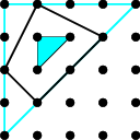
That means, if we move all the edges of $Q=P^{(1)}$ out by one, we obtain a superset $Q^{(-1)}$ of $P$ .

Proof.

We may apply a lattice equivalence to reduce to the case where the edge is defined by $x_{2}\leq 0$ , and that $(0,0)^{t}$ and $(1,0)^{t}$ are two lattice points of $P^{(1)}$ lying on this edge. Suppose indirectly that $P$ has a vertex $\mathbf{v}$ with $v_{2}>1$ . Then the triangle formed by the three points has area $v_{2}/2\geq 1$ . It must therefore contain another lattice point which lies in the interior of $P$ , and has positive second coordinate. ∎

For arbitrary $Q$ , this $Q^{(-1)}$ does not necessarily have integral vertices. But then, not every polygon arises as $P^{(1)}$ for some $P$ . A necessary condition is that the polygon has good angles.

Lemma 9.

If $P^{(1)}$ is $2$ –dimensional, then for all vertices $\mathbf{v}$ of $P^{(1)}$ , the cones generated by $P^{(1)}-\mathbf{v}$ are lattice equivalent to a cone generated by $(1,0)^{t}$ and $(-1,k)^{t}$ , for some integer $k\geq 1$ .

Proof.

Assume, after a lattice equivalence, that $\mathbf{v}=\mathbf{0}$ , and the rays of the cone in question are generated by $(1,0)^{t}$ and $(-p,q)^{t}$ , with coprime $0<p\leq q$ (see Exercise 2). By Lemma 8, all points of $P$ satisfy $x_{2}\geq-1$ and $qx_{1}+px_{2}\geq-1$ . But this implies $x_{1}+x_{2}\geq-1+\frac{p-1}{q}$ . So, if $p>1$ , because $P$ has integral vertices, we have $x_{1}+x_{2}\geq 0$ for all points of $P$ . This contradicts the fact that $\mathbf{0}\in P^{(1)}$ . ∎

For a vertex $\mathbf{v}$ of a polygon define the shifted vertex $\mathbf{v}^{(-1)}$ as follows. Let $\langle\mathbf{a},\mathbf{x}\rangle\leq b$ and $\langle\mathbf{a}^{\prime},\mathbf{x}\rangle\leq b^{\prime}$ be the two edges that intersect in $\mathbf{v}$ . The unique solution to $\langle\mathbf{a},\mathbf{x}\rangle=b+1$ and $\langle\mathbf{a}^{\prime},\mathbf{x}\rangle=b^{\prime}+1$ is denoted $\mathbf{v}^{(-1)}$ . According to Lemma 9, when we deal with $P^{(1)}$ then $\mathbf{v}^{(-1)}$ is a lattice point. (In the situation of the lemma, it is $(0,-1)^{t}$ .) We obtain a characterization of when $Q=P^{(1)}$ for some $P$ .

Lemma 10.

For a polygon $Q$ , the following are equivalent:

•

$Q=P^{(1)}$ for some polygon $P$ .
•

$Q^{(-1)}$ has integral vertices.

Thus, given $Q$ , the maximal polygon $P$ with $P^{(1)}=Q$ is $P=Q^{(-1)}$ . We will (and can) restrict to this situation when we prove the induction step $\ell\leadsto\ell+1$ for the Onion–Skin Theorem.

Proof.

If $Q^{(-1)}$ has integral vertices, then its interior lattice points span $Q$ . For the converse direction, if $Q=P^{(1)}$ then we claim that

(8)

Q^{(-1)}=\mbox{\rm conv}\{\mathbf{v}^{(-1)}\ :\ \mathbf{v}\text{ vertex of }Q\}\ .

To this end, denote $\mathbf{a_{1}},\ldots,\mathbf{a_{n}}$ and $b_{1},\ldots,b_{n}$ the normal vectors respectively right hand sides of the edges of $Q$ in cyclic order. Also, denote $\mathbf{v}_{1},\ldots,\mathbf{v}_{n}$ the vertices of $Q$ so that edge number $k$ is the segment $[{\mathbf{v_{\text{$k$}}},\mathbf{v_{\text{$k\negthinspace+\negthinspace 1$}}}}]$ ( $k\mod n$ ).

“ $\subseteq$ ”: this inclusion holds for arbitrary $Q$ . For a point $\mathbf{y}\in Q^{(-1)}$ , let $\langle\mathbf{a}_{k},\mathbf{x}\rangle\leq b_{k}$ be an edge of $Q$ that maximizes $\langle\mathbf{a},\mathbf{y}\rangle-b$ over all edges. So if $\langle\mathbf{a}_{k},\mathbf{y}\rangle-b_{k}\leq 0$ then $\mathbf{y}\in Q$ . Otherwise we have

•

$b_{k}\leq\langle\mathbf{a}_{k},\mathbf{y}\rangle\leq b_{k}+1$ ,
•

$\langle\mathbf{a}_{k},\mathbf{y}\rangle-b_{k}\geq\langle\mathbf{a}_{k-1},\mathbf{y}\rangle-b_{k-1}$ , and
•

$\langle\mathbf{a}_{k},\mathbf{y}\rangle-b_{k}\geq\langle\mathbf{a}_{k+1},\mathbf{y}\rangle-b_{k+1}$ ,

which describes (a subset of) the convex hull of $\mathbf{v}_{k},\mathbf{v}_{k}^{(-1)},\mathbf{v}_{k+1},\mathbf{v}_{k+1}^{(-1)}$ .

“ $\supseteq$ ”: For this inclusion we actually use $Q=P^{(1)}$ . Figure 17 shows how Equation (8) can fail in general.

Figure 17. Equation (8) can fail in general.

In our situation, $Q=P^{(1)}$ , and we need to show that $v_{k}^{(-1)}$ satisfies all inequalities $\langle\mathbf{a}_{j},\cdot\rangle\leq b_{j}+1$ for $Q^{(-1)}$ . Our assumption implies that $P$ (and therefore $Q^{(-1)}$ by Lemma 8) contains points $\mathbf{w}_{j}$ with $\langle\mathbf{a}_{j},\mathbf{w}_{j}\rangle=b_{j}+1$ . None of the other edge normals belongs to the cone generated by $\mathbf{a}_{k-1}$ and $\mathbf{a}_{k}$ . So for $j\neq k,k-1$ ,

\begin{array}[]{lcccccc}\text{either }&\langle\mathbf{a}_{j},\mathbf{v}_{k}^{(-1)}\rangle&\leq&\langle\mathbf{a}_{j},\mathbf{w}_{k-1}\rangle&\leq&b_{m}+1,\\ \text{or }&\langle\mathbf{a}_{j},\mathbf{v}_{k}^{(-1)}\rangle&\leq&\langle\mathbf{a}_{j},\mathbf{w}_{k}\rangle&\leq&b_{m}+1&\text{ (or both).}\end{array}

∎

Finally, we can prove the key lemma for our induction step.

Lemma 11.

Let $b^{(1)}$ denote the number of lattice points on the boundary of $P^{(1)}$ . Then $b\leq b^{(1)}+9$ , with equality if and only if $P$ is a multiple of $\Delta$ .

This immediately shows that $b\leq b^{(1)}+9\leq i+9$ if $P^{(1)}$ is $2$ –dimensional.

For the proof, we need a result of B. Poonen and F. Rodriguez-Villegas [8]. Consider a primitive oriented segment $s=[{\mathbf{x},\mathbf{y}}]$ , i.e., $\mathbf{x}$ and $\mathbf{y}$ are the only lattice points $s$ contains. Call $s$ admissible if the triangle $\mbox{\rm conv}(\mathbf{0},\mathbf{x},\mathbf{y})$ contains no other lattice points. Equivalently, $s$ is admissible if the determinant $\operatorname{sign}(s)=\left|\begin{smallmatrix}x_{1}&y_{1}\\ x_{2}&y_{2}\end{smallmatrix}\right|$ is equal to $\pm 1$ . The length of a sequence $(s^{(1)},\ldots,s^{(n)})$ of admissible segments is $\sum\operatorname{sign}(s^{(k)})$ .

The dual of an admissible segment is the unique integral normal vector $\mathbf{a}=\mathbf{a}(s)$ such that $\langle\mathbf{a},\mathbf{x}\rangle=\langle\mathbf{a},\mathbf{y}\rangle=1$ . For a closed polygon with segments $(s^{(1)},\ldots,s^{(n)})$ , the dual polygon walks through the normal vectors $\mathbf{a}(s^{(k)})$ .

Figure 18. A polygon and its dual. Their lengths are

1-1+1+1

respectively

1+2+3+4

Theorem 12 (Poonen and Rodriguez-Villegas [8]).

The sum of the lengths of an admissible polygon and its dual is $12$ times the winding number of the polygon.

Heuristically, the winding number counts how many times a polygon winds around the origin. Dual polygons will have equal winding number. In this article, we will only be concerned with polygons of winding number one.

Figure 19. A polygon of winding number

-2

Proof of Lemma 11.

Let $Q=P^{(1)}$ , and note that by Lemma 8, $P\subseteq Q^{(-1)}$ , and by Lemma 10, $Q^{(-1)}$ has integral vertices. Notice that the number of boundary lattice points of $Q$ is $b^{(1)}$ , and let $b^{\prime}$ be the number of boundary lattice points of $Q^{(-1)}$ . Since $P$ and $Q^{(-1)}$ have the same interior lattice points and $P\subseteq Q^{(-1)}$ , by Pick’s Theorem $Q^{(-1)}$ has at least as many boundary lattice points as $P$ ; in other words, $b^{\prime}\geq b$ .

For each of the vertices $v^{(1)}_{1},\ldots,v^{(1)}_{n}$ of $Q$ there is a corresponding vertex $v_{1},\ldots,v_{n}$ of $Q^{(-1)}$ . Consider the (possibly nonconvex, nonsimple) admissible polygon with vertices $v_{1}-v^{(1)}_{1},\ldots,v_{n}-v^{(1)}_{n}$ . It is admissible because there are no lattice points between $Q$ and $Q^{(-1)}$ . One can think of it as what remains of $Q^{(-1)}$ when $Q$ shrinks to a point. Each segment measures the difference (with the correct sign) between the corresponding edges of $Q^{(-1)}$ and $Q$ . I.e., the length of that polygon is precisely $b^{\prime}-b^{(1)}$ .

Now the dual polygon will walk through the normal vectors of $Q$ . Therefore all segments will count with positive length, and there cannot be less than $3$ . Also, there is a unique one with $3$ segments, which is the dual to $3\Delta$ . Thus $b-b^{(1)}\leq b^{\prime}-b^{(1)}\leq 12-3$ with equality only for multiples of $\Delta$ . ∎

Proof of the Onion–Skin Theorem.

Induction on $\ell$ .

•

For $\ell=1$ , the inequality $b\leq 2i+7$ was proved earlier.
•

For $\ell=4/3$ , we have $i=3$ , and $P\subseteq 4\Delta$ . So $b\leq 12$ .
•

For $\ell=5/3$ , we have $i=6$ , and $P\subseteq 5\Delta$ . So $b\leq 15$ .
•

For $\ell=3/2$ , Lemma 11 reads $b\leq i+8$ which is stronger than what we need.

If $\ell\geq 2$ , we have

	$\displaystyle(2\ell-1)b$	$\displaystyle\leq(2\ell-1)b^{(1)}+9(2\ell-1)$
		$\displaystyle=2b^{(1)}+(2(\ell-1)-1)b^{(1)}+9(2\ell-1)$
		$\displaystyle\leq 2b^{(1)}+2i^{(1)}+9(\ell-1)^{2}-2+9(2\ell-1)$
		$\displaystyle=2i+9\ell^{2}-2$

∎

3.2. Generalizing Scott’s proof

As in Subsection 2.1, we tightly fit $P$ into a box $[0,p^{\prime}]\times[0,p]$ , with $p\leq p^{\prime}$ . Let $q$ and $q^{\prime}$ be the length of the top and bottom edge (see Figure 9). We again apply lattice equivalence transformations such that $p$ is as small as possible, and that $P$ has points on the top and bottom edges with horizontal distance smaller than or equal to $(p-q-q^{\prime})/2$ . Again, we obtain the following inequalities:

(5)		$\displaystyle b\leq q+q^{\prime}+2p$
(6)		$\displaystyle a\geq p(q+q^{\prime})/2$
(7)		$\displaystyle a\geq p(p+q+q^{\prime})/4$

Set $x:=p/\ell$ and $y:=(q+q^{\prime})/\ell$ . Then $x\geq 2$ , because passing to $P^{(1)}$ reduces the height at least by 2.³³ 3 We also have $x\leq 3$ with equality only for multiples of $\Delta$ . From (5) and (6), we get

	$\displaystyle\frac{2\ell b-2a-9\ell^{2}}{\ell^{2}}\leq 2(q+q^{\prime}+2p)/\ell-p(q+q^{\prime})/\ell^{2}-9$
	$\displaystyle=-xy+4x+2y-9,$

and from (5) and (7), we get

	$\displaystyle\frac{4\ell b-4a-18\ell^{2}}{\ell^{2}}\leq 4(q+q^{\prime}+2p)/\ell-p(p+q+q^{\prime})/\ell^{2}-18$
	$\displaystyle=-x^{2}-xy+8x+4y-18.$

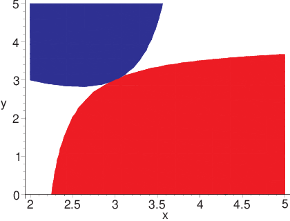
For $x\geq 2$ and $y\geq 0$ , at least one of the two polynomials $p_{1}(x,y)=-xy+4x+2y-9$ and $p_{2}(x,y)=-x^{2}-xy+8x+4y-18$ is zero or negative, as it can be seen in Figure 21. (The two shaded regions are where $p_{1}$ and $p_{2}$ , respectively, take non-negative values.) There is only one point where both upper bounds reach zero, namely $(x,y)=(3,3)$ , and this is the only case where equality can hold in the Onion–Skin Theorem. It is an exercise to show that equality actually holds only for multiples of $\Delta$ .

4. Conclusion

4.1. Summary of results.

For a triple $(a,b,i)$ of numbers the following are equivalent.

•

There is a convex lattice polygon $P$ with $(a,b,i)=(a(P),b(P),i(P))$ .
•
$b\in{\mathbb{Z}}_{\geq 3}$ , $i\in{\mathbb{Z}}_{\geq 0},a=i+b/2-1$ , and
- $\blacktriangleright$
  
  $i=0$ or
- $\blacktriangleright$
  
  $i=1$ and $b\leq 9$ or
- $\blacktriangleright$
  
  $i\geq 2$ and $b\leq 2i+6$ .

Furthermore, if $\ell=\ell(P)$ , then $(2\ell-1)b\leq 2i+9\ell^{2}-2$ .

4.2. Outlook.

Is there a proof of the Onion–Skin Theorem using algebraic geometry? Currently not (yet). The toric dictionary between polygons and algebraic varieties also does not (yet) have an algebraic geometry term for the level of a polygon. A first step in this direction is the use of the process of peeling off onion skins – or rather its algebraic geometry analogue – for the simplification of the rational parametrization of an algebraic surface [11].

In any case, the Onion–Skin Theorem gives rise to a conjecture in algebraic geometry, namely the inequality $(2\ell-1)d\leq 9\ell^{2}+4\ell(p-1)$ for any rational surface of degree $d$ , sectional genus $p$ , and level $\ell$ . Here the level of an algebraic surface should be defined via the process of peeling mentioned above. For toric surfaces, the inequality holds by the Onion–Skin Theorem, but for nontoric rational surfaces we do not have a proof (nor a counterexample).

We thank Ricky Pollack for his encouragement to write up this story. We also thank Daniel J. Velleman and two anonymous referees who helped us do so in a comprehensible way.

References

[1] P. del Pezzo. On the surfaces of order $n$ embedded in $n$ -dimensional space. Rend. mat. Palermo, 1:241–271, 1887.
[2] M. Demazure. Sous-groupes algébriques de rang maximum du group de cremona. Ann. Sci. Ecole Norm. Sup., 3:507–588, 1970.
[3] B. Grünbaum and G. C. Shephard. Pick’s theorem. Amer. Math. Monthly, 100:150–161, 1993.
[4] G. Jung. Un’ osservazione sul grado massimo dei sistemi lineari di curve piane algebriche. Annali di Mat., 2:129–130, 1890.
[5] R. Krasauskas. Toric surface patches. In Advances in geometrical algorithms and representations, volume 17, pages 89–113, 2002.
[6] Jeffrey C. Lagarias and Günter M. Ziegler. Bounds for lattice polytopes containing a fixed number of interior points in a sublattice. Canadian J. Math., 43(5):1022–1035, 1991.
[7] Georg Alexander Pick. Geometrisches zur Zahlenlehre. Sitzenber. Lotos (Prague), 19:311–319, 1899.
[8] Bjorn Poonen and Fernando Rodriguez-Villegas. Lattice polygons and the number 12. Amer. Math. Monthly, 107(3):238–250, 2000.
[9] John E. Reeve. On the volume of lattice polyhedra. Proc. London Math. Soc., 7:378–395, 1957.
[10] J. Schicho. A degree bound for the parameterization of a rational surface. J. Pure Appl. Alg., 145:91–105, 1999.
[11] J. Schicho. Simplification of surface parametrizations – a lattice polygon approach. J. Symb. Comp., 36:535–554, 2003.
[12] Paul R. Scott. On convex lattice polygons. Bull. Austral. Math. Soc., 15(3):395–399, 1976.
[13] Richard P. Stanley. The number of faces of a simplicial convex polytope. Adv. in Math., 35(3):236–238, 1980.
[14] B. Sturmfels. Polynomial equations and convex polytopes. Amer. Math. Monthly, 105:907–922, 1998.

Abstract.

0. Introduction

0.1. How it all began

0.2. Lattice polygons

Theorem 1 (Pick’s Formula [7]).

0.3. Lattice equivalence

Exercise 2.

0.4. Why algebraic geometry?

1. Examples

2. Three proofs of 𝐛≤𝟐​𝐢+𝟕\mathbf{b\leq 2i+7}

Proposition 3.

2.1. Scott’s proof

Exercise 4.

2.2. Clipping off vertices

2.3. Algebraic geometry

Theorem 5.

3. Onion skins

Exercise 6.

Onion–Skin Theorem.

3.1. Moving out edges

Lemma 8.

Proof.

Lemma 9.

Proof.

Lemma 10.

Proof.

Lemma 11.

Theorem 12 (Poonen and Rodriguez-Villegas [8]).

Proof of Lemma 11.

Proof of the Onion–Skin Theorem.

3.2. Generalizing Scott’s proof

4. Conclusion

4.1. Summary of results.

4.2. Outlook.

References

2. Three proofs of $\mathbf{b\leq 2i+7}$