In this thesis, we describe how to construct and enumerate magic squares as lattice points inside polyhedral cones using techniques from Algebraic Combinatorics. The main tools of our methods are the Hilbert Poincaré series to enumerate lattice points and the Hilbert bases to generate lattice points. With these techniques, we derive formulas for the number of magic squares of order 4. We extend Halleck’s work on Pandiagonal squares and Bona’s work on magic cubes and provide formulas for $5\times 5$ pandiagonal squares and $3\times 3\times 3$ magic cubes and semi-magic cubes.

Benjamin Franklin constructed three famous squares which have several interesting properties. Many people have tried to understand the method Franklin used to construct his squares (called Franklin squares) and many theories have been developed along these lines. Our method is a new method to construct not only the three famous squares but all other Franklin squares. We provide formulas for counting the number of Franklin squares and also describe several symmetries of Franklin squares.

Magic labelings of graphs are studied in great detail by Stanley and Stewart. Our methods enable us to construct and enumerate magic labelings of graphs as well. We explore further the correspondence of magic labelings of graphs and symmetric magic squares. We define polytopes of magic labelings of graphs and digraphs, and give a description of the faces of the Birkhoff polytope as polytopes of magic labelings of digraphs.

ACKNOWLEDGMENTS

I take this opportunity to thank my advisor Jesús De Loera for many many things. It was his efforts that secured me admissions to UC Davis and helped me pursue my doctorate degree. He began by teaching me to ace exams and gradually taught me to solve seemingly impossible research problems. I thank him for being an excellent teacher who can make difficult topics easy to understand. I thank him for introducing me to a lot of wonderful mathematics especially algebraic combinatorics. I also thank him for his exceptionally high standards though it was daunting at times. The list is long, so I will just say thanks for making me the mathematician I am today.

I also take this opportunity to thank all the teachers who have had a substantial influence in my mathematical training. I thank Parvati Subramaniam from S.I.E.S high school who was the first teacher I met who could teach mathematics. She made mathematics easy for me and it always stayed easy after-wards. I thank Edward Curtis from University of Washington for making me an Algebra fanatic with the excellent summer course he taught. I thank Ronald Irving at University of Washington for launching my research career. He gave me the necessary confidence with all his encouragement and enthusiasm. I thank Bernd Sturmfels at UC Berkeley from whom I learned Computational Algebraic Geometry and also the thrill of real modern mathematics. His influence is present in all my work.

Its my great pleasure to thank the people at UC Davis for making my stay here memorable. I thank Craig Tracy for all the excellent courses he taught. Craig Tracy always found topics that felt like it was tailor-made for each student in the class. I understand a lot of combinatorics because of him. I thank Abigail Thompson and Motohico Mulase for their timely encouragement. A special thanks to Joel Hass, Matthew Franklin, and Anne Schilling for making my oral exam a pleasant experience. I also thank Greg Kuperberg and Alexander Shoshnikov for their help. In fact, I thank everyone at UC Davis for being so friendly.

I thank my coauthor Raymond Hemmecke from whom I have learned a lot of good mathematics. A special thanks to my officemate Lipika Deka for all the good times and my friend Ruchira Dutta for all her useful comments on my thesis work. I thank my colleague Ruriko Yoshida for help with the program LattE.

I thank my wonderful family: my father Neeliyara Devasia for being the kindest soul on earth; my mother Mariakutty Devasia for all her hard work; my elder brother Santosh Devasia for always being there for me; my younger brother Vinod Devasia for all the good cheer; my sisters-in-law Jessy and Blossom for being nice, my niece Lovita and nephew Brian for just being fun; my in-laws, the Ahmed family: Shafi, Sofia, Shabbir, Juzar, Cynthia, Jasmine, Alicia, and Mohammed for all their help and good times; and finally, my husband Mohsin Ahmed for being my best friend, my guardian angel, my greatest critique, and my all time sponsor¹¹ 1 Partially supported by NSF grant 0309694 and 0073815..

I can no other answer make but thanks,
And thanks; and ever thanks; and oft good turns
Are shuffled off with such uncurrent pay:
But, were my worth as is my conscience firm,
You should find better dealing.
– William Shakespeare.

Foreword

This thesis is a story of fusion of classical mathematics and modern computational mathematics. We redefine the methods of solving classical problems like constructing a magic square and exhibit the power of computational Algebra. For example, only three Franklin squares were known since such squares were difficult to construct. Our results make it possible to construct any number of Franklin squares easily. A detailed description of our methods is given in Section 1.2. More significantly, our study leads to an elegant description of the faces of the Birkhoff polytope as polytopes of magic labelings of digraphs. The main theorems are introduced in Chapter 1 and the subsequent chapters explore the details of these results.

This thesis is based on my three papers

•

Polyhedral cones of magic cubes and squares (joint work with J. De Loera and R. Hemmecke) [2];
•

How many squares are there, Mr. Franklin?: Constructing and Enumerating Franklin Squares [3];
•

Magic graphs and the faces of the Birkhoff polytope [4].

Chapter 1 Introduction

1.1 Magic Squares.

Miracles seem very wonderful to the people who witness them, and very simple to the people who perform them. That does not matter: if they confirm or create faith they are true miracles.

– George Bernard Shaw.

A magic square is a square matrix whose entries are nonnegative integers, such that the sum of the numbers in every row, in every column, and in each diagonal is the same number called the magic sum. The study of magic squares probably dates back to prehistoric times [7]. The Loh-Shu magic square is the oldest known magic square and its invention is attributed to Fuh-Hi (2858-2738 B.C.), the mythical founder of the Chinese civilization [7]. The odd numbers are expressed by white dots, i.e., yang symbols, the emblem of heaven, while the even numbers are in black dots, i.e., yin symbols, the emblem of earth (see Figures 1.1 and 1.2 A).

Refer to caption — Figure 1.1: The Loh-Shu magic square [7].

Like chess and many of the problems founded on the figure of the chess-board, the problem of constructing a magic square probably traces its origin to India [52]. A $4\times 4$ magic square is found in a Jaina inscription of the twelfth or thirteenth century in the city of Khajuraho, India (see Figure 1.2 B). This square shows an advanced knowledge of magic squares because all the pandiagonals also add to the common magic sum (see Figure 1.4).

From India, the problem found its way among the Arabs, and by them it was brought to the Roman Orient. It is recorded that as early as the ninth century magic squares were used by Arabian astrologers in their calculations of horoscopes etc. which might be the reason such squares are called “magic” [7]. Their introduction into Europe appears to have been due to Moschopulus, who lived in Constantinople in the early part of the fifteenth century. The famous Cornelius Agrippa (1486-1535) constructed magic squares of the orders 3, 4, 5, 6, 7, 8, 9, which were associated by him with the seven astrological “planets”; namely, Saturn, Jupiter, Mars, the Sun, Venus, Mercury, and the Moon. A magic square engraved on a silver plate was sometimes prescribed as a charm against the plague and a magic square appears in a well known 1514 engraving by Albrecht Dürer entitled Melancholia (see Figures 1.2 C and 1.3). Magic squares, in general, were considered as mystical objects with the power to ward off evil and bring good fortune. The mathematical theory of the construction of these squares was taken up in France only in the seventeenth century, and since then it has remained a favorite topic of study throughout the mathematical world. See [7], [9], [48], or [52] to read more about the history of magic squares.

Constructing and enumerating magic squares are the two fundamental problems in the topic of magic squares. Let $M_{n}(s)$ denote the number of $n\times n$ magic squares of magic sum $s$ . In 1906, MacMahon [43] enumerated magic squares of order 3:

M_{3}(s)=\left\{\begin{array}[]{ll}{\frac{2}{9}}s^{2}+{\frac{2}{3}}s+1&\mbox{if 3 divides $s$},\\ 0&\mbox{otherwise.}\end{array}\right.

Later, MacMahon [43], Anand et al. [6], and Stanley [54], considered the problem of enumerating semi-magic squares which are squares such that only the row and column sums add to a magic sum (see [54]).

In this thesis, we have used methods from algebra, combinatorics, and polyhedral geometry to construct and enumerate magic squares and these methods are similar to the methods used by Stanley to enumerate semi-magic squares [54]. Part of our work is based on generalizing his ideas. Polyhedral methods were also used by Halleck in his 2000 Ph.D thesis (see [37]) and Beck et al. in [12] to enumerate various kinds of magic squares. Our techniques are different and are more algebraic in flavor.

The basic idea is to consider the defining linear equations of magic squares. These equations, together with the nonnegativity requirement on the entries, imply that the set of magic squares becomes the set of integral points inside a pointed polyhedral cone (see [2] or [53]). The minimal Hilbert basis of this cone is defined to be the smallest finite set $S$ of integral points with the property that any integral point can be expressed as a linear combination with nonnegative integer coefficients of the elements of $S$ [51]. For example, the minimal Hilbert basis of the $3\times 3$ magic squares is given in Figure 1.5 and a Hilbert basis construction of the Loh-shu magic square is given in Figure 1.6.

We map magic squares to monomials in a polynomial ring to enumerate them and derive the formula for the number of $4\times 4$ magic squares of magic sum $s$ (also derived simultaneously by Beck et al. [12] using different techniques).

Theorem 1.1.1.

The number of $4\times 4$ magic squares with magic sum $s$ ,

M_{4}(s)=\left\{\begin{array}[]{l}\frac{1}{480}s^{7}+\frac{7}{240}s^{6}+\frac{89}{480}s^{5}+\frac{11}{16}s^{4}+\frac{779}{480}s^{3}+\frac{593}{240}s^{2}+\frac{1051}{480}s+\frac{13}{16},\\ \\ \hfill\mbox{when $s$ is odd},\\ \\ \\ \frac{1}{480}s^{7}+\frac{7}{240}s^{6}+\frac{89}{480}s^{5}+\frac{11}{16}s^{4}+\frac{49}{30}s^{3}+\frac{38}{15}s^{2}+\frac{71}{30}s+1,\\ \\ \hfill\mbox{ when $s$ is even.}\end{array}\right.

We will describe this method in detail in the next section (also, see [2] and [3]).

1.2 Generating and enumerating lattice points inside polyhedral cones.

In this section we illustrate the algebraic techniques of generating and enumerating lattice points inside polyhedral cones by applying the method to construct and enumerate magic squares. As an example, we walk through the details of the proof of Theorem 1.1.1.

For these purposes we regard $n\times n$ magic squares as either $n\times n$ matrices or vectors in $\mathbb{R}^{n^{2}}$ and apply the normal algebraic operations to them. We also consider the entries of an $n\times n$ magic square as variables $y_{ij}\hskip 3.61371pt(1\leq i,j\leq n)$ . If we set the first row sum equal to all other mandatory sums, then magic squares become nonnegative integral solutions to a system of linear equations $Ay=0$ , where $A$ is an $(2n+1)\times n^{2}$ matrix each of whose entries is 0, 1, or -1.

For example, the equations defining $3\times 3$ magic squares are:

\begin{array}[]{c}y_{11}+y_{12}+y_{13}=y_{21}+y_{22}+y_{23}\\ y_{11}+y_{12}+y_{13}=y_{31}+y_{32}+y_{33}\\ y_{11}+y_{12}+y_{13}=y_{11}+y_{21}+y_{31}\\ y_{11}+y_{12}+y_{13}=y_{12}+y_{22}+y_{32}\\ y_{11}+y_{12}+y_{13}=y_{13}+y_{23}+y_{33}\\ y_{11}+y_{12}+y_{13}=y_{11}+y_{22}+y_{33}\\ y_{11}+y_{12}+y_{13}=y_{13}+y_{22}+y_{31}\end{array}

Therefore, $3\times 3$ magic squares are nonnegative integer solutions to the system of equations $Ay=0$ where:

\begin{array}[]{lll}A=\left[\begin{array}[]{rrrrrrrrr}1&1&1&-1&-1&-1&0&0&0\\ 1&1&1&0&0&0&-1&-1&-1\\ 0&1&1&-1&0&0&-1&0&0\\ 1&0&1&0&-1&0&0&-1&0\\ 1&1&0&0&0&-1&0&0&-1\\ 0&1&1&0&-1&0&0&0&-1\\ 1&1&0&0&-1&0&-1&0&0\\ \end{array}\right]&\mbox{and}&y=\left[\begin{array}[]{r}y_{11}\\ y_{12}\\ y_{13}\\ y_{21}\\ y_{22}\\ y_{23}\\ y_{31}\\ y_{32}\\ y_{33}\end{array}\right]\end{array}

A nonempty set $C$ of points in $\mathbb{R}^{n^{2}}$ is a cone if $au+bv$ belongs to $C$ whenever $u$ and $v$ are elements of $C$ and $a$ and $b$ are nonnegative real numbers. A cone is pointed if the origin is its only vertex (or minimal face; see [51]). A cone $C$ is polyhedral if $C=\{y:Ay\leq 0\}$ for some matrix $A$ , i.e, if $C$ is the intersection of finitely many half-spaces. If, in addition, the entries of the matrix $A$ are rational numbers, then $C$ is called a rational polyhedral cone. A point $y$ in the cone $C$ is called an integral point if all its coordinates are integers.

It is easy to verify that the sum of two magic squares is a magic square and that nonnegative integer multiples of magic squares are magic squares. Therefore, the set of magic squares is the set of all integral points inside a polyhedral cone $C_{M_{n}}=\{y:Ay=0,y\geq 0\}$ in $\mathbb{R}^{n^{2}}$ , where $A$ is the coefficient matrix of the defining linear system of equations. Observe that $C_{M_{n}}$ is a pointed cone.

In the example of $4\times 4$ magic squares, there are three linear relations equating the first row sum to all other row sums and four more equating the first row sum to column sums. Similarly, equating the two diagonal sums to the first row sum generates two more linear equations. Thus, there are a total of 9 linear equations that define the cone of $4\times 4$ magic squares. The coefficient matrix $A$ has rank 8 and therefore the cone $C_{M_{4}}$ of $4\times 4$ magic squares has dimension $16-8=8$ (see [51]).

In 1979, Giles and Pulleyblank introduced the notion of a Hilbert basis of a cone [34]. For a given cone $C$ , its set $S_{C}=C\cap{\mathbb{Z}}^{n}$ of integral points is called the semigroup of the cone $C$ .

Definition 1.2.1.

A Hilbert basis for a cone $C$ is a finite set of points $HB(C)$ in its semigroup $S_{C}$ such that each element of $S_{C}$ is a linear combination of elements from $HB(C)$ with nonnegative integer coefficients.

For example, the integral points inside and on the boundary of the parallelepiped in $\mathbb{R}^{2}$ with vertices $(0,0),(3,2),(1,3)$ and $(4,5)$ in Figure 1.7 form a Hilbert basis of the cone generated by the vectors $(1,3)$ and $(3,2)$ .

We recall an important fact about Hilbert bases [51, Theorem 16.4]:

Theorem 1.2.1.

Each rational polyhedral cone $C$ is generated by a Hilbert basis. If $C$ is pointed, then there is a unique minimal integral Hilbert basis generating $C$ (minimal relative to taking subsets).

We present a proof of Theorem 1.2.1 in Appendix A. The minimal Hilbert basis of a pointed cone is unique and henceforth, when we say the Hilbert basis, we mean the minimal Hilbert basis. An integral point of a cone $C$ is irreducible if it is not a linear combination with integer coefficients of other integral points. All the elements of the minimal Hilbert basis are irreducible [38], [51]. Since magic squares are integral points inside a cone, Theorem 1.2.1 implies that every magic square is a nonnegative integer linear combination of irreducible magic squares.

The minimal Hilbert basis of the polyhedral cone of $4\times 4$ magic squares is given in Figure 1.8 and was computed using the software MLP (now called 4ti2) (see [38]; software implementation 4ti2 is available from http://www.4ti2.de). In fact, all Hilbert basis calculations in this thesis are done with the software 4ti2.

Hilbert basis constructions of the Jaina, and the Dürer magic squares are given in Figures 1.9 and 1.10 respectively.

Different combinations of the elements of a Hilbert basis sometimes produce the same magic square. Figures 1.9 and 1.11 exhibit two different Hilbert basis constructions of the Jaina magic square. This is due to algebraic dependencies among the elements of the Hilbert basis. Repetitions have to be avoided when counting squares, a problem that we solve by using a little bit of commutative algebra. Let $HB(C_{M_{n}})=\{h_{1},h_{2},\dots h_{r}\}$ be a Hilbert basis for the cone of $n\times n$ magic squares. Denote the entries of the square $h_{p}$ by $y^{p}_{ij}$ , and let $k$ be any field. Let $\phi$ be the unique ring homomorphism between the polynomial rings $k[x_{1},x_{2},\dots,x_{r}]$ and $k[t_{11},t_{12},\dots,t_{1n},t_{21},t_{22},\dots t_{2n},\dots,t_{n1},t_{n2},\dots,t_{nn}]$ such that $\phi(x_{p})=t^{h_{p}}$ , the monomial defined by

t^{h_{p}}=\prod_{i,j=1,\dots,n}t_{ij}^{y^{p}_{ij}}.

Monomials in $k[x_{1},x_{2},\dots,x_{r}]$ correspond to magic squares under this map, and multiplication of monomials corresponds to addition of magic squares. For example, the monomial $x_{1}^{5}x_{3}^{200}$ corresponds to the magic square $5h_{1}+200h_{3}$ . Different combinations of Hilbert basis elements that give rise to the same magic square can then be represented as polynomial equations. Thus, from the two different Hilbert basis constructions of the Jaina magic square represented in Figures 1.9 and 1.11, we learn that

\begin{array}[]{l}h1+4\cdot h3+2\cdot h4+8\cdot h5+3\cdot h6+12\cdot h7+4\cdot h8=\\ h3+8\cdot h5+h6+11\cdot h7+h8+h14+2\cdot h15+2\cdot h17+h20\end{array}

In $k[x_{1},x_{2},\dots,x_{r}]$ , this algebraic dependency of Hilbert basis elements translates to

\begin{array}[]{l}x_{1}x_{3}^{4}x_{4}^{2}x_{5}^{8}x_{6}^{3}x_{7}^{12}x_{8}^{4}-x_{3}x_{5}^{8}x_{6}x_{7}^{11}x_{8}x_{14}x_{15}^{2}x_{17}^{2}x_{20}=0.\end{array}

Consider the set of all polynomials in $k[x_{1},x_{2},\dots,x_{r}]$ that are mapped to the zero polynomial under $\phi$ . This set, which corresponds to all the algebraic dependencies of Hilbert basis elements, forms an ideal in $k[x_{1},x_{2},\dots,x_{r}]$ , an ideal known as the toric ideal of $HB(C_{M_{n}})$ (see [2], [14], or [59] for details about toric ideals). If we denote the toric ideal as $I_{HB(C_{M_{n}})}$ , then the monomials in the quotient ring $R_{C_{M_{n}}}=k[x_{1},x_{2},\cdots,x_{r}]/I_{HB(C_{M_{n}})}$ are in one-to-one correspondence with magic squares.

For example, in the case of $3\times 3$ magic squares, there are 5 Hilbert basis elements (see Figure 1.5) and hence there are 5 variables $x_{1},x_{2},x_{3},x_{4},x_{5}$ which gets mapped by $\phi$ as follows:

\begin{array}[]{cccc}x_{1}\mapsto&\left[\begin{array}[]{ccc}1&0&2\\ 2&1&0\\ 0&2&1\end{array}\right]\mapsto&t_{11}{t_{13}}^{2}{t_{21}}^{2}t_{22}{t_{32}}^{2}t_{33}\\ \\ x_{2}\mapsto&\left[\begin{array}[]{ccc}2&0&1\\ 0&1&2\\ 1&2&0\end{array}\right]\par\mapsto&{t_{11}}^{2}t_{13}t_{22}{t_{23}}^{2}t_{31}{t_{32}}^{2}\\ \\ x_{3}\mapsto&\left[\begin{array}[]{ccc}0&2&1\\ 2&1&0\\ 1&0&2\end{array}\right]\mapsto&{t_{12}}^{2}t_{13}{t_{21}}^{2}t_{22}t_{31}{t_{33}}^{2}\\ \\ x_{4}\mapsto&\left[\begin{array}[]{ccc}1&2&0\\ 0&1&2\\ 2&0&1\end{array}\right]\mapsto&t_{11}{t_{12}}^{2}t_{22}{t_{23}}^{2}{t_{31}}^{2}t_{33}\\ \\ x_{5}\mapsto&\left[\begin{array}[]{ccc}1&1&1\\ 1&1&1\\ 1&1&1\end{array}\right]\mapsto&t_{11}t_{12}t_{13}t_{21}t_{22}t_{23}t_{31}t_{32}t_{33}\par\end{array}

We use CoCoA to compute the toric ideal

I_{HB(C_{M_{3}})}=(x_{1}x_{4}-x_{5}^{2},x_{2}x_{3}-x_{1}x_{4}).

Thus

R_{C_{M_{3}}}=\frac{Q[x_{1},x_{2},x_{3},x_{4},x_{5}]}{(x_{1}x_{4}-x_{5}^{2},x_{2}x_{3}-x_{1}x_{4})}.

Let $R_{C_{M_{n}}}(s)$ be the set of all homogeneous polynomials of degree $s$ in the ring $R_{C_{M_{n}}}$ . Then $R_{C_{M_{n}}}(s)$ is a $k$ -vector space, and $R_{C_{M_{n}}}(0)=k$ . The dimension $\mbox{dim}_{k}(R_{C_{M_{n}}}(s))$ of $R_{C_{M_{n}}}(s)$ is precisely the number of monomials of degree $s$ in $R_{C_{M_{n}}}$ .

Recall that if the variables $x_{i}$ of a polynomial ring $k[x_{1},x_{2},\dots,x_{r}]$ are assigned nonnegative weights $w_{i}$ , then the weighted degree of a monomial $x_{1}^{\alpha_{1}}\cdots x_{r}^{\alpha_{r}}$ is $\sum_{i=1}^{r}\alpha_{i}\cdot w_{i}$ (see [8]). Therefore, if we take the weight of the variable $x_{i}$ to be the magic sum of the corresponding Hilbert basis element $h_{i}$ , then $\mbox{dim}_{k}(R_{C_{M_{n}}}(s))$ is exactly the number of magic squares of magic sum $s$ . For example, in the case of $3\times 3$ magic squares, because all the elements of the Hilbert basis have sum 3, all the variables are assigned degree 3.

Since $R_{C_{M_{n}}}$ is a graded $k$ -algebra, it can be decomposed into a direct sum of its graded components $R_{C_{M_{n}}}=\bigoplus R_{C_{M_{n}}}(s)$ (see [2] or [8]). Consider a finitely generated graded $k$ -algebra $R_{C_{M_{n}}}=\bigoplus R_{C_{M_{n}}}(s)$ . The function $H(R_{C_{M_{n}}},s)=\mbox{dim}_{k}(R_{C_{M_{n}}}(s))$ is the Hilbert function of $R_{C_{M_{n}}}$ and the Hilbert-Poincaré series of $R_{C_{M_{n}}}$ is the formal power series

H_{R_{C_{M_{n}}}}(t)=\sum_{s=0}^{\infty}H(R_{C_{M_{n}}},s)t^{s}.

We can now deduce the following lemma.

Lemma 1.2.1.

Let the weight of a variable $x_{i}$ in the ring $R=k[x_{1},x_{2},...,x_{r}]$ be the magic sum of the corresponding element of the Hilbert basis $h_{i}$ . With this grading of degrees on the monomials of $R$ , the number of distinct magic squares of magic sum $s$ is given by the value of the Hilbert function $H(R_{C_{M_{n}}},s)$ .

We record here a version of the Hilbert-Serre Theorem. A proof of the Hilbert-Serre theorem in all its generality is presented in Appendix A.

Theorem 1.2.2 (Theorem 11.1 [8]).

Let $k$ be a field and $R:=k[x_{1},x_{2},...,x_{r}]$ be a graded Noetherian ring. let $x_{1},x_{2},...,x_{r}$ be homogeneous of degrees $>0$ . Let $M$ be a finitely generated $R$ -module. Then the Hilbert Poincaré series of $M$ , $H_{M}(t)$ is a rational function of the form:

H_{M}(t)=\frac{p(t)}{\Pi_{i=1}^{r}(1-t^{degx_{i}})},

where $p(t)\in{\mathbb{Z}}[t]$ .

By invoking the Hilbert-Serre theorem, we conclude that the Hilbert-Poincaré series is a rational function of the form $H_{R_{C_{M_{n}}}}(t)={p(t)}/{\Pi_{i=1}^{r}(1-t^{degx_{i}})}$ , where $p(t)$ belongs to ${\mathbb{Z}}[t]$ . We refer the reader to [2], [8], [15], or [53] for information about Hilbert-Poincaré series.

We can also arrive at the conclusion that $H_{R_{C_{M_{n}}}}(t)$ is a rational function by studying rational polytopes. A polytope $\cal P$ is called rational if each vertex of $\cal P$ has rational coordinates. The dilation of a polytope ${\cal P}$ by an integer $s$ is defined to be the polytope $s{\cal P}=\{s{\alpha}:{\alpha}\in{\cal P}\}$ (see Figure 1.12 for an example).

Let $i({\cal P},s)$ denote the number of integer points inside the polytope $s{\cal P}$ . If ${\alpha\in{\mathbb{Q}}^{m}}$ , let den ${\alpha}$ be the least positive integer $q$ such that $q{\alpha}\in{\mathbb{Z}}^{m}$ .

Theorem 1.2.3 (Theorem 4.6.25 [53]).

Let $\cal P$ be a rational convex polytope of dimension $d$ in ${\mathbb{R}}^{m}$ with vertex set $V$ . Set $F({\cal P},t)=1+{\sum}_{n\geq 1}i({\cal P},s)t^{s}$ . Then $F({\cal P},t)$ is a rational function, which can be written with denominator ${\prod}_{{\alpha}\in V}(1-t^{\mbox{den }{\alpha}})$ .

To extract explicit formulas from the generating function we need to define the concept of quasi-polynomials.

Definition 1.2.2.

A function $f:{\mathbb{N}}\mapsto{\mathbb{C}}$ is a quasi-polynomial if there exists an integer $N>0$ and polynomials $f_{0},f_{1},...,f_{d}$ such that

\begin{array}[]{ll}f(n)=f_{i}(n)&if\ n\equiv i(\mbox{mod}N).\end{array}

The integer $N$ is called a quasi-period of $f$ .

For example, the formula for the number of $3\times 3$ magic squares of magic sum $s$ is a quasi-polynomial with quasi-period 3 (see Section 1.1). We now state some properties of quasi-polynomials.

Proposition 1.2.1 (Corollary 4.3.1 [53]).

The following conditions on a function $f:{\mathbb{N}}\mapsto{\mathbb{C}}$ and integer $N>0$ are equivalent:

1.

$f$ is a quasi-polynomial of quasi-period $N$ .
2.

${\sum}_{n\geq 0}f(n)x^{n}=\frac{P(x)}{Q(x)}$ ,

where $P(x)$ and $Q(x)\in{\mathbb{C}}[x]$ , every zero $\alpha$ of $Q(x)$ satisfies ${\alpha}^{N}=1$ (provided ${P(x)}/{Q(x)}$ has been reduced to lowest terms) and deg $P<$ deg $Q$ .
3.

For all $n\geq 0$ ,

$f(n)={\sum}_{i=1}^{k}P_{i}(n){\gamma}_{i}^{n}$

where each $P_{i}$ is a polynomial function of $n$ and each ${\gamma}_{i}$ satisfies ${\gamma}_{i}^{N}=1.$ The degree of $P_{i}(n)$ is one less than the multiplicity of the root ${\gamma}_{i}^{-1}$ in ${Q(x)}$ provided ${P(x)}/{Q(x)}$ has been reduced to lowest terms.

Theorem 1.2.3 together with Proposition 1.2.1 imply that $i({\cal P},s)$ is a quasi-polynomial and is generally called the Ehrhart quasi-polynomial of $\cal P$ . A polytope is called an integral polytope when all its vertices have integral coordinates. $i({\cal P},s)$ is a polynomial if $\cal P$ is an integral polytope [53].

The convex hull of $n\times n$ matrices, with nonnegative real entries, such that all the row sums, the column sums, and the diagonal sums equal $1$ , is called the polytope of stochastic magic squares. Then, clearly $M_{n}(s)$ is the Ehrhart quasi-polynomial of the polytope of stochastic magic squares. Therefore, by Theorem 1.2.3, we get, again, that $H_{R_{C_{M_{n}}}}(t)$ is a rational function.

Coming back to the case of $4\times 4$ magic squares, we used the program CoCoA (see [21]; CoCoA software is available from http://cocoa.dima.unige.it) to compute the Hilbert-Poincaré series $\sum_{s=0}^{\infty}M_{4}(s)t^{s}$ and obtained

\begin{array}[]{l}\sum_{s=0}^{\infty}M_{4}(s)t^{s}=\frac{t^{8}+4t^{7}+18t^{6}+36t^{5}+50t^{4}+36t^{3}+18t^{2}+4t+1}{(1-t)^{4}(1-t^{2})^{4}}=\\ \\ 1+8t+48t^{2}+200t^{3}+675t^{4}+1904t^{5}+4736t^{6}+10608t^{7}+21925t^{8}+\ldots\end{array}

Recall that the coefficient of $t^{s}$ is the number of magic squares of magic sum $s$ . This information along with Proposition 1.2.1 enables us to recover the Hilbert function $M_{4}(s)$ in Theorem 1.1.1 from the Hilbert-Poincaré series by interpolation. We provide basic algorithms to compute Hilbert bases, toric ideals, and Hilbert-Poincaré series in Appendix B.

We can also study magic figures of higher dimensions with our methods. Similar enumerative results for magic cubes and further properties of the associated cones are discussed in Chapter 2. See Figure 1.13 for a Hilbert basis construction of a magic cube.

In the next section we apply these methods to construct and enumerate pandiagonal magic squares.

1.3 Pandiagonal magic squares.

We continue the the study of pandiagonal magic squares started in [1, 37]. Here we investigate the Hilbert bases, and recompute the formulas of Halleck (computed using a different method, see [37, Chapters 8 and 10]).

The convex hull of $n\times n$ matrices, with nonnegative real entries, such that all the row sums, the column sums, and the pandiagonal sums equal $1$ , is called the polytope of panstochastic magic squares. The integrality of the polytope of panstochastic magic squares was fully solved in [1].

Let us denote by $MP_{n}(s)$ the number of $n\times n$ pandiagonal magic squares with magic sum $s$ . Halleck [37] computed the dimension of the cone to be $(n-2)^{2}$ for odd $n$ and $(n-2)^{2}+1$ for even $n$ (degree of the quasipolynomial $MP_{n}(s)$ is one less than these). For the $4\times 4$ pandiagonal magic squares a fast calculation corroborates that there are 8 elements in the Hilbert basis (see Figure 1.14). In his investigations, Halleck [37] identified a much larger generating set. Recall that the Jaina magic square is also a pandiagonal magic square. A pandiagonal Hilbert basis construction of the Jaina magic square is given in Figure 1.15.

We verify that the $5\times 5$ pandiagonal magic squares have indeed a polynomial counting formula. This case requires in fact no calculations thanks to earlier work by [1] who proved that for $n=5$ the only pandiagonal rays are precisely the pandiagonal permutation matrices. It is easy to see that only 10 of the 120 permutation matrices of order 5 are pandiagonal. A 4ti2 computation shows that the set of pandiagonal permutation matrices is also the Hilbert basis (see Figure 1.16).

We calculate the formulas stated in Theorem 1.3.1 using CoCoA:

Theorem 1.3.1.

MP_{4}(s)=\left\{\begin{array}[]{ll}\frac{1}{48}(s^{2}+4s+12)(s+2)^{2}&\mbox{if $2$ divides $s$,}\\ 0&\mbox{otherwise.}\cr\end{array}\right.

MP_{5}(s)=\frac{1}{8064}(s+4)(s+3)(s+2)(s+1)(s^{2}+5s+8)(s^{2}+5s+42).

In the next section, we apply our methods to study Franklin squares which are more complex than the squares we have seen so far.

1.4 Franklin Squares.

The well-known squares F1 and F3, as well as the less familiar F2, that appear in Figure 1.17 were constructed by Benjamin Franklin (see [7] and [45]). In a letter to Peter Collinson (see [7]) he describes the properties of the $8\times 8$ square F1 as follows:

1.

The entries of every row and column add to a common sum called the magic sum.
2.

In every half-row and half-column the entries add to half the magic sum.
3.

The entries of the main bent diagonals (see Figure 1.19) and all the bent diagonals parallel to it (see Figure 1.20) add to the magic sum.
4.

The four corner entries together with the four middle entries add to the magic sum.

Henceforth, when we say row sum, column sum, bent diagonal sum, and so forth, we mean that we are adding the entries in the corresponding configurations. Franklin mentions that the square F1 has five other curious properties but fails to list them. He also says, in the same letter, that the $16\times 16$ square F3 has all the properties of the $8\times 8$ square, but that in addition, every $4\times 4$ subsquare adds to the common magic sum. More is true about this square F3. Observe that every $2\times 2$ subsquare in F3 adds to one-fourth the magic sum. The $8\times 8$ squares have magic sum 260 while the $16\times 16$ square has magic sum 2056. For a detailed study of these three “Franklin” squares, see [7], [45], or [46].

We define $8\times 8$ Franklin squares to be squares with nonnegative integer entries that have the properties (1) - (4) listed by Benjamin Franklin and the additional property that every $2\times 2$ subsquare adds to one-half the magic sum (see Figure 1.18). The $8\times 8$ squares constructed by Franklin have this extra property (this might be one of the unstated curious properties to which Franklin was alluding in his letter). It is worth noticing that the fourth property listed by Benjamin Franklin becomes redundant with the assumption of this additional property.

Similarly, we define $16\times 16$ Franklin squares to be $16\times 16$ squares that have nonnegative integer entries with the property that all rows, columns, and bent diagonals add to the magic sum, the half-rows and half-columns add to one-half the magic sum, and the $2\times 2$ subsquares add to one-fourth the magic sum. The $2\times 2$ subsquare property implies that every $4\times 4$ subsquare adds to the common magic sum.

The property of the $2\times 2$ subsquares adding to a common sum and the property of bent diagonals adding to the magic sum are “continuous properties.” By this we mean that, if we imagine the square as the surface of a torus (i.e., if we glue opposite sides of the square together), then the bent diagonals and the $2\times 2$ subsquares can be translated without effect on the corresponding sums (see Figure 1.20).

When the entries of an $n\times n$ Franklin square ( $n=8$ or $n=16$ ) are $1,2,3,\dots,n^{2}$ , it is called a natural Franklin square. Observe that the squares in Figure 1.17 are natural Franklin squares. Very few such squares are known, for the simple reason that squares of this type are difficult to construct. Many authors have looked at the problem of constructing them (see, for example, [7], [45], and [47] and the references therein).

Our method is a new way to construct F1, F2, and F3. We are also able to construct new natural Franklin squares, not isomorphic to the ones previously known. A permutation of the entries of a Franklin square is a symmetry operation if it maps the set of all Franklin squares to itself, and two squares are called isomorphic if it is possible to transform one to the other by applying symmetry operations. We start by describing several symmetries of the Franklin squares.

Theorem 1.4.1.

The following operations on $n\times n$ Franklin squares, where $n=8$ or $n=16$ , are symmetry operations: rotating the square by 90 degrees; reflecting the square across one of its edges; transposing the square; interchanging alternate columns (respectively, rows) $i$ and $i+2$ , where $1\leq i\leq(n/2)-2$ or $(n/2)+1\leq i\leq n-2$ ; interchanging the first $n/2$ columns (respectively, rows) of the square with the last $n/2$ columns (respectively, rows) simultaneously; interchanging all the adjacent columns (respectively, rows) $i$ and $i+1$ $(i=1,3,5,\dots n-1)$ of the square simultaneously.

The following operations are additional symmetry operations on $16\times 16$ Franklin squares: interchanging columns (respectively, rows) $i$ and $i+4$ , where $1\leq i\leq 4$ or $9\leq i\leq 12$ .

The proof of Theorem 1.4.1 is presented in Chapter 3.

The following theorem addresses itself to the squares in Figures 1.17 and 1.22.

Theorem 1.4.2.

The original Franklin squares F1 and F2 are not isomorphic. The squares N1, N2, and N3 are nonisomorphic natural $8\times 8$ Franklin squares that are not isomorphic to either F1 or F2. The square N4 is a natural $16\times 16$ Franklin square that is not isomorphic to square F3.

We give a proof of Theorem 1.4.2 in Chapter 3. We now enumerate Franklin squares with our methods.

Theorem 1.4.3.

Let $F_{8}(s)$ denote the number of $8\times 8$ Franklin squares with magic sum $s$ . Then:

F_{8}(s)=\left\{\begin{array}[]{l}\begin{array}[]{l}{\frac{23}{627056640}}\,{s}^{9}+{\frac{23}{17418240}}\,{s}^{8}+{\frac{167}{6531840}}\,{s}^{7}+{\frac{5}{15552}}\,{s}^{6}+{\frac{2419}{933120}}\,{s}^{5}+{\frac{1013}{77760}}\,{s}^{4}+{\frac{701}{22680}}\,{s}^{3}\\ \\ -{\frac{359}{10206}}\,{s}^{2}-{\frac{177967}{816480}}\,s+{\frac{241}{17496}}\end{array}\\ \hfill\mbox{if s $\equiv 2$ (mod $12$) and $s\neq 2$, }\\ \\ \begin{array}[]{l}{\frac{23}{627056640}}\,{s}^{9}+{\frac{23}{17418240}}\,{s}^{8}+{\frac{167}{6531840}}\,{s}^{7}+{\frac{5}{15552}}\,{s}^{6}+{\frac{581}{186624}}\,{s}^{5}+{\frac{1823}{77760}}\,{s}^{4}+{\frac{6127}{45360}}\,{s}^{3}\\ \\ +{\frac{10741}{20412}}\,{s}^{2}+{\frac{113443}{102060}}\,s+{\frac{3211}{2187}}\end{array}\\ \hfill\mbox{if $s\equiv 4$ (mod $12$),}\\ \\ \begin{array}[]{l}{\frac{23}{627056640}}\,{s}^{9}+{\frac{23}{17418240}}\,{s}^{8}+{\frac{167}{6531840}}\,{s}^{7}+{\frac{5}{15552}}\,{s}^{6}+{\frac{2419}{933120}}\,{s}^{5}+{\frac{1013}{77760}}\,{s}^{4}+{\frac{701}{22680}}\,{s}^{3}\\ \\ -{\frac{5}{378}}\,{s}^{2}-{\frac{3967}{10080}}\,s-{\frac{13}{8}}\end{array}\\ \hfill\mbox{if $s\equiv 6$ (mod $12$),}\\ \\ \begin{array}[]{l}{\frac{23}{627056640}}\,{s}^{9}+{\frac{23}{17418240}}\,{s}^{8}+{\frac{167}{6531840}}\,{s}^{7}+{\frac{5}{15552}}\,{s}^{6}+{\frac{581}{186624}}\,{s}^{5}+{\frac{1823}{77760}}\,{s}^{4}+{\frac{6127}{45360}}\,{s}^{3}\\ \\ +{\frac{11189}{20412}}\,{s}^{2}+{\frac{167203}{102060}}\,s+{\frac{5771}{2187}}\end{array}\\ \hfill\mbox{if $s\equiv 8$ (mod $12$),}\\ \\ \begin{array}[]{l}{\frac{23}{627056640}}\,{s}^{9}+{\frac{23}{17418240}}\,{s}^{8}+{\frac{167}{6531840}}\,{s}^{7}+{\frac{5}{15552}}\,{s}^{6}+{\frac{2419}{933120}}\,{s}^{5}+{\frac{1013}{77760}}\,{s}^{4}+{\frac{701}{22680}}\,{s}^{3}\\ \\ -{\frac{583}{10206}}\,{s}^{2}-{\frac{608047}{816480}}\,s-{\frac{20239}{17496}}\end{array}\\ \hfill\mbox{if $s\equiv 10$ (mod $12$),}\\ \\ \begin{array}[]{l}{\frac{23}{627056640}}\,{s}^{9}+{\frac{23}{17418240}}\,{s}^{8}+{\frac{167}{6531840}}\,{s}^{7}+{\frac{5}{15552}}\,{s}^{6}+{\frac{581}{186624}}\,{s}^{5}+{\frac{1823}{77760}}\,{s}^{4}+{\frac{6127}{45360}}\,{s}^{3}\\ \\ +{\frac{431}{756}}\,{s}^{2}+{\frac{1843}{1260}}\,s+1\end{array}\\ \hfill\mbox{if $s\equiv 0$ (mod $12$),}\\ \\ \begin{array}[]{l}0\end{array}\\ \hfill\mbox{otherwise.}\end{array}\right.

The $8\times 8$ pandiagonal Franklin squares are the $8\times 8$ Franklin squares that have all the pandiagonals adding to the common magic sum (see Figure 1.4). Our techniques enable us to construct and count $8\times 8$ pandiagonal Franklin squares as well:

Theorem 1.4.4.

Let $PF_{8}(s)$ denote the number of $8\times 8$ pandiagonal Franklin squares with magic sum $s$ . Then:

PF_{8}(s)=\left\{\begin{array}[]{l}{\frac{1}{2293760}}{s}^{8}+{\frac{1}{71680}}{s}^{7}+{\frac{1}{3840}}{s}^{6}+{\frac{1}{320}}{s}^{5}+{\frac{1}{40}}{s}^{4}+{\frac{2}{15}}{s}^{3}+{\frac{197}{420}}{s}^{2}+{\frac{106}{105}}s+1\\ \hfill\mbox{if $s\equiv 0$ (mod $4$),}\\ 0\\ \hfill\mbox{otherwise.}\end{array}\right.

We introduce magic graphs and explore its connections to symmetric magic squares in the next section.

1.5 Magic labelings of graphs.

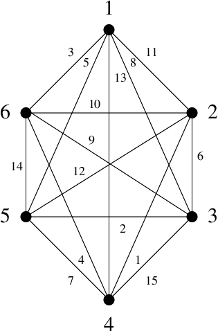
Let $G$ be a finite graph. A labeling of $G$ is an assignment of a nonnegative integer to each edge of $G$ . A magic labeling of magic sum $r$ of $G$ is a labeling such that for each vertex $v$ of $G$ the sum of the labels of all edges incident to $v$ is the magic sum $r$ (loops are counted as incident only once). Graphs with a magic labeling are also called magic graphs (see 1.23 for an example of a magic labeling of the complete graph $K_{6}$ ). Magic graphs are also studied in great detail by Stanley and Stewart in [55], [56], [57], and [58].

We define a magic labeling of a digraph $D$ of magic sum $r$ to be an assignment of a nonnegative integer to each edge of $D$ , such that for each vertex $v_{i}$ of $D$ , the sum of the labels of all edges with $v_{i}$ as the initial vertex is $r$ , and the sum of the labels of all edges with $v_{i}$ as the terminal vertex is also $r$ . Thus magic labelings of a digraph is a network flow, where the flow into and out of every vertex, is the magic sum of the labeling (see [19] for details about flows). Interesting examples of magic digraphs are Cayley digraphs of finite groups. Let $G$ be a finite group $\{g_{1},g_{2},\dots,g_{n}=I\}$ . The Cayley group digraph of $G$ is a graphical representation of $G$ : every element $g_{i}$ of the group $G$ corresponds to a vertex $v_{i}$ $(i=1,2,\dots,n)$ and every pair of distinct vertices $v_{i},v_{j}$ is joined by an edge labeled with $\alpha$ where $g_{\alpha}=g_{j}g_{i}^{-1}$ (see [40] or [41]). For example, the Cayley digraph for the permutation group

S_{3}=\{g_{1}=(123),g_{2}=(132),g_{3}=(23),g_{4}=(12),g_{5}=(13),g_{6}=I\}

is given in Figure 1.24.

Proposition 1.5.1.

The Cayley digraph of a group of order $n$ is a magic digraph with magic sum $\frac{n(n-1)}{2}$ .

Proof. Let $e_{ij}$ denote an edge between the vertex $v_{i}$ and the vertex $v_{j}$ of the Cayley digraph such that $v_{i}$ is the initial vertex and $v_{j}$ is the terminal vertex. Let $v_{l}$ be a vertex of the Cayley digraph, and let $\alpha$ be an integer in the set $\{1,2,\dots,n-1\}$ . Let $g_{p}=g_{\alpha}g_{l}$ and let $g_{q}=g_{l}g_{\alpha}$ . Then, the edges $e_{lp}$ and $e_{ql}$ are labeled by $\alpha$ . Also, $g_{j}g_{i}^{-1}=g_{n}=I$ if and only if $i=j$ . Hence, a Cayley group digraph is a magic digraph with magic sum $1+2+\cdots+(n-1)=\frac{n(n-1)}{2}$ (see also Chapter 8, Section 5 in [41]). $\square$

A digraph is called Eulerian if for each vertex $v$ the indegree and the outdegree of $v$ is the same. Therefore, Eulerian digraphs can also be studied as magic digraphs where all the edges are labeled by 1 (see [5] for the applications of Eulerian digraphs to digraph colorings).

If we consider the labels of the edges of a magic graph $G$ as variables, then the defining magic sum conditions are linear equations. Thus, like before, the set of magic labelings of $G$ becomes the set of integral points inside a pointed polyhedral cone $C_{G}$ (see Section 1.2). Therefore, with our methods we can construct and enumerate magic labelings of graphs. For example, a Hilbert basis construction of a magic labeling of the complete graph $K_{6}$ is given in Figure 1.25.

Let $H_{G}(r)$ denote the number of magic labelings of $G$ of magic sum $r$ . The generating functions of $H_{G}(r)$ in this thesis were computed using the software LattE (see [27]; software implementation LattE is available from http://www.math.ucdavis.edu/ latte). LattE was able to handle computations that CoCoA was not able to perform. LattE uses Barvinok’s algorithm to compute generating functions which is different from the methods used by CoCoA (see [27]).

For example, let $\Gamma_{n}$ denote the complete general graph on $n$ vertices (i.e, the complete graph with one loop at every vertex). The formulas $H_{\Gamma_{n}}(r)$ for $n=3$ and $n=4$ were computed by Carlitz [22], and $H_{\Gamma_{5}}(r)$ was computed by Stanley [56]. We use LattE to derive $H_{\Gamma_{6}}(r)$ :

H_{\Gamma_{6}}(r)=\left\{\begin{array}[]{l}{\frac{243653}{1992646656000}}{r}^{15}+{\frac{243653}{44281036800}}{r}^{14}+{\frac{91173671}{797058662400}}{r}^{13}+{\frac{5954623}{4087480320}}{r}^{12}\\ \\ +{\frac{3895930519}{306561024000}}{r}^{11}+{\frac{21348281}{265420800}}{r}^{10}+{\frac{1063362673}{2786918400}}{r}^{9}+{\frac{7132193}{5160960}}{r}^{8}+{\frac{479710409}{124416000}}{r}^{7}\\ \\ +{\frac{963567863}{116121600}}{r}^{6}+{\frac{26240714351}{1916006400}}{r}^{5}+{\frac{39000163}{2280960}}{r}^{4}+{\frac{1514268697}{96096000}}{r}^{3}\\ \\ +{\frac{74169463}{7207200}}{r}^{2}+{\frac{176711}{40040}}r+1\\ \hfill\mbox{if 2 divides $r$,}\\ \\ {\frac{243653}{1992646656000}}{r}^{15}+{\frac{243653}{44281036800}}{r}^{14}+{\frac{91173671}{797058662400}}{r}^{13}+{\frac{5954623}{4087480320}}{r}^{12}\\ \\ +{\frac{3895930519}{306561024000}}{r}^{11}+{\frac{21348281}{265420800}}{r}^{10}+{\frac{1063362673}{2786918400}}{r}^{9}+{\frac{7132193}{5160960}}{r}^{8}+{\frac{479710409}{124416000}}{r}^{7}\\ \\ +{\frac{963567863}{116121600}}{r}^{6}+{\frac{839695842607}{61312204800}}{r}^{5}+{\frac{9983039353}{583925760}}{r}^{4}+{\frac{774706849739}{49201152000}}{r}^{3}\\ \\ +{\frac{302389338073}{29520691200}}{r}^{2}+{\frac{353330563}{82001920}}r+{\frac{58885}{65536}}\\ \hfill\mbox{ otherwise.}\end{array}\right.

An $n$ -matching of $G$ is a magic labeling of $G$ with magic sum at most $n$ and the labels are from the set $\{0,1,\dots,n\}$ (see [42], chapter 6). A perfect matching of $G$ is a 1-matching of $G$ with magic sum 1.

Proposition 1.5.2.

The perfect matchings of $G$ are the minimal Hilbert basis elements of $C_{G}$ of magic sum 1 and the number of perfect matchings of $G$ is $H_{G}(1)$ .

Proof. Magic labelings of magic sum 1 always belong to the minimal Hilbert basis because they are irreducible. Therefore, perfect matchings belong to the minimal Hilbert basis because they have magic sum 1. Conversely, every magic labeling of magic sum 1 is a perfect matching. So we conclude that the perfect matchings of $G$ are the minimal Hilbert basis elements of $C_{G}$ of magic sum 1. The fact that the number of perfect matchings of $G$ is $H_{G}(1)$ follows by the definition of $H_{G}(1)$ . $\square$

The perfect matchings of $G$ can be found by computing a truncated Hilbert basis of magic sum 1 using 4ti2 (see [38]).

Hilbert bases can also be used to study factorizations of labeled graphs. We define Factors of a graph $G$ with a labeling $L$ to be labelings $L_{i},i=1,\dots,r$ of $G$ such that $L(G)=\sum_{i=1}^{r}L_{i}(G)$ , and if $L_{i}(e_{k})\neq 0$ for some edge $e_{k}$ of $G$ , then $L_{j}(e_{k})=0$ for all $j\neq i$ . A decomposition of $L$ into factors is called a factorization of $G$ . An example of a graph factorization is given in Figure 1.26. See Chapters 11 and 12 of [41] for a detailed study of graph factorizations.

With our methods we can also construct and enumerate magic labelings of digraphs. Let $H_{D}(r)$ denote the number of magic labelings of a digraph $D$ of magic sum $r$ . We now connect the magic labelings of digraphs to magic labelings of bipartite graphs.

Lemma 1.5.1.

For every digraph $D$ , there is a bipartite graph $G_{D}$ such that the magic labelings of $D$ are in one-to-one correspondence with the magic labelings of $G_{D}$ . Moreover, the magic sums of the corresponding magic labelings of $D$ and $G_{D}$ are also the same.

Proof. Denote a directed edge of a digraph $D$ with $v_{i}$ as the initial vertex, and $v_{j}$ as the terminal vertex, by $e_{ij}$ . Let $L$ be a magic labeling of $D$ of magic sum $r$ . Consider a bipartite graph $G_{D}$ in $2n$ vertices, where the vertices are partitioned into two sets $A=\{a_{1},\dots,a_{n}\}$ and $B=\{b_{1},\dots,b_{n}\}$ , such that there is an edge between $a_{i}$ and $b_{j}$ , if and only if, there is an edge $e_{ij}$ in $D$ . Consider a labeling $L_{G_{D}}$ of $G_{D}$ such that the edge between the vertices $a_{i}$ and $b_{j}$ is labeled with $L(e_{ij})$ . Observe that the sum of the labels of the edges incident to $a_{i}$ is the same as the sum of the labels of incoming edges at the vertex $v_{i}$ of $D$ . Also, the sum of the labels of edges at a vertex $b_{j}$ is the sum of the labels of outgoing edges at the vertex $v_{j}$ of $D$ . Since $L$ is a magic labeling, it follows that $L_{G_{D}}$ is a magic labeling of $G_{D}$ with magic sum $r$ . Going back-wards, consider a magic labeling $L^{\prime}$ of $G_{D}$ . We label every edge $e_{ij}$ of $D$ with the label of the edge between $a_{i}$ and $b_{j}$ of $G_{D}$ to get a magic labeling $L_{D}$ of $D$ . Observe that $L^{\prime}$ and $L_{D}$ have the same magic sum. Hence, there is a one-to-one correspondence between the magic labelings of $D$ and the magic labelings of $G_{D}$ . $\square$

For example, the magic labelings of the Octahedral digraph with the given orientation $D_{O}$ in Figure 1.27 are in one-to-one correspondence with the magic labelings of the bipartite graph $G_{D_{O}}$ .

Similarly, for a bipartite graph $B$ we can get a digraph $B_{D}$ such that the magic labelings of $B$ are in one-to-one correspondence with the magic labelings of $B_{D}$ : let $B$ be such that the vertices are partitioned into sets $A=\{a_{1},\dots,a_{n}\}$ and $B=\{b_{1},\dots,b_{m}\}$ . Without loss of generality assume $n>m$ . Then $B_{D}$ is the digraph with $n$ vertices such that there is an edge $e_{ij}$ in $B_{D}$ if and only if there is an edge between the vertices $a_{i}$ and $b_{j}$ in $B$ . This correspondence enables us to generate and enumerate perfect matchings of bipartite graphs.

Proposition 1.5.3.

There is a one-to-one correspondence between the perfect matchings of a bipartite graph $B$ and the elements of the Hilbert basis of $C_{B_{D}}$ . The number of perfect matchings of $B$ is $H_{B_{D}}(1)$ .

We present a proof of Proposition 1.5.3 in Chapter 4. A graph $G$ is called a positive graph if for any edge $e$ of $G$ there is a magic labeling $L$ of $G$ for which $L(e)>0$ [55]. Since edges of $G$ that are always labeled zero for any magic labeling of $G$ may be ignored to study magic labelings, we will concentrate on positive graphs in general. We use the following results by Stanley from [55] and [56] to prove Theorems 1.5.4 and 1.5.5 and Corollary 1.5.3.1

Theorem 1.5.1 (Theorem 1.1, [56]).

Let $G$ be a finite positive graph. Then either $H_{G}(r)$ is the Kronecker delta $\delta_{0r}$ or else there exist polynomials $I_{G}(r)$ and $J_{G}(r)$ such that $H_{G}(r)=I_{G}(r)+(-1)^{r}J_{G}(r)$ for all $r\in\mathbb{N}$ .

Theorem 1.5.2 (Theorem 1.2, [56]).

Let $G$ be a finite positive graph with at least one edge. The degree of $H_{G}(r)$ is $q-n+b$ , where $q$ is the number of edges of $G$ , $n$ is the number of vertices, and $b$ is the number of connected components of $G$ which are bipartite.

Theorem 1.5.3 (Theorem 1.2, [55]).

Let $G$ be a finite positive bipartite graph with at least one edge, then $H_{G}(r)$ is a polynomial.

We now conclude that $H_{D}(r)$ is a polynomial for every digraph $D$ .

Corollary 1.5.3.1.

If $D$ is a digraph, then $H_{D}(r)$ is a polynomial of degree $q-2n+b$ , where $q$ is the number of edges of $D$ , $n$ is the number of vertices, and $b$ is the number of connected components of the bipartite graph $G_{D}$ .

Proof. The one-to one correspondence between the magic labelings of $D$ and the magic labelings of $G_{D}$ , implies by Theorem 1.5.3 that $H_{D}(r)$ is a polynomial, and by Theorem 1.5.2 that the degree of $H_{D}(r)$ is $q-2n+b$ , where $b$ is the number of connected components of $G_{D}$ that are bipartite. $\square$

Consider the polytope ${\cal P}:=\{x|Ax\leq b\}$ . Let $c$ be a nonzero vector, and let $\delta=$ max $\{cx|Ax\leq b\}$ . The affine hyperplane $\{x|cx=\delta\}$ is called a supporting hyperplane of $\cal P$ . A subset $F$ of $\cal P$ is called a face of $\cal P$ if $F=\cal P$ or if $F$ is the intersection of $\cal P$ with a supporting hyperplane of $\cal P$ . Alternatively, $F$ is a face of $\cal P$ if and only if $F$ is nonempty and

F=\{x\in{\cal P}|A^{\prime}x=b^{\prime}\}

for some subsystem $A^{\prime}x\leq b^{\prime}$ of $Ax\leq b$ . See [51] for basic definitions with regards to polytopes.

Let $v_{1},v_{2},\dots,v_{n}$ denote the vertices of a graph $G$ and let $e_{i_{1}},e_{i_{2}},\dots,e_{i_{m_{i}}}$ denote the edges of $G$ that are incident to the vertex $v_{i}$ of $G$ . Consider the polytope

{\cal P}_{G}=\{L\in C_{G}\subseteq\mathbb{R}^{q},\hskip 3.61371pt\sum_{j=1}^{m_{i}}L(e_{i_{j}})=1;i=1,\dots,n\}.

We will refer to ${\cal P}_{G}$ as the polytope of magic labelings of $G$ . Then, $H_{G}(r)$ is the Ehrhart quasi-polynomial of ${\cal P}_{G}$ (see Section 1.2). A face of ${\cal P}_{G}$ is a polytope of the form

\{L\in{\cal P}_{G},L(e_{i_{k}})=0;e_{i_{k}}\in E_{0}\},

where $E_{0}=\{e_{i_{1}},\dots,e_{i_{r}}\}$ is a subset of the set of edges of $G$ .

Theorem 1.5.4.

Let $G$ be a finite positive graph with at least one edge. Then the polytope of magic labelings of $G$ , ${\cal P}_{G}$ is a rational polytope with dimension $q-n+b$ , where $q$ is the number of edges of $G$ , $n$ is the number of vertices, and $b$ is the number of connected components of $G$ that are bipartite. The $d$ -dimensional faces of ${\cal P}_{G}$ are the $d$ -dimensional polytopes of magic labelings of positive subgraphs of $G$ with $n$ vertices and at most $n-b+d$ edges.

We prove Theorem 1.5.4 in Chapter 4. Observe from Theorem 1.5.4 that there is an edge between two vertices $v_{i}$ and $v_{j}$ of ${\cal P}_{G}$ if and only if there is a graph with at most $n-b+1$ edges, with magic labelings $v_{i}$ and $v_{j}$ . The edge graph of ${\cal P}_{\Gamma_{3}}$ is given in Figure 1.28. Similarly, we can draw the face poset of ${\cal P}_{G}$ (see Figure 1.29 for the face poset of ${\cal P}_{\Gamma_{3}}$ ).

An $n\times n$ semi-magic square of magic sum $r$ is an $n\times n$ matrix with nonnegative integer entries such that the entries of every row and column add to $r$ . Doubly stochastic matrices are $n\times n$ matrices in $\mathbb{R}^{n^{2}}$ such that their rows and columns add to 1. The set of all $n\times n$ doubly stochastic matrices form a polytope $B_{n}$ , called the Birkhoff polytope. See [16], [18], or [51] for a detailed study of the Birkhoff polytope.

A symmetric magic square is a semi-magic square that is also a symmetric matrix. Let $H_{n}(r)$ denote the number of symmetric magic squares of magic sum $r$ (see [22], [35], and [56] for the enumeration of symmetric magic squares). We define the polytope ${\cal S}_{n}$ of $n\times n$ symmetric magic squares to be the convex hull of all real nonnegative $n\times n$ symmetric matrices such that the entries of each row (and therefore column) add to one.

A one-to-one correspondence between symmetric magic squares $M=[m_{ij}]$ of magic sum $r$ , and magic labelings of the graph $\Gamma_{n}$ of the same magic sum $r$ was established in [56]: let $e_{ij}$ denote an edge between the vertex $v_{i}$ and the vertex $v_{j}$ of $\Gamma_{n}$ . Label the edge $e_{ij}$ of $\Gamma_{n}$ with $m_{ij}$ , then this labeling is a magic labeling of $\Gamma_{n}$ with magic sum $r$ . See Figure 1.30 for an example. Therefore, we get ${\cal P}_{\Gamma_{n}}$ = ${\cal S}_{n}$ and $H_{\Gamma_{n}}(r)=H_{n}(r)$ .

Corollary 1.5.4.1.

The polytope of magic labelings of the complete general graph ${\cal P}_{\Gamma_{n}}$ is an $n(n-1)/2$ dimensional rational polytope with the following description

\begin{array}[]{llll}{\cal P}_{\Gamma_{n}}&=&\{L=(L(e_{ij})\in{\mathbb{R}}^{\frac{n(n+1)}{2}};&L(e_{ij})\geq 0;1\leq i,j\leq n,i\leq j,\\ &&&\sum_{j=1}^{i}L(e_{ji})+\sum_{j=i+1}^{n}L(e_{ij})=1\mbox{ for }i=1,\dots,n\}.\end{array}

The $d$ -dimensional faces of ${\cal P}_{\Gamma_{n}}$ are $d$ -dimensional polytopes of magic labelings of positive graphs with $n$ vertices and at most $n+d$ edges. There are $2n-1\choose n$ faces of ${\cal P}_{\Gamma_{2n}}$ that are copies of the Birkhoff polytope $B_{n}$ .

See Chapter 4 for the proof of Corollary 1.5.4.1. Again, as in the case of graphs, we define a polytope ${\cal P}_{D}$ of magic labelings of $D$ : Let $e_{i_{1}},e_{i_{2}},\dots,e_{i_{m_{i}}}$ denote the edges of $D$ that have the vertex $v_{i}$ as the initial vertex and let $f_{i_{1}},f_{i_{2}},\dots,f_{i_{s_{i}}}$ denote the edges of $D$ for which the vertex $v_{i}$ is the terminal vertex, then:

{\cal P}_{D}=\{L\in C_{D}\subseteq\mathbb{R}^{q},\hskip 3.61371pt\sum_{j=1}^{m_{i}}L(e_{i_{j}})=\sum_{j=1}^{s_{i}}L(f_{i_{j}})=1;i=1,\dots,n\}.

We define a digraph $D$ to be a positive digraph if the corresponding bipartite graph $G_{D}$ is positive.

Theorem 1.5.5.

Let $D$ be a positive digraph with at least one edge. Then, ${\cal P}_{D}$ is an integral polytope with dimension $q-2n+b$ , where $q$ is the number of edges of $D$ , $n$ is the number of vertices, and $b$ is the number of connected components of $G_{D}$ that are bipartite. The $d$ -dimensional faces of ${\cal P}_{D}$ are the $d$ -dimensional polytopes of magic labelings of positive subdigraphs of $D$ with $n$ vertices and at most $2n-b+d$ edges.

See Chapter 4 for the proof of Theorem 1.5.5.

Let $\Pi_{n}$ denote the complete digraph with $n$ vertices, i.e, there is an edge from each vertex to every other, including the vertex itself (thereby creating a loop at every vertex), then $G_{\Pi_{n}}$ is the the complete bipartite graph $K_{n,n}$ . We get a one-to-one correspondence between semi-magic squares $M=[m_{ij}]$ of magic sum $r$ and magic labelings of $\Pi_{n}$ of the same magic sum $r$ by labeling the edges $e_{ij}$ of $\Pi_{n}$ with $m_{ij}$ . This also implies that there is a one-to-one correspondence between semi-magic squares and magic labelings of $K_{n,n}$ (this correspondence is also mentioned in [55] and [57]). See Figure 1.31 for an example.

A good description of the faces of Birkhoff polytope is not known [44]. We can now give an explicit description of the faces of the Birkhoff polytope.

Theorem 1.5.6.

${\cal P}_{\Pi_{n}}$ is the Birkhoff polytope $B_{n}$ . The $d$ -dimensional faces of $B_{n}$ are $d$ -dimensional polytopes of magic labelings of positive digraphs with $n$ vertices and at most $2n+d-1$ edges. The vertices of ${\cal P}_{D}$ , where $D$ is a positive digraph, are permutation matrices.

The proof of Theorem 1.5.6 is presented in Chapter 4. See Figure 1.32 for the edge graph of $B_{3}$ . Two faces of a polytope of magic labelings of a graph (or a digraph) are said to be isomorphic faces if the subgraphs (subdigraphs, respectively) defining the faces are isomorphic. A set of faces is said to be a generating set of $d$ -dimensional faces if every $d$ -dimensional face is isomorphic to one of the faces in the set. See Figures 1.33, 1.34, 1.35, and 1.36 for the generators of the edges, the two dimensional faces, the facets, and the Birkhoff polytope $B_{3}$ , respectively (the numbers in the square brackets indicate the number of faces in the isomorphism class of the given face).

Chapter 2 Magic Cubes

They flash upon that inward eye
Which is the bliss of solitude;
And then my heart with pleasure fills,
And dances with the daffodils.

– William Wordsworth.

A semi-magic hypercube is a $d$ -dimensional $n\times n\times\dots\times n$ array of $n^{d}$ non-negative integers, which sum up to the same number $s$ for any line parallel to some axis. A magic hypercube is a semi-magic cube that has the additional property that the sums of all the main diagonals, the $2^{d-1}$ copies of the diagonal $x_{1,1,\dots,1},x_{2,2,\dots,2},\dots,x_{n,n,\dots,n}$ under the symmetries of the $d$ -cube, are also equal to the magic sum. For example, in a $2\times 2\times 2$ cube there are 4 diagonals with sums $x_{1,1,1}+x_{2,2,2}=x_{2,1,1}+x_{1,2,2}=x_{1,1,2}+x_{2,2,1}=x_{1,2,1}+x_{2,1,2}.$

An example of a $3\times 3\times 3$ magic cube is given in Figure 2.1. If we consider the entries of a magic cube to be variables, the defining equations form a linear system of equations and thus magic cubes are integral points inside a pointed polyhedral cone. Therefore, we can use the methods described in Section 1.2 to construct and enumerate magic cubes. Let $G$ denote the group of rotations of a cube [29]. Two cubes are called isomorphic if we can get one from the other by using a series of rotations. A set of magic cubes are called generators of the Hilbert basis if every element of the Hilbert basis is isomorphic to one of the cubes in the set. The generators of the Hilbert basis of $3\times 3\times 3$ magic cubes are given in Figure 2.2 (the numbers in square brackets indicate the number of elements in the orbit of a generator under the action of $G$ ). There are 19 elements in the Hilbert basis and all of them have magic sum value of 3. An example of a Hilbert basis construction of a magic cube is given in Figure 1.13.

Let $MC_{n}(s)$ denote the number of $n\times n\times n$ magic cubes of magic sum $s$ . We use the algorithm presented in Section 1.2 to compute the generating function for the number of $3\times 3\times 3$ magic cubes:

\begin{array}[]{l}\sum_{s=0}^{\infty}MC_{3}(s)t^{s}={\frac{{t}^{12}+14\,{t}^{9}+36\,{t}^{6}+14\,{t}^{3}+1}{\left(1-{t}^{3}\right)^{5}}}\\ \\ =1+19\,{t}^{3}+121\,{t}^{6}+439\,{t}^{9}+1171\,{t}^{12}+2581\,{t}^{15}+4999\,{t}^{18}+\dots\end{array}

and we derive

Theorem 2.0.1.

The number of $3\times 3\times 3$ magic cubes

MC_{3}(s)=\left\{\begin{array}[]{ll}\frac{11}{324}s^{4}+\frac{11}{54}s^{3}+\frac{25}{36}s^{2}+\frac{7}{6}s+1&\mbox{if $3|s$,}\\ 0&\mbox{otherwise.}\end{array}\right.

Theorem 2.0.2.

The number of $n\times n\times n$ magic cubes of magic sum $s$ , $MC_{n}(s)$ is a quasipolynomial of degree $(n-1)^{3}-4$ for $n\geq 3,n\neq 4$ . For $n=4$ it has degree $(4-1)^{3}-3=24$ .

Proof. The function that counts magic cubes is a quasipolynomial whose degree is the same as the dimension of the cone of magic cubes minus one. For small values (e.g $n=3,4$ ) we can directly compute this. We present an argument for its value for $n>4$ . Let $B$ be the $(3n^{2}+4)\times n^{3}$ matrix with $0,1$ entries determining axial and diagonal sums. In this way we see that $n\times n\times n$ magic cubes of magic sum $s$ are the integer solutions of $Bx=(s,s,\dots,s)^{T},x\geq 0$ .

It is known that for semi-magic cubes the dimension is $(n-1)^{3}$ [12], which means that the rank of the submatrix $B^{\prime}$ of $B$ without the 4 rows that state diagonal sums is $n^{3}-(n-1)^{3}$ . It remains to be shown that the addition of the $4$ sum constraints on the main diagonals to the defining equations of the $n\times n\times n$ semi-magic cube increases the rank of the defining matrix $B$ by exactly $4$ .

Let us denote the $n^{3}$ entries of the cube by $x_{1,1,1},\ldots,x_{n,n,n}$ and consider the $(n-1)\times(n-1)\times(n-1)$ sub-cube with entries $x_{1,1,1},\ldots,x_{n-1,n-1,n-1}$ . For a semi-magic cube we have complete freedom to choose these $(n-1)^{3}$ entries. The remaining entries of the $n\times n\times n$ magic cube become known via the semi-magic cube equations, and all entries together form a semi-magic cube. For example:

$x_{n,1,1}=-\sum_{i=1}^{n-1}x_{i,1,1},\ x_{1,n,n}=\sum_{i=1}^{n-1}\sum_{j=1}^{n-1}x_{i,j,1},\ x_{n,n,n}=-\sum_{i=1}^{n-1}\sum_{j=1}^{n-1}\sum_{k=1}^{n-1}x_{i,j,k}.$

However, for the magic cube, $4$ more conditions have to be satisfied along the main diagonals. Employing the above semi-magic cube equations, we can rewrite these $4$ equations for the main diagonals such that they involve only the variables $x_{1,1,1},\ldots,x_{n-1,n-1,n-1}$ . Thus, as we will see, the complete freedom of choosing values for the variables $x_{1,1,1},\ldots,x_{n-1,n-1,n-1}$ is restricted by $4$ independent equations. Therefore the dimension of the kernel of $B$ is reduced by $4$ .

Let us consider the $3$ equations in $x_{1,1,1},\ldots,x_{n-1,n-1,n-1}$ corresponding to the main diagonals $x_{1,1,n},\ldots,x_{n,n,1}$ , $x_{1,n,1},\ldots,x_{n,1,n}$ , and $x_{n,1,1},\ldots,x_{1,n,n}$ . They are linearly independent, since the variables $x_{n-1,n-1,1}$ , $x_{n-1,1,n-1}$ , and $x_{1,n-1,n-1}$ appear in exactly one of these equations. The equation corresponding to the diagonal $x_{1,1,1},\ldots,x_{n,n,n}$ is linearly independent from the other $3$ , because, when rewritten in terms of only variables of the form $x_{i,j,k}$ with $1\leq i,j,k<n$ , it contains the variable $x_{2,2,3}$ , which for $n>4$ does not lie on a main diagonal and is therefore not involved in one of the other $3$ equations. Therefore, for $n>4$ the kernel of the matrix $B$ has dimension $(n-1)^{3}-4$ . This completes the proof. $\square$

Similarly, we can construct and enumerate semi-magic cubes. Bona [17] had already observed that a Hilbert basis must contain only elements of magic constant one and two. Here, we compute the 12 Hilbert basis elements of magic sum 1 and the 54 elements of magic sum 2 using 4ti2. The generators of the Hilbert basis of $3\times 3\times 3$ semi-magic cubes are given in Figure 2.3 (the definition of a generating set of the Hilbert basis of semi-magic cubes is similar to the corresponding definition for magic cubes).

Denote by $SH^{d}_{n}(s)$ the number of semi-magic $d$ -dimensional hypercubes with $n^{d}$ entries. We use CoCoA to compute the generating function $SH^{d}_{3}(s)$ :

\begin{array}[]{l}\sum_{s=0}^{\infty}SH^{3}_{3}(s)t^{s}=\frac{t^{8}+5t^{7}+67t^{6}+130t^{5}+242t^{4}+130t^{3}+67t^{2}+5t+1}{(1-t)^{9}(1+t)^{2}}\\ \\ =1+12t+132t^{2}+847t^{3}+3921t^{4}+14286t^{5}+43687t^{6}+116757t^{7}+\ldots.\end{array}

In [17], Bona presented a proof that the counting function of $3\times 3\times 3$ semi-magic cubes is a quasi-polynomial of non-trivial period. We improve on his result by computing an explicit formula.

Theorem 2.0.3.

The number of $3\times 3\times 3$ semi-magic cubes of magic sum $s$ ,

SH^{3}_{3}(s)=\left\{\begin{array}[]{l}{\frac{9}{2240}}\,{s}^{8}+{\frac{27}{560}}\,{s}^{7}+{\frac{87}{320}}\,{s}^{6}+{\frac{297}{320}}\,{s}^{5}+{\frac{1341}{640}}\,{s}^{4}+{\frac{513}{160}}\,{s}^{3}+{\frac{3653}{1120}}\,{s}^{2}+{\frac{627}{280}}\,s+1\\ \hfill\mbox{if $2|s$,}\\ \\ {\frac{9}{2240}}\,{s}^{8}+{\frac{27}{560}}\,{s}^{7}+{\frac{87}{320}}\,{s}^{6}+{\frac{297}{320}}\,{s}^{5}+{\frac{1341}{640}}\,{s}^{4}+{\frac{513}{160}}\,{s}^{3}+{\frac{3653}{1120}}\,{s}^{2}+{\frac{4071}{2240}}\,s+{\frac{47}{128}}\\ \hfill\mbox{otherwise.}\end{array}\right.

The convex hull of all real nonnegative semi-magic cubes (of given size) all whose mandated sums equal 1 is called the polytope of stochastic semi-magic cubes. The polytope of $3\times 3\times 3$ stochastic semi-magic cubes is actually not equal to the convex hull of integral semi-magic cubes. This is because the 54 elements of degree two in the Hilbert basis, when appropriately normalized, give rational stochastic matrices that are all vertices. In other words, the Birkhoff-von Neumann theorem [51, page 108] about stochastic semi-magic matrices is false for $3\times 3\times 3$ stochastic semi-magic cubes. We prove the following result about the number of vertices of stochastic semi-magic cubes.

Theorem 2.0.4.

The number of vertices of the polytope of $n\times n\times n$ stochastic semi-magic cubes is bounded below by $(n!)^{2n}/n^{n^{2}}$ .

Proof. We exhibit a bijection between integral stochastic semi-magic cubes and $n\times n$ latin squares: Each $2$ -dimensional layer or slice of the integral stochastic cubes are permutation matrices (by Birkhoff-Von Neumann theorem), the different slices or layers cannot have overlapping entries else that would violate the fact that along a line the sum of the entries equals one. Thus make the permutation coming from the first slice be the first row of the latin square, the second slice permutation gives the second row of the latin square, etc. From well-known bounds for latin squares we obtain the lower bound (see Theorem 17.2 in [63]). $\square$

Chapter 3 Franklin Squares

If back we look on ancient Sages Schemes,
They seem ridiculous as Childrens Dreams

– Benjamin Franklin.

3.1 All about $8\times 8$ Franklin squares.

Like in the case of magic squares, we consider the entries of an $n\times n$ Franklin square as variables $y_{ij}\hskip 3.61371pt(1\leq i,j\leq n)$ and set the first row sum equal to all other mandatory sums. Thus, Franklin squares become nonnegative integral solutions to a system of linear equations $Ay=0$ , where $A$ is an $(n^{2}+8n-1)\times n^{2}$ matrix each of whose entries is 0, 1, or -1.

In the case of the $8\times 8$ Franklin squares, there are seven linear relations equating the first row sum to all other row sums and eight more equating the first row sum to column sums. Similarly, equating the eight half-row sums and the eight half-column sums to the first row sum generates sixteen linear equations. Equating the four sets of parallel bent diagonal sums to the first row sum produces another thirty-two equations. We obtain a further sixty-four equations by setting all the $2\times 2$ subsquare sums equal to the first row sum. Thus, there are a total of 127 linear equations that define the cone of $8\times 8$ Franklin squares. The coefficient matrix $A$ has rank 54 and therefore the cone $C$ of $8\times 8$ Franklin squares has dimension 10.

Let $(r_{i},r_{j})$ denote the operator that acts on the space of $n\times n$ matrices by interchanging rows $i$ and $j$ of each matrix, and let $(c_{i},c_{j})$ signify the corresponding operator on columns.

Consider the group $G$ of symmetry operations of $8\times 8$ Franklin squares (see Lemma 3.3.1): $G$ is generated by the set

\{(c_{1},c_{3}),(c_{5},c_{7}),(c_{2},c_{4}),(c_{6},c_{8}),(r_{1},r_{3}),(r_{5},r_{7}),(r_{2},r_{4}),(r_{6},r_{8})\}.

The Hilbert basis of the polyhedral cone of $8\times 8$ Franklin squares is generated by the action of the group $G$ on the three squares T1, T2, and T3 in Figure 3.1 and their counterclockwise rotations through 90 degree angles. Not all squares generated by these operations are distinct. Let $R$ denote the operation of rotating a square 90 degrees in the counterclockwise direction. Observe that $R^{2}\cdot$ T1 is the same as T1 and $R^{3}\cdot$ T1 coincides with $R\cdot$ T1. Similarly, $R^{2}\cdot$ T2 is just T2, and $R^{3}\cdot$ T2 is the same as $R\cdot$ T2. Also T1 and $R\cdot$ T1 are invariant under the action of the group $G$ . Therefore the Hilbert basis of the polyhedral cone of $8\times 8$ Franklin squares consists of the ninety-eight Franklin squares: T1 and $R\cdot$ T1; the thirty-two squares generated by the action of $G$ on T2 and $R\cdot$ T2; the sixty-four squares generated by the action of $G$ on T3 and its three rotations $R\cdot$ T3, $R^{2}\cdot$ T3, and $R^{3}\cdot$ T3.

The Hilbert basis constructions of the Franklin squares F2, N1, N2, F1, and N3 read as follows (see Figures 3.2 and 3.3 for clarification of the notation):

\begin{array}[]{lll}\mbox{F2}&=&5\cdot\mbox{h}1+16\cdot\mbox{h}2+4\mbox{h}3+3\cdot\mbox{h}4+2\cdot\mbox{h}5+\mbox{h}6++32\cdot\mbox{h}7+2\cdot\mbox{h}8;\\ \\ \mbox{N1}&=&5\cdot\mbox{h}1+2\cdot\mbox{h}2+4\cdot\mbox{h}3+3\cdot\mbox{h}4+2\cdot\mbox{h}5+\mbox{h}6+32\cdot\mbox{h}7+16\cdot\mbox{h}8;\\ \\ \mbox{N2}&=&5\cdot\mbox{h}1+16\cdot\mbox{h}2+4\cdot(c_{5},c_{7})\cdot(c_{6},c_{8})\cdot\mbox{h}3+3\cdot\mbox{h}4+2\cdot\mbox{h}5+\mbox{h}6+32\cdot\mbox{h}7\\ &&+2\cdot\mbox{h}8;\\ \\ \mbox{F1}&=&2\cdot\mbox{h}1+14\cdot(c1,c3)\cdot\mbox{h}1+\mbox{h}2+(r6,r8)\cdot\mbox{h}2+3\cdot(r1,r3)\cdot(r6,r8)\cdot\mbox{h}2\\ &&+30\cdot\mbox{h}6+2\cdot(c5,c7)\cdot\mbox{h}6+6\cdot\mbox{h}8+3\cdot(c5,c7)\cdot\mbox{T3}+(r2,r4)\cdot(c5,c7)\cdot\mbox{T3};\\ \\ \mbox{N3}&=&2\cdot\mbox{h}1+6\cdot(c1,c3)\cdot\mbox{h}1+\mbox{h}2+(r6,r8)\cdot\mbox{h}2+3\cdot(r1,r3)\cdot(r6,r8)\cdot\mbox{h}2\\ &&+30\cdot\mbox{h}6+2\cdot(c5,c7)\cdot\mbox{h}6+14\cdot\mbox{h}8+3\cdot(c5,c7)\cdot\mbox{T3}+(r2,r4)\cdot(c5,c7)\cdot\mbox{T3}.\\ \\ \end{array}

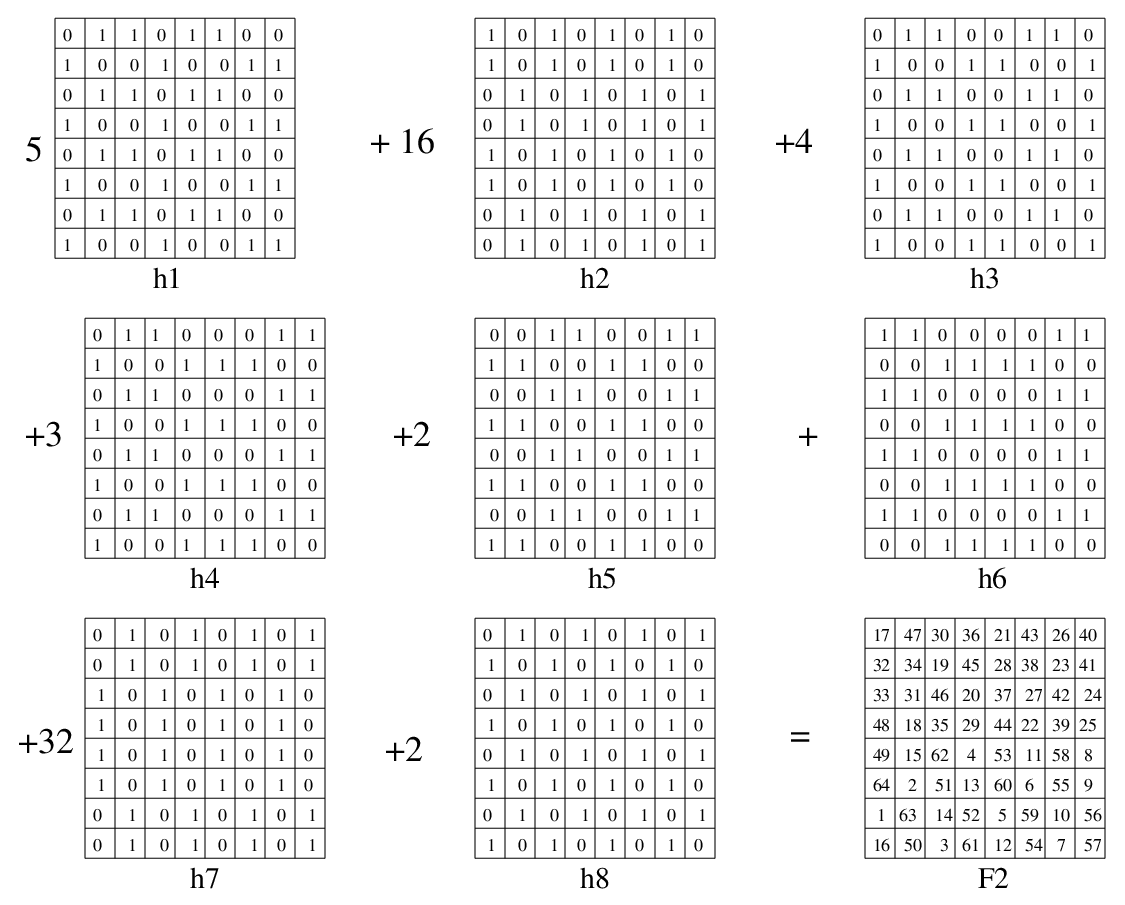
Similarly, let

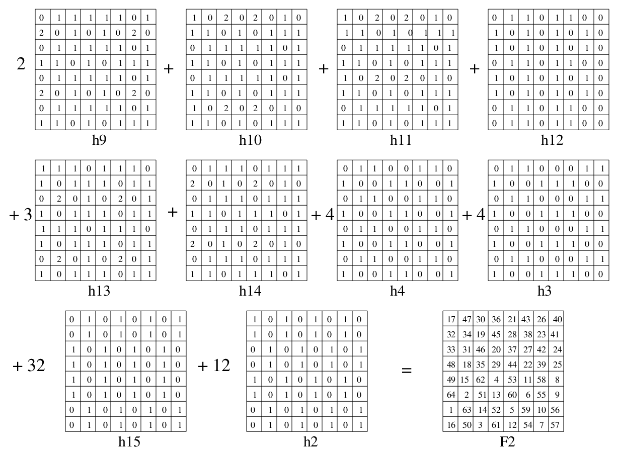
\begin{array}[]{l}\mbox{g}1=(r_{3},r_{5})\cdot(r_{4},r_{6})\cdot(r_{11},r_{13})\cdot(r_{12},r_{14})\cdot\mbox{S2},\hskip 3.61371pt\mbox{g}2=\mbox{S1},\hskip 3.61371pt\mbox{g}3=R\cdot\mbox{g}1,\\ \mbox{g}4=(r_{1},r_{5})\cdot(r_{4},r_{8})\cdot(r_{9},r_{13})\cdot(r_{12},r_{16})\cdot\mbox{S2},\hskip 3.61371pt\mbox{g}5=\mbox{ transpose of }S2,\\ \mbox{g}6=(c_{9},c_{13})\cdot(c_{10},c_{14})\cdot(c_{11},c_{15})\cdot(c_{12},c_{16})\cdot\mbox{g}5,\\ \mbox{g}7=(r_{2},r_{6})\cdot(r_{10},r_{14})\cdot(r_{12},r_{16})\cdot\mbox{S2},\\ \mbox{g}8=\mbox{S3},\hskip 3.61371pt\mbox{g}9=(r_{1},r_{5})\cdot(r_{3},r_{7})\cdot(r_{10},r_{14})\cdot(r_{12},r_{16})\cdot\mbox{S2},\\ \mbox{g}10=(r_{2},r_{6})\cdot(r_{4},r_{8})\cdot(r_{10},r_{14})\cdot(r_{12},r_{16})\cdot\mbox{S2},\\ \mbox{g}11=(r_{2},r_{6})\cdot(r_{3},r_{7})\cdot(r_{9},r_{13})\cdot(r_{10},r_{14})\cdot(r_{12},r_{16})\cdot\mbox{S2}.\end{array}

These constructions, as we saw before in Section 1.2 are not unique. A different construction of F2 is given in Figure 3.3.

Interestingly, the Hilbert basis of $8\times 8$ pandiagonal Franklin squares is a subset of the Hilbert basis of $8\times 8$ Franklin squares. The thirty-two squares generated by the action of the group $G$ on T2 and $R\cdot$ T2 form the Hilbert basis of $8\times 8$ pandiagonal Franklin squares. The pandiagonal Franklin squares in Figure 3.4 were constructed by Ray Hagstorm using the minimal Hilbert basis of Pandiagonal Franklin squares [36].

Let $F_{8}(s)$ denote the number of $8\times 8$ Franklin squares with magic sum $s$ . We used the program CoCoA to compute the Hilbert-Poincaré series $\sum_{s=0}^{\infty}F_{8}(s)t^{s}$ and obtained

\begin{array}[]{l}\sum_{s=0}^{\infty}F_{8}(s)t^{s}=\\ \\ \{({t}^{36}-{t}^{34}+28\,{t}^{32}+33\,{t}^{30}+233\,{t}^{28}+390\,{t}^{26}+947\,{t}^{24}+1327\,{t}^{22}+1991\,{t}^{20}\\ +1878\,{t}^{18}+1991\,{t}^{16}+1327\,{t}^{14}+947\,{t}^{12}+390\,{t}^{10}+233\,{t}^{8}+33\,{t}^{6}+28\,{t}^{4}\\ -{t}^{2}+1)\}/\{({t}^{2}-1)^{7}({t}^{6}-1)^{3}({t}^{2}+1)^{6}\}\\ \\ =1+34\,{t}^{4}+64\,{t}^{6}+483\,{t}^{8}+1152\,{t}^{10}+4228\,{t}^{12}+9792\,{t}^{14}+25957\,{t}^{16}+\cdots\end{array}

We recover the Hilbert function $F_{8}(s)$ from the Hilbert-Poincaré series by interpolation (see Section 1.2). The formulas for the number of $8\times 8$ pandiagonal Franklin squares in Theorem 1.4.4 are derived similarly.

Natural $8\times 8$ Franklin squares always have magic sum 260. From Theorem 1.4.3 we find that $F_{8}(260)$ is 228,881,701,845,346. This number is an upper bound for the number of natural $8\times 8$ Franklin squares. The actual number of such squares is still an open question.

3.2 A few aspects of $16\times 16$ Franklin squares.

Finding the minimal Hilbert basis for the cone of $16\times 16$ Franklin squares is computationally challenging and remains an unresolved problem. However, we can provide a partial Hilbert basis that enables us to construct Benjamin Franklin’s square F3, as well as the square N4. The following lemma proves that every $8\times 8$ Franklin square corresponds to a $16\times 16$ Franklin square.

Lemma 3.2.1.

Let M be an $8\times 8$ Franklin square. Then the square T constructed using M as blocks (as in Figure 3.5) is a $16\times 16$ Franklin square.

Proof. Let the magic sum of M be $s$ . The half-columns and half-rows of T add up to $s$ since they are the columns and rows of M, respectively. Also the columns and rows of T add to $2s$ . The bent diagonals of T sum to $2s$ (see Figure 3.6 for an explanation). Since the $2\times 2$ subsquares of M add to $s/2$ , we infer that the $2\times 2$ subsquares of T add to $s/2$ . Thus T is a $16\times 16$ Franklin square with magic sum $2s$ . $\square$

Consider the set $\cal{B}$ of $16\times 16$ Franklin squares obtained by applying the symmetry operations listed in Theorem 1.4.1 to the squares constructed by applying Lemma 3.2.1 to the ninety-eight elements of the minimal Hilbert basis of $8\times 8$ Franklin squares (for example, S1 in Figure 3.7 is constructed from the $8\times 8$ Franklin square T1 in Figure 3.1) and the $16\times 16$ Franklin squares S2 and S3 in Figure 3.7. Observe that one-fourth the magic sum of a $16\times 16$ Franklin square is always an integer because its $2\times 2$ subsquares add to this number. This implies that the squares in $\cal{B}$ are irreducible, for they have magic sums 8 or 12 (it is easy to verify that there are no $16\times 16$ Franklin squares of magic sum 4). Therefore, $\cal{B}$ is a subset of the minimal Hilbert basis for the cone of $16\times 16$ Franklin squares. Thus, $\cal B$ forms a partial Hilbert basis.

We obtain F3 and N4 as follows:

\begin{array}[]{lll}\mbox{F3}&=&\mbox{g}1+17\cdot\mbox{g}2+32\cdot\mbox{g}3+\mbox{g}4+64\cdot\mbox{g}5+128\cdot\mbox{g}6+2\cdot\mbox{g}7+2\cdot\mbox{g}8+7\cdot\mbox{g}9\\ &&+\mbox{g}10+2\cdot\mbox{g}11;\\ \\ \mbox{N4}&=&\mbox{g}1+17\cdot\mbox{g}2+64\cdot\mbox{g}3+\mbox{g}4+32\cdot\mbox{g}5+128\cdot\mbox{g}6+2\cdot\mbox{g}7+2\cdot\mbox{g}8+7\cdot\mbox{g}9\\ &&+\mbox{g}10+2\cdot\mbox{g}11.\par\end{array}

Since every $8\times 8$ Franklin square corresponds to a $16\times 16$ Franklin square by Lemma 3.2.1, the formulas for the number of $8\times 8$ Franklin squares of magic sum $s$ in Theorem 1.4.3 also yields a lower bound for the number of $16\times 16$ Franklin squares of magic sum $2s$ .

3.3 Symmetries of Franklin Squares.

In this section we prove Theorem 1.4.2, which asserts that the new Franklin squares N1, N2, N3, and N4 are not derived from Benjamin Franklin’s squares F1, F2, or F3 by symmetry operations. We first prove Theorem 1.4.1.

Rotation, reflection, and taking the transpose are plainly symmetry operations on Franklin squares. The proof of Theorem 1.4.1 follows from Lemmas 3.3.1, 3.3.2, 3.3.3, and 3.3.4.

Let $S_{n}$ denote the group of $n\times n$ permutation matrices acting on $n\times n$ matrices. As earlier, let $(r_{i},r_{j})$ denote the operation of exchanging rows $i$ and $j$ of a square matrix, and let $(c_{i},c_{j})$ denote the analogous operation on columns.

Lemma 3.3.1.

Let $G$ be the subgroup of $S_{8}$ generated by

\{(c_{1},c_{3}),(c_{5},c_{7}),(c_{2},c_{4}),(c_{6},c_{8}),(r_{1},r_{3}),(r_{5},r_{7}),(r_{2},r_{4}),(r_{6},r_{8})\},

and let $H$ be the subgroup of $S_{16}$ generated by

\begin{array}[]{l}\{(c_{1},c_{3}),(c_{2},c_{4}),(c_{3},c_{5}),(c_{4},c_{6}),(c_{5},c_{7})(c_{6},c_{8}),(c_{9},c_{11}),(c_{10},c_{12}),\\ (c_{11},c_{13}),(c_{12},c_{14}),(c_{13},c_{15})(c_{14},c_{16}),(r_{1},r_{3}),(r_{2},r_{4}),(r_{3},r_{5}),(r_{4},r_{6}),\\ (r_{5},r_{7})(r_{6},r_{8}),(r_{9},r_{11}),(r_{10},r_{12}),(r_{11},r_{13}),(r_{12},r_{14}),(r_{13},r_{15}),(r_{14},r_{16})\}.\end{array}

The row and column permutations from the group $G$ map $8\times 8$ Franklin squares to $8\times 8$ Franklin squares, while the row and column permutations from the group $H$ map $16\times 16$ Franklin squares to $16\times 16$ Franklin squares.

Proof. Clearly exchanging rows or columns of a Franklin square preserves row and column sums. Half-row and half-column sums are preserved because the permutations of rows and columns included here operate in some half of a Franklin square. That $2\times 2$ subsquare sums are preserved follows from the fact that every alternate pair of entries in a pair of columns or rows add to the same sum (see Figure 3.8 for an explanation). For any $3\times 3$ subsquare of a Franklin square, the two sums of diagonally opposite elements are equal (see Figure 3.8 for details). This implies that, if we permute alternate rows or alternate columns then the new entries preserve bent diagonal sums. Observe that for the preservation of bent diagonal sums, it is critical that the alternate row and column permutations be restricted to act in one half of a Franklin square (see Figure 1.21 for examples). $\square$

Lemma 3.3.2.

Let $S$ be the subgroup of $S_{16}$ generated by the set

\begin{array}[]{l}\{(r_{1},r_{5}),(r_{2},r_{6}),(r_{3},r_{7}),(r_{4},r_{8}),(r_{9},r_{13}),(r_{10},r_{14}),(r_{11},r_{15}),(r_{12},r_{16}),\\ (c_{1},c_{5}),(c_{2},c_{6}),(c_{3},c_{7}),(c_{4},c_{8}),(c_{9},c_{13}),(c_{10},c_{14}),(c_{11},c_{15}),(c_{12},c_{16})\}.\end{array}

The row and column permutations from the subgroup $S$ map $16\times 16$ Franklin squares to $16\times 16$ Franklin squares.

Proof. Half-column and half-row sums are preserved because the specified row or column exchanges only affect some half of the $16\times 16$ Franklin square. Because of the $2\times 2$ subsquare sum property, we see that every $4\times 4$ subsquare adds to the common magic sum. Hence the two sums of diagonally opposite elements in a $5\times 5$ subsquare are equal (see Figure 3.9 for an explanation). This implies that the bent diagonal sums are preserved, again because they operate in only one-half of a Franklin square. It is easy to verify that all other sums are preserved under the action of elements of $S$ . $\square$

Observe that the groups $G$ , $H$ , and $S$ are commutative, for each nonidentity element in each of these groups has order 2. Therefore the order of $G$ is $2^{8}$ , the order of $H$ is $2^{24}$ , and the order of $S$ is $2^{16}$ .

Lemma 3.3.3.

The operation of interchanging the first $n/2$ columns (respectively, rows) and the last $n/2$ columns (respectively, rows) of an $n\times n$ Franklin square is a symmetry operation.

Proof. These operations preserve half-row and half-column sums. The row sums and column sums do not change. Bent diagonal and $2\times 2$ subsquare sums are preserved because of continuity (see Figure 3.10 for examples). $\square$

Lemma 3.3.4.

Simultaneously interchanging all the adjacent columns (respectively, rows) $i$ and $i+1$ ( $i=1,3,5,\dots,n-1$ ) of an $n\times n$ Franklin square is a symmetry operation.

Proof. It is clear that row, column, half-row, and half-column sums are preserved by these operations. Moreover $2\times 2$ subsquare sums are preserved because every alternate pair of entries in a pair of columns or rows add to the same sum (see Figure 3.8). Bent diagonal sums are preserved because of the $2\times 2$ subsquare sum property. See Figure 3.11 for an explanation (the explanation for bent diagonal sums of $16\times 16$ Franklin squares is similar). $\square$

Are the symmetry operations given in Theorem 1.4.1 all the symmetry operations of a Franklin square? We do not know the answer to this question, but the symmetries described in this section enable us to interchange any two rows or any two columns within any half of a Franklin square and get a Franklin square. Note that certain row or column exchanges are not symmetry operations unless they are accompanied by other simultaneous row or column exchanges. We now show that N1, N2, N3, and N4 are not symmetric transformations of F1, F2, or F3.

Lemma 3.3.5.

The squares F1 and F2 can be transformed by means of symmetry operations neither to each other nor to any of the nonisomorphic squares N1, N2, or N3.

Proof. By definition, symmetry operations map a Franklin square to another Franklin square. We can permute the entries of the Franklin square F2 to get F1, N1, N2, and N3 (see Figure 3.12). The permutation that maps F2 to N2 is not, however, a symmetry operation: F1 does not transform to a Franklin square under this permutation since bent diagonal sums are not preserved. The other permutations of F2 in Figure 3.12 likewise fail to be symmetries. Again, F1 does not map to a Franklin square under these permutations for half-column sums are not preserved. Thus F2 cannot be transformed to F1, N1, N2, or N3 using symmetry operations. Similarly, the permutations of the entries of F1 that map it to F2, N1, N2, and N3, respectively, are not symmetry operations because F2 is not mapped to a Franklin square under any of these permutations (in these instances half-row sums are not preserved). The permutations that map the square N1 to N2 and N3, and the permutations that map N2 to N1 and N3 are not symmetry operations because F1 is not mapped to a Franklin square under these permutations (half-column sums of F1 are not preserved for all these permutations). Similarly, the permutations that map N3 to N1 and N2 are not symmetry operations because F2 is not mapped to a Franklin square under these operations. Therefore, the squares N1, N2, and N3 are not isomorphic to each other. $\square$

Lemma 3.3.6.

The square F3 cannot be transformed to N4 using symmetry operations.

Proof. Permuting the entries of F3 to get N4 is achieved by simultaneously interchanging columns 1 and 15, columns 2 and 16, columns 7 and 9, and columns 8 and 10 of F3. This permutation is not a symmetry operation. To see this, note that the square A obtained by transposing F3 is a Franklin square (Theorem 1.4.1). But $(c_{1},c_{15})(c_{2},c_{16})(c_{7},c_{9})(c_{8},c_{10})\cdot$ A is not a Franklin square, since bent diagonal sums are not preserved. $\square$

Lemmas 3.3.5 and 3.3.6, in tandem, establish Theorem 1.4.2.

Chapter 4 Symmetric Magic Squares and the Magic Graphs Connection

What immortal hand or eye
Dare frame thy fearful symmetry?

– William Blake.

4.1 Hilbert bases of polyhedral cones of magic labelings.

In this section we derive some results about Hilbert bases of cones of magic labelings of graphs and also prove Proposition 1.5.3.

Lemma 4.1.1.

Let $G$ be a graph with $n$ vertices. A labeling $L$ of $G$ with magic sum $s$ can be lifted to a magic labeling $L^{\prime}$ of $\Gamma_{n}$ with magic sum $s$ .

Proof. Since $G$ is a subgraph of $\Gamma_{n}$ , every labeling $L$ of $G$ can be lifted to a labeling $L^{\prime}$ of $\Gamma_{n}$ , where

L^{\prime}(e_{ij})=\left\{\begin{array}[]{ll}L(e_{ij})&\mbox{ if $e_{ij}$ is also an edge of $G$,}\\ 0&\mbox{otherwise.}\end{array}\right.

Since the edges with nonzero labels are the same for both $L$ and $L^{\prime}$ , it follows that the magic sums are also the same. $\square$

Lemma 4.1.2.

Let $G$ be a graph with $n$ vertices. The minimal Hilbert basis of $C_{G}$ can be lifted to a subset of the minimal Hilbert basis of $C_{\Gamma_{n}}$ .

Proof. If $L$ is an irreducible magic labeling of $G$ , then clearly it lifts to an irreducible magic labeling $L^{\prime}$ of $\Gamma_{n}$ . Since the minimal Hilbert basis is the set of all irreducible magic labelings, we get that the minimal Hilbert basis of $C_{G}$ corresponds to a subset of the minimal Hilbert basis of $C_{\Gamma_{n}}$ . $\square$

For example, the magic labelings O1 and O2 of the octahedral graph in Figure 4.4 correspond to the magic labelings a1 and a2, respectively, of $\Gamma_{6}$ (see Figure 4.11).

Similarly, we can prove:

Lemma 4.1.3.

For a digraph $D$ with $n$ vertices, a magic labeling $L$ with magic sum $s$ can be lifted to a magic labeling $L^{\prime}$ of $\Pi_{n}$ with the same magic sum $s$ . The minimal Hilbert basis of $C_{D}$ can be lifted to a subset of the minimal Hilbert basis of $C_{\Pi_{n}}$ .

Lemma 4.1.4.

Let $D$ be a digraph with $n$ vertices. All the elements of the minimal Hilbert basis of $C_{D}$ have magic sum 1.

Proof. It is well-known that the minimal Hilbert basis of semi-magic squares are the permutation matrices (see [51]) and therefore have magic sum 1. The one-to-one correspondence between magic labelings of $\Pi_{n}$ and semi-magic squares implies that the minimal Hilbert basis elements of $C_{\Pi_{n}}$ have magic sum 1. It follows by Lemma 4.1.3 that all the elements of the minimal Hilbert basis of $C_{D}$ have magic sum 1. $\square$

We now present the proof of the fact that perfect matchings of bipartite graphs correspond to the elements of the minimal Hilbert basis of its corresponding digraph.

Proof of Proposition 1.5.3.

Every element of the minimal Hilbert basis of $C_{B_{D}}$ corresponds to a perfect matching of $B$ by Lemma 4.1.4. Moreover, all the magic labelings of $B_{D}$ of magic sum 1 belong to the minimal Hilbert basis of $C_{B_{D}}$ because they are irreducible. Since perfect matchings of $B$ are in one-to-one correspondence with magic labelings of $B_{D}$ of magic sum 1, we derive that perfect matchings of $B$ are in one-to-one correspondence with the elements of the minimal Hilbert basis of $C_{B_{D}}$ . It follows that $H_{B_{D}}(1)$ is the number of perfect matchings of $B$ . $\square$

For example, consider the Octahedral graph with the given orientation $D_{O}$ in Figure 1.27. The minimal Hilbert basis of $D_{O}$ is given in Figure 4.1. The perfect matchings of the bipartite graph $G_{D_{O}}$ corresponding to the minimal Hilbert basis elements of $C_{D_{O}}$ is given in Figure 4.2. We derive $H_{D_{O}}(r)=r+1$ and thereby verify that the number of perfect matchings of $G_{D_{O}}$ is indeed 2.

4.2 Counting isomorphic simple labelings and Invariant rings.

Let $S_{n}$ denote the group of permutations that acts on the vertex set $\{v_{1},v_{2},\dots,v_{n}\}$ of $G$ . Let $e_{ij}$ denote an edge between the vertices $v_{i}$ and $v_{j}$ . The action of $S_{n}$ on the vertices of $G$ translates to an action on the labels of the edges of $G$ by

\sigma(L(e_{ij}))=L(e_{\sigma(i)\sigma(j)})\mbox{ where }\sigma\in S_{n}.

Two labelings $L$ and $L^{\prime}$ of $G$ are isomorphic if there exists a permutation $\sigma$ in $S_{n}$ such that $L^{\prime}(e_{ij})=L(e_{\sigma(i)\sigma(j)})$ , i.e. $\sigma(L)=L^{\prime}$ . A set $S=\{g_{1},g_{2},\dots,g_{r}\}$ is said to generate the minimal Hilbert basis of the cone of magic labelings of $G$ if every element of the minimal Hilbert basis is isomorphic to some $g_{i}$ in $S$ . For example, T1 generates the minimal Hilbert basis of the cone of magic labelings of the tetrahedral graph (see Figure 4.3). Observe that we get T2 by permuting the vertices $v_{2}$ and $v_{4}$ of T1, and T3 by permuting the vertices $v_{3}$ and $v_{4}$ of T1.

Proposition 4.2.1.

Let $L$ be a magic labeling in the minimal Hilbert basis of the cone of magic labelings of a graph (or a digraph), then all the labelings isomorphic to $L$ also belong to the minimal Hilbert basis.

Proof. Let $L^{\prime}$ be a labeling isomorphic to $L$ and $\sigma$ in $S_{n}$ be such that $\sigma(L)=L^{\prime}$ . Suppose $L^{\prime}$ does not belong to the Hilbert basis. Then $L^{\prime}$ is reducible and can be written as sum of two labelings: $L^{\prime}=L_{1}+L_{2}$ . But, ${\sigma}^{-1}(L^{\prime})=L$ . Therefore, ${\sigma}^{-1}(L_{1})+{\sigma}^{-1}(L_{2})=L$ . This is not possible because $L$ is irreducible, since it belongs to the minimal Hilbert basis. Therefore, we conclude that $L^{\prime}$ must also belong to the Hilbert basis. $\square$

A labeling of $G$ is called a simple labeling if the labels are 0 or 1. Invariant theory [59] provides an efficient algebraic method of counting isomorphic simple labelings of a graph $G$ . Let $L$ be a simple labeling of $G$ . Let $X^{L}$ denote the monomial

X^{L}=\prod_{i,j=1,\dots,n}x_{ij}^{L({e_{ij}})}.

Consider the polynomial

{\left(X^{L}\right)}^{\circledast}=\sum_{\sigma\in S_{n}}X^{\sigma(L)},\hskip 7.22743pt\mbox{ where }X^{\sigma(L)}=\prod_{i,j=1,\dots,n}x_{ij}^{L(e_{\sigma(i)\sigma(j)})}.

Observe that ${\left(X^{L}\right)}^{\circledast}$ is an invariant polynomial under the action of $S_{n}$ on the indices of the variables $x_{ij}$ . Let $k$ be any field. The set of polynomials invariant in the polynomial ring $k[x_{ij}]$ under the action of the group $S_{n}$ is called the invariant ring of $S_{n}$ and is denoted by $k[x_{ij}]^{S_{n}}$ . See [59] for an introduction to invariant rings.

Consider the simple labeling $L_{G}$ of $\Gamma_{n}$ associated to $G$ :

L_{G}(e_{ij})=\left\{\begin{array}[]{ll}1&\mbox{if $e_{ij}$ is an edge of $G$,}\\ 0&\mbox{otherwise.}\end{array}\right.

Then the polynomial ${\left(X^{L}\right)}^{\circledast}$ evaluated at $L_{G}$ counts the number of labelings of $G$ that are isomorphic to $L$ .

For example, consider the Octahedral graph ${\cal O}$ with the labeling O1 in Figure 4.4. Then,

\begin{array}[]{ll}{\left(X^{O1}\right)}^{\circledast}=&x_{14}x_{23}x_{56}+x_{16}x_{23}x_{45}+x_{13}x_{26}x_{45}+x_{12}x_{36}x_{45}+x_{15}x_{23}x_{46}+x_{13}x_{25}x_{46}+\\ &x_{16}x_{25}x_{34}+x_{15}x_{26}x_{34}+x_{12}x_{34}x_{56}+x_{12}x_{35}x_{46}+x_{13}x_{24}x_{56}+x_{16}x_{24}x_{35}+\\ &x_{14}x_{26}x_{35}+x_{15}x_{24}x_{36}+x_{14}x_{25}x_{36}.\end{array}

Substituting $x_{12}=x_{13}=x_{14}=x_{15}=x_{23}=x_{24}=x_{26}=x_{35}=x_{36}=x_{x45}=x_{46}=x_{56}=1$ and $x_{11}=x_{22}=x_{33}=x_{44}=x_{55}=x_{66}=x_{16}=x_{25}=x_{34}=0$ in ${\left(X^{O1}\right)}^{\circledast}$ , we get that

{\left(X^{O1}\right)}^{\circledast}(L_{\cal O})=8.

Therefore, there are 8 magic labelings in the $S_{6}$ orbit of the magic labeling O1 of the octahedral graph. Similarly, there are four magic labelings in the orbit of O2. The generators of the Hilbert basis of the Octahedral graph are given in Figure 4.4. The numbers in square brackets in the figures indicate the number of elements in the orbit class of each generator throughout the article.

For digraphs, we assign a variable $x_{ij}$ to every directed edge $e_{ij}$ , and use the corresponding invariant ring to count isomorphic simple labelings. See [61] for more aspects of labeled graph isomorphisms and invariant rings.

Since all the elements of the minimal Hilbert basis of $C_{D}$ , where $D$ is a digraph, are simple labelings, we can use invariant theory effectively. Since the number of elements in the minimal Hilbert basis of semi-magic squares (and hence $C_{\Pi_{n}}$ ) is $n!$ (see [51]), we can list all the generators of the minimal Hilbert basis of $C_{\Pi_{n}}$ . The generators of the Hilbert basis of $C_{\Pi_{6}}$ are given in Figure 4.5.

Algorithm 4.2.1.

Computing minimal Hilbert basis of a finite digraph $D$ with $n$ vertices.

Input: A digraph $D$ with $n$ vertices and the set of $n\times n$ permutation matrices.

Output: The minimal Hilbert basis of the finite digraph $D$ .

Step 0. List a set of generators of the minimal Hilbert basis of $C_{\Pi_{n}}$ .

Step 1. Choose all the elements $h_{i}$ among the generators of the minimal Hilbert basis of $C_{\Pi_{n}}$ which have the edges not in $D$ labeled 0. Delete the edges in $h_{i}$ that are not in $D$ to get a magic labeling $g_{i}$ of $D$ .

Step 2. $g_{i}$ and the magic labelings isomorphic to $g_{i}$ form the minimal Hilbert basis of the cone of magic labelings of $D$ .

For example, consider the digraph $D$ that have all the edges of $\Pi_{6}$ except the loops. Then the minimal Hilbert basis of $D$ are the 265 labelings corresponding to the labelings s1, s2, s7, and s11 in Figure 4.5 and their isomorphic magic labelings.

4.3 Polytopes of magic labelings.

The proofs of Theorems 1.5.4, 1.5.5, and 1.5.6, and Corollary 1.5.4.1 are presented in this section.

Let $G$ be a positive graph. An element $\beta$ in the semigroup $S_{C_{G}}$ is said to be completely fundamental, if for any positive integer $n$ and $\alpha,{\alpha}^{\prime}\in S_{C_{G}}$ , $n\beta=\alpha+{\alpha}^{\prime}$ implies $\alpha=i\beta$ and ${\alpha}^{\prime}=(n-i)\beta$ , for some positive integer $i$ , such that $0\leq i\leq n$ (see [54]).

Lemma 4.3.1.

${\cal P}_{G}$ is a rational polytope.

Proof. Proposition $4.6.10$ of Chapter 4 in [54] states that the set of extreme rays of a cone and the set of completely fundamental solutions are identical. Proposition 2.7 in [55] states that every completely fundamental magic labeling of a graph $G$ has magic sum 1 or 2. Thus, the extreme rays of the cone of magic labelings of a graph $G$ are irreducible 2-matchings of $G$ . We get a vertex of ${\cal P}_{G}$ by dividing the entries of a extreme ray by its magic sum. Thus, ${\cal P}_{G}$ is a rational polytope. $\square$

Lemma 4.3.2.

The dimension of ${\cal P}_{G}$ is $q-n+b$ , where $q$ is the number of edges of $G$ , $n$ is the number of vertices, and $b$ is the number of connected components that are bipartite.

Proof. Ehrhart’s theorem states that the degree of $H_{G}(r)$ is the dimension of ${\cal P}_{G}$ [12]. The degree of $H_{G}(r)$ is $q-n+b$ by Theorem 1.5.2. Therefore, the dimension of ${\cal P}_{G}$ is $q-n+b$ . $\square$

Lemma 4.3.3.

The $d$ -dimensional faces of ${\cal P}_{G}$ are the $d$ -dimensional polytopes of magic labelings of positive subgraphs of $G$ with $n$ vertices and at most $n-b+d$ edges.

Proof. An edge $e$ labeled with a zero in a magic labeling $L$ of $G$ does not contribute to the magic sum, therefore, we can consider $L$ as a magic labeling of a subgraph of $G$ with the edge $e$ deleted. Since a face of ${\cal P}_{G}$ is the set of magic labelings of $G$ where some edges are always labeled zero, it follows that the face is also the set of all the magic labelings of a subgraph of $G$ with these edges deleted. Similarly, every magic labeling of a subgraph $H$ with $n$ vertices corresponds to a magic labeling of $G$ , where the missing edges of $G$ in $H$ are labeled with 0. Now, let $H$ be a subgraph such that the edges $e_{r1},\dots,e_{rm}$ are labeled zero for every magic labeling of $H$ . Then the face defined by $H$ is same as the face defined by the positive graph we get from $H$ after deleting the edges $e_{r1},\dots,e_{rm}$ . Therefore, the faces of ${\cal P}_{G}$ are polytopes of magic labelings of positive subgraphs.

By Lemma 4.3.2, the dimension of ${\cal P}_{G}$ is $q-n+b$ . Therefore, to get a $d$ -dimensional polytope, we need to label at least $q-n+b-d$ of $G$ edges always 0. This implies that the $d$ -dimensional face is the set of magic labelings of a positive subgraph of $G$ with $n$ vertices and at most $n-b+d$ edges. $\square$

The proof of Theorem 1.5.4 follows from Lemmas 4.3.1, 4.3.2, and 4.3.3. We can now prove Corollary 1.5.4.1.

Proof of Corollary 1.5.4.1.

It is clear from the one-to-one correspondence between magic labelings of $\Gamma_{n}$ and symmetric magic squares that ${\cal P}_{\Gamma_{n}}$ has the following description:

\begin{array}[]{lll}{\cal P}_{\Gamma_{n}}&=&\{L=(L(e_{ij})\in{\mathbb{R}}^{\frac{n(n+1)}{2}};L(e_{ij})\geq 0;1\leq i,j\leq n,i\leq j,\\ &&\sum_{j=1}^{i}L(e_{ji})+\sum_{j=i+1}^{n}L(e_{ij})=1\mbox{ for }i=1,\dots,n\}.\end{array}

Since the graph ${\Gamma_{n}}$ has $\frac{n(n+1)}{2}$ edges and $n$ vertices, and every graph is a subgraph of $\Gamma_{n}$ , it follows from Theorem 1.5.4 that the dimension of ${\cal P}_{\Gamma_{n}}$ is $\frac{n(n-1)}{2}$ ; the $d$ -dimensional faces of ${\cal P}_{\Gamma_{n}}$ are $d$ -dimensional polytopes of magic labelings of positive graphs with $n$ vertices and at most $n+d$ edges.

We can partition the vertices of $\Gamma_{2n}$ into two equal sets $A$ and $B$ in ${2n-1}\choose n$ ways: Fix the vertex $v_{1}$ to be in the set $A$ , then we can choose the n vertices for the set $B$ in ${2n-1}\choose n$ ways, and the remaining $n-1$ vertices will belong to the set $A$ . By adding the required edges, we get a complete bipartite graph for every such partition of the vertices of $\Gamma_{2n}$ . Thus, the number of subgraphs of $\Gamma_{2n}$ that are isomorphic to $K_{n,n}$ is ${2n-1}\choose n$ . Therefore, there are $2n-1\choose n$ faces of ${\cal P}_{\Gamma_{2n}}$ that are Birkhoff polytopes because every isomorphic copy of $K_{n,n}$ contributes to a face of ${\cal P}_{\Gamma_{2n}}$ . $\square$

We now prove our results about polytopes of magic digraphs.

Proof of Theorem 1.5.5. By Lemma 4.1.4, all the elements of the Hilbert basis of $C_{D}$ have magic sum 1. Since the extreme rays are a subset of the Hilbert basis elements, it follows that the vertices of ${\cal P}_{D}$ are integral. Since ${\cal P}_{D}={\cal P}_{G_{D}}$ , it follows by Theorem 1.5.4 that the dimension of ${\cal P}_{D}$ is $q-2n+b$ ; the $d$ -dimensional faces of ${\cal P}_{D}$ are the $d$ -dimensional polytopes of magic labelings of positive subdigraphs of $D$ with $n$ vertices and at most $2n-b+d$ edges. $\square$

We derive our results about the faces of the Birkhoff polytope as a consequence.

Proof of Theorem 1.5.6. The one-to-one correspondence between semi-magic squares and magic labelings of ${\Pi_{n}}$ gives us that ${\cal P}_{\Pi_{n}}=B_{n}$ . Since every digraph with $n$ vertices is a subdigraph of $\Pi_{n}$ , by Theorem 1.5.5, it follows that its $d$ -dimensional faces are $d$ -dimensional polytopes of magic labelings of positive digraphs with $n$ vertices and at most $2n-1+d$ edges. Since the vertex set of a face of $B_{n}$ is a subset of the vertex set of $B_{n}$ it follows that the vertices of ${\cal P}_{D}$ , where $D$ is a positive digraph, are permutation matrices. $\square$

Our results enable us to reprove some known facts about the Birkhoff polytope as well. For example, Theorem 1.5.5 gives us that the dimension of $B_{n}$ is ${(n-1)}^{2}$ . The leading coefficient of the Ehrhart polynomial of $B_{n}$ is the volume of $B_{n}$ . This number has been computed for $n=1,2,\dots,9$ (see [11] and [23]).

4.4 Computational results

We will now list our computational results. The numbers in square brackets in the figures represent the number of elements in the orbit class of each generator.

4.4.1 Symmetric magic squares.

The generators of the minimal Hilbert basis of $C_{\Gamma_{n}}$ for $n=1,2,3,4,5$ , and $6$ are given in Figures 4.6, 4.7, 4.8, 4.9, 4.10, and 4.11, respectively. It is interesting that all the elements of the minimal Hilbert basis of $C_{\Gamma_{n}}$ for $n=1,\dots,6$ are 2-matchings. The minimal Hilbert basis elements are not, in general, 2-matchings for all $n$ (see Figure 4.12 for examples of irreducible magic labelings of magic sum 3). In fact, it follows from the results of chapter 11 in [41], that there exists a graph with an irreducible magic labeling of magic sum $r$ if and only if $r$ is 2 or $r$ is odd. By Proposition 4.1.2, this implies, that there is a minimal Hilbert basis element of magic sum $r$ of $C_{\Gamma_{n}}$ , for some $n$ , if and only if, $r$ is 2 or $r$ is odd. The program 4ti2 was also able to compute the minimal Hilbert bases of $C_{\Gamma_{7}}$ and $C_{\Gamma_{8}}$ .

Recall that the number of $n\times n$ symmetric magic squares is the same as $H_{\Gamma_{n}}(r)$ (the generating functions for $H_{\Gamma_{n}}(r)$ for $n$ up to 5 are given in [56]). The volume of ${\cal P}_{\Gamma_{n}}$ is the leading coefficient of $H_{\Gamma_{n}}(r)$ .

H_{\Gamma_{1}}(r)=1\mbox{ for all $r\geq 0$.}

H_{\Gamma_{2}}(r)=r+1\mbox{ for all $r\geq 0$.}

H_{\Gamma_{3}}(r)=\left\{\begin{array}[]{ll}\frac{1}{4}r^{3}+\frac{9}{8}r^{2}+\frac{7}{4}r+1&\mbox{if 2 divides $r$,}\\ \\ \frac{1}{4}r^{3}+\frac{9}{8}r^{2}+\frac{7}{4}r+\frac{7}{8}&\mbox{ otherwise.}\end{array}\right.

H_{\Gamma_{4}}(r)=\left\{\begin{array}[]{ll}{\frac{1}{72}}{r}^{6}+\frac{1}{6}{r}^{5}+{\frac{119}{144}}{r}^{4}+{\frac{13}{6}}{r}^{3}+{\frac{29}{9}}{r}^{2}+\frac{8}{3}r+1&\mbox{if 2 divides $r$,}\\ \\ {\frac{1}{72}}{r}^{6}+\frac{1}{6}{r}^{5}+{\frac{119}{144}}{r}^{4}+{\frac{13}{6}}{r}^{3}+{\frac{29}{9}}{r}^{2}+\frac{8}{3}r+{\frac{15}{16}}&\mbox{ otherwise.}\end{array}\right.

H_{\Gamma_{5}}(r)=\left\{\begin{array}[]{l}{\frac{365}{3096576}}{r}^{10}+{\frac{9125}{3096576}}{r}^{9}+{\frac{22553}{688128}}{r}^{8}+{\frac{55085}{258048}}{r}^{7}+{\frac{11083}{12288}}{r}^{6}+{\frac{7945}{3072}}{r}^{5}+{\frac{1978913}{387072}}{r}^{4}\\ \\ +{\frac{335065}{48384}}{r}^{3}+{\frac{50329}{8064}}{r}^{2}+{\frac{1177}{336}}r+1\\ \hfill\mbox{if 2 divides $r$,}\\ \\ \\ {\frac{365}{3096576}}{r}^{10}+{\frac{9125}{3096576}}{r}^{9}+{\frac{22553}{688128}}{r}^{8}+{\frac{55085}{258048}}{r}^{7}+{\frac{11083}{12288}}{r}^{6}+{\frac{63545}{24576}}{r}^{5}+{\frac{15807679}{3096576}}{r}^{4}\\ \\ +{\frac{5329855}{774144}}{r}^{3}+{\frac{6327137}{1032192}}{r}^{2}+{\frac{1139917}{344064}}r+{\frac{27213}{32768}}\\ \hfill\mbox{ otherwise.}\end{array}\right.

4.4.2 Pandiagonal symmetric magic squares.

Pandiagonal symmetric magic squares are symmetric magic squares such that all the pandiagonals also add to the magic sum (see Figure 1.4). The generators of the Hilbert basis of $n\times n$ pandiagonal symmetric magic squares for $n=3$ , $4$ , and $5$ are given in Figures 4.13, 4.14, and 4.15, respectively. The Hilbert basis of $6\times 6$ pandiagonal symmetric magic squares contain 4927 elements and can be computed using the program 4ti2.

Let $P_{n}(r)$ denote the number of $n\times n$ pandiagonal symmetric magic squares with magic sum $r$ . We derive:

P_{3}(r)=\left\{\begin{array}[]{ll}1&\mbox{ if 3 divides $r$,}\\ \\ 0&\mbox{ otherwise.}\end{array}\right.

P_{4}(r)=\left\{\begin{array}[]{ll}\frac{1}{8}r^{2}+\frac{1}{2}r+1&\mbox{if 4 divides $r$,}\\ \\ 0&\mbox{ otherwise.}\end{array}\right.

P_{5}(r)=\left\{\begin{array}[]{ll}\frac{1}{384}t^{4}+\frac{5}{96}t^{3}+\frac{35}{96}t^{2}+\frac{25}{24}t+1&\mbox{if 2 divides $r$,}\\ \\ \frac{1}{384}t^{4}-\frac{5}{192}t^{2}+\frac{3}{128}&\mbox{ otherwise.}\end{array}\right.

4.4.3 Magic labelings of Complete Graphs.

The minimal Hilbert basis of the cone of magic labelings of the complete graph $K_{n}$ corresponds to the set of elements of the minimal Hilbert basis of $C_{\Pi_{n}}$ for which all the loops are labeled with a 0. ${\cal P}_{K_{n}}$ is an $\frac{n(n-3)}{2}$ dimensional polytope with the description:

{\cal P}_{K_{n}}=\{X\in{\cal P}_{\Gamma_{n}}|x_{ii}=0,i=1,\dots,n\}.

H_{K_{1}}(r)=0

H_{K_{2}}(r)=1

H_{K_{3}}(r)=\left\{\begin{array}[]{ll}1&\mbox{if 2 divides $r$,}\\ \\ 0&\mbox{ otherwise.}\end{array}\right.

H_{K_{4}}(r)=\frac{1}{2}r^{2}+\frac{3}{2}r+1.

H_{K_{5}}(r)=\left\{\begin{array}[]{ll}{\frac{5}{256}}{r}^{5}+{\frac{25}{128}}{r}^{4}+{\frac{155}{192}}{r}^{3}+{\frac{55}{32}}{r}^{2}+{\frac{47}{24}}r+1&\mbox{if 2 divides $r$,}\\ \\ 0&\mbox{ otherwise.}\end{array}\right.

H_{K_{6}}(r)=\left\{\begin{array}[]{l}{\frac{19}{120960}}{r}^{9}+{\frac{19}{5376}}{r}^{8}+{\frac{143}{4032}}{r}^{7}+{\frac{5}{24}}{r}^{6}+{\frac{4567}{5760}}{r}^{5}+{\frac{785}{384}}{r}^{4}+{\frac{10919}{3024}}{r}^{3}\\ \\ +{\frac{955}{224}}{r}^{2}+{\frac{857}{280}}r+1\\ \hfill\mbox{if 2 divides $r$,}\\ \\ \\ {\frac{19}{120960}}{r}^{9}+{\frac{19}{5376}}{r}^{8}+{\frac{143}{4032}}{r}^{7}+{\frac{5}{24}}{r}^{6}+{\frac{4567}{5760}}{r}^{5}+{\frac{785}{384}}{r}^{4}+{\frac{10919}{3024}}{r}^{3}\\ \\ +{\frac{955}{224}}{r}^{2}+{\frac{857}{280}}r+{\frac{251}{256}}\\ \hfill\mbox{otherwise.}\end{array}\right.

See [58] for more aspects of magic labelings of complete graphs $K_{n}$ .

4.4.4 Magic labelings of the Petersen graph.

The generators of the Hilbert basis are given in Figure 4.16 (numbers in square brackets are the number of elements in the orbit of the generators).

Let $H_{Petersen}(r)$ denote the number of magic labelings of the Petersen graph with magic sum $r$ . The generating function $F(t)$ for the Petersen graph (F(t) is also derived in [56]) is:

F(t)={\frac{{t}^{4}+{t}^{3}+6\,{t}^{2}+t+1}{\left(1-t\right)^{6}\left(1+t\right)}}=1+6t+27{t}^{2}+87{t}^{3}+228{t}^{4}+513{t}^{5}+1034{t}^{6}+1914{t}^{7}+\dots

Therefore, we get

H_{Petersen}(r)=\left\{\begin{array}[]{ll}\frac{1}{24}{r}^{5}+{\frac{5}{16}}{r}^{4}+{\frac{25}{24}}{r}^{3}+{\frac{15}{8}}{r}^{2}+{\frac{23}{12}}r+1&\mbox{if 2 divides $r$,}\\ \\ \frac{1}{24}{r}^{5}+{\frac{5}{16}}{r}^{4}+{\frac{25}{24}}{r}^{3}+{\frac{15}{8}}{r}^{2}+{\frac{23}{12}}r+{\frac{13}{16}}\par&\mbox{ otherwise.}\end{array}\right.

4.4.5 Magic labelings of the Platonic graphs.

Magic labelings of the Tetrahedral Graph.

The minimal Hilbert basis of the cone of magic labelings of the tetrahedral graph is given in Figure 4.3. Since all the elements of the minimal Hilbert basis have magic sum 1, it follows that the vertices of the polytope of magic labelings of the tetrahedral graph are integral points. Therefore, we get that $H_{tetrahedral}(r)$ is a polynomial, where $H_{tetrahedral}(r)$ denotes the number of magic labelings of the Tetrahedral graph. We derive an explicit formula.

H_{tetrahedral}(r)=\frac{1}{2}r^{2}+\frac{3}{2}r+1.

Theorem 1.5.3 states that if a graph $G$ is bipartite then $H_{G}(r)$ is a polynomial. Thus, the tetrahedral graph is an example that proves that $H_{G}(r)$ being a polynomial does not imply that $G$ is bipartite.

Magic labelings of the Cubical graph.

The minimal Hilbert basis of the cone of the magic labelings of the cubical graph is the set consisting of C1 in Figure 4.17 and the eight magic labelings isomorphic to C1.

Let $H_{cube}(r)$ denote the number of magic labelings of the Cubical graph of magic sum $r$ . Observe that the cubical graph is bipartite, therefore Theorem 1.5.3 applies, and $H_{cube}(r)$ is a polynomial. $H_{cube}(r)$ is also derived in [55].

H_{cube}(r)=\frac{1}{15}r^{5}+\frac{1}{2}r^{4}+\frac{5}{3}r^{3}+3r^{2}+\frac{83}{30}r+1

The magic labelings of the Octahedral graph.

There are 12 elements in the minimal Hilbert basis of the cone of magic labelings of the Octahedral graph: the 8 magic labelings in the $S_{6}$ orbit of the magic labeling O1, and the four magic labelings in the orbit of O2 (see Figure 4.4). Let $H_{octahedral}$ denote the number of magic labelings of the Octahedral graph of magic sum $r$ . The generating function of $H_{octahedral}(r)$ is given in [55].

H_{octahedral}(r)=\left\{\begin{array}[]{ll}{\frac{1}{120}}{r}^{6}+\frac{1}{10}{r}^{5}+{\frac{25}{48}}{r}^{4}+\frac{3}{2}{r}^{3}+{\frac{38}{15}}{r}^{2}+{\frac{12}{5}}r+1&\mbox{if 2 divides $r$,}\\ \\ {\frac{1}{120}}{r}^{6}+\frac{1}{10}{r}^{5}+{\frac{25}{48}}{r}^{4}+\frac{3}{2}{r}^{3}+{\frac{38}{15}}{r}^{2}+{\frac{12}{5}}r+{\frac{15}{16}}\par&\mbox{ otherwise.}\end{array}\right.

The magic labelings of the Dodecahedral graph.

The generators of the minimal Hilbert basis of the Dodecahedral graph are given in Figure 4.18.

Let $H_{dodecahedral}(r)$ denote the number of magic labelings of the Dodecahedral graph with magic sum $r$ . We derive:

H_{dodecahedral}(r)=\left\{\begin{array}[]{l}{\frac{47}{40320}}{r}^{10}+{\frac{47}{2688}}{r}^{9}+{\frac{225}{1792}}{r}^{8}+{\frac{9}{16}}{r}^{7}+{\frac{3361}{1920}}{r}^{6}+{\frac{255}{64}}{r}^{5}+{\frac{27625}{4032}}{r}^{4}\\ \\ +{\frac{1513}{168}}{r}^{3}+{\frac{4691}{560}}{r}^{2}+\frac{9}{2}r+1\par\\ \hfill\mbox{if 2 divides $r$,}\\ \\ {\frac{47}{40320}}{r}^{10}+{\frac{47}{2688}}{r}^{9}+{\frac{225}{1792}}{r}^{8}+{\frac{9}{16}}{r}^{7}+{\frac{3361}{1920}}{r}^{6}+{\frac{255}{64}}{r}^{5}+{\frac{27625}{4032}}{r}^{4}\\ \\ +{\frac{1513}{168}}{r}^{3}+{\frac{4691}{560}}{r}^{2}+{\frac{567}{128}}r+{\frac{229}{256}}\par\par\\ \hfill\mbox{ otherwise.}\end{array}\right.

The magic labelings of the Icosahedral graph.

There are 4195 elements in the minimal Hilbert basis of the cone of magic labelings of the Icosahedral graph which can be computed using 4ti2. It is interesting that unlike the other platonic graphs, all the minimal Hilbert basis elements are not two-matchings (see Figure 4.19). The formula for the number of magic labelings of the Icosahedral graph remains unresolved.

Appendix A

A.1 Proof of the minimal Hilbert basis Theorem.

The cone generated by a set $X$ of vectors is the smallest cone containing $X$ and is denoted by cone $X$ ; so

\mbox{cone }X=\{{\lambda}_{1}x_{1}+....+{\lambda}_{k}x_{k}|k\geq 0;x_{1},\dots,x_{k}\in X;{\lambda}_{1},\dots,{\lambda}_{k}\geq 0\}.

Proof of Theorem 1.2.1.

Let $C$ be a rational polyhedral cone, generated by $b_{1},b_{2},...,b_{k}$ . Without loss of generality $b_{1},b_{2},...,b_{k}$ are integral vectors. Let $a_{1},a_{2},...,a_{t}$ be all the integral vectors in the polytope $\cal P$ :

{\cal P}=\{{\lambda}_{1}b_{1}+....+{\lambda}_{k}b_{k}|0\leq{\lambda}_{i}\leq 1\,(i=1,..,k)\}

Then $a_{1},a_{2},...,a_{t}$ generate $C$ as $b_{1},b_{2},...,b_{k}$ occur among $a_{1},a_{2},...,a_{t}$ and as $\cal P$ is contained in $C$ . We will now show that $a_{1},a_{2},...,a_{t}$ also form a Hilbert basis. Let $b$ be an integral vector in $C$ . Then there are ${\mu}_{1},{\mu}_{2},...,{\mu}_{k}\geq 0$ such that

\displaystyle b={\mu}_{1}b_{1}+{\mu}_{2}b_{2}+\cdots+{\mu}_{k}b_{k}.

(A.1)

Then

b={\lfloor{\mu}_{1}\rfloor}b_{1}+{\lfloor{\mu}_{2}\rfloor}b_{2}+\cdots+{\lfloor{\mu}_{k}\rfloor}b_{k}+({\mu}_{1}-{\lfloor{\mu}_{1}\rfloor})b_{1}+({\mu}_{2}-{\lfloor{\mu}_{2}\rfloor})b_{2}+\cdots+({\mu}_{k}-{\lfloor{\mu}_{k}\rfloor})b_{k}.

Now the vector

\displaystyle b-{\lfloor{\mu}_{1}\rfloor}b_{1}-\dots-{\lfloor{\mu}_{k}\rfloor}b_{k}=({\mu}_{1}-{\lfloor{\mu}_{1}\rfloor})b_{1}+\dots+({\mu}_{k}-{\lfloor{\mu}_{k}\rfloor})b_{k}

(A.2)

occurs among $a_{1},a_{2},...,a_{t}$ as the left side of the Equation A.2 is clearly integral and the right side belong to $\cal P$ . Since also $b_{1},b_{2},...,b_{k}$ occur among $a_{1},a_{2},...,a_{t}$ , it follows that A.1 decomposes $b$ as a nonnegative integral combination of $a_{1},a_{2},...,a_{t}$ . So $a_{1},a_{2},...,a_{t}$ form a Hilbert basis.

Next suppose $C$ is pointed. Consider $H$ the set of all irreducible integral vectors. Then it is clear that any Hilbert basis must contain $H$ . So $H$ is finite because it is contained in $\cal P$ . To see that $H$ itself is a Hilbert basis generating $C$ , let $b$ be a vector such that $bx>0$ if $x\in C\backslash\{0\}$ ( $b$ exists because $C$ is pointed). Suppose not every integral vector in $C$ is a nonnegative integral combination of vectors in $H$ . Let $c$ be such a vector, with $bc$ as small as possible (this exists, as $c$ must be in the set $\cal P$ ). As $c$ is not in $H$ , $c=c_{1}+c_{2}$ for certain nonzero integral vectors $c_{1}$ and $c_{2}$ in $C$ . Then $bc_{1}<bc$ and $bc_{2}<bc$ . Therefore $c_{1}$ and $c_{2}$ are nonnegative integral combinations of vectors in $H$ , and therefore $c$ is also. $\square$

A.2 Proof of the Hilbert-Serre Theorem.

Let $C$ be a class of $A$ -modules and let $H$ be a function on $C$ with values in $\mathbb{Z}$ . The function $H$ is called additive if for each short exact sequence

0\rightarrow M^{\prime}\stackrel{{\scriptstyle f}}{{\rightarrow}}M\stackrel{{\scriptstyle g}}{{\rightarrow}}M^{\prime\prime}\rightarrow 0

in which all the terms belong to $C$ , we have

H(M^{\prime})-H(M)+H(M^{\prime\prime})=0.

Proposition A.2.1 (proposition 2.11, [8]).

Let $0\rightarrow M_{0}\rightarrow M_{1}\rightarrow\dots\rightarrow M_{n}\rightarrow 0$ be an exact sequence of $A$ -modules in which all the modules $M_{i}$ and the kernels of all the homomorphisms belong to $C$ . Then for any additive function $H$ on $C$ we have

\sum_{i=0}^{n}(-1)^{i}H(M_{i})=0.

Proof. The proof follows because every exact sequence can be split into short exact sequences (see [8], Chapter 2). $\square$

For any $A$ -module homomorphism $\phi$ of $M$ into $N$ , we have an an exact sequence,

0{\rightarrow}\mbox{ker}(\phi){\rightarrow}M\stackrel{{\scriptstyle\phi}}{{\rightarrow}}N{\rightarrow}\mbox{coker}(\phi){\rightarrow}0,

where $\mbox{ker}(\phi){\rightarrow}M$ is the inclusion map and $N{\rightarrow}\mbox{coker}(\phi)=N/{\mbox{im}(\phi)}$ is the natural homomorphism onto the quotient module [29].

Theorem A.2.1 (Theorem 11.1 [8],(Hilbert,Serre)).

Let $A=\bigoplus_{n=0}^{\infty}A_{n}$ be a graded Noetherian ring. Let $A$ be generated as a $A_{0}$ -algebra by say $x_{1},x_{2},...,x_{s}$ , which are homogeneous of degrees $k_{1},k_{2},..,k_{s}$ (all $>0$ ). Let $H$ be an additive function on the class of all finitely-generated $A_{0}$ -modules. Let $M$ be a finitely generated $A$ -module. Then the Hilbert-Poincaré series of $M$ , $H_{M}(t)=\sum_{n=0}^{\infty}H(M_{n})t^{n}$ is a rational function in $t$ of the form ${p(t)}/{\Pi_{i=1}^{s}(1-t^{k_{i}})}$ , where $p(t)\in{\mathbb{Z}}[t]$ .

Proof. Let $M=\bigoplus M_{n}$ , where $M_{n}$ are the graded components of $M$ , then $M_{n}$ is finitely generated as a $A_{0}$ -module. The proof of the theorem is by induction on $s$ , the number of generators of $A$ over $A_{0}$ . Start with $s=0$ ; this means that $A_{n}=0$ for all $n>0$ , so that $A=A_{0}$ , and $M$ is a finitely-generated $A_{0}$ module, hence $M_{n}=0$ for all large $n$ . Thus $H_{M}(t)$ is a polynomial in this case.

Now suppose $s>0$ and the theorem true for $s-1$ . Multiplication by $x_{s}$ is an $A$ -module homomorphism of $M_{n}$ into $M_{n+k_{s}}$ , hence it gives an exact sequence, say

\displaystyle 0{\rightarrow}K_{n}{\rightarrow}M_{n}\stackrel{{\scriptstyle x_{s}}}{{\rightarrow}}M_{n+k_{s}}{\rightarrow}L_{n+k_{s}}{\rightarrow}0.

(A.3)

$K=\bigoplus_{n}K_{n}$ , $L=\bigoplus_{n}L_{n}$ are both finitely generated $A$ -modules and both are annihilated by $x_{s}$ , hence they are $A_{0}[x_{1},\dots,x_{s-1}]$ -modules. Applying $H$ to A.3 we have

H(K_{n})-H(M_{n})+H(M_{n+k_{s}})-H(L_{n+k_{s}})=0;

multiplying by $t^{n+k_{s}}$ and summing with respect to $n$ we get

(1-t^{k_{s}})H(M,t)=H(L,t)-t^{k_{s}}H(K,t)+g(t),

where $g(t)$ is a polynomial. Applying the inductive hypothesis the result now follows. $\square$

Appendix B

In this chapter, we provide some basic algorithms to compute Hilbert bases, Hilbert-Poincaré series, and toric ideals. A knowledge of Gröbner bases is assumed. An excellent introduction to Gröbner bases is given in [25]. Many available computer algebra packages (for example Maple and CocoA) can compute Gröbner bases.

B.1 Algorithms to compute Hilbert bases.

We describe Algorithm 1.4.5 in [59] to compute the Hilbert basis of a cone $C_{A}=\{{\bf x}:A{\bf x}=0,{\bf x}\geq 0\}$ .

Let A be an $m\times n$ matrix. We introduce $2n+m$ variables $t_{1},t_{2},..t_{m}$ , $x_{1},..,x_{n}$ , $y_{1},y_{2},..,y_{n}$ and fix any elimination monomial order such that

\{t_{1},t_{2},..t_{m}\}>\{x_{1},..,x_{n}\}>\{y_{1},y_{2},..,y_{n}\}.

Let $I_{A}$ denote the kernel of the map

\mathbb{C}[x_{1},\dots,x_{n},y_{1},\dots,y_{n}]\rightarrow\mathbb{C}[t_{1},\dots,t_{m},t_{1}^{-1},\dots,t_{m}^{-1},y_{1},\dots,y_{n}],

x_{1}\rightarrow y_{1}\prod_{j=1}^{m}t_{j}^{a_{1j}},\dots,x_{n}\rightarrow y_{n}\prod_{j=1}^{m}t_{j}^{a_{nj}},y_{1}\rightarrow y_{1},\dots,y_{n}\rightarrow y_{n}.

We can compute a Hilbert basis of $C_{A}$ as follows.

Algorithm B.1.1 (Algorithm 1.4.5, [59]).

1. Compute the reduced Gröbner basis $\cal G$ with respect to $<$ for the ideal $I_{A}$ .

2. The Hilbert basis of $C_{A}$ consists of all vectors $\beta$ such that $x^{\beta}-y^{\beta}$ appears in $\cal G$ .

For example, let

A=\left[\begin{array}[]{ccc}1&-1\\ -2&2\end{array}\right]

To handle computations with negative exponents we introduce a new variable $t$ and consider the lexicographic ordering

t>t_{1}>t_{2}>x_{1}>x_{2}>y_{1}>y_{2}.

We compute the Gröbner basis of $I_{A}=(x_{1}-y_{1}t_{1}^{3}t^{2},\,x_{2}-y_{2}t_{2}^{3}t,\,t_{1}t_{2}t-1)$ with respect to the above ordering and get:

I_{A}=(\underline{x_{1}x_{2}-y_{1}y_{2}},\,t_{1}y_{1}-t_{2}^{2}x_{1},\,t_{1}x_{2}-t_{2}^{2}y_{2},\,t_{2}^{3}ty_{2}-x_{2},\,t_{2}^{3}tx_{1}-y_{1},\,t_{1}t_{2}t-1)

Therefore, the Hilbert basis is $\{(1,1)\}$ .

See [59] for more details about this algorithm. See [38] for more effective algorithms to compute the Hilbert basis.

B.2 Algorithms to compute toric ideals.

Computing toric ideals is the biggest challenge we face in applying the methods we developed in this thesis. Many algorithms to compute toric ideals exist and we present a few of them here.

Let ${\cal A}=\{a_{1},a_{2},...,a_{n}\}$ be a subset of ${\mathbb{Z}}^{d}$ . Consider the map

	$\displaystyle{\pi}:k[x]\mapsto k[t^{\pm 1}]$		(B.1)
	$\displaystyle x_{i}\mapsto t^{a_{i}}$		(B.2)

Recall that the kernel of $\pi$ is the toric ideal of $\cal A$ and we denote it by $I_{\cal A}$ . The most basic method to compute $I_{\cal A}$ would be the elimination method. Though this method is computationally expensive and not recommended, it serves as a starting point. Note that every vector $u\in{\mathbb{Z}}^{n}$ can be written uniquely as $u=u^{+}-u^{-}$ where $u^{+}$ and $u^{-}$ are non-negative and have disjoint support.

Algorithm B.2.1.

[Algorithm 4.5, [60]].

1.

Introduce $n+d+1$ variables $t_{0},t_{1},..,t_{d},x_{1},x_{2},...,x_{n}$ .
2.

Consider any elimination order with $\{t_{i};i=0,\dots,d\}>\{x_{j};j=1,\dots,n\}$ . Compute the reduced Gröbner basis $G$ for the ideal

$(t_{0}t_{1}t_{2}...t_{d}-1,x_{1}t^{a_{1}-}-t^{a_{1}+},....,x_{n}t^{a_{n}-}-t^{a_{n}+}).$
3.

$G\cap k[x]$ is the reduced Gröbner basis for $I_{\cal A}$ with respect to the chosen elimination order.

If the lattice points $a_{i}$ have only non-negative coordinates, the variable $t_{0}$ is unnecessary and we can use the ideal $(x_{i}-t^{a_{i}}:i=1,\dots,n)$ in the second step of the Algorithm B.2.1.

To reduce the number of variables involved in the Gröbner basis computations, it is better to use an algorithm that operates entirely in $k[x_{1},\dots,x_{n}]$ . We now present such an algorithm for homogeneous ideals. Observe that all the toric ideals we face in our computations in this thesis are homogeneous.

Recall that the saturation of an ideal $J$ denoted by $(J:f^{\infty})$ is defined to be

(J:f^{\infty})=\{g\in k[x]:f^{r}g\in J\mbox{ for some }r\in\mathbb{N}\}.

Let $ker({\cal A})\in Z^{n}$ denote the integer kernel of the $d\times n$ matrix with column vectors $a_{i}$ . With any subset $\cal C$ of the lattice $ker({\cal A})$ we associate a subideal of $I_{\cal A}$ :

J_{\cal C}:=(X^{u^{+}}-X^{u^{-}}:u\in{\cal C}).

We now describe another algorithm to compute the toric ideal $I_{\cal A}$ .

Algorithm B.2.2.

[Algorithm 12.3 [60]].

1.

Find any lattice basis $L$ for $ker({\cal A})$ .
2.

Let $J_{L}:=(X^{u^{+}}-X^{u^{-}}:u\in L)$ .
3.

Compute a Gröbner basis of $(J_{L}:(x_{1}x_{2}\cdots x_{n})^{\infty})$ which is also a Gröbner basis of the toric ideal $I_{\cal A}$ .

From the computational point of view, computing $(J_{L}:(x_{1}x_{2}\cdots x_{n})^{\infty})$ is the most demanding step. The algorithms implemented in CoCoA try to make this step efficient [14]. For example, one way to compute $(J_{L}:(x_{1}x_{2}\cdots x_{n})^{\infty})$ , would be to eliminate $t$ from the ideal $H:=J_{L}+(tx_{1}x_{2}\cdots x_{n}-1)$ but this destroys the homogeneity of the ideal. It is well-known that computing with homogeneous ideals have many advantages. Therefore, it is better to introduce a variable $u$ whose degree is the sum of the degrees of the variables $x_{i},i=1,\dots,n$ . We then compute the Gröbner basis of the ideal $H:=J_{L}+(x_{1}x_{2}\cdots x_{n}-u)$ . Then a Gröbner basis for $(J_{L}:(x_{1}x_{2}\cdots x_{n})^{\infty})$ is obtained by simply substituting $u=x_{1}x_{2}\cdots x_{n}$ in the Gröbner basis of $H$ .

Another trick to improve the efficiency of the computation of saturation ideals is to use the fact

(J_{L}:(x_{1}x_{2}\cdots x_{n})^{\infty})=((\dots((J_{L}:x_{1}^{\infty}):x_{2}^{\infty})\dots):x_{n}^{\infty}).

Therefore we can compute the saturations sequentially one variable at a time. See [15] for other tricks. We refer the reader to [60] for details and proofs of the concepts needed to develop these algorithms and other algorithms. We now illustrate Algorithm B.2.2 by applying it to an example.

Let ${\cal A}=\{(1,1),(2,2),(3,3)\}$ . Consider the matrix whose columns are the vectors of ${\cal A}$

\left[\begin{array}[]{ccc}1&2&3\\ 1&2&3\end{array}\right].

Then $ker{\cal A}=\{[-2,1,0],[-3,0,1]\}$ . A lattice basis of $ker{\cal A}$ can be computed using the software Maple, and we get a basis is

\{[-1,-1,1],[-2,1,0]\}.

Therefore $J_{L}=(x_{3}-x_{1}x_{2},x_{2}-x_{1}^{2})$ and

(J_{L}:(x_{1}x_{2}x_{3})^{\infty})=(x_{3}-x_{1}x_{2},x_{2}-x_{1}^{2},x_{2}^{2}-x_{1}x_{3})

which is also $I_{A}$ .

Note that many available computer algebra packages including CoCoA can compute saturation of ideals.

B.3 Algorithms to compute Hilbert Poincaré series.

In this section, we will describe a pivot-based algorithm to compute the Hilbert Poincaré series [15]. Variations of this algorithm is implemented in CoCoA. Let $k$ be a field and $R:=k[x_{1},x_{2},...,x_{r}]$ be a graded Noetherian ring. let $x_{1},x_{2},...,x_{r}$ be homogeneous of degrees $k_{1},k_{2},..,k_{r}$ (all $>0$ ). Let $M$ be a finitely generated $R$ -module. Let $H$ be an additive function on the class of $R$ -modules with values in $\mathbb{Z}$ . Then by the Hilbert-Serre theorem, we have

H_{M}(t)=\frac{p(t)}{\Pi_{i=1}^{r}(1-t^{degx_{i}})}.

where $p(t)\in{\mathbb{Z}}[t]$ .

Let $I$ be an ideal of $R$ , we will denote

H_{R/I}(t)=\frac{<I>}{\Pi_{i=1}^{r}(1-t^{degx_{i}})}.

Observe that we only need to calculate the numerator $<I>$ since the denominator is already known.

Let $y$ be a monomial of degree $(d_{1},...,d_{r})$ called the pivot. The degree of the pivot is $d=\sum_{i=1}^{r}d_{i}$ . Recall the definition of ideal quotients $(J:f)$ [60]

(J:f)=\{g\in k[x]:fg\in J\}.

Consider the following short exact sequence on graded $R$ -modules.

0\rightarrow R/(I:y)\stackrel{{\scriptstyle y}}{{\rightarrow}}R/I\rightarrow R/(I,y)\rightarrow 0

which yields (since $H$ is additive)

H_{R/I}(t)=H_{R/(I,y)}(t)+t^{d}(H_{R/(I:y)})(t).

This implies

\displaystyle<I>=<I,y>+t^{d}<I:y>.

(B.3)

When $I$ is a homogeneous ideal,

H_{R/I}(t)=H_{R/\mbox{in}(I)}(t),

where in $(I)$ denotes the ideal of initial terms of $I$ [25].

The pivot $y$ is usually chosen to be a monomial that divides a generator of $I$ so that the total degrees of $(I,y)$ and $(I:y)$ are lower than the total degree of $I$ . The computation proceeds inductively.

We illustrate this algorithm with an example. Let $R=k[x_{1},x_{2},\dots,x_{n}]$ be the polynomial ring. Let $R={\bigoplus}_{d\in\mathbb{N}}R_{d}$ where each $R_{d}$ is minimally generated as a $k$ -vector by all the ${n+d-1}\choose d$ monomials of degree $d$ . Therefore,

H_{R/(0)}(t)=H_{R}(t)=\sum_{d=0}^{\infty}\mbox{dim}R_{d}t^{d}=\sum_{d=0}^{\infty}{{n+d-1}\choose d}t^{d}=1/(1-t)^{n}.

Therefore we get $<0>=1$ . We will use this information to compute $H_{R/(I)}(t)$ , where $I=(x_{1},x_{2},\dots,x_{n})$ .

Let $J=(x_{2},\dots,x_{n})$ . Then, $(J:x_{1})=J$ . Therefore by Equation B.3, we get

<(J,x_{1})>=(1-t^{\mbox{deg}x_{1}})<J>.

That is,

<x_{1},x_{2},\dots,x_{n}>=(1-t^{\mbox{deg}x_{1}})<x_{2},\dots,x_{n}>.

Now, choosing the pivot $x_{2},x_{3},\dots,x_{n}$ subsequently we get

<x_{1},x_{2},\dots,x_{n}>=\prod_{i=1,\dots,n}(1-t^{\mbox{deg}x_{i}})<0>.

Now since $<0>=1$ , we get $<x_{1},x_{2},\dots,x_{n}>=\prod_{i=1,\dots,n}(1-t^{\mbox{deg}x_{i}})$ .

Therefore $H_{R/(x_{1},x_{2},\dots,x_{n})}(t)=1$ .

See [15] for the effects of choosing different pivots in the algorithm and also for other algorithms. LattE uses a different algorithm from the CoCoA algorithms [27].

Appendix C

And no grown-up will ever understand that this is a matter of so much importance! – Antoine de Saint-Exupéry.

C.1 Constructing natural magic squares.

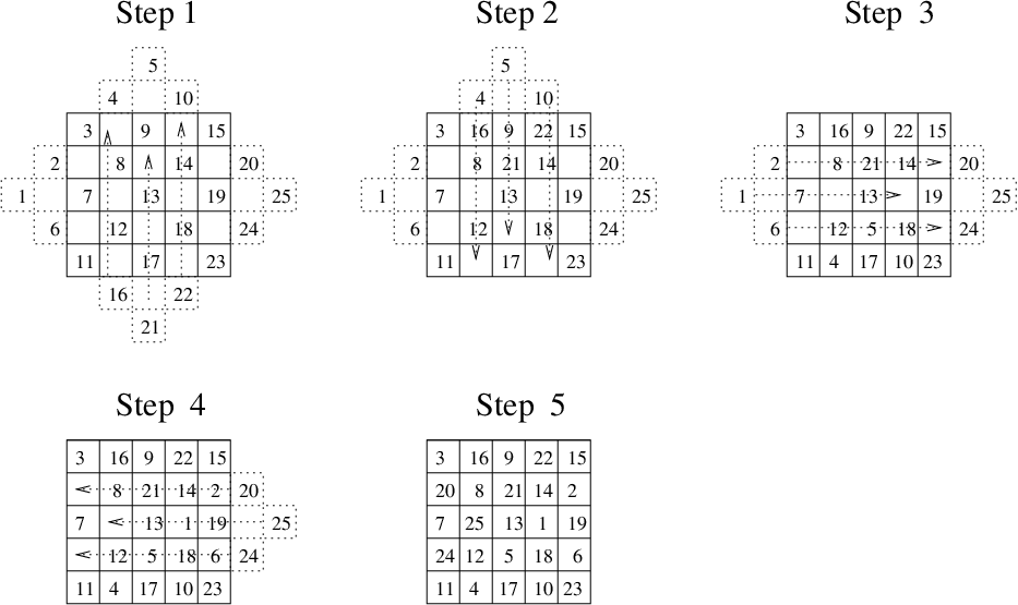
When the entries of an $n\times n$ magic square are $1,2,3,...,n^{2}$ , the magic square is called a pure magic square or a natural magic square. Methods for constructing natural magic squares are known for every order. One of my favorite methods of constructing a natural magic square with an odd number of cells is as follows: the numbers 1 to $n^{2}$ are written consecutively in diagonal columns as shown in Figure C.1. The numbers which are outside the center square are then transferred to the empty cells on the opposite sides of the latter without changing their order to get a magic square. This method is said to have been originated by Bachet de Meźiriac (see [7]).

A pair of numbers in the set $\{1,2,...,n^{2}\}$ which add to $n^{2}+1$ is called complementary. A method for constructing magic squares with an even number of cells using complementary pairs of numbers is as follows: write the number $1\dots n^{2}$ consecutively across rows. All entries except the numbers in the two main diagonals are then replaced by their complements to get a magic square (see Figure C.2). See [7] for details of these methods and other methods of constructing natural magic squares. For more recent developments in the construction of natural magic squares, see [13].

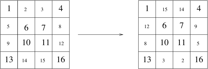
C.2 Other magic figures.

A composite magic square is a magic square composed of a series of small magic squares and an example is given in Table C.1. A concentric magic square is a magic square that remains a magic square with borders removed. An example of a modification of a concentric magic square devised by Frierson is shown in figure C.4.

71	64	69	8	1	6	53	46	51
66	68	70	3	5	7	48	50	52
67	72	65	4	9	2	49	54	47
26	19	24	44	37	42	62	55	60
21	23	25	39	41	43	57	59	61
22	27	20	40	45	38	58	63	56
35	28	33	80	73	78	17	10	15
30	32	34	75	77	79	12	14	16
31	36	29	76	81	74	13	18	11

Table C.1: A composite magic square [7].

A set of $n$ magic circles is a numbering of the intersections of the $n$ circles such that the sum over all intersections is the same constant for all circles. Consider the example of a die. It is commonly known that the opposite faces of a die contain complementary numbers that always add up to 7. Consequently any band of four numbers encircling a die gives a summation of 14 (see Figure C.5 A). These bands form magic circles (see Figures C.5 B or C.5 C). A magic sphere is a sphere that contains magic circles. The sphere in Figure C.5 A is a magic sphere.

A magic triangle is composed of three magic squares A, B, and C such that the square of any cell in C is equal to the sum of the squares of the corresponding cells in A and B. In other words the corresponding entries of the magic squares always form a Pythagorean triple ( $c^{2}=a^{2}+b^{2}$ ). C is called the hypotenuse, and A and B are called the legs of the magic triangle. An example is given in Figure C.6.

A magic star is a numbering of the intersections of a set of lines that form a star such that the sum over every intersection is the same for each line (see Figure C.7 for an example).

A magic carpet is a magic square in which a limited range of digits is used several times.

0	0	1	1
1	1	0	0
0	0	1	1
1	1	0	0

Table C.2: A magic carpet.

0	0	1	1	0	0	1	1
1	1	0	0	1	1	0	0
0	0	1	1	0	0	1	1
1	1	0	0	1	1	0	0
0	0	1	1	0	0	1	1
1	1	0	0	1	1	0	0
0	0	1	1	0	0	1	1
1	1	0	0	1	1	0	0

Table C.3: A magic carpet made from the magic carpet in Table C.2.

A magic rectangle is an $m\times n$ matrix such that all its rows add to a prescribed common sum, and all its columns add to the another prescribed sum. Therefore, a magic rectangle has two magic sums: A magic column sum and a magic row sum. Figure C.8 shows embeddings of magic squares in magic rectangles and vice versa and such patterns are called ornate magic squares ([7]).

See [7] for more examples of magic figures. Needless to say, we sure can construct and enumerate most of these magic figures with our methods.

Bibliography

[1] Alvis, D. and Kinyon, M. Birkhoff’s theorem for Panstochastic matrices, Amer. Math. Monthly, (2001), Vol 108, no.1, 28-37.
[2] Ahmed, M., De Loera, J., and Hemmecke, R., Polyhedral cones of magic cubes and squares, New Directions in Computational Geometry, The Goodman-Pollack Festschrift volume, Aronov et al., eds., Springer-Verlag, (2003), 25–41.
[3] Ahmed, M., How many squares are there, Mr. Franklin?: Constructing and Enumerating Franklin Squares, Amer. Math. Monthly, Vol. 111, 2004, 394–410.
[4] , Magic graphs and the faces of the Birkhoff polytope, arXiv:math.CO/0405181
[5] Alon, N. and Tarsi, M., A note on graph colorings and graph polynomials, J. Combin. Theory Ser. B 70 (1997), no. 1, 197–201.
[6] Anand, H., Dumir, V.C., and Gupta, H., A combinatorial distribution problem, Duke Math. J. 33, (1966), 757-769.
[7] Andrews, W. S., Magic Squares and Cubes, 2nd. ed., Dover, New York, 1960.
[8] Atiyah, M.F., and Macdonald, I.G., Introduction to Commutative Algebra, Addison-Wesley, Reading, MA, 1969.
[9] Ball, W.W.R. and Coxeter, H.S.M, Mathematical Recreations and Essays, 13th edition, Dover Publications, Inc, New York, 1987.
[10] Beck, M., The arithmetic of rational polytopes, Dissertation, Temple University (2000).
[11] Beck, M. and Pixton, D., The Ehrhart polynomial of the Birkhoff polytope, to appear in Discrete and computational geometry, Springer-Verlag, New York.
[12] Beck, M., Cohen, M., Cuomo, J., and Gribelyuk, P., The number of magic squares, cubes and hypercubes, Amer. Math. Monthly, 110, no.8, (2003), 707-717.
[13] Beck, M. and Zaslavsky, T., Inside-Out Polytopes, arXiv:math.CO/0309330.
[14] Bigatti, A.M., La Scala, R., and Robbiano, L., Computing toric ideals, J. Symbolic Computation, 27, (1999), 351-365.
[15] Bigatti, A.M, Computation of Hilbert-Poincaré Series, J. Pure Appl. Algebra, 119/3, (1997), 237–253.
[16] Billera, L.J. and Sarangarajan, A., The combinatorics of permutation polytopes, Formal power series and algebraic combinatorics (New Brunswick, NJ, 1994), 1–23, DIMACS Ser. Discrete Math. Theoret. Comput. Sci., 24, Amer. Math. Soc., Providence, RI, 1996.
[17] Bona, M., Sur l’enumeration des cubes magiques, C. R. Acad. Sci. Paris Ser. I Math., 316, (1993), no.7, 633-636.
[18] Brualdi, A. R. and Gibson, P., Convex polyhedra of doubly stochastic matrices: I, II, III, Journal of combinatorial Theory, A22, (1977), 467-477.
[19] Brualdi, A.R., Introductory combinatorics, 3 rd ed., Prentice hall, New Jersey, 1999.
[20] Bruns, W. and Koch, R., NORMALIZ, Computing normalizations of affine semigroups, Available via anonymous ftp from ftp//ftp.mathematik.uni-onabrueck.de/pub/osm/kommalg/software/
[21] Capani, A., Niesi, G., and Robbiano, L., CoCoA, A System for Doing Computations in Commutative Algebra, available via anonymous ftp from cocoa.dima.unige.it (2000).
[22] Carlitz, L., Enumeration of symmetric arrays, Duke Math. J., 33, (1966), 771-782.
[23] Chan, S. C. and Robbins, D. P., On the volume of the polytope of doubly stochastic matrices, Experiment. Math. 8 (1999), no.3, 291-300.
[24] Contejean, E. and Devie, H., Resolution de systemes lineaires d’equations diophantienes, C. R. Acad. Sci. Paris Sér. I Math., 313, (1991), no. 2, 115–120.
[25] Cox, D., Little, J., and O’Shea, D., Ideals, varieties, and Algorithms, Springer Verlag, Undergraduate Text, 2nd Edition, 1997.
[26] , Using Algebraic Geometry, Springer-Verlag, New York, 1998.
[27] De Loera, J., Hemmecke, R., Tauzer, J., and Yoshida, R., Effective lattice point counting in rational convex polytopes, to appear in the Journal of Symbolic Computation.
[28] De Loera, J.A. and Sturmfels, B., Algebraic unimodular counting, Algebraic and geometric methods in discrete optimization. Math. Program. 96 (2003), no. 2, Ser. B, 183–203.
[29] Dummit, D. S. and Foote, R. M., Abstract Algebra, Prentice Hall, New Jersey, 1991.
[30] Ehrhart, E., Sur un probléme de géométrie diophantienne linéaire II, J. Reine Angew. Math., 227, (1967), 25-49.
[31] , Figures magiques et methode des polyedres, J. Reine Angew. Math., 299/300, (1978), 51-63.
[32] , Sur les carrés magiques, C. R. Acad. Sci., Paris, 227 A, (1973), 575-577.
[33] Gardner, M., Martin Gardner’s New mathematical Diversions from Scientific American, Simon and Schuster, New York, (1966), 162-172.
[34] Giles, F.R. and Pulleyblank, W.R., Total dual integrality and integer polyhedra, Linear Algebra Appl., 25, (1979), 191-196.
[35] Gupta, H., Enumeration of symmetric matrices, Duke Math. J., 35, (1968), 653-659.
[36] Hagstorm R., Superlatively Regular $8\times 8$ Magic Squares, Personal communication (2004).
[37] Halleck, E.Q., Magic squares subclasses as linear Diophantine systems, Ph.D. dissertation, Univ. of California San Diego, (2000), 187 pages.
[38] Hemmecke, R., On the computation of Hilbert bases of cones, in Proceedings of First International Congress of Mathematical Software, A. M. Cohen, X.S. Gao, and N. Takayama, eds., Beijing, (2002); software implementation 4ti2 is available from http://www.4ti2.de.
[39] Henk, M. and Weismantel, R., On Hilbert bases of polyhedral cones, Results in Mathematics, 32, (1997), 298-303.
[40] Hilton, H., An introduction to the theory of groups of finite order, Oxford, 1908.
[41] König, D., Theory of finite and infinite graphs, Birkhäuser Boston, 1990.
[42] Lov́asz, L. and Plummer, M. D., Matching Theory, North-Holland, Amsterdam, 1986.
[43] MacMahon, P.A., Combinatorial Analysis, Chelsea, 1960.
[44] Pak, I., On the number of faces of certain transportation polytopes, European J. Combinatorics, vol. 21 (2000), 689-694.
[45] Pasles, P. C., The lost squares of Dr. Franklin: Ben Franklin’s missing squares and the secret of the magic circle, Amer. Math. Monthly, 108, (2001), 489-511.
[46] , Franklin’s other 8-square, J. Recreational Math., 31, (2003), 161-166.
[47] L. D. Patel, The secret of Franklin’s $8\times 8$ magic square, J.Recreational Math., 23, (1991), 175-182.
[48] Pickover, C.A., The Zen of magic squares, circles, and stars, Princeton University Press, New Jersey, 2002.
[49] Pottier, L., Bornes et algorithme de calcul des générateurs des solutions de systémes diophantiens linéaires, C. R. Acad. Sci. Paris, 311, (1990), no. 12, 813-816.
[50] Pottier, L., Minimal solutions of linear Diophantine systems: bounds and algorithms, in Rewriting techniques and applications (Como, 1991), 162–173, Lecture Notes in Comput. Sci., 488, Springer, Berlin, 1991.
[51] Schrijver, A., Theory of Linear and Integer Programming, Wiley-Interscience, 1986.
[52] Schubert, H., Mathematical Essays and Recreations, The open Court Publishing Co., 1899.
[53] Stanley, R.P., Enumerative Combinatorics, Volume I, Cambridge, 1997.
[54] , Combinatorics and commutative algebra, Progress in Mathematics, 41, Birkhaüser Boston, MA, 1983.
[55] ) , Linear Homogeneous Diophantine Equations and Magic Labelings Of Graphs, Duke Mathematical Journal, Vol. 40, September 1973, 607-632.
[56] , Magic Labelings of Graphs, Symmetric Magic Squares, Systems of Parameters and Cohen-Macaulay Rings, Duke Mathematical Journal, Vol. 43, No.3, September 1976, 511-531.
[57] Stewart, B. M., Magic graphs, Canad. J. Math., vol. 18, (1966), 1031-1059.
[58] , Supermagic complete graphs, Canad. J. Math., vol. 19, (1967), 427-438.
[59] Sturmfels, B., Algorithms in invariant theory, Springer-Verlag, Vienna, 1993.
[60] , Gröbner Bases and Convex Polytopes, University Lecture Series, no. 8, American Mathematical Society, Providence, 1996.
[61] Thiéry, N. M., Algebraic invariants of graphs; a study based on computer exploration, SIGSAM Bulletin (2000), 9-20.
[62] Wallis, D., Magic Graphs, Birkhäuser Boston, 2001.
[63] Van Lint, J.H. and Wilson, R.M., A course in Combinatorics, 2 nd edition, Cambridge University Press, Cambridge, 2001.
[64] Vergne, M. and Baldoni-Silva, W., Residues formulae for volumes and Ehrhart polynomials of convex polytopes, manuscript 81 pages available at math.ArXiv, CO/0103097.

71	64	69	8	1	6	53	46	51
66	68	70	3	5	7	48	50	52
67	72	65	4	9	2	49	54	47
26	19	24	44	37	42	62	55	60
21	23	25	39	41	43	57	59	61
22	27	20	40	45	38	58	63	56
35	28	33	80	73	78	17	10	15
30	32	34	75	77	79	12	14	16
31	36	29	76	81	74	13	18	11

0	0	1	1	0	0	1	1
1	1	0	0	1	1	0	0
0	0	1	1	0	0	1	1
1	1	0	0	1	1	0	0
0	0	1	1	0	0	1	1
1	1	0	0	1	1	0	0
0	0	1	1	0	0	1	1
1	1	0	0	1	1	0	0

71	64	69	8	1	6	53	46	51
66	68	70	3	5	7	48	50	52
67	72	65	4	9	2	49	54	47
26	19	24	44	37	42	62	55	60
21	23	25	39	41	43	57	59	61
22	27	20	40	45	38	58	63	56
35	28	33	80	73	78	17	10	15
30	32	34	75	77	79	12	14	16
31	36	29	76	81	74	13	18	11

0	0	1	1	0	0	1	1
1	1	0	0	1	1	0	0
0	0	1	1	0	0	1	1
1	1	0	0	1	1	0	0
0	0	1	1	0	0	1	1
1	1	0	0	1	1	0	0
0	0	1	1	0	0	1	1
1	1	0	0	1	1	0	0