Quasi-actions on trees II:
Finite depth Bass-Serre trees

Lee Mosher Thanks: Supported in part by NSF grant DMS 0103208. Michah Sageev Kevin Whyte Thanks: Supported in part by NSF grant DMS 0204576

Abstract

This paper addresses questions of quasi-isometric rigidity and classification for fundamental groups of finite graphs of groups, under the assumption that the Bass-Serre tree of the graph of groups has finite depth. The main example of a finite depth graph of groups is one whose vertex and edge groups are coarse Poincare duality groups. The main theorem says that, under certain hypotheses, if ${\mathcal{G}}$ is a finite graph of coarse Poincare duality groups then any finitely generated group quasi-isometric to the fundamental group of ${\mathcal{G}}$ is also the fundamental group of a finite graph of coarse Poincare duality groups, and any quasi-isometry between two such groups must coarsely preserves the vertex and edge spaces of their Bass-Serre trees of spaces. Besides some simple normalization hypotheses, the main hypothesis is the “crossing graph condition”, which is imposed on each vertex group ${\mathcal{G}}_{v}$ which is an $n$ -dimensional coarse Poincare duality group for which every incident edge group has positive codimension: the crossing graph of ${\mathcal{G}}_{v}$ is a graph $\epsilon_{v}$ that describes the pattern in which the codimension 1 edge groups incident to ${\mathcal{G}}_{v}$ are crossed by other edge groups incident to ${\mathcal{G}}_{v}$ , and the crossing graph condition requires that $\epsilon_{v}$ be connected or empty.

1 Introduction

One important part of geometric group theory is the classification of finitely generated groups up to quasi-isometry. This paper addresses that question for many groups which split as graphs of groups. A typical question in this context is: suppose $G$ splits as a graph of groups and $H$ is quasi-isometric to $G$ , must $H$ split in a similar way?

The first example of this type is Stallings Ends Theorem, which implies that if $G$ splits with finite edge groups, then so must $H$ . This result was recently refined in work of Papasoglu and Whyte [PW02] which implies that if $G$ and $H$ are accessible groups then they have the same quasi-isometry types of one-ended factors. After Stallings theorem, the next result of this type came in work of Kapovich and Leeb [KL97] which shows that if $M$ is a Haken $3$ -manifold then the splitting of $\pi_{1}(M)$ induced by the geometric decomposition of $M$ is preserved by quasi-isometries. Farb and Mosher [FM99] showed that if $G$ splits as a graph of ${\mathbf{Z}}$ ’s with solvable fundamental group — a solvable Baumslag-Solitar group — then so must $H$ up to finite groups. Papasoglu [Pap05] showed that if $G$ splits with two-ended edge groups, then $H$ must as well. Mosher, Sageev and Whyte [MSW03] showed that if $G$ splits as a “bushy” graph of coarse Poincaré duality groups of constant dimension, then so must $H$ .

Not all splittings exhibit this type of rigidity. For instance, cocompact lattices in $\SL(2,{\mathbf{R}})\times\SL(2,{\mathbf{R}})$ are all quasi-isometric, however, by a theorem of Margulis the irreducible ones do not split while reducible ones split as amalgams in a myriad of ways ([Mar81], and see also [MS04]).

In this paper, we focus on graphs of groups whose vertex groups are “manifold-like”, for example fundamental groups of closed aspherical manifolds, and more generally finitely presented Poincaré duality groups. Since we are dealing with quasi-isometry issues, it turns out that the natural class of groups to work with are coarse Poincaré duality groups, introduced by Kapovich and Kleiner [KK99]. In a previous paper [MSW03] we studied a special case in which all of the vertex and edge groups have the same dimension, equivalently, every edge-to-vertex injection in the graph of groups has finite index image; such graphs of groups are called (geometrically) homogeneous. In this paper, we address more general cases.

Papasoglu’s preprint [Pap02] independently studies graphs of groups with a similar focus and overlapping results to ours; we explain below some of the similarities and differences of our approaches and results.

The main theorems 1.5, 1.6 and 1.7 are somewhat involved, so before launching into a full discussion of them, we begin with some applications, chosen from among the gamut of settings to which the main theorems apply.¹¹ 1 The main theorems, and several of the applications, were announced in [MSW00].

1.1 Example applications

First, here is a theorem regarding two fundamental groups of hyperbolic manifolds amalgamated along infinite cyclic subgroups. For the proof see Theorem 7.1, which relies essentially on a theorem of Schwartz [Sch97].

Theorem 1.1.

Let $A$ and $B$ be fundamental groups of closed hyperbolic manifolds of dimension at least $3$ , and let $G$ be the amalgamated free product $A*_{\mathbf{Z}}B$ where ${\mathbf{Z}}$ includes as a maximal cyclic subgroup in both $A$ and $B$ . If $H$ is a finitely generated group quasi-isometric to $G$ then $H$ splits as a graph of groups each of whose vertex groups is commensurable to $A$ or $B$ . In particular, there are infinitely many quasi-isometry classes of groups of this form.

In fact, in the context of Theorem 1.1 one obtains a complete computation of the quasi-isometry group; see Proposition 7.13.

Notice that in the above example, the vertex-to-edge inclusions are codimension-2. As we will see below, Alexander duality can be applied in a straightforward manner. In the codimension-1 setting, one typically needs that the edge subgroups in a vertex group cross one another in some suitable sense. Here is one such example.

A collection of geodesics in the hyperbolic plane is said to be filling if the complementary regions are all bounded. A collection of cyclic subgroups in a surface group is said to be filling if the pattern of geodesics in the universal cover is filling.

Theorem 1.2.

Suppose that $G$ splits as a graph of groups where each vertex group is a surface group, each edge group is a cyclic group and the edge-to-vertex inclusions provide a filling collection of curves on the vertex group. Then any torsion-free group quasi-isometric to $H$ splits as a graph of groups whose edge groups are cyclic and whose vertex groups are surface groups or cyclic groups.

A stronger version of Theorem 1.2 is given in Theorem 7.8, with commensurability information built into the conclusion, by applying a theorem of Kapovich and Kleiner [KK00]. Using this we will obtain infinitely many distinct quasi-isometry classes of groups of this type.

The next theorem gives examples with higher dimensional edge groups, namely fundamental groups of surfaces. For the proof see Theorem 7.4, and for even stronger rigidity conclusions in many examples see Theorem 7.14.

Theorem 1.3.

Let $A$ be the fundamental group of a hyperbolic $3$ -manifold which fibers over the circle in two ways, with fibers $F_{1}$ and $F_{2}$ . Let $\phi$ be any isomorphism between (finite index subgroups of) $\pi_{1}(F_{1})$ and $\pi_{1}(F_{2})$ and define $G$ as the HNN extension $A*_{\phi}$ . If $H$ is any torsion free group quasi-isometric to $G$ , then $H$ splits as a graph of groups, whose edge groups are surface groups, and whose vertex groups are hyperbolic 3-manifold groups commensurable to $A$ and surface groups.

The commensurability information in Theorem 1.3 is an application of a theorem of Farb and Mosher [FM02b].

Here is a theorem for abelian groups.

Theorem 1.4.

Suppose $A$ is a finitely generated abelian group of rank $n$ , $G_{1},G_{2}<A$ are two rank $n-1$ subgroups that span $A$ , and $G$ is an HNN-extension identifying $G_{1}$ to $G_{2}$ . Then any group $H$ quasi-isometric to $G$ splits as a graph of virtually abelian groups with edge groups of rank $n-1$ and vertex groups of rank at most $n$ .

A much more general result is given in Corollary 7.11, applying to a broad spectrum of graphs of abelian groups.

1.2 The methods of proof: a special case.

We illustrate some of the ideas involved in proving our main theorems by sketching the proof in the special case of theorem 1.1. Let $M$ and $N$ be closed hyperbolic $n$ -manifolds for some $n\geq 3$ . Let $A$ and $B$ be their fundamental groups. Choosing maximal cyclic subgroups of $A$ and $B$ amounts to choosing primitive closed geodesics in $M$ and $N$ . Let $Y$ be the space built by gluing an annulus to $M$ and $N$ , with the boundary circles attached to the chosen geodesics. The group $G=A*_{\mathbf{Z}}B$ is $\pi_{1}(Y)$ , and so acts properly discontinuously and cocompactly on $X=\widetilde{Y}$ . The space $X$ is built from copies of ${\mathbf{H}}^{n}$ glued together with strips attached along the geodesics which cover the chosen curves in $M$ and $N$ . There is a natural $G$ -equivariant map, $\pi:X\to T$ , from $X$ to the Bass-Serre tree $T$ of the splitting of $G$ in which each copy of ${\mathbf{H}}^{n}$ is mapped to a single vertex, and each strip maps to an edge. The is an example of what we call a Bass-Serre complex, which serves as the standard model space for our considerations. (See Section 2.4 for the general construction.) We call the copies of ${\mathbf{H}}^{n}$ in $X$ the vertex spaces $X_{v}$ , one for each vertex $v\in T$ . The strips are called the edge spaces $X_{e}$ , one for each edge $e\subset T$ .

We start by understanding the self quasi-isometries of $G$ . This is typically a crucial step in proving rigidity results. The salient point is that a quasi-isometry from some mystery group $H$ to $G$ provides a natural map from $H$ to $\QI(G)$ , the quasi-isometry group of $G$ . Thus one seeks geometric patterns which are invariant under $\QI(G)$ . As $X$ is quasi-isometric to $G$ , we can work with quasi-isometries of $X$ . Since $X$ is uniformly contractible, we can move any quasi-isometry a bounded distance to a continuous map. Let $f\colon X\to X$ be such a continuous quasi-isometry. Our method of proof consists of two main steps.

Step 1 – Vertex Rigidity:

There is an $R>0$ such that for any vertex space $X_{v}\subset X$ there is a vertex space $X_{v^{\prime}}\subset X$ with $d_{\mathcal{H}}(f(X_{v}),X_{v^{\prime}})\leq R$ , where $d_{\mathcal{H}}(\cdot,\cdot)$ denotes the Hausdorff metric.

Step 2 – Tree Rigidity:

There is a automorphism $\tau$ of $T$ and a quasi-isometry $f^{\prime}\colon X\to X$ at bounded distance from $f$ such that $\pi\circ f^{\prime}=\tau\circ\pi$ .

Conclusion:

If we establish steps 1 and 2, then we may conclude that if $H$ is quasi-isometric to $G$ then $H$ acts on $T$ with finite quotient; for every vertex $v$ of $T$ , $H_{v}$ is quasi-isometric to $G_{v}$ and similarly, for every edge $e$ , $H_{e}$ is quasi-isometric to $G_{e}$ . In particular, $H$ has a splitting as a graph of groups with virtually cyclic edge groups and vertex groups quasi-isometric to ${\mathbf{H}}^{3}$ . A theorem of Schwartz [Sch97] then tells us that the vertex and edge groups of the splitting for $H$ are commensurable to the corresponding ones for $G$ .

Let us now see how steps 1 and 2 are proven in this setting.

Vertex rigidity.

Suppose that vertex rigidity fails. Then one finds an edge space $X_{e}$ such that $f(X_{v})$ travels deeply into both complementary components of $X_{e}$ . This will implies that $X_{e}$ (which we recall is quasi-isometric to a line) coarsely separates $f(X_{v})$ . But now note that $f(X_{v})$ is quasi-isometric to ${\mathbf{H}}^{n}$ , so we get a subset of a line coarsely separating ${\mathbf{H}}^{n}$ with $n\geq 3$ . This contradicts a coarse version of Alexander duality.

Tree rigidity.

The vertex rigidity step yields a bijection $f_{\#}\colon\Vertices(T)\to\Vertices(T)$ , so that $f(X_{v})$ has finite Hausdorff distance from $X_{f_{\#}{(v)}}$ . We now wish to see that $f$ carries neighboring vertex spaces to neighboring vertex spaces. The key point here is that in $X$ , adjacent vertex spaces are characterized coarsely by the fact that they have neighborhoods with unbounded intersection, whereas any intersection of neighborhoods of non-adjacent vertex spaces is bounded. This fact relies on the assumption that the cyclic edge groups are maximal in their respective vertex spaces. Thus $f_{\#}$ carries adjacent vertices to adjacent vertices and hence extends to an isometry $\tau$ of $T$ as required.

1.3 The general setting

The proofs of our main theorems for more general graphs of groups follow a similar outline. Let us discuss some of the issues that arise in the more general setting, and the various hypotheses needed to deal with these issues.

For starters, our graphs of groups ${\mathcal{G}}$ will always satisfy the standard hypothesis of irreducibility, meaning that for every edge of ${\mathcal{G}}$ with distinct endpoints, both of its edge-to-vertex injections have image of index $\geq 2$ . Every finite graph of groups can be made irreducible by inductively collapsing edges, without changing the fundamental group.

Let $T$ denote the Bass-Serre tree of ${\mathcal{G}}$ , and let $X$ denote the Bass-Serre complex of ${\mathcal{G}}$ . The group $\pi_{1}{\mathcal{G}}$ acts on $X$ and $T$ , and there is a $\pi_{1}{\mathcal{G}}$ equivariant projection map $X\to T$ . The action on $X$ is properly discontinuous and cocompact, and the action on $T$ is cocompact with quotient graph of groups ${\mathcal{G}}$ . The inverse image under the projection map $X\to T$ of a vertex $v\in T$ is a vertex space denoted $X_{v}$ , and the inverse image of the midpoint of an edge $e\subset T$ is an edge space denoted $X_{e}$ .

Vertex Rigidity.

The proof of the vertex rigidity step in Section 1.2 above relied on the fact that no geodesic can coarsely separate ${\mathbf{H}}^{n}$ when $n\geq 3$ . In general we want to know that edge spaces cannot disconnect vertex spaces. In most applications the essential focus is on the maximal vertex spaces, those not strictly coarsely contained in any other vertex space. We call these the depth zero vertex spaces. An important hypothesis of our results will be that every vertex space is coarsely contained in a depth zero vertex space.

To see that edge spaces cannot coarsely separate the depth zero vertex spaces we generally use a coarse version of Alexander duality to understand the separation properties of subsets. The right context for these arguments is that of coarse Poincare duality spaces introduced in [KK99]. Almost all of our results assume that the depth zero vertex spaces are coarse $\PD$ spaces (see section 2.6 for detailed definitions). To put it another way, the stabilizer groups of depth zero vertices are required to be “coarse $\PD$ groups”. This is an essential hypothesis for all of our results.

There are several different vertex rigidity phenomena. For example, given a coarse $\PD(n)$ vertex space, if the incident edge spaces are of dimension at most $n-2$ then we can use a version of the vertex rigidity step of Section 1.2: in a coarse $\PD(n)$ space, no subspace whose “coarse codimension” is $\geq 2$ can coarsely separate the ambient space. We must also study vertex rigidity phenomena in the presence of incident edge spaces of coarse codimension zero and one. In order to make sense of these different phenomena, for example in order for the coarse codimension of an edge space in a vertex space to be well-defined, we will add a hypothesis that the edge spaces satisfy a coarse version of the finite type property. In other words, the stabilizers of edges (and also of positive depth vertices) are required to be “coarse finite type groups” (see section 2.6). The coarse finite type hypothesis is a convenient assumption for our results, although not essential like the coarse $\PD$ assumption; see the comments after the statement of Proposition 3.16.

Continuing with a discussion of vertex rigidity phenomena, a codimension zero inclusion corresponds to an edge group which has finite index in the vertex group. A depth zero raft $R$ is a maximal subtree of the Bass-Serre tree whose vertices have depth zero, and whose edge stabilizers include with finite index in incident vertex stabilizers. The union of vertex and edge spaces corresponding to vertices and edges in $R$ is a portion of the Bass-Serre complex $X$ called a raft space denoted $X_{R}$ . A depth zero raft $R$ is a Bass-Serre tree for a geometrically homogeneous graphs of groups, whose fundamental group is the stabilizer of the raft, and the raft space $X_{R}$ is the corresponding Bass-Serre complex. We can use our previous results [MSW03] to study depth zero rafts. Those results apply to give vertex rigidiy for a geometrically homogeneous graph of coarse $\PD(n)$ groups, but only when its Bass-Serre tree is not a line. That means we must add a hypothesis that no depth zero raft is a line, equivalently, each depth zero raft is either a point or a bushy tree (see Proposition 2.6).

Codimension one edges also require certain additional hypotheses. To explain these assumptions, consider the group $F_{2}\times{\mathbf{Z}}\approx\langle b,t\rangle\times\langle a\rangle$ , which splits as an HNN amalgamation of ${\mathbf{Z}}\oplus{\mathbf{Z}}\approx\langle a,b\rangle$ over a cyclic group, with stable letter $t$ — that is, $\langle a,b,t\bigm|[a,b]=1,a^{t}=a\rangle$ . The Bass-Serre complex $X$ of this splitting does not satisfy vertex rigidity: the automorphism $b\mapsto t$ , $t\mapsto b$ , $a\mapsto a$ fails to respect the vertex spaces of $X$ . This failure stems from the fact each edge space $X_{e}$ coarsely separates each incident vertex space $X_{v}$ in $X$ — that is, for any sufficiently large neighborhood of $X_{e}$ in $X$ , the set $X_{v}$ enters deeply into two distinct complementary components of this neighborhood.

In order to avoid this problem, we introduce the crossing graph condition. Consider a coarse $\PD(n)$ vertex space $X_{v}$ of depth zero which is not coarsely equivalent to any other vertex space; equivalently, the vertex $v$ is a depth zero raft of the Bass-Serre tree. Define the crossing graph of $X_{v}$ to be a graph $\epsilon_{v}$ with one vertex for each coarse $\PD(n-1)$ edge space incident to $X_{v}$ , and with edges as follows. If $X_{e}$ is a coarse $\PD(n-1)$ edge space incident to $X_{v}$ , then a subset $A\subset X_{v}$ is said to cross $X_{e}$ in $X_{v}$ if $A$ goes deeply into both complementary components of $X_{v}-X_{e}$ ; see Sections 2.1 and 3.1 for details on crossing. Consider two vertices $X_{e}$ , $X_{e^{\prime}}$ of $\epsilon_{v}$ . We connect these vertices by an edge of $\epsilon_{v}$ if one of two things happens: either there is an another edge $e^{\prime\prime}$ incident to $v$ (with no restriction on the dimension of $X_{e^{\prime\prime}}$ ) such that $X_{e^{\prime\prime}}$ crosses both $X_{e}$ and $X_{e^{\prime}}$ in $X_{v}$ ; or $X_{e}$ and $X_{e^{\prime}}$ cross each other in $X_{v}$ .

Crossing graph condition:

For each $n$ , and for each depth zero vertex $v$ which is a raft and whose vertex space $X_{v}$ is coarse $\PD(n)$ ,

1.

For any edge $e$ incident to $v$ , if the edge space $X_{e}$ coarsely separates $X_{v}$ then $X_{e}$ is coarse $\PD(n-1)$ .
2.

The crossing graph $\epsilon_{v}$ is connected or empty.

Crossing graphs have been used before in geometric group theory. For example, in the proof of the algebraic torus theorem of Dunwoody and Swenson [DS00], a crossing graph similar to ours is constructed and its connectivity properties are used in the proof, although their crossing graph allows an edge only when two codimension 1 subspaces cross each other and not when they are both crossed by a third subspace.

Here are two good examples to keep in mind. First, for vertex group ${\mathbf{Z}}^{n}$ , connectedness of the crossing graph condition is equivalent to the assumption that the edge groups rationally span the vertex group. The second example is a surface group as the vertex group, with edge groups ${\mathbf{Z}}$ . Connectedness of the crossing graph means that the curves corresponding to the edge groups fill the surface.

To summarize, here are the key hypotheses designed to guarantee depth zero vertex rigidity, as given in our general depth zero vertex rigidity theorem 2.10:

•

All depth zero vertices are coarse $\PD$ .
•

No depth zero raft is a line.
•

The crossing graph condition holds.

Another convenient hypothesis, designed to make various concepts of dimension well defined, is:

•

Each vertex and edge group is coarse finite type.

Tree Rigidity.

In the proof of Theorem 1.1 we identified the tree using the coarse intersections of the vertex spaces. In general this is not possible. For example, in the free product of two groups $G=A*B$ , the coarse intersection of any pair of vertex spaces is bounded, so there is no direct way to reconstruct the tree. Indeed, $G$ has many quasi-isometries which do not arise from tree automorphisms. A similar situation occurs if one tries to extend Theorem 1.1 to cover amalgamations over non-maximal cyclic subgroups. In order to control the complexity of the coarse inclusion lattice of edge spaces, we introduce the following:

Finite depth hypothesis: There is a bound on the length of a chain of strict coarse inclusions of edge spaces.

When this hypothesis is satisfied we say that ${\mathcal{G}}$ , or its Bass-Serre tree $T$ , have finite depth. See Section 4 for details. It turns out that in the setting of graphs of groups with coarse $\PD$ vertex and edge groups, the finite depth hypothesis is always satisfied. When the depth zero vertices are required to be coarse $\PD$ , but not the remaining edge and vertex groups, then the finite depth hypothesis may or may not be satisfied.

The finite depth hypothesis can be thought of as a way to tame the coarse inclusion lattice of edge spaces, and it plays a key role in reconstructing a tree structure, as needed to prove tree rigidity.

The general statement of tree rigidity is given in Theorem 2.12.

Here is an intriguing example, which highlights the limitations of our techniques. Let $K$ be a $\PD(n)$ group with a free subgroup, let $\phi\colon A\to B$ be an isomorphism between two free subgroups of $K$ of rank $\geq 2$ , and consider the HNN amalgamation $G=K*_{\phi}$ . Let $T$ be the Bass-Serre tree of $G$ . Suppose that $B$ has infinite index in $A$ , or suppose that one of the subgroups $A$ or $B$ is conjugate in $K$ to an infinite index subgroup of itself. In this case there exists a bi-infinite sequence of edges $\ldots,e_{-1},e_{0},e_{1},\ldots$ in $T$ such that if $G^{e_{i}}$ denotes the subgroup of $G$ stabilizing $e_{i}$ then each $G^{e_{i}}$ is an infinite index subgroup of $G^{e_{i+1}}$ . In other words, the Bass-Serre complex has infinite depth. Our techniques do not apply in this situation: if $H$ is quasi-isometric to $G$ then we cannot conclude using our techniques that $H$ splits as the fundamental group of a graph of groups with coarse $\PD(n)$ vertex groups and virtually free edge groups. Nonetheless, there are two partial results in this situation: our vertex rigidity theorem 2.10 does apply provided $n\geq 3$ , and it shows that $H$ has subgroups corresponding to the vertex groups of $G$ ; and on the other hand Papasoglu’s results in [Pap02] apply to show that $H$ splits over a virtually free group. We have not investigated how to combine these results; in particular, we do not know how to get complete control over a graph of groups for $H$ in the manner of our main quasi-isometric rigidity theorem 1.5.

1.4 Statements of results

We now give full statements of our main results on quasi-isometric rigidity and classification, together with an application to graphs of coarse $\PD$ groups that generalizes all of the examples of Section 1.1. The graphs of groups ${\mathcal{G}}$ to which our theorems apply are characterized by the following hypotheses:

(1)

${\mathcal{G}}$ is finite type, irreducible, and of finite depth.
(2)

No depth zero raft of the Bass-Serre tree of ${\mathcal{G}}$ is a line.
(3)

Every depth zero vertex group of ${\mathcal{G}}$ is coarse $\PD$ .
(4)

For every one vertex, depth zero raft of the Bass-Serre tree, the crossing graph condition holds.
(5)

Every vertex and edge group is coarse finite type.

Theorem 1.5 (Quasi-isometric rigidity theorem).

Let ${\mathcal{G}}$ be a graph of groups satisfying (1)–(5) above. If $H$ is a finitely generated group quasi-isometric to $\pi_{1}{\mathcal{G}}$ then $H$ is the fundamental group of a graph of groups satisfying (1–5) above.

In studying the large scale geometry of groups, besides proving that a particular class of groups is closed under quasi-isometry (rigidity), one wants to obtain a complete classification up to quasi-isometry of the groups in that class. In the present situation, our class of groups is too broadly defined to expect a complete classification. We will settle for reducing the classification of the whole group to classification of the vertex and edge groups and the pattern in which those groups are pieced together. There are many examples where one can go further and get a complete classification of a specific class of groups that is closed up to quasi-isometry: in the geometrically homogeneous case see [FM98], [Why02], [FM00], [FM02b], [Why04a]; and in the inhomogeneous case see Theorem 7.2 above and other examples in Section 7.

To state the Classification Theorem, consider a graph of groups ${\mathcal{G}}$ with Bass-Serre tree of spaces $X\to T$ . Let $\VE(T)=V(T)\cup E(T)$ , where the usual simplicial metric on $T$ induces a metric on $\VE(T)$ by representing each edge $e\in E(T)$ by its midpoint.

Theorem 1.6 (Quasi-isometric classification theorem).

Let ${\mathcal{G}},{\mathcal{G}}^{\prime}$ be graphs of groups satisfying (1–5) above. Let $X\to T$ , $X^{\prime}\to T^{\prime}$ be Bass-Serre trees of spaces for ${\mathcal{G}},{\mathcal{G}}^{\prime}$ , respectively. If $f\colon X\to X^{\prime}$ is a quasi-isometry then $f$ coarsely respects vertex and edge spaces. To be precise, for any $K\geq 1$ , $C\geq 0$ there exists $K^{\prime}\geq 1$ , $C^{\prime}\geq 0$ such that if $f\colon X\to X^{\prime}$ is a $K,C$ quasi-isometry then there exists a $K^{\prime},C^{\prime}$ quasi-isometry $f_{\#}\colon\VE(T)\to\VE(T^{\prime})$ such that the following hold:

•

If $a\in\VE(T)$ then $d_{\mathcal{H}}(f(X_{a}),X^{\prime}_{f_{\#}(a)})\leq C^{\prime}$ .
•

If $a^{\prime}\in\VE(T^{\prime})$ then there exists $a\in\VE(T)$ such that $d_{\mathcal{H}}(f(X_{a}),X^{\prime}_{a^{\prime}})\leq C^{\prime}$ .

The finite depth hypothesis insures that $T,T^{\prime}$ each have a nonempty collection of depth zero rafts, and so in particular this theorem says that $f$ induces a bijection between the depth zero rafts of $T$ and of $T^{\prime}$ .

The conclusion of Theorem 1.6 embraces several further conclusions. For example, if $a\in\VE(T)$ and $a^{\prime}=f_{\#}(a)\in\VE(T)$ then $f$ induces a quasi-isometry between the subgroup of $\pi_{1}{\mathcal{G}}$ stabilizing $a$ and the subgroup of $\pi_{1}{\mathcal{G}}^{\prime}$ stabilizing $b$ . Somewhat deeper implications arise from considering adjacencies of vertex and edge spaces, for example the conclusion about edge group patterns in a vertex group in Corollary 7.2. We will explore this more in Section 7 under the moniker of “pattern rigidity”.

Graphs of coarse Poincaré duality groups.

If $G$ is a coarse $\PD(n)$ group and $H\subset G$ is a coarse $\PD(k)$ subgroup then $k\leq n$ , with strict inequality if and only if $H$ has infinite index in $G$ . This is well known fact for ordinary Poincaré duality groups [Bro82], and the generalization to coarse Poincaré duality groups is due to Kapovich and Kleiner ([KK99], see also Lemma 3.12).

Suppose now that ${\mathcal{G}}$ is any finite graph of coarse $\PD$ groups. The fact just noted about dimensions of subgroups shows that ${\mathcal{G}}$ has finite depth. We can therefore apply Theorems 1.5 and 1.6 to ${\mathcal{G}}$ , obtaining the following theorem which applies, for example, to all of the examples considered in Section 1.1:

Theorem 1.7 (QI Rigidity and Classification for graphs of coarse $\PD$ groups).

Let ${\mathcal{G}}$ be a finite, irreducible graph of coarse Poincaré duality groups satisfying (2) and (4): no depth zero raft of the Bass-Serre tree $T$ is a line; and the crossing graph condition holds for every one vertex depth zero raft of $T$ . If $H$ is any finitely generated group quasi-isometric to $\pi_{1}{\mathcal{G}}$ then $H$ is the fundamental group of a finite type, irreducible graph of coarse Poincaré duality groups ${\mathcal{G}}^{\prime}$ satisfying (2) and (4). Furthermore, for any such ${\mathcal{G}}^{\prime}$ , any quasi-isometry $\pi_{1}{\mathcal{G}}\to\pi_{1}{\mathcal{G}}^{\prime}$ coarsely respects vertex and edge spaces.

As explained at the end of Section 6, two of the hypotheses — irreducibility, and no depth zero raft is a line — are normalization hypotheses: given any finite graph of $\PD$ groups, the graph can be normalized in a canonical way so as to make these two hypotheses true, without changing the fundamental group, and changing the vertex and edge stabilizers in a predictable way. The most important and restrictive hypothesis is therefore the crossing graph hypothesis. The theorem applies to any (normalized) finite graph of coarse Poincaré duality groups subject to the crossing graph hypothesis.

There are other situations outside of the coarse $\PD$ world to which Theorems 1.5 and 1.6 apply, although verifying the finite depth hypothesis can become tricky; see the end of Section 7.2 for one such class of examples.

Relations with work of Papasoglu.

Our results have some overlap with Papasoglu’s paper [Pap02], but with somewhat different goals. In particular, many of the special examples in Section 1.1 above are handled in Papasoglu’s paper as well.

The main difference between the two papers is that the results of [Pap02] are focussed not on the overall structure of a graph of groups, but on the question of whether a group splits with a given type of edge group. As such, the hypotheses of the results in [Pap02] are generally weaker than ours, and so have wider applicability. On the other hand, the conclusions are also weaker.

To compare the techniques, the use of coarse Alexander duality to understand vertex groups is similar here and in [Pap02]. On the other hand, the splittings in [Pap02] are obtained in a different manner, by applying work of Dunwoody and Swenson [DS00].

1.5 Structure of the paper

In Section 2 we introduce the basic notions of coarse geometry, Bass-Serre theory, and the coarse separation properties which we will need, including a discussion of coarse Poincaré duality groups. All concepts introduced in this introduction are carefully developed in Section 2.

Also, in Section 2.7 we introduce the overall scheme of the proofs of the main theorems. The proofs are broken into three steps. The first step is the Depth Zero Vertex Rigidity Theorem 2.10. The second step, which was suppressed in our earlier discussion, is the Vertex–Edge Rigidity Theorem 2.11; this result gives rigidity for vertex and edge spaces of arbitrary depth, starting from a hypothesis of depth zero vertex rigidity. The third step is the Tree Rigidity Theorem 2.12.

In Section 3 we prove Depth Zero Vertex Rigidity 2.10. First we prove rigidity for the depth zero rafts, and then we apply geometrically homogeneous methods (e.g. [FM00] or [MSW03]) to establish vertex rigidity within the rafts.

In Section 4 we explore the coarse lattice of vertex and edge spaces, with respect to the operations of coarse set theory, in order to prove Vertex—Edge Tigidity 2.11. This coarse lattice structure organizes the coarse equivalence classes of vertex and edge spaces into rafts of higher depth.

Section 5 proves the Tree Rigidity Theorem 2.12. With the results of the previous sections already established, at this point we may conclude that quasi-isometries on the Bass-Serre complex descend to quasi-isometries on the Bass-Serre tree. Thus, a mystery group $H$ quasi-isometric to the Bass-Serre complex $X$ quasi-acts on the Bass-Serre tree $T$ . In Section 5 we show how to use the coarse lattice structure, together with Dunwoody’s theory of tracks, in order to produce an action of $H$ on a tree $T^{\prime}$ quasiconjugate to the quasi-action of $H$ on $T$ . This gives the desired splitting of $H$ .

In Section 6 we put together the results of Sections 3, 4, and 5 to prove the main quasi-isometric rigidity Theorem 1.5. We also prove the main quasi-isometric classification Theorem 1.6, using only the results of Section 3 and 5; tree rigidity is not needed. We also apply these results to a very broad spectrum of graphs of coarse Poincaré duality groups; see Theorem 1.7.

Finally in Section 7 we restrict our discussion to some interesting special cases, including all of the example applications from above. Together with some pattern rigidity results (including deep work of R. Schwartz), we obtain some stronger quasi-isometric rigidity results.

Bottlenecks.

The bottleneck for further extension of our techniques is depth zero vertex rigidity. The results of sections 4 and 5 show that the conclusions of the main QI-rigidity and classification theorems are formal consequences of depth zero vertex rigidity (when working with finite type, finite depth graphs of groups). The specialized hypotheses of the main QI-rigidity and classification theorems are designed specifically to guarantee depth zero vertex rigidity.

Certainly there are other situations, not covered by our hypotheses, in which depth zero vertex rigidity holds. For example, consider a graph of groups with ${\mathbf{H}}^{2}$ vertex groups, and whose depth one edge groups are free of rank $\geq 2$ . These would be nice examples to contemplate, working towards QI-rigidity and classification for all graphs of groups in which each depth zero raft is a single vertex with an ${\mathbf{H}}^{2}$ vertex group.

2 Preliminaries

2.1 Coarse language

In this section we introduce the language of coarse geometry: Hausdorff distance of subsets, uniformly proper and quasi-isometric embeddings of metric spaces, quasi-actions, etc. Many of these concepts come equipped with explicit constants, for example we speak of a $K,C$ quasi-isometry with a multiplicative constant $K\geq 1$ and an additive constant $C\geq 0$ . The notation of coarse language can be used with or without explicit reference to the constants involved; the context should make clear what the constants are and what roles they play. But we will be careful to distinguish between multiplicative constants and additive constants; this contrasts with a common practice of referring to a $K$ quasi-isometry where $K$ stands for both the multiplicative and the additive constant. On the other hand, we will often take the liberty to conflate several additive constants into one.

Coarse set theory.

Let $X$ be a metric space. Given $A\subset X$ and $r\geq 0$ , denote $N_{r}(A)=\{x\in X\bigm|\exists a\in A\quad\text{such that}\quad d(a,x)\leq r\}$ . Given subsets $A,B\subset X$ , let $A\stackrel{{\scriptstyle\scriptscriptstyle{[r]}}}{{\subset}}B$ denote $A\subset N_{r}(B)$ . Let $A\stackrel{{\scriptstyle\scriptscriptstyle{c}}}{{\subset}}B$ denote the existence of $r\geq 0$ such that $A\stackrel{{\scriptstyle\scriptscriptstyle{[r]}}}{{\subset}}B$ ; this is called coarse containment of $A$ in $B$ . Let $A\stackrel{{\scriptstyle\scriptscriptstyle{[r]}}}{{=}}B$ denote the conjunction of $A\stackrel{{\scriptstyle\scriptscriptstyle{[r]}}}{{\subset}}B$ and $B\stackrel{{\scriptstyle\scriptscriptstyle{[r]}}}{{\subset}}A$ , equivalently $d_{\mathcal{H}}(A,B)\leq r$ where $d_{\mathcal{H}}(\cdot,\cdot)$ denotes Hausdorff distance. Let $A\stackrel{{\scriptstyle\scriptscriptstyle{c}}}{{=}}B$ denote the existence of $r$ such that $A\stackrel{{\scriptstyle\scriptscriptstyle{[r]}}}{{=}}B$ ; this is called coarse equivalence of $A$ and $B$ . If $A\stackrel{{\scriptstyle\scriptscriptstyle{c}}}{{\subset}}B$ but $A\not\stackrel{{\scriptstyle\scriptscriptstyle{c}}}{{=}}B$ then we say that $A$ is strictly coarsely contained in $B$ , denoted $A\stackrel{{\scriptstyle\scriptscriptstyle{c}}}{{\subsetneq}}B$ .

Note the two versions of coarse set theory notation, for example $\stackrel{{\scriptstyle\scriptscriptstyle{c}}}{{=}}$ versus $\stackrel{{\scriptstyle\scriptscriptstyle{[r]}}}{{=}}$ . The unbracketed symbol “ $c$ ” simply stands for “coarse”; whereas in a bracketed symbol “ $[r]$ ” the $r$ stands for a distance.

Given metric spaces $X,Y$ and functions $f,g\colon X\to Y$ let $f\stackrel{{\scriptstyle\scriptscriptstyle{[r]}}}{{=}}g$ denote $f(x)\stackrel{{\scriptstyle\scriptscriptstyle{[r]}}}{{=}}g(x)$ for all $x\in X$ , equivalently the sup norm distance between $f$ and $g$ is at most $r$ .

Given a metric space $X$ and subsets $A,B$ , let $A\stackrel{{\scriptstyle\scriptscriptstyle{[r]}}}{{\cap}}B=N_{r}(A)\cap N_{r}(B)$ . We say that a subset $C$ is a coarse intersection of $A$ and $B$ , written $C=A\stackrel{{\scriptstyle\scriptscriptstyle{c}}}{{\cap}}B$ , if $C\stackrel{{\scriptstyle\scriptscriptstyle{c}}}{{=}}A\stackrel{{\scriptstyle\scriptscriptstyle{[r]}}}{{\cap}}B$ for all sufficiently large $r$ . A coarse intersection of $A$ and $B$ may not exist, but if one does exist then it is well-defined up to coarse equivalence.

For an example in the real line where coarse intersection does not exist, let $A=\{2^{n}\bigm|n=1,2,3,\ldots\}$ . Choose a decomposition $A=A_{1}\cup A_{2}\cup\cdots$ where each $A_{i}$ is infinite. Let $B_{i}=\{a+2i\bigm|a\in A_{i}\}$ , and let $B=B_{1}\cup B_{2}\cup\cdots$ . Then $A\stackrel{{\scriptstyle\scriptscriptstyle{[i]}}}{{\cap}}B\stackrel{{\scriptstyle\scriptscriptstyle{c}}}{{=}}A_{1}\cup\cdots\cup A_{i}$ , but $A_{1}\cup\cdots\cup A_{i}\not\stackrel{{\scriptstyle\scriptscriptstyle{c}}}{{=}}A_{1}\cup\cdots\cup A_{j}$ for $i<j$ , and so $A\stackrel{{\scriptstyle\scriptscriptstyle{c}}}{{\cap}}B$ does not exist.

More generally, we say that $C$ is a coarse intersection of a finite collection of subsets $A_{1},\ldots,A_{n}$ if for all sufficiently large $r$ we have

\bigl((A_{1}\stackrel{{\scriptstyle\scriptscriptstyle{[r]}}}{{\cap}}A_{2})\stackrel{{\scriptstyle\scriptscriptstyle{[r]}}}{{\cap}}\cdots\bigr)\stackrel{{\scriptstyle\scriptscriptstyle{[r]}}}{{\cap}}A_{n}\stackrel{{\scriptstyle\scriptscriptstyle{c}}}{{=}}C

Although the binary operator $\stackrel{{\scriptstyle\scriptscriptstyle{[r]}}}{{\cap}}$ is not associative, it is “coarsely associative”, meaning for each $r\geq 0$ there exists $r^{\prime}\geq 0$ such that $(A\stackrel{{\scriptstyle\scriptscriptstyle{[r]}}}{{\cap}}B)\stackrel{{\scriptstyle\scriptscriptstyle{[r]}}}{{\cap}}C\stackrel{{\scriptstyle\scriptscriptstyle{[r^{\prime}]}}}{{\subset}}A\stackrel{{\scriptstyle\scriptscriptstyle{[r^{\prime}]}}}{{\cap}}(B\stackrel{{\scriptstyle\scriptscriptstyle{[r^{\prime}]}}}{{\cap}}C)$ , and similarly for the other direction. This implies that the coarse intersection operator $\stackrel{{\scriptstyle\scriptscriptstyle{c}}}{{\cap}}$ is associative as long as it is defined, and so we can write sentences like $A_{1}\stackrel{{\scriptstyle\scriptscriptstyle{c}}}{{\cap}}A_{2}\stackrel{{\scriptstyle\scriptscriptstyle{c}}}{{\cap}}\cdots\stackrel{{\scriptstyle\scriptscriptstyle{c}}}{{\cap}}A_{n}\stackrel{{\scriptstyle\scriptscriptstyle{c}}}{{=}}C$ . For example, Lemma 2.2 will show that if $X$ is a finitely generated group with the word metric and $A_{1},\ldots,A_{n}$ are subgroups of $X$ then $A_{1}\stackrel{{\scriptstyle\scriptscriptstyle{c}}}{{\cap}}\cdots\stackrel{{\scriptstyle\scriptscriptstyle{c}}}{{\cap}}A_{n}\stackrel{{\scriptstyle\scriptscriptstyle{c}}}{{=}}A_{1}\cap\cdots\cap A_{n}$ .

Deepness.

Consider a metric space $X$ . Given a subset $A\subset X$ and $r>0$ , we say that a point $x\in A$ is $r$ deep in $A$ if $N_{r}(x)\subset A$ , and we say that $A$ is $r$ deep if it contains an $r$ deep point. We also say that $A$ is deep if it is $r$ deep for each $r\geq 0$ . A subset $B\subset X$ is said to have deep intersection with $A$ if $B$ contains an $r$ deep point of $A$ for each $r\geq 0$ .

Given two subsets $A,B\subset X$ , we say that $A$ crosses $B$ in $X$ if for some $r\geq 0$ the set $A$ has deep intersection with at least two components of $N_{r}(B)$ ; equivalently, there exists $R\geq 0$ such that for all $r\geq R$ , $A$ has deep intersection with at least two components of $N_{r}(B)$ . Note that this property is quasi-isometrically invariant: if $f\colon X\to Y$ is a quasi-isometry of metric spaces and $A,B\subset X$ , then $A$ crosses $B$ in $X$ if and only if $f(A)$ crosses $f(B)$ in $Y$ .

Quasi-isometries.

Consider metric spaces $X,Y$ and a map $f\colon X\to Y$ . The map $f$ is $K,C$ coarse Lipschitz, with $K\geq 1$ and $C\geq 0$ , if $d_{Y}(fx,fy)\leq Kd_{X}(x,y)+C$ for all $x,y\in X$ . Also, $f$ is a uniformly proper embedding if it is coarse Lipschitz and there exists a proper, increasing function $\rho\colon[0,\infty)\to[0,\infty)$ , called a gauge function, such that

\rho(d_{X}(x,y))\leq d_{Y}(fx,fy)

If $f$ is $K,C$ coarse Lipschitz and uniformly proper with gauge function $\rho(d)=\frac{1}{K}d-C$ then we say that $f$ is a $K,C$ quasi-isometric embedding.

For example, if $G$ is a finitely generated group and $H$ is a finitely generated subgroup, then the inclusion map $H\subset G$ is a uniformly proper embedding from $H$ with its word metric to $G$ with its word metric, but it need not be a quasi-isometric embedding.

A map $f\colon X\to Y$ is $C$ coarsely surjective, with $C\geq 0$ , if $f(X)\stackrel{{\scriptstyle\scriptscriptstyle{[C]}}}{{=}}Y$ . Two maps $f\colon X\to Y$ , $\bar{f}\colon Y\to X$ are $C$ coarse inverses if $\bar{f}\circ f\stackrel{{\scriptstyle\scriptscriptstyle{[C]}}}{{=}}{\text{Id}}_{X}$ and $f\circ\bar{f}\stackrel{{\scriptstyle\scriptscriptstyle{[C]}}}{{=}}{\text{Id}}_{Y}$ .

A $K,C$ quasi-isometric embedding $f\colon X\to Y$ which is $C$ coarsely surjective is called a $K,C$ quasi-isometry. A uniformly proper map $f\colon X\to Y$ which is coarsely surjective is called a uniform equivalence or a uniformly proper equivalence.

For every quasi-isometry $f\colon X\to Y$ there exists a quasi-isometry $\bar{f}\colon Y\to X$ such that $f,\bar{f}$ are coarse inverses, and the quasi-isometry constants for $\bar{f}$ and the coarse inverse constant depend only on the quasi-isometry constants of $f$ . For every uniform equivalence $f\colon X\to Y$ there exists a uniform equivalence $\bar{f}\colon Y\to X$ such that $f,\bar{f}$ are coarse inverses; the gauge function and coarse Lipschitz constants for $\bar{f}$ , and the coarse inverse constant, depend only on gauge function and coarse Lipschitz constants for $f$ .

Let $X$ be a metric space. A geodesic in $X$ connecting $x$ to $y$ is a rectifiable path from $x$ to $y$ whose length equals $d(x,y)$ . A $K,C$ -quasigeodesic in $X$ connecting $x$ to $y$ is a $K,C$ -quasigeodesic embedding $p\colon[a,b]\to X$ such that $p(a)=x$ , $p(b)=y$ . We say that $X$ is a geodesic metric space if any two points of $X$ are connected by geodesic. We say that $X$ is a proper metric space if closed metric balls in $X$ are compact.

Proposition 2.1 (Coarse convergence principle).

For each $K,C$ there exists $A$ such that if $f_{i}\colon X\to Y$ is a sequence of $K,C$ quasi-isometric embeddings, and if there exists a point $x\in X$ such that $f_{i}(x)$ is a bounded subset of $Y$ , then there exists a $K,A$ quasi-isometry $f_{\infty}\colon X\to Y$ and a subsequence $f_{i_{n}}$ satisfying the following property:

•

For each $x$ there exists $N$ such that if $n\geq N$ then

$d(f_{i_{n}}(x),f_{\infty}(x))\leq A$

We say that $f_{\infty}$ is an $A$ -coarse limit of $f_{i_{n}}$ . ∎

Quasi-actions.

Let $G$ be a group and $X$ a metric space. A $K,C$ quasi-action of $G$ on $X$ is a map $G\times X\to X$ , denoted $(g,x)\mapsto A_{g}(x)=g\cdot x$ , with the following properties:

•

For each $g\in G$ the map $A_{g}\colon X\to X$ is a $K,C$ quasi-isometry of $X$ .

•

For each $g,h\in G$ we have

g\cdot(h\cdot x)\stackrel{{\scriptstyle\scriptscriptstyle{[C]}}}{{=}}(gh)\cdot x,\forall x\in X,\quad\text{equivalently,}\quad A_{g}\circ A_{h}\stackrel{{\scriptstyle\scriptscriptstyle{[C]}}}{{=}}A_{gh}

A quasi-action is cobounded if there exists a constant $r$ such that for each $x\in X$ we have $G\cdot x\stackrel{{\scriptstyle\scriptscriptstyle{[r]}}}{{=}}X$ . A quasi-action is proper if for each $r$ there exists $M$ such that for all $x,y\in X$ , the cardinality of the set $\{g\in G\bigm|\bigl(g\cdot N(x,r)\bigr)\cap N(y,r)\neq\emptyset\}$ is at most $M$ . Note that if $G\times X\to X$ is an isometric action on a proper metric space, then “cobounded” is equivalent to “cocompact” and “proper” is equivalent to “properly discontinuous”.

Given a group $G$ and quasi-actions of $G$ on metric spaces $X,Y$ , a quasiconjugacy is a quasi-isometry $f\colon X\to Y$ such that for some $r\geq 0$ we have $f(g\cdot x)\stackrel{{\scriptstyle\scriptscriptstyle{[r]}}}{{=}}g\cdot fx$ for all $g\in G$ , $x\in X$ . Properness and coboundedness are invariants of quasiconjugacy.

A fundamental principle of geometric group theory says that if $G$ is a finitely generated group equipped with the word metric, and if $X$ is a proper geodesic metric space on which $G$ acts properly discontinuously and cocompactly by isometries, then $G$ is quasi-isometric to $X$ , in fact for any base point $x_{0}\in X$ the map $g\mapsto g\cdot x_{0}$ is a quasi-isometry $G\mapsto X$ .

More generally, if $G$ quasi-acts properly and coboundedly on two proper, geodesic metric spaces $X,X^{\prime}$ , then there is an induced quasi-isometry $f\colon X\to X^{\prime}$ which is $G$ -almost equivariant, and $f$ is uniquely determined up to finite distance. To define such an $f$ , choose quasi-isometries $h\colon G\to X$ , $h^{\prime}\colon G\to X^{\prime}$ as above, choose $\bar{h}\colon X\to G$ to be a coarse inverse for $h$ , and let $f=h^{\prime}\circ\bar{h}$ .

A converse to this result is the quasi-action principle which says that if $G$ is a finitely generated group with the word metric and $X$ is a metric space quasi-isometric to $G$ then there is a cobounded, proper quasi-action of $G$ on $X$ : take the left action of $G$ on itself and quasiconjugate by a quasi-isometry $G\to X$ and its coarse inverse. The constants for this quasi-action depend only on the quasi-isometry constants for $G\to X$ .

2.2 Coarse properties of subgroups

In a finitely generated group $\Gamma$ with a symmetric generating set, we use $\left\|\gamma\right\|$ to denote the word norm of $\gamma$ , which is the length of the shortest word in the generating set which evaluates to be $\gamma$ . The (left invariant) word metric is then $d(g,h)=\left\|g^{-1}h\right\|$ .

Lemma 2.2 (Coarse intersection of subgroups is well defined).

Let $\Gamma$ be a finitely generated group. Let $G_{1},\ldots,G_{n}$ be a finite collection of subgroups. Then the coarse intersection of $G_{1},\ldots,G_{n}$ is well-defined, and is represented by $G_{1}\cap\cdots\cap G_{n}$ .

Note that the subgroups need not be finitely generated; the lemma holds for any subgroups $G_{1},\ldots,G_{n}$ .

Proof.

We’ll give the proof just for $n=2$ . Let the subgroups be $G,H$ . Let the generating set be $A$ .

Pick an $r$ and consider the set $N_{r}(G)\cap N_{r}(H)$ in the Cayley graph of $\Gamma$ ; we must show that this set is coarsely contained in $G\cap H$ . Pick a vertex $x$ of the Cayley graph lying in $N_{r}(G)\cap N_{r}(H)$ . It follows that there is an edge path $a_{1}*\cdots*a_{k}$ in the Cayley graph from an $H$ vertex $h_{x}$ to a $G$ vertex $g_{x}$ , with $k\leq 2r$ , such that this edge path passes over the vertex $x$ . Let $\gamma_{x}=a_{1}\cdot\ldots\cdot a_{k}=h_{x}^{-1}g_{x}$ , so $\left\|\gamma_{x}\right\|\leq 2r$ .

Consider the set of all elements $\gamma\in\Gamma$ such that $\left\|\gamma\right\|\leq 2r$ and such that the equation $\gamma=h^{-1}g$ has a solution $(g,h)\in G\times H$ ; choose a solution $(g_{\gamma},h_{\gamma})$ so that $h_{\gamma}$ has minimal norm $N_{\gamma}$ . Let $N$ be the maximum of $N_{\gamma}$ .

With $x$ as before, setting $\gamma=\gamma_{x}$ , we have

\gamma=h_{\gamma}^{-1}g_{\gamma}=h_{x}^{-1}g_{x}

h_{x}h_{\gamma}^{-1}=g_{x}g_{\gamma}^{-1}

is an element of $G\cap H$ , and since

h_{x}=(g_{x}g_{\gamma}^{-1})h_{\gamma}

it follows that $h_{x}$ is within distance $N$ of an element of $G\cap H$ . The point $x$ is therefore within distance $N+r$ of an element of $G\cap H$ . ∎

Lemma 2.3 (Coarse equivalence of subgroups).

Let $\Gamma$ be a finitely generated group with subgroups $B<A<\Gamma$ , and suppose that $B\stackrel{{\scriptstyle\scriptscriptstyle{c}}}{{=}}A$ . Then $B$ has finite index in $A$ .

Proof.

There exist $\gamma_{1},\ldots,\gamma_{k}\in\Gamma$ such that

B\subset A\subset B\gamma_{1}\cup\cdots\cup B\gamma_{k}

We may assume that $A\cap B\gamma_{i}\neq\emptyset$ for each $i=1,\ldots,k$ , for otherwise we can just drop the term $B\gamma_{i}$ . It follows that for each $\gamma_{i}$ we have $a=b\gamma_{i}$ for some $a\in A,b\in B$ , and so $\gamma_{i}=b^{-1}a\in A$ . Thus,

B\subset A\subset B\gamma_{1}\cup\cdots\cup B\gamma_{k}\subset A

and so

A=B\gamma_{1}\cup\cdots\cup B\gamma_{k}

∎

Recall that two subgroups $A,B$ of a group $\Gamma$ are commensurable if $A\cap B$ has finite index in both $A$ and $B$ . This is an equivalence relation on subgroups of $\Gamma$ . Define a partial order on subgroups of $\Gamma$ where $A\prec B$ if $A\cap B$ has finite index in $A$ , equivalently, $A$ is commensurable to a subgroup of $B$ . The equivalence relation generated by this partial order is the same as commensurability. The partially ordered set obtained from the relation $\prec$ by passing to commensurability classes is called the commensurability lattice of $G$ .

Corollary 2.4 (Commensurability lattice $=$ coarse inclusion lattice).

If $\Gamma$ is a finitely generated group with subgroups $A,B$ , then the following hold:

1.

$A\stackrel{{\scriptstyle\scriptscriptstyle{c}}}{{\subset}}B$ if and only if $A\prec B$ .
2.

$A\stackrel{{\scriptstyle\scriptscriptstyle{c}}}{{=}}B$ if and only if $A,B$ are commensurable in $\Gamma$ .

Proof.

Clearly (2) follows from (1). The “if” direction of (1) is obvious.

To prove the “only if” direction of (1), assume that $A\stackrel{{\scriptstyle\scriptscriptstyle{c}}}{{\subset}}B$ , and so $A\stackrel{{\scriptstyle\scriptscriptstyle{c}}}{{\subset}}A\stackrel{{\scriptstyle\scriptscriptstyle{c}}}{{\cap}}B$ . Applying Lemma 2.2 we obtain $A\stackrel{{\scriptstyle\scriptscriptstyle{c}}}{{\subset}}A\cap B\subset A$ , and so $A\stackrel{{\scriptstyle\scriptscriptstyle{c}}}{{=}}A\cap B$ . Lemma 2.3 now implies that $A\prec B$ . ∎

2.3 Coboundedness principle

Given a proper, cobounded quasi-action of a group on a proper, geodesic metric space, we often want to study the “coarse stabilizer subgroups” of certain subsets of the metric space. In order for this to make sense, and in order to obtain stabilizers with good properties, we must be careful about the properties of the subsets. We follow a method of Kapovich and Leeb [KL97].

Let $X$ be a proper, geodesic metric space. A pattern in $X$ is a collection ${\mathcal{A}}$ of subsets $A\subset X$ , each of which is a proper, geodesic metric space in its own right, mapped into $X$ by a $K,C$ coarse lipschitz, $\rho$ -uniformly proper map, with coarse lipschitz constants $K,C$ and uniform properness gauge $\rho$ independent of $A\in{\mathcal{A}}$ .

Given a pattern ${\mathcal{A}}$ and a cobounded, proper quasi-action of a group $G$ on $X$ , consider the following properties:

(a) Local Finiteness Condition:

Any set of finite diameter in $X$ intersects at most finitely many elements of ${\mathcal{A}}$ .

(b) Coarse Discreteness Condition:

Any two distinct elements of ${\mathcal{A}}$ have infinite Hausdorff distance from each other.

(c) Coarse Action Condition:

There exists $K\geq 1$ , $C\geq 0$ such that for any $g\in G$ , $A\in{\mathcal{A}}$ there exists $A^{\prime}\in{\mathcal{A}}$ such that:

•

$g\cdot A\stackrel{{\scriptstyle\scriptscriptstyle{[C]}}}{{=}}A^{\prime}$ ,
•

the map $A\to g\cdot A\to A^{\prime}$ , composing $x\mapsto g\cdot x$ with a closest point map $g\cdot A\to A^{\prime}$ , is a $K,C$ quasi-isometry.

The coarse discreteness condition (b) combined with the coarse action condition (c) imply that, for each $g\in G$ and $A\in{\mathcal{A}}$ , the element $A^{\prime}$ in (c) is unique. Conditions (b) and (c) therefore imply:

(d) Action Condition:

There exists an action of $G$ on the set ${\mathcal{A}}$ , denoted $g(A)\in{\mathcal{A}}$ for each $g\in G$ and $A\in{\mathcal{A}}$ , and there exist $K\geq 1$ , $C\geq 0$ , such that for each $g\in G$ , $A\in{\mathcal{A}}$ we have:

•

$g\cdot A\stackrel{{\scriptstyle\scriptscriptstyle{[C]}}}{{=}}g(A)$ for $g\in G$ , $A\in{\mathcal{A}}$
•

The map $A\to g\cdot A\to g(A)$ , composing $x\mapsto g\cdot x$ with a closest point map $g\cdot A\to g(A)$ , is a $K,C$ quasi-isometry.

The conjunction of conditions (b) and (c) is strictly stronger than condition (d); consider, for instance, the pattern of vertical lattice lines in ${\mathbf{R}}^{2}$ and the action of ${\mathbf{Z}}^{2}$ . When conditions (b) and (c) hold, the action in (d) is uniquely characterized by the condition that $g(A)\stackrel{{\scriptstyle\scriptscriptstyle{c}}}{{=}}g\cdot A$ , for all $g\in G$ , $A\in{\mathcal{A}}$ .

Assuming the action condition (d) holds, for each $A\in{\mathcal{A}}$ we have a subgroup $\Stab(A)=\{g\in G\bigm|g(A)=A\}$ of the group $G$ .

There is another interesting subgroup which might be called the “coarse stabilizer” of $A$ , defined by $\CStab(A)=\{g\in G\bigm|g\cdot A\stackrel{{\scriptstyle\scriptscriptstyle{c}}}{{=}}A\}$ . When the coarse discreteness condition (b) and the coarse action condition (c) hold then $\Stab(A)=\CStab(A)$ . If these conditions fail, however, then $\CStab(A)$ may be strictly larger than $\Stab(A)$ . The subgroup $\Stab(A)$ is generally more useful. For example, if ${\mathcal{G}}$ is a homogeneous graph of groups with Bass-Serre tree of spaces $X\to T$ , e.g. the standard circle of ${\mathbf{Z}}$ ’s presentation for the Baumslag-Solitar group $\BS(p,q)=\{a,t\bigm|ta^{p}t^{-1}=a^{q}\}$ , then for each vertex or edge space $A$ of $X$ the group $\CStab(A)$ is just the whole group $\pi_{1}{\mathcal{G}}$ , which gives no information.

For each $g\in\Stab(A)$ there is an induced quasi-isometry $\alpha_{g}\colon A\to A$ , defined as the composition of the map $x\mapsto g\cdot x$ with a closest point map from $g\cdot A$ to $A$ . Note that the quasi-action constants of the maps $\alpha_{g}$ are uniformly bounded for $g\in\Stab(A)$ , and in fact the map $g\mapsto\alpha_{g}$ defines a quasi-action of $\Stab(A)$ on the set $A$ . This quasi-action is automatically proper, because the ambient quasi-action of $\Stab(A)$ on $X$ is proper, the embedding $A\to X$ is uniformly proper, and the closest point maps $g\cdot A\to A$ move points a uniformly bounded amount. Although each element of the larger subgroup $\CStab(A)$ also induces a quasi-isometry of $A$ , the quasi-isometry constants may not be uniform, and so $\CStab(A)$ may not quasi-act on $A$ .

Coboundedness of the quasi-action of $\Stab(A)$ on $A$ is provided by the following:

Proposition 2.5 (The Coboundedness Principle).

Given a metric space $X$ , a pattern ${\mathcal{A}}$ in $X$ satisfying the local finiteness condition (a), and a cobounded, proper quasi-action of a group $G$ on $X$ satisfying the action condition (d), the following properties hold:

1.

There are only finitely many orbits of the action of $G$ on ${\mathcal{A}}$ .
2.

For each $A\in{\mathcal{A}}$ the quasi-action of $\Stab(A)$ on $A$ given by $g\mapsto\alpha_{g}$ is a cobounded.

Condition 2 of this proposition is essentially the same as [KL97], Lemma 5.2, whose proof requires the additional assumption that there exists a ball $B\subset X$ such that $G\cdot B=X$ .

Proof.

To prove (1), since the quasi-action of $G$ on $X$ is cobounded, we can find within every $G$ -orbit of ${\mathcal{A}}$ a representative which intersects some fixed ball in $X$ . Since this ball is finite, there can only be finitely many such representatives and hence only finitely many orbits.

To prove (2), since the embedding $A\to X$ is uniformly proper, it suffices to check coboundedness with respect to the restriction of the ambient metric on $X$ to the subset $A$ . Fix $K,C$ so that each map $x\to g\cdot x$ is a $K,C$ quasi-isometry of $X$ , so that $d(g\cdot(g^{\prime}\cdot x),gg^{\prime}\cdot x)\leq C$ , and so that the $G$ quasi-action is $C$ -cobounded on $X$ .

Fix a base point $x_{0}\in A$ . Fix a constant $D$ , to be determined later, and let ${\mathcal{A}}_{0}$ be the finite set consisting of all elements of ${\mathcal{A}}$ contained in the $G$ -orbit of $A$ which intersect the $D$ ball around $x_{0}$ . For each $B\in{\mathcal{A}}_{0}$ choose $g_{B}\in G$ so that $g_{B}(A)=B$ . Let $r$ be the maximum of $d(x_{0},g_{B}\cdot x_{0})$ , for $B\in{\mathcal{A}}_{0}$ .

Consider a point $x\in A$ . We must find an element of $\Stab(A)$ moving $x_{0}$ to within a fixed distance of $x$ . There exists $g\in G$ such that $d(g\cdot x_{0},x)\leq C$ . Note that

	$\displaystyle d(x_{0},g^{-1}\cdot x)$	$\displaystyle\leq d(x_{0},g^{-1}\cdot(g\cdot x_{0}))+d(g^{-1}\cdot(g\cdot x_{0}),g^{-1}x)$
		$\displaystyle\leq C+(KC+C)=KC+2C$

Since $x\in A$ it follows that $g^{-1}\cdot x$ is within distance $C$ of a point of $g^{-1}(A)$ . Now we set $D=KC+3C$ , and so $g^{-1}(A)\in{\mathcal{A}}_{0}$ . Setting $B=g^{-1}\cdot A$ we thus have $g^{-1}(A)=g_{B}(A)$ and so $gg_{B}\in\Stab(A)$ . We also have $d(x_{0},g_{B}\cdot x_{0})\leq r$ . It follows that

	$\displaystyle d(g^{-1}\cdot x,g_{B}\cdot x_{0})$	$\displaystyle\leq d(g^{-1}\cdot x,x_{0})+d(x_{0},g_{B}\cdot x_{0})$
		$\displaystyle\leq KC+2C+r$

and so

	$\displaystyle d(x,(gg_{B})\cdot x_{0})$	$\displaystyle\leq d(x,g\cdot(g^{-1}\cdot x))+d(g\cdot(g^{-1}\cdot x),g\cdot(g_{B}\cdot x_{0}))$
		$\displaystyle\qquad\qquad\qquad\qquad\qquad\qquad+d(g\cdot(g_{B}\cdot x_{0}),(gg_{B})\cdot x_{0})$
		$\displaystyle\leq C+[K(KC+2C+r)+C]+C$
		$\displaystyle=K^{2}C+2KC+Kr+3C$

∎

2.4 Bass-Serre trees and Bass-Serre complexes

Associated to a graph of groups is its fundamental group, an algebraic definition of which is given in [Ser80]. We shall content ourselves with the topological definition, following [SW79], which leads quickly to the concepts of Bass-Serre trees and complexes. Then we introduce a related idea, a coarse Bass-Serre complex.

Graphs of groups.

Let ${\mathcal{G}}$ be a graph, that is, a 1-dimensional CW-complex. The two ends of an edge $e$ of ${\mathcal{G}}$ form a set $\Ends(e)$ , and each $\eta\in\Ends(e)$ is attached to a vertex $v(\eta)$ .

A graph of groups is a graph ${\mathcal{G}}$ equipped with a vertex group ${\mathcal{G}}_{v}$ for each vertex $v$ , an edge group ${\mathcal{G}}_{e}$ for each edge $e$ , and an injective edge-to-vertex homomorphism $\phi_{\eta}\colon{\mathcal{G}}_{e}\to{\mathcal{G}}_{v(\eta)}$ for each edge $e$ and each $\eta\in\Ends(e)$ . If ${\mathcal{G}}$ is finite, its vertex groups are finitely presented, and its edge groups are finitely generated, then we say that ${\mathcal{G}}$ has finite type.

A graph of spaces ${\mathcal{K}}$ over ${\mathcal{G}}$ is constructed as follows. For each vertex $v$ choose a pointed, connected CW-complex ${\mathcal{K}}_{v}$ , the vertex space, and an isomorphism $\pi_{1}{\mathcal{K}}_{v}\to{\mathcal{G}}_{v}$ ; if ${\mathcal{G}}$ is of finite type we can and shall choose ${\mathcal{K}}_{v}$ to be compact. For each edge $e$ choose a pointed, connected CW-complex ${\mathcal{K}}_{e}$ for each edge $e$ , the edge space, and an epimorphism $\pi_{1}{\mathcal{K}}_{e}\to{\mathcal{G}}_{e}$ (this map is not required to be an isomorphism); if ${\mathcal{G}}$ is of finite type we can and shall choose ${\mathcal{K}}_{e}$ to be compact. For each edge $e$ and each $\eta\in\Ends(e)$ choose a pointed CW-map $f_{\eta}\colon{\mathcal{K}}_{e}\to{\mathcal{K}}_{v(\eta)}$ , the edge-to-vertex map, such that the following diagram commutes:

For each edge $e$ let $\bar{e}$ denote the end compactification of $\interior(e)$ , homeomorphic to a closed interval, with an endpoint also denoted $\eta$ for each $\eta\in\Ends(e)$ . The identity map on $\interior(e)$ extends to a continuous map $\bar{e}\to e$ (this notation gets around the possibility if an edge with both ends attached to the same vertex). Now construct a CW-complex from the disjoint union

\coprod_{v\in V({\mathcal{G}})}{\mathcal{K}}_{v}\quad{\textstyle\coprod}\quad\coprod_{e\in E({\mathcal{G}})}{\mathcal{K}}_{e}\times\bar{e}

by making the following identifications: for each endpoint $\eta$ of $\bar{e}$ , glue ${\mathcal{K}}_{e}\times\eta$ to ${\mathcal{K}}_{v}$ by identifying $(x,\eta)$ with $f_{\eta}(x)$ for each $x\in{\mathcal{K}}_{e}$ . We obtain a CW-complex $X$ and a projection map $p\colon{\mathcal{K}}\to{\mathcal{G}}$ induced by the collection of constant maps ${\mathcal{K}}_{v}\to v$ and projection maps ${\mathcal{K}}_{e}\times\bar{e}\to\bar{e}\to e$ . Let ${\mathcal{K}}_{t}=p^{-1}(t)$ for each point $t\in{\mathcal{G}}$ , so ${\mathcal{K}}_{t}={\mathcal{K}}_{v}$ if $t=v$ is a vertex, and ${\mathcal{K}}_{t}$ is a copy of ${\mathcal{K}}_{e}$ if $t\in\interior(e)$ for an edge $e$ . If ${\mathcal{G}}$ is of finite type then ${\mathcal{K}}$ is finite.

An application of Van Kampen’s theorem shows that $\pi_{1}{\mathcal{K}}$ is well-defined up to isomorphism regardless of the choices in the construction of ${\mathcal{K}}$ , and we define the fundamental group of ${\mathcal{G}}$ to be $\pi_{1}{\mathcal{G}}\approx\pi_{1}{\mathcal{K}}$ . Van Kampen’s theorem also connects this topological definition of $\pi_{1}{\mathcal{G}}$ with the algebraic definition in [Ser80]. Note that if ${\mathcal{G}}$ has finite type then $\pi_{1}{\mathcal{G}}$ is finitely presented.

Given a finite type graph of groups ${\mathcal{G}}$ and a graph of spaces ${\mathcal{K}}\to{\mathcal{G}}$ , we construct the Bass-Serre tree of spaces $X\to T$ as follows. Let $\pi\colon X\to{\mathcal{K}}$ be a universal covering map, with $\pi_{1}{\mathcal{G}}$ acting on $X$ by deck transformations, properly and cocompactly. The decomposition of ${\mathcal{K}}$ into subsets $\{{\mathcal{K}}_{t}\}$ induces a decomposition of $X$ whose elements are path connected lifts of decomposition elements ${\mathcal{K}}_{t}$ ; this decomposition of $X$ is preserved by the action of $\pi_{1}{\mathcal{G}}$ . The quotient space of this decomposition of $X$ is denoted $T$ . It is a tree on which $\pi_{1}{\mathcal{G}}$ acts without edge inversions, and the quotient map $X\to T$ is a $\pi_{1}{\mathcal{G}}$ equivariant map called a Bass-Serre tree of spaces for ${\mathcal{G}}$ . Indeed, the $\pi_{1}{\mathcal{G}}$ -tree $T$ is equivariantly isomorphic to the Bass-Serre tree of ${\mathcal{G}}$ as defined in [Ser80]. For each $t\in T$ the set $p^{-1}(t)\subset X$ is denoted $X_{t}$ . If $v$ is a vertex then $X_{v}$ is called a vertex space. If $t$ is the midpoint of an edge $e$ of $T$ then we set $X_{e}=X_{t}$ and call this an edge space; also, the two components of $X-X_{e}$ are labelled $U^{\pm}_{e}$ .

For each $t\in T$ its stabilizer $\Stab(t)$ in $\pi_{1}{\mathcal{G}}$ is also the stabilizer of $X_{t}$ , and the projection from $X_{t}$ to ${\mathcal{K}}_{\pi(t)}$ is a covering map with deck transformation group $\Stab(t)$ ; if moreover $t$ is a vertex then $X_{t}\mapsto{\mathcal{K}}_{\pi(t)}$ is a universal covering map. If $t$ is the midpoint of an edge $e$ then $X_{e}=X_{t}\mapsto{\mathcal{K}}_{\pi(t)}={\mathcal{K}}_{\pi(e)}$ need not be a universal covering map, but it is as long as we set things up so that the epimorphism $\pi_{1}{\mathcal{K}}_{\pi(e)}\to{\mathcal{G}}_{\pi(e)}$ is an isomorphism.

Remark on terminology:

Henceforth the terminology of “vertex spaces” and “edge spaces” always applies to subsets of the Bass-Serre complex $X$ , not to its finite quotient complex ${\mathcal{K}}$ .

Depth zero rafts.

We define depth zero rafts of $T$ as follows. A vertex or edge $a$ of $T$ is said to have depth zero if $X_{a}$ is maximal with respect to coarse inclusion of vertex or edge spaces of $X$ , that is, for any other vertex or edge $b$ of $T$ , if $X_{a}\stackrel{{\scriptstyle\scriptscriptstyle{c}}}{{\subset}}X_{b}$ then $X_{a}\stackrel{{\scriptstyle\scriptscriptstyle{c}}}{{=}}X_{b}$ . Two depth zero vertices or edges $a,b$ are in the same raft if $X_{a}\stackrel{{\scriptstyle\scriptscriptstyle{c}}}{{=}}X_{b}$ ; this defines an equivalence relation on depth zero vertices and edges, and the equivalence classes are called depth zero rafts. Each depth zero raft is a closed subcomplex of $T$ , for if $e$ is a depth zero edge and $v\in\partial e$ then $X_{e}\stackrel{{\scriptstyle\scriptscriptstyle{c}}}{{\subset}}X_{v}$ and so $X_{e}\stackrel{{\scriptstyle\scriptscriptstyle{c}}}{{=}}X_{v}$ implying that $X_{v}$ also has depth zero. In fact, each depth zero raft is a subtree of $T$ , for suppose that $v,w$ are depth zero vertices, consider the arc $\overline{vw}$ in $T$ with endpoints $v,w$ , and let $e$ be an edge in $\overline{vw}$ . We clearly have $X_{v}\stackrel{{\scriptstyle\scriptscriptstyle{c}}}{{\cap}}X_{w}\stackrel{{\scriptstyle\scriptscriptstyle{c}}}{{\subset}}X_{e}$ , but since $X_{v}\stackrel{{\scriptstyle\scriptscriptstyle{c}}}{{=}}X_{w}$ it follows that $X_{v}\stackrel{{\scriptstyle\scriptscriptstyle{c}}}{{\cap}}X_{w}\stackrel{{\scriptstyle\scriptscriptstyle{c}}}{{=}}X_{v}\stackrel{{\scriptstyle\scriptscriptstyle{c}}}{{=}}X_{w}$ , and hence $X_{v}\stackrel{{\scriptstyle\scriptscriptstyle{c}}}{{\subset}}X_{e}$ . Since $v$ is of depth zero it follows that $X_{v}\stackrel{{\scriptstyle\scriptscriptstyle{c}}}{{=}}X_{e}$ and so $e$ is also of depth zero and is contained in the same depth zero raft as $v$ .

Given a depth zero raft $R\subset T$ , the group $\Stab(R)$ acts cocompactly on $R$ . The quotient graph of groups $R/\Stab(R)$ has fundamental group identified with $\Stab(R)$ . The inverse image of $R$ under the projection $X\to T$ is called the raft space corresponding to $R$ , denoted $X_{R}$ . Note that

X_{R}\stackrel{{\scriptstyle\scriptscriptstyle{c}}}{{=}}\bigcup_{v\in R}X_{v}\stackrel{{\scriptstyle\scriptscriptstyle{c}}}{{=}}\left(\bigcup_{v\in R}X_{v}\right)\cup\left(\bigcup_{e\in R}X_{e}\right)

The raft space $X_{R}$ is identified with the Bass-Serre complex for the quotient graph of groups $R/\Stab(R)$ .

See Section 4 for a deeper study of rafts, in particular rafts deeper than depth zero.

We have seen in Proposition 2.4 that two subgroups $A,B$ of a finitely generated group $\Gamma$ are commensurable in $\Gamma$ if and only if $A,B$ are coarsely equivalent with respect to the word metric on $\Gamma$ . From this we obtain an equivalent definition of a depth zero raft in $T$ , namely, a subtree $R\subset T$ such that if $e$ is an edge of $R$ incident to a vertex $v$ of $R$ then $\Stab(e)$ has finite index in $\Stab(v)$ , whereas if $e$ is an edge not in $R$ that is incident to a vertex $v$ of $R$ then $\Stab(e)$ has infinite index in $\Stab(v)$ . This is precisely the definition of a depth zero raft given in the introduction.

We can also identify depth zero rafts in terms of the original graph of groups ${\mathcal{G}}$ . Define a depth zero raft in ${\mathcal{G}}$ as a maximal subgraph ${\mathcal{G}}^{\prime}\subset{\mathcal{G}}$ with the property that if an edge $e$ of ${\mathcal{G}}^{\prime}$ is incident to a vertex $v$ of ${\mathcal{G}}^{\prime}$ then the injection ${\mathcal{G}}_{e}\hookrightarrow{\mathcal{G}}_{v}$ has finite index image, whereas if an edge $e$ not in ${\mathcal{G}}^{\prime}$ is incident to a vertex $v$ of ${\mathcal{G}}^{\prime}$ then the injection ${\mathcal{G}}_{e}\hookrightarrow{\mathcal{G}}_{v}$ has infinite index image. The depth zero rafts in the Bass-Serre tree of ${\mathcal{G}}$ are just the connected components of the pre-images of the depth zero rafts in ${\mathcal{G}}$ itself.

2.5 Irreducible graphs of groups

Consider a finite type graph of groups ${\mathcal{G}}$ .

We say that ${\mathcal{G}}$ is reducible along an edge $e$ if $e$ has ends at distinct vertices $v,w$ and the injection $\phi_{ev}\colon{\mathcal{G}}_{e}\to{\mathcal{G}}_{v}$ is surjective. In this case we obtain a new graph of groups ${\mathcal{G}}^{\prime}$ by collapsing ${\mathcal{G}}$ along $e$ , identifying $v,w,e$ to a single vertex $u$ with ${\mathcal{G}}^{\prime}_{u}={\mathcal{G}}_{w}$ ; edge to vertex injections at vertices other than $u$ are unchanged; at $u$ , each incident edge $e^{\prime}$ at $w$ other than $e$ defines an injection ${\mathcal{G}}^{\prime}_{e^{\prime}}\to{\mathcal{G}}^{\prime}_{u}$ agreeing with ${\mathcal{G}}_{e^{\prime}}\to{\mathcal{G}}_{w}$ ; and each edge to vertex injection $\phi_{e^{\prime}v}\colon{\mathcal{G}}_{e^{\prime}}\to{\mathcal{G}}_{v}$ is replaced by the injection ${\mathcal{G}}^{\prime}_{e^{\prime}}\to{\mathcal{G}}^{\prime}_{u}$ given by $\phi_{ew}\circ\phi_{ev}^{-1}\circ\phi_{e^{\prime}v}$ . Reduction of ${\mathcal{G}}$ along an edge decreases the number of edges and so must come to a halt after finitely many iterations, a process called complete reduction.

The end product of a complete reduction is a graph of groups that is irreducible meaning that it is not reducible along any edge.

Example.

The complete reduction process is not canonical: a graph of groups ${\mathcal{G}}$ can have nonisomorphic complete reductions ${\mathcal{G}}_{1},{\mathcal{G}}_{2}$ , indeed it may happen that no vertex group of ${\mathcal{G}}_{1}$ is isomorphic to a vertex group of ${\mathcal{G}}_{2}$ . Here is an example. Consider the groups

H_{n}=\langle x,y,z\bigm|[x,z]=[y,z]=1,[x,y]=z^{n}\rangle

The group $H_{1}$ is just the integer Heisenberg group. For each integer $p>0$ there is an index $p^{2}$ self-embedding $f\colon H_{1}\to H_{1}$ defined by $x\to x^{p}$ , $y\to y^{p}$ , $z\to z^{p^{2}}$ . In between $f(H_{1})$ and $H_{1}$ is an index $p$ subgroup of $H_{1}$ and an index $p$ supergroup of $f(H_{1})$ isomorphic to $H_{p}$ , namely the image of the embedding $H_{p}\to H_{1}$ given by $x\to x$ , $y\to y^{p}$ , $z\to z^{p}$ . Construct a circle of groups ${\mathcal{G}}$ with two edges $e,f$ and two vertices $v,w$ , let ${\mathcal{G}}_{e}={\mathcal{G}}_{v}=H_{1}$ with ${\mathcal{G}}_{e}\hookrightarrow{\mathcal{G}}_{v}$ the identity, let ${\mathcal{G}}_{f}={\mathcal{G}}_{w}=H_{p}$ with ${\mathcal{G}}_{f}\hookrightarrow{\mathcal{G}}_{w}$ the identity, let ${\mathcal{G}}_{f}\to{\mathcal{G}}_{v}$ be the given index $p$ inclusion $H_{p}\to H_{1}$ , and let ${\mathcal{G}}_{e}\to{\mathcal{G}}_{w}$ be the index $p$ injection $H_{1}\xrightarrow{f}f(H_{1})\hookrightarrow H_{p}$ . Collapsing $f$ gives an ascending HNN extension of $H_{1}$ , wherease collapsing $e$ gives an ascending HNN extension of $H_{p}$ , and clearly $H_{1}\not\approx H_{p}$ .

Example.

Here is an even worse example: by allowing edge-to-vertex injections of infinite index, we can arrange that there are two different complete reductions whose vertex and edge groups are not even of the same quasi-isometry type. Higman constructed a finitely presented group $H$ in which any finitely presented group can be embedded [Hig61]. Let $K=H\times{\mathbf{Z}}$ and $L=H*{\mathbf{Z}}$ . Since both are finitely presented, they embed as subgroups of $H$ and hence of each other. On the other hand, $K$ is one ended while $L$ is not, so they are not quasi-isometric.

Choose infinite index embeddings $\alpha\colon L\to K$ , $\beta\colon K\to L$ . Construct a circle of groups ${\mathcal{G}}$ with two edges $e,f$ and two vertices $v,w$ , let ${\mathcal{G}}_{e}={\mathcal{G}}_{v}=L$ and let ${\mathcal{G}}_{e}\hookrightarrow{\mathcal{G}}_{v}$ be the identity, let ${\mathcal{G}}_{f}={\mathcal{G}}_{w}=K$ and let ${\mathcal{G}}_{f}\hookrightarrow{\mathcal{G}}_{w}$ be the identity, let ${\mathcal{G}}_{e}\to{\mathcal{G}}_{w}$ be $\alpha$ and let ${\mathcal{G}}_{f}\to{\mathcal{G}}_{v}$ be $\beta$ . Collapsing $e$ results in a strictly ascending HNN extension of $K$ by the map $\beta\alpha$ , whereas collapsing $f$ results in a strictly ascending HNN extension of $L$ by the map $\alpha\beta$ .

Note that there is an index $k$ subgroup of $\pi_{1}{\mathcal{G}}$ which has a circular graph of groups decomposition that is a degree $k$ covering of ${\mathcal{G}}$ . By collapsing all but one of the $2k$ edges in the covering graph, we can express this subgroup as a strictly ascending HNN extension of $K$ by the map $(\beta\alpha)^{k}$ , and also as a strictly ascending HNN extension of $L$ by the map $(\alpha\beta)^{k}$ .

Notice one crucial difference between these two examples: in the first example, which is of finite depth, the vertex groups of the reduction are well defined up to quasi-isometry. Our Classification Theorem 1.6 shows that, in certain contexts, the end product of reduction is canonical in a geometric sense, in that the vertex and edge groups obtained at the end of the reduction are well-defined. For a precise statement of this result see Proposition 4.3.

Depth zero rafts for irreducible graphs of groups.

Recall that a bounded valence tree $T$ is bushy if each vertex $v\in T$ is a uniformly bounded distance from a vertex $w$ such that that $T-w$ has at least three unbounded components. When $T$ has no valence 1 vertices, this is equivalent to saying that each vertex $v\in T$ is a uniformly bounded distance from a vertex of valence $\geq 3$ .

The following result is obtained by specializing the trichotomy of Bass and Kulkarni [BK90] to depth zero rafts of an irreducible graph of groups.

Proposition 2.6.

Suppose that ${\mathcal{G}}$ is a finite type, irreducible graph of groups, with Bass-Serre tree of spaces $X\to T$ . If $R\subset T$ is a depth zero raft then $R$ has no valence 1 vertices, and $R$ is either a point, a line, or a bushy tree.

Proof.

The fact that $R$ has no valence 1 vertices is an immediate consequence of irreducibility of ${\mathcal{G}}$ . The Coboundedness Principle 2.5 implies that the stabilizer group $\Stab(R)$ acts properly discontinuously and cocompactly on the raft space $X_{R}$ , and so the graph of groups $R/\Stab(R)$ is a geometrically homogeneous graph of groups presentation for the group $\Stab(R)$ . It follows from [BK90] that $R$ is either a point, a line, or a bushy tree. ∎

2.6 Coarse $\PD(n)$ spaces and groups

Coarse $\PD(n)$ spaces were introduced in [KK99] as the appropriate setting for arguments of coarse algebraic topology, such as the coarse separation theorem of [FS96], and the more general coarse Jordan separation theorem and coarse Alexander duality theorem of [KK99]. The material of this section is taken from [KK99], as extended to CW-complexes in [MSW03].

Bounded geometry CW-complexes.

Let $Y$ be a finite dimensional CW-complex. Using induction on dimension we define what it means for $Y$ to have bounded geometry. When $Y$ has dimension 1 this means the valences of vertices have a finite upper bound. Suppose by induction that $Y$ has dimension $n$ and $Y^{(n-1)}$ has bounded geometry. Then $Y$ has bounded geometry if there exists $A>0$ such that the following hold:

•

Each point of $Y^{(n-1)}$ touches at most $A$ closed cells of dimension $n$ .
•

For each $n$ -cell $e$ of $Y$ with attaching map $\alpha_{e}\colon S^{n}\to Y$ , the set $\image(\alpha_{e})$ is a subcomplex of $Y$ containing at most $A$ cells.
•

Up to postcomposition by CW isomorphisms, there are at most $A$ different attaching maps $S^{n}\xrightarrow{\alpha_{e}}\image(\alpha_{e})$ , as $e$ varies over all $n$ -cells of $Y$ .

Note that if $Y$ is connected then $Y$ supports a geodesic metric in which all 1-cells have length 1 and all cells of all dimensions have uniformly bounded diameter; indeed, one can arrange that there are only finitely many isometry types of cells. This metric is well defined up to quasi-isometry.

Suppose that $Y$ is a bounded geometry CW-complex. Given a subset $A\subset Y$ , define subcomplexes $N_{r}A$ by induction as follows: $N_{0}A$ is the smallest subcomplex containing $A$ ; and $N_{r+1}A$ is the union of $N_{r}A$ with all closed cells intersecting $N_{r}A$ . In this context, the subscript $r$ is implicitly assumed to be a non-negative integer. We say that $Y$ is uniformly contractible if for any $r$ there exists $r^{\prime}$ such that for each subcomplex $L$ , if $\diam(L)<r$ then $L$ is contractible inside $N_{r^{\prime}}L$ . We say that $Y$ is uniformly acyclic if for any $r$ there exists $r^{\prime}$ such that for each subcomplex $L$ , if $\diam(L)<r$ then the inclusion map $L\hookrightarrow N_{r^{\prime}}L$ is trivial on reduced homology.

We remark that the notation $N_{r}A$ as a subcomplex of $Y$ clashes somewhat with the notation $N_{r}A$ as a metric neighborhood of $A$ in $Y$ . However, the two versions of the set $N_{r}A$ are at finite Hausdorff distance, where the distance is bounded by a constant that depends only on $r$ and on $Y$ .

Coarse finite type groups.

Recall that a group $G$ is of finite type if it is the fundamental group of some finite, aspherical CW complex $Y$ . Equivalently, $G$ has a free, proper, cocompact, cellular action on some bounded geometry, uniformly contractible CW complex $X$ .

A finitely generated group $G$ is of coarse finite type if it is quasi-isometric to some bounded geometry, uniformly contractible CW-complex $X$ , equivalently, $G$ has a proper, cobounded quasi-action on $X$ . By definition, this is a quasi-isometry invariant. Examples of coarse finite type groups include any finite type group $G$ , or any group obtained from $G$ by passage to a finite index subgroup, or to a finite extension, or to any iteration of these two operations.

Let $H_{*}(Y)$ denote CW homology and let $H_{c}^{*}(Y)$ denote compactly supported CW cohomology, with ${\mathbf{Z}}$ coefficients.

By slightly generalizing the proofs of Gersten [Ger93] or of Block and Weinberger [BW97], we obtain the following:

Theorem 2.7.

If $f\colon X\to X^{\prime}$ is a quasi-isometry between bounded geometry, uniformly acyclic CW complexes, then $f$ induces an isomorphism $f^{*}\colon H^{*}_{c}(X)\approx H^{*}_{c}(X^{\prime})$ .

From this follows the theorem of Gersten and Block–Weinberger, that $H^{*}(G;{\mathbf{Z}}G)$ is a quasi-isometry invariant among groups of finite type. We will need some of the details of the proof of this theorem.

Proof.

By the method of acyclic models, using uniform acylicity, we may construct chain maps $f_{\#}\colon C_{*}(Y)\to C_{*}(Z)$ and $\bar{f}_{\#}\colon C_{*}(Z)\to C_{*}(Y)$ whose supports are uniformly close to $f$ , which means for example that there exists a constant $D$ such that for each simplex $\sigma$ of $Y$ , $\supp(f_{\#}(\sigma))\stackrel{{\scriptstyle\scriptscriptstyle{[D]}}}{{\subset}}f(\sigma)$ . Moreover, the chain maps $f_{\#}\circ\bar{f}_{\#}$ , $\bar{f}_{\#}\circ f_{\#}$ are chain homotopic to the identity by chain homotopies of bounded support. The cochain maps $f^{\#}\colon C^{*}(Z)\to C^{*}(Y)$ and $\bar{f}^{\#}\colon C^{*}(Y)\to C^{*}(Z)$ which are dual to $f_{\#}$ and $\bar{f}_{\#}$ restrict to cochain maps $f^{\#}\colon C^{*}_{c}(Z)\to C^{*}_{c}(Y)$ and $\bar{f}^{\#}\colon C^{*}_{c}(Y)\to C^{*}_{c}(Z)$ whose supports are uniformly close to $f$ , $\bar{f}$ , respectively. Moreover, the cochain maps $f^{\#}\circ\bar{f}^{\#}$ and $\bar{f}^{\#}\circ f^{\#}$ are cochain homotopic to the identity, by cochain homotopies of bounded support. It now follows that $H^{*}_{c}(Y)\approx H^{*}_{c}(Z)$ .

If $f^{\prime}_{\#}\colon C_{*}(Y)\to C_{*}(Z)$ is another chain map whose support is uniformly close to $f$ , then $f_{\#}$ and $f^{\prime}_{\#}$ are chain homotopic by a chain homotopy $C_{*}(Y)\to C_{*+1}(Z)$ whose support is uniformly close to $f$ , and similarly for the cochain maps on compactly supported chains. This shows that $f^{*}$ is well defined. ∎

In the above proof, all of the bounds depend only on the uniform acyclicity data of $Y$ and $Z$ , and on the quasi-isometry constants of $f$ and $\bar{f}$ . We say that $f_{\#}$ and $\bar{f}_{\#}$ are chain quasi-isometries induced by $f$ and $\bar{f}$ , and that $f_{\#}$ and $\bar{f}_{\#}$ are chain coarse inverses of each other.

Given a coarse finite type group $G$ , the coarse dimension of $G$ , also called simply the dimension, is the maximum value of $n$ such that $H^{n}_{c}(X)\neq 0$ , where $X$ is any bounded geometry, uniformly contractible space quasi-isometric to $G$ . By Theorem 2.7, coarse dimension is well-defined independent of the choice of $X$ , and is a quasi-isometry invariant.

Questions.

Theorem 2.7, and its connection to the Gersten–Block–Weinberger theorem, brings up some questions, the hardest of which asks: does every coarse finite type group act, properly discontinuously and cocompactly, on some uniformly contractible bounded geometry CW complex? As a special case, is every coarse finite type, torsion free group of finite type? The next question, which would follow from a positive answer to the previous questions, asks: is $H^{*}(G;{\mathbf{Z}}G)$ a quasi-isometry invariant, among groups of coarse finite type? Finally, inspired by Stalling’s theorem [Sta68a], is every coarse finite type group of coarse dimension 1 virtually free?

Coarse $\PD(n)$ spaces.

A bounded geometry, uniformly acylic CW complex $Y$ is said to be a coarse $\PD(n)$ space if there exist chain maps

C_{*}(Y)\xrightarrow{P}C_{c}^{n-*}(Y)\xrightarrow{\overline{P}}C_{*}(Y)

such that the maps $\overline{P}\circ P$ , $P\circ\overline{P}$ are each chain homotopic to the identity via respective chain homotopies

C_{*}(Y)\xrightarrow{\Phi}C_{*+1}(Y),\quad C^{*}_{c}(Y)\xrightarrow{\overline{\Phi}}C_{c}^{*-1}(Y)

and the supports of these maps are uniformly close to the identity map, that is, there exists a constant $D\geq 0$ such that for each cell $\sigma$ of $Y$ , the supports of each of $P(\sigma),\overline{P}(\sigma),\Phi(\sigma),\overline{\Phi}(\sigma)$ lie in $N_{D}\sigma$ .

Proposition 2.8.

The coarse $\PD(n)$ property is a quasi-isometry invariant on the class of bounded geometry, uniformly acyclic CW-complexes.

Proof.

Consider a quasi-isometry $f\colon Y\to Z$ with coarse inverse $\bar{f}\colon Z\to Y$ where $Y,Z$ are bounded geometry uniformly acyclic. Let $f_{\#}\colon C_{*}(X)\to C_{*}(Y)$ and $\bar{f}_{\#}\colon C_{*}(Y)\to C_{*}(X)$ be chain quasi-isometries induced by $f$ , let $f^{\#}\colon C^{*}(Y)\to C^{*}(X)$ and $\bar{f}^{\#}\colon C^{*}(X)\to C^{*}(Y)$ denote the duals, and let $f^{\#}_{c}\colon C^{*}_{c}(Y)\to C^{*}_{c}(X)$ and $\bar{f}^{\#}_{c}\colon C^{*}_{c}(X)\to C^{*}_{c}(Y)$ denote the restrictions to the compactly supported subcomplexes. There are chain homotopies to the identity with bounded support of the various maps such as $\bar{f}_{\#}\circ f_{\#}$ .

Suppose that $Y$ is coarse $\PD(n)$ , and let $P_{Y}$ , $\bar{P}_{Y}$ , $\Phi_{Y}$ , $\bar{\Phi}_{Y}$ denote the chain maps and chain homotopies in the definition of coarse $\PD(n)$ . We may now define the operators

C_{*}(Z)\xrightarrow{P_{Z}}C_{c}^{n-*}(Z)\xrightarrow{\overline{P}_{Z}}C_{*}(Z)

C_{*}(Z)\xrightarrow{\Phi_{Z}}C_{*+1}(Z),\quad C^{*}_{c}(Z)\xrightarrow{\overline{\Phi}_{Z}}C_{c}^{*-1}(Z)

by the formulas

	$\displaystyle P_{Z}$	$\displaystyle=\bar{f}^{\#}_{c}\circ P_{Y}\circ\bar{f}_{\#}$
	$\displaystyle\bar{P}_{Z}$	$\displaystyle=f_{\#}\circ\bar{P}_{Y}\circ f^{\#}_{c}$
	$\displaystyle\Phi_{Z}$	$\displaystyle=f_{\#}\circ\Phi_{Y}\circ\bar{f}_{\#}$
	$\displaystyle\bar{\Phi}_{Z}$	$\displaystyle=\bar{f}^{\#}_{c}\circ\bar{\Phi}_{Y}\circ f^{\#}_{c}$

By a diagram chase, using appropriate chain homotopies of bounded support as mentioned above, these operators exhibit the coarse $\PD(n)$ property for $Z$ . ∎

A coarse $\PD(n)$ space is defined to be good if it is uniformly contractible and its topological dimension is equal to the formal dimension $n$ . Examples of good coarse $\PD(n)$ spaces include bounded geometry, uniformly contractible spaces which are topological $n$ -manifolds. Usually we will need our coarse $\PD(n)$ spaces to be good: uniform contractibility is used to construct maps as described below, and topological dimension $n$ is used to apply certain results of [MSW03].

Coarse $\PD(n)$ groups.

A finitely generated group $G$ is said to be a coarse $\PD(n)$ group if there exists a good coarse $\PD(n)$ space $X$ such that $G$ is quasi-isometric to $X$ , equivalently, $G$ quasi-acts properly and coboundedly on $X$ . By definition this is a quasi-isometry invariant. By convention, finite groups are defined to be coarse $\PD(0)$ .

Examples of coarse $\PD(n)$ groups include any finitely presented $\PD(n)$ group $G$ (see [MSW03]), or anything obtained from such a group $G$ by passing to a finite index subgroup, taking a finite extension, or iterating these operations.

Question:

Is it true that a coarse $\PD(n)$ group must act, properly and coboundedly, on some good coarse $\PD(n)$ space?

It is not true, using our definition, that any $\PD(n)$ group is coarse $\PD(n)$ : we cannot drop finite presentability. This is unfortunate because Davis’ examples of nonfinitely presentable Poincaré duality groups are not coarse $\PD(n)$ by our definition. This argues for a broader definition in which we drop the requirement that $X$ be uniformly contractible and require only uniformly acylic; see the following remarks.

Remarks on uniform contractibility.

Throughout this paper the uniform contractibility property is used chiefly to construct maps. For example, if $X,Y$ are uniformly contractible and $f\colon X\to Y$ is a quasi-isometry, then $f$ is a bounded distance from a cellular quasi-isometry. This is often called the “connect the dots” principle, because of its proof. First move $f\bigm|X^{0}$ a bounded distance so that its image is in $Y^{0}$ . Then, for each edge $e$ of $X$ , define $f(e)$ by connecting the two dots $f(\partial e)$ , using uniform connectedness to ensure that the path $f(e)$ has bounded length. Then, for each 2-cell $\sigma$ of $X$ , define $f(\sigma)$ by extending the closed edge path $f(\partial\sigma)$ to a cellular map of a disc. And so on.

It would be nice to drop uniform contractibility from the definition of coarse $\PD(n)$ groups — this would allow us to use the interesting examples of nonfinitely presentable Poincaré duality groups due to Davis [Dav98]. In order to do this, we would have to work with general coarse $\PD(n)$ spaces rather than just those which are uniformly contractible. The connect-the-dots argument would break down, and we could no longer depend on the existence of continuous, cellular quasi-isometries.

Bruce Kleiner has suggested that one ought to get used to working with chain quasi-isometries rather than quasi-isometries. That is, one ought to replace the category of bounded geometry, uniformly contractible complexes and quasi-isometries with the category of bounded geometry, uniformly acylic complexes and chain quasi-isometries. This endeavour would take us too far beyond our present purposes, and so we shall not pursue this topic further here.

Coarse Bass-Serre complex.

The Bass-Serre tree $T$ , regarded as a $\pi_{1}{\mathcal{G}}$ tree, is independent of the choice of a graph of spaces ${\mathcal{K}}$ over ${\mathcal{G}}$ . The tree of spaces $X$ does indeed depend on the choice of ${\mathcal{K}}$ . However, the coarse geometric information regarding the quasi-isometry types of the vertex and edge spaces of $X$ and the manner in which they are glued up by coarse uniformly proper embeddings to produce $X$ is independent of ${\mathcal{K}}$ . To state this more precisely, if ${\mathcal{K}}^{\prime}$ is another graph of spaces over ${\mathcal{G}}$ , and if $X^{\prime}\to T$ is the associated Bass-Serre tree of spaces, then there is a $\pi_{1}{\mathcal{G}}$ -equivariant quasi-isometry $X\to X^{\prime}$ which commutes with the projections $X\to T$ , $X^{\prime}\to T$ .

The coarse geometric information encoded in a tree of spaces invites us to broaden the concept of a Bass-Serre tree of spaces $X\to T$ associated to a graph of groups ${\mathcal{G}}$ , in such a way that $\pi_{1}{\mathcal{G}}$ may only quasi-act on $X$ . This will be useful when we want to employ model spaces for the vertex and edge groups on which those groups may not strictly act, but only quasi-act.

The following lemma captures the key idea that we will need:

Lemma 2.9.

If ${\mathcal{G}}$ is a finite graph of coarse finite type groups, then $\pi_{1}{\mathcal{G}}$ has coarse finite type.

Proof.

Coarse finite type easily implies finitely presented, so we can construct a finite graph of spaces over $G$ , whose universal cover gives a Bass-Serre tree of spaces $X\to T$ as described above. Given an edge $e$ and an incident vertex $v$ in $T$ , let $F_{ev}\colon X_{e}\to X_{v}$ denote the “attaching map”, the lift of the appropriate attaching map $f_{\eta}$ of the graph of spaces ${\mathcal{K}}$ , so that $d_{X}(x,F_{ev}(x))$ is uniformly bounded for all $x\in X_{e}$ and all $e,v$ . Also, the maps $F_{ev}$ are uniformly proper, with a common properness gauge independent of $e,v$ .

For each vertex or edge $a$ of $T$ , since $\Stab(a)$ has coarse finite type, there is a bounded geometry, uniformly contractible complex $Y_{a}$ and a quasi-isometry $h_{a}\colon X_{a}\to Y_{a}$ . Since $T$ has only finitely many orbits of vertices and edges, we can choose the complexes $Y_{a}$ to be in finitely many isometry classes, and we can choose the quasi-isometries $h_{a}$ to have uniform quasi-isometry constants, and to have coarse inverses $\bar{h}_{a}\colon Y_{a}\to X_{a}$ with uniform coarse inverse constants, and hence uniform quasi-isometry constants.

For each edge $e$ and incident vertex $v$ in $T$ , consider the uniformly proper map $\phi_{ev}\colon Y_{e}\to Y_{v}$ given by $h_{v}\circ F_{ev}\circ\bar{h}_{e}$ . This collection of maps has a common properness gauge independent of $e,v$ . The spaces $Y_{v}$ are of uniformly bounded geometry, and they have common uniform contractibility data. By the connect-the-dots principle, it follows that each of the maps $\phi_{ev}$ can be moved a bounded distance to obtain a continuous, cellular map $\Phi_{ev}$ , so that the maps $\Phi_{ev}$ have a common properness gauge, and so that the restrictions of $\Phi_{ev}$ to the cells of $Y_{e}$ have only finitely many different topological types up to pre and postcomposition. Therefore, by using the maps $\Phi_{ev}$ to glue together the spaces $(\bigcup_{v\in T}Y_{v})\cup(\bigcup_{e\subset T}(Y_{e}\times e))$ , we obtain a tree of spaces $Y$ with the structure of a bounded geometry, uniformly contractible cell complex, and the maps $h_{a}$ piece together to give a quasi-isometry $h\colon X\to Y$ . It follows that $\pi_{1}{\mathcal{G}}$ , which is quasi-isometric to $X$ , is also quasi-isometric to $Y$ . ∎

The complex $Y$ constructed in this proof is called a coarse Bass-Serre complex for the graph of groups ${\mathcal{G}}$ . The action of $\pi_{1}{\mathcal{G}}$ on $T$ lifts to a proper, cobounded quasi-action of $\pi_{1}{\mathcal{G}}$ on $Y$ , obtained by quasiconjugating the action of $\pi_{1}{\mathcal{G}}$ on $X$ via the quasi-isometry $h\colon X\to Y$ .

Henceforth, when ${\mathcal{G}}$ is a finite graph of coarse finite type groups, and when some of the vertex and edge groups of ${\mathcal{G}}$ are coarse $\PD$ , then we will assume that the corresponding vertex and edge spaces of the coarse Bass-Serre complex are coarse $\PD$ as well. Moreover, we will usually subsume the adjective “coarse”: the distinction between the (true) Bass-Serre complex and the (coarse) Bass-Serre complex should be evident from the context. This will be particularly relevant in the proof of Depth Zero Vertex Rigidity given in Section 3.2.

2.7 The methods of proof: the general case.

In this section we formalize the discussions of vertex rigidity and tree rigidity introduced in Sections 1.2 and 1.3. We do this by stating three theorems which are the focus of three sections of the paper:

The Depth Zero Vertex Rigidity Theorem 2.10,: covered in Section 3;
The Vertex–Edge Rigidity Theorem 2.11,: covered in Section 4;
The Tree Rigidity Theorem 2.12,: covered in Section 5.

As mentioned earlier, these three theorems will be put together in Section 6 to prove our main QI-rigidity and QI-classification theorems 1.5 and 1.6.

Consider ${\mathcal{G}}$ a finite type graph of groups with Bass-Serre tree of spaces $\pi\colon X\to T$ . Recall the notation $\VE(T)$ for the union of the vertices and the edge midpoints of $T$ , regarded as a metric space by restricting the distance function of $T$ . Let ${\mathcal{V}}_{0}(T)\subset\VE(T)$ be the set of depth zero vertices of $T$ .

Definition.

The graph of groups ${\mathcal{G}}$ is admissible if it is finite type, irreducible, and every vertex space is coarsely contained in a depth zero vertex space.

All the graphs of groups we consider will be admissible. Admissibility often follows from other assumptions, for instance if every vertex space is coarse Poincare duality, or more generally if the graph of groups has finite depth.

Recall the hypotheses of Section 1.4. In particular, admissibility of ${\mathcal{G}}$ is a slight weakening of the first hypothesis:

(1)

${\mathcal{G}}$ is finite type, irreducible, and of finite depth.

The other hypotheses are:

(2)

No depth zero raft of $T$ is a line.
(3)

The stabilizer of each depth zero vertex of $T$ is coarse $\PD$ .
(4)

For each depth zero vertex $v$ of $T$ , if $v$ is a one vertex raft then the crossing graph condition holds at $v$ .
(5)

Every edge and vertex group of ${\mathcal{G}}$ is of coarse finite type.

The following theorem formalizes the discussion of depth zero vertex rigidity in Section 1.3. Note that the theorem does not require the full power of the finite depth property, only the weaker property of admissibility.

Theorem 2.10 (Depth Zero Vertex Rigidity).

Let ${\mathcal{G}},{\mathcal{G}}^{\prime}$ be admissible graphs of groups, $X\to T$ , $X^{\prime}\to T^{\prime}$ their respective Bass-Serre trees of spaces. Suppose that ${\mathcal{G}},{\mathcal{G}}^{\prime}$ satisfy hypotheses (2–5). Then any quasi-isometry $f\colon X\to X^{\prime}$ coarsely respects the depth zero vertex spaces, which means:

•
for any $K\geq 1$ , $C\geq 0$ there exists $K^{\prime}\geq 1$ , $C^{\prime}\geq 0$ such that if $f\colon X\to X^{\prime}$ is a $K,C$ quasi-isometry, then there exists a $K^{\prime},C^{\prime}$ quasi-isometry $f_{\#}\colon{\mathcal{V}}_{0}(T)\to{\mathcal{V}}_{0}(T^{\prime})$ such that:
- –
  
  if $v\in{\mathcal{V}}_{0}(T)$ then $d_{\mathcal{H}}(f(X_{v}),X^{\prime}_{f_{\#}(v)})\leq C^{\prime}$ ,
- –
  
  if $v^{\prime}\in{\mathcal{V}}_{0}(T^{\prime})$ then there exists $v\in{\mathcal{V}}_{0}(T)$ such that $d_{\mathcal{H}}(f(X_{v}),X^{\prime}_{v^{\prime}})\leq C^{\prime}$ .

Next we want to extend the conclusions of Depth Zero Vertex Rigidity to all vertex and edge spaces (this distinction was blurred somewhat in Sections 1.2 and 1.3 where we introduced the methods of proof). This is where we first use the finite depth property in its full power.

Theorem 2.11 (Vertex–Edge Rigidity).

Given finite type, finite depth, irreducible graphs of groups ${\mathcal{G}},{\mathcal{G}}^{\prime}$ , with associated objects as above, if $f\colon X\to X^{\prime}$ is a quasi-isometry that coarsely respects depth zero vertex spaces, then $f$ coarsely respects vertex and edge spaces, which means:

•
for any $K\geq 1$ , $C\geq 0$ there exists $K^{\prime}\geq 1$ , $C^{\prime}\geq 0$ such that if $f\colon X\to X^{\prime}$ is a $K,C$ quasi-isometry, then there exists a $K^{\prime},C^{\prime}$ quasi-isometry $f_{\#}\colon\VE(T)\to\VE(T^{\prime})$ such that:
- –
  
  if $a\in\VE(T)$ then $d_{\mathcal{H}}(f(X_{a}),X^{\prime}_{f_{\#}(v)})\leq C^{\prime}$ .
- –
  
  if $a^{\prime}\in\VE(T)$ then there exists $a\in\VE(T)$ such that $d_{\mathcal{H}}(f(X_{a}),X^{\prime}_{a^{\prime}})\leq C^{\prime}$ .

As we will see in Section 4, the Quasi-isometric Classification Theorem 1.6 follows quickly by combining Depth Zero Vertex Rigidity with Vertex–Edge Rigidity.

Theorem 2.11 says, intuitively, that the depth zero vertex spaces in $X$ determine the vertex and edge spaces of any depth, up to Hausdorff equivalence, assuming finite type, finite depth, and irreducibility. When translated into group theoretic language, it says that the depth zero vertex stabilizers in $\pi_{1}{\mathcal{G}}$ determine the vertex and edge stabilizers of any depth, up to commensurability, again assuming finite type, finite depth, and irreducibility of ${\mathcal{G}}$ . In Proposition 4.3 we apply this to obtain a purely group theoretic result, namely that the process of “reduction” of a reducible graph of groups ${\mathcal{G}}$ produces a well-defined collection of vertex and edge groups up to commensurability, assuming only that ${\mathcal{G}}$ is of finite type and finite depth.

Next we turn to the additional arguments needed to prove the Quasi-Isometric Rigidity Theorem 1.5. Recall the setting of that theorem: a graph of groups ${\mathcal{G}}$ satisfying hypotheses (1–5) above, with Bass-Serre tree of spaces $X\to T$ , and a group $H$ quasi-isometric to $\pi_{1}{\mathcal{G}}$ . The quasi-isometry $H\to\pi_{1}{\mathcal{G}}$ induces a proper, cobounded quasi-action of $H$ on $X$ . By applying the Depth Zero Vertex Rigidity Theorem combined with the Vertex–Edge Rigidity Theorem, we conclude that the quasi-action of $H$ on $X$ coarsely respects all vertex and edge spaces of $X$ . This conclusion, together with hypotheses (1) and (2) for ${\mathcal{G}}$ , is the starting point for the next theorem.

Theorem 2.12 (Tree rigidity theorem).

Let ${\mathcal{G}}$ be a finite type, finite depth, irreducible graph of groups, with Bass-Serre tree of spaces $X\to T$ , and suppose that no depth zero raft of $T$ is a line. Let $H$ be a finitely generated group quasi-acting properly and coboundedly on $X$ , coarsely respecting vertex and edge spaces of $X$ . Then there exists a finite type, finite depth, irreducible graph of groups ${\mathcal{G}}^{\prime}$ with Bass-Serre tree of spaces $X^{\prime}\to G^{\prime}$ , and there exists an isomorphism $\pi_{1}{\mathcal{G}}^{\prime}\approx H$ , such that any induced quasi-isometry $X\to X^{\prime}$ coarsely respects vertex and edge spaces.

3 Depth Zero Vertex Rigidity

The main goal of this section is to prove the Depth Zero Vertex Rigidity Theorem 2.10. Let ${\mathcal{G}}$ and ${\mathcal{G}}^{\prime}$ be finite type, irreducible graphs of groups, $X\mapsto T$ and $X^{\prime}\mapsto T^{\prime}$ associated trees of spaces, and $f\colon X\to X^{\prime}$ a quasi-isometry. Recall the notation ${\mathcal{V}}_{0}(T)$ for the depth zero vertices of $T$ with metric obtained by restriction of the metric on $T$ , and similarly for $T^{\prime}$ . The desired conclusion is:

Depth Zero Vertex Rigidity: There exists a $K^{\prime},C^{\prime}$ quasi-isometry $f_{\#}\colon{\mathcal{V}}_{0}(T)\to{\mathcal{V}}_{0}(T^{\prime})$ such that for each $a\in{\mathcal{V}}_{0}(T)$ we have $f(X^{\vphantom{\prime}}_{\vphantom{a^{\prime}}a})\stackrel{{\scriptstyle\scriptscriptstyle{[C^{\prime}]}}}{{=}}X^{\prime}_{f_{\#}(a)}$ , and for every $a^{\prime}\in{\mathcal{V}}_{0}(T^{\prime})$ there exists $a\in{\mathcal{V}}_{0}(T)$ such that $X^{\prime}_{f_{\#}(a)}\stackrel{{\scriptstyle\scriptscriptstyle{[C^{\prime}]}}}{{=}}X^{\prime}_{a^{\prime}}$ . The constants $K^{\prime}\geq 1$ , $C^{\prime}\geq 0$ depending only on ${\mathcal{G}},{\mathcal{G}}^{\prime}$ and on the quasi-isometry constants $K\geq 1$ , $C\geq 0$ of $f$ .

In other words, $f$ induces a bijection between the Hausdorff equivalence classes of depth zero vertex spaces in $X$ and the Hausdorff equivalence classes of depth zero vertex spaces in $X^{\prime}$ . In particular, each depth zero vertex space of ${\mathcal{G}}$ is quasi-isometric to some depth zero vertex space of ${\mathcal{G}}^{\prime}$ and vice versa.

The statement of the Depth Zero Vertex Rigidity Theorem 2.10 contains several hypotheses on ${\mathcal{G}}$ and ${\mathcal{G}}^{\prime}$ . To understand these hypotheses it is helpful to consider some examples where they fail. The simplest problem is that a group can have several splittings as a graph of groups. Most trivially this can happen simply by starting with a graph of groups decomposition and collapsing a subgraph to a single vertex. Thus we generally must make sufficient assumptions about our graph of groups to assure that they do not further split, at least within the category of graphs of groups under discussion. This is one of the benefits of assuming the vertex groups to be coarse Poincare duality groups — they have limited splittings.

For another kind of example, if $G$ is a Poincare duality group then so is $G\times{\mathbf{Z}}$ . We can write $G\times{\mathbf{Z}}$ as an HNN extension of $G$ . The Bass-Serre tree of this splitting is a line, with all the vertex and edge spaces depth zero. Thus $G\times{\mathbf{Z}}$ has two descriptions as a graph of PD groups: the HNN splitting just described; and the graph with one vertex labelled $G\times{\mathbf{Z}}$ and no edge. Further, this problem can be embedded inside bigger graphs of groups: consider $(G\times{\mathbf{Z}})*H$ for some $H$ . We get around these sorts of examples by assuming that there are no line-like rafts, and making assumptions on vertex spaces which are incident to codimension one edge spaces.

Another difficulty is exhibited by the the second example in Section Example. In this example, by passing to a finite index subgroup one can collapse edges and eliminate Hausdorff equivalence classes of vertex spaces, and as a result there seem to be no canonically defined vertex spaces. To get around this sort of problem we only discuss the depth zero vertex spaces; in the second example of Section Example there are none. Restricting to depth zero vertex spaces is not sufficient on its own, as this example can be embedded as a subgraph of another graph of groups, and the ambiguity of splitting in the subgraph prevents vertex rigidity from holding for the other, possibly depth zero, vertex spaces. To get around this we assume admissibility, which says that every vertex space is coarsely contained in some depth zero vertex space. This guarantees that there are enough depth zero vertex spaces to coarsely control the shape of the tree of any splitting.

An outline of the proof of depth zero vertex rigidity.

Depth zero vertex rigidity for quasi-isometries between $X$ and $X^{\prime}$ is essentially equivalent to the statement that under a quasi-isometry $X\to X^{\prime}$ , the images of depth zero vertex spaces “cannot cross” edge spaces.

The first step is to focus on the property of “depth zero raft rigidity”, which says that every quasi-isometry $X\to X^{\prime}$ coarsely respects depth zero rafts. In the Abstract Raft Rigidity Theorem 3.1 we give a sufficient condition for depth zero raft rigidity called “mutual thickness”, which says essentially that vertex spaces in one of $X$ or $X^{\prime}$ cannot cross positive depth edge spaces in the other. To handle depth zero edge spaces we invoke some of the hypotheses of our main main theorems, namely, that all depth zero vertex groups are coarse $\PD$ and no depth zero raft is a line. These hypotheses, combined with mutual thickness, give a sufficient condition for depth zero vertex rigidity, stated in Corollary 3.5.

The second step is to use the hypotheses of the depth zero vertex rigidity theorem to establish the property of mutual thickness. This is where we apply the Coarse Alexander Duality Theorem [KK99].

3.1 A sufficient condition for depth zero vertex rigidity.

In this section we consider trees of spaces $X\mapsto T$ , $X^{\prime}\mapsto T^{\prime}$ associated to admissible graphs of groups ${\mathcal{G}},{\mathcal{G}}^{\prime}$ . In order for depth zero vertex rigidity to hold, it is necessary that the depth zero rafts also exhibit a rigidity property:

Definition.

We say depth zero raft rigidity holds for quasi-isometries between $X$ and $X^{\prime}$ if, for all $K,C$ there is an $R$ so that for every $K,C$ quasi-isometry $f\colon X\to X^{\prime}$ , there is a bijection $f_{\#}$ between the depth zero rafts of $T$ and of $T^{\prime}$ so that for any such raft $\Sigma$ of $T$ we have $f(X_{\Sigma})\stackrel{{\scriptstyle\scriptscriptstyle{[R]}}}{{=}}X^{\prime}_{f_{\#}(\Sigma)}$ .

While this property is not sufficient for depth zero vertex rigidity, the only difference between the two properties is simply what happens within a depth zero raft. A depth zero raft is the Bass-Serre tree of a homogeneous graph of groups in the sense of [MSW03]. Within the raft, vertex rigidity holds trivially if the raft is bounded, and it also holds if the raft is bushy with coarse $\PD$ vertex spaces [FM00]. In other words, if depth zero vertices are coarse $\PD$ , and if no rafts are lines, both of which are guaranteed by the hypotheses of the depth zero vertex rigidity theorem, then depth zero vertex rigidity holds within the depth zero rafts. In this situation we will show, in the proof of Corollary 3.5, that depth zero raft rigidity does indeed imply depth zero vertex rigidity.

The Abstract Raft Rigidity Theorem 3.1 gives sufficient conditions for depth zero raft rigidity, which we now discuss.

Crossing and thickness.

The basic idea in the proof of vertex rigidity is that a subset of a tree of spaces that is not coarsely contained in a vertex space must cross some edge space. Often one can rule this out by examining how an edge space disconnects the tree of spaces and subsets thereof. We formalize this as follows.

Definition.

Let $A$ and $B$ be subsets of $X$ . We say that $A$ crosses $B$ if, for every sufficiently large $r>0$ , $A$ has deep intersection with at least two components of $X-N_{r}B$ .

Note in particular that, for sufficiently large $r$ , $N_{r}B$ must disconnect $X$ , and the set $N_{r}B\cap A$ disconnects $A$ into two deep subsets of $A$ . This definition is formulated so that “ $A$ crosses $B$ ” is a quasi-isometrically invariant property.

Our interest is mainly in the case where $B$ is an edge space $X_{e}$ . In that case, $T-\midpoint(e)$ has two components $T^{+}$ and $T^{-}$ , and there is a corresponding decomposition of $X-X_{e}={\mathcal{U}}^{+}_{e}\cup{\mathcal{U}}^{-}_{e}$ . For now the assignment of the $+$ and $-$ signs is arbitrary, but these signs will be given geometric significance in the proof of Theorem 3.1. Any subset $A$ which goes arbitrarily deep into both of ${\mathcal{U}}^{\pm}_{e}$ certainly crosses $X_{e}$ .

In sifting among several possible variations of the concept of “crossing” for the best definition, it is important to keep in mind that the property “ $A$ intersects each of ${\mathcal{U}}^{\pm}_{e}$ arbitrarily deeply” is strictly stronger than “ $A$ crosses $X_{e}$ ”, and is not quasi-isometrically invariant. For example, consider the graph of groups $\Gamma$ with one vertex group ${\mathbf{Z}}^{2}$ and one edge group ${\mathbf{Z}}$ attached on both ends to the same ${\mathbf{Z}}$ subgroup of ${\mathbf{Z}}^{2}$ . In the corresponding tree of spaces $X\to T$ , for each vertex $v$ and incident edge $e$ of $T$ , the vertex space $X_{v}$ crosses $X_{e}$ , but $X_{v}$ intersects exactly one of the sets ${\mathcal{U}}^{\pm}_{e}$ . Notice also that in this example, $\pi_{1}\Gamma$ is quasi-isometric to the free product of a free group with an infinite cyclic group, and there are quasi-isometries of $X$ which do not coarsely respect the vertex spaces.

On the other hand, the separation hypotheses in our theorems are designed to say, essentially, that for any positive depth edge $e$ and each $r>0$ , each depth zero vertex space is coarsely contained in a single component of $X-N_{r}(X_{e})$ . In other words, the depth zero vertex spaces do not cross edge spaces in the sense of the above definition.

Consider now $X\mapsto T$ and $X^{\prime}\mapsto T^{\prime}$ , trees of spaces associated to two admissible graphs of groups.

Definition.

Given $Y\subset X$ and an edge $e$ of $T^{\prime}$ , we say $Y$ cannot cross $e$ if, for any quasi-isometry $f\colon X\to X^{\prime}$ , $f(Y)$ does not cross $X^{\prime}_{e}$ . We say that $Y$ is $e$ -thick if $Y$ cannot cross $e$ , and if there is no quasi-isometry $f\colon X\to X^{\prime}$ such that $f(V)\stackrel{{\scriptstyle\scriptscriptstyle{c}}}{{\subset}}X^{\prime}_{e}$ .

Informally, $Y$ is $e$ -thick if the number of complementary components of $X^{\prime}_{e}$ that the image of $Y$ deeply intersects is precisely one.

Note that in the definition of “ $e$ -thickness”, one obtains a weaker and quasi-isometrically unnatural property by replacing the statement “ $f(Y)$ does not cross $X^{\prime}_{e}$ ” with the statement “ $f(Y)$ does not deeply intersect both components of $X-X^{\prime}_{e}$ ”; see the discussion above regarding variations on the definition of “crossing”.

Definition.

Let $X$ and $X^{\prime}$ be as above. We say that $X$ and $X^{\prime}$ are mutually thick if every depth zero vertex space of $X$ is $e^{\prime}$ -thick for every positive depth edge $e^{\prime}$ of $X^{\prime}$ and likewise, every depth zero vertex space of $X^{\prime}$ is $e$ -thick for every positive depth edge $e$ of $X$ .

Abstract raft rigidity.

The abstract raft rigidity theorem says that mutual thickness is a sufficient condition for depth zero raft rigidity. As shown in Corollary 3.5, depth zero vertex rigidity follows from depth zero raft rigidity combined with vertex rigidity within the rafts.

Theorem 3.1 (Abstract Raft Rigidity Theorem).

Let $X$ and $X^{\prime}$ be as above. If $X$ and $X^{\prime}$ are mutually thick, then depth zero raft rigidity holds for quasi-isometries $f\colon X\to X^{\prime}$ .

We begin with some preliminary lemmas.

Mutual thickness guarantees that for any depth zero vertex space $X_{v}$ of $X$ , positive depth edge $e$ of $X^{\prime}$ and $f\colon X\to X^{\prime}$ a quasi-isometry, there is an $R$ so that $f(X_{v})$ is contained in the $R$ -neighborhood of one side of $X^{\prime}_{e}$ . Depth zero raft rigidity requires that $R$ be uniform over all choices of $v$ and $e$ , and all $(K,C)$ -quasi-isometries. Since there are only finitely many orbits of vertices and edges, this uniformity will follow from:

Lemma 3.2.

Given a depth zero vertex space $X_{v}$ of $X$ and an edge $e$ of $T^{\prime}$ , if $X_{v}$ is $e$ -thick then for every $K,C$ there is an $R$ so that for all $(K,C)$ -quasi-isometries $f\colon X\to X^{\prime}$ , $f(X_{v})$ is contained in the $R$ -neighborhood of some component ${\mathcal{U}}^{\pm}_{e}$ of $X^{\prime}-X^{\prime}_{e}$ .

Proof.

Let ${\mathcal{U}}^{\pm}_{e,r}={\mathcal{U}}^{\pm}_{e}-N^{\vphantom{\prime}}_{r}(X^{\prime}_{e})$ . Note that the complement in $X^{\prime}$ of the $r$ -neighborhood of ${\mathcal{U}}^{\pm}_{e}$ is ${\mathcal{U}}^{\mp}_{e,r}$ . Any subset of $X^{\prime}$ that intersects both of the sets ${\mathcal{U}}^{\pm}_{e,r}$ is said to weakly cross the set $N^{\vphantom{\prime}}_{r}(X^{\prime}_{e})$ .

By assumption, for any quasi-isometry $f\colon X\to X^{\prime}$ there exists an $R$ so that $f(X_{v})$ does not weakly cross $N^{\vphantom{\prime}}_{R}(X^{\prime}_{e})$ . We need to see that this $R$ can be chosen to depend only on the quasi-isometry constants of $f$ . If not then, fixing $K,C$ , there is a sequence $f_{i}\colon X\to X^{\prime}$ of $(K,C)$ quasi-isometries such that as $i\to+\infty$ , the infimum of all $R$ that work for $f_{i}$ tends to $+\infty$ . To be precise, there exists a sequence $R_{i}\to+\infty$ such that if $r>R_{i}$ then $f_{i}(X_{v})$ does not weakly cross $N^{\vphantom{\prime}}_{r}(X^{\prime}_{e})$ , but if $r<R_{i}$ then $f_{i}(X_{v})$ weakly crosses $N^{\vphantom{\prime}}_{r}(X^{\prime}_{e})$ . By changing $C$ , perturbing each $f_{i}$ a uniform amount, and perturbing each $R_{i}$ a uniform amount, we can assume that each $f_{i}$ is continuous. For the rest of the proof we fix such a sequence $f_{i}$ .

By applying the Coarse Convergence Principle 2.1 to the sequence $f_{i}$ , suitably normalized, we will obtain a limiting $K,C$ quasi-isometry $f_{\infty}\colon X\to X^{\prime}$ which is used to contradict $e$ thickness of $X_{v}$ . In Case 1 this is done by showing that $f_{\infty}(X_{v})\stackrel{{\scriptstyle\scriptscriptstyle{[r]}}}{{\subset}}X^{\prime}_{e}$ for some $r$ , and in Case 2 by showing that $f_{\infty}(X_{v})$ crosses $X^{\prime}_{e}$ .

Given $x\in X_{v}$ and $s\geq 0$ , let $B(x,s)$ denote the closed ball of radius $s$ about $x$ in the path metric on $X_{v}$ .

Case 1:

Suppose that there exists $r>0$ such that for every $s>0$ , there exists $i\geq 0$ and $x_{i}\in X_{v}$ such that $f_{i}(B(x_{i},s))\subset N_{r}(X^{\prime}_{e})$ . By pre-composing with elements of $\Stab{v}$ and post-composing with elements of $\Stab{e}$ , we may assume that the sequence $\{x_{i}\}$ is bounded in $X$ and the sequence $\{f_{i}(x_{i})\}$ is bounded in $X^{\prime}$ . Passing to a subsequence and applying the Coarse Convergence Principle 2.1, we have a limit point $x_{\infty}=\displaystyle\lim_{i}x_{i}$ and an $A$ -coarse limit quasi-isometry $f_{\infty}$ . Moreover, for each $s>0$ the map $f_{\infty}$ takes $B(x_{\infty},s)$ into $\overline{N}^{\vphantom{\prime}}_{r+A}(X^{\prime}_{e})$ . It follows that $f_{\infty}(X_{v})\subset\overline{N}^{\vphantom{\prime}}_{r+A}(X^{\prime}_{e})$ , violating $e$ -thickness of $X_{v}$ .

Case 2:

Suppose that for every $r>0$ there exists $s=s(r)>0$ such that for every $i\geq 0$ and $x\in X_{v}$ , letting $B=B(x,s(r))$ we have $f_{i}(B)\not\subset N_{r}(X^{\prime}_{e})$ . In other words, the image of every $s(r)$ -ball $B$ under every $f_{i}$ intersects at least one of the two sets ${\mathcal{U}}^{\pm}_{e,r}$ . Clearly we can choose the function $s(r)$ to be monotonically increasing.

Note that $s(r)\to+\infty$ as $r\to+\infty$ . Otherwise, $s(r)$ is bounded above by some constant $S$ . Letting $A=KS+C$ , the image of every $S$ ball under every $f_{i}$ has diameter $\leq A$ in $X^{\prime}$ , since $f_{i}\bigm|X_{v}\colon X_{v}\to X^{\prime}$ is $K,C$ coarse Lipschitz. On the other hand, if $i$ is sufficiently large then $f_{i}(X_{v})$ weakly crosses $X^{\prime}_{e}$ , and so there exists $x\in X_{v}$ such that $f_{i}(x)\in X^{\prime}_{e}$ ; this follows by continuity of $f_{i}$ . We therefore have $f_{i}(B(x,S))\subset N^{\vphantom{\prime}}_{A}(X^{\prime}_{e})$ , and so $f_{i}(B(x,s(r)))\subset N^{\vphantom{\prime}}_{R}(X^{\prime}_{e})$ for $r=A$ , violating the hypothesis of Case 2.

Claim 3.3.

1.

For each $r$ there exists $i$ and there exists a ball $B\subset X_{v}$ of radius $s(r)$ so that $f_{i}(B)$ weakly crosses $N^{\vphantom{\prime}}_{r}(X^{\prime}_{e})$ .
2.

There exists an increasing sequence $r_{n}\to\infty$ so that, letting $s_{n}=s(r_{n})$ , the following holds: given a ball $B^{\prime}\subset X_{v}$ of radius $s_{n+1}$ , if $f_{i}(B^{\prime})$ weakly crosses $N^{\vphantom{\prime}}_{r_{n+1}}(X^{\prime}_{e})$ , then there exists a ball $B\subset X_{v}$ of radius $s_{n}$ so that $f_{i}(B)$ weakly crosses $N^{\vphantom{\prime}}_{r_{n}}(X^{\prime}_{e})$ and so that $B\subset B^{\prime}$ .

Proof.

To prove item 1, for each $r>0$ , we know that there exists $i$ such that $f_{i}(X_{v})$ intersects both of the sets ${\mathcal{U}}^{\pm}_{e,r}$ . Choose balls $B_{0},B_{1}\subset X_{v}$ of radius $s(r)$ so that $f_{i}(B_{0})\cap{\mathcal{U}}^{-}_{e,r}\neq\emptyset$ and $f_{i}(B_{1})\cap{\mathcal{U}}^{+}_{e,r}\neq\emptyset$ . Choose a path $p\colon[0,1]\to X_{v}$ from the center of $B_{0}$ to the center of $B_{1}$ . Let $B_{t}=B(p(t),s_{n})$ . As $t$ varies, the closed balls $B_{t}$ and their images $f_{i}(B_{t})$ vary continuously in the Hausdorff topology. For each $t$ , $f_{i}(B_{t})$ intersects at least one of the closed sets ${\mathcal{U}}^{\pm}_{e,r}$ , and so there must exist a time $t\in[0,1]$ at which $f_{i}(B_{t})$ intersects both of ${\mathcal{U}}^{\pm}_{e,r}$ .

The proof of item 2 uses the same ideas as item 1, except that we arrange to choose the balls $B_{t}$ to all be contained in $B^{\prime}$ . Suppose by induction that $r_{1},\ldots,r_{n}$ have been chosen. Choose $r_{n+1}$ so large that the following holds: for any $K,C$ quasi-isometry $f\colon X\to X^{\prime}$ , and any ball $B\subset X_{v}$ of radius $s_{n}$ , the diameter of $f(B)$ is less than $r_{n+1}-r_{n}$ . Suppose that $B^{\prime}\subset X_{v}$ has radius $s_{n+1}$ and $f_{i}(B^{\prime})$ crosses $N^{\vphantom{\prime}}_{r_{n+1}}(X^{\prime}_{e})$ . Choose $y^{\pm}\in B^{\prime}$ so that $f_{i}(y^{\pm})\subset{\mathcal{U}}^{\pm}_{e,r_{n+1}}$ . Choose $X_{v}$ geodesics $\overline{y^{\pm}x}$ and let $z^{\pm}\in\overline{y^{\pm}x}$ be the point at distance $s_{n}$ from $y^{\pm}$ . The set $f_{i}\left(B(z^{\pm},s_{n})\right)$ has nontrivial intersection with ${\mathcal{U}}^{\pm}_{e,r_{n+1}}$ and so is entirely contained in ${\mathcal{U}}^{\pm}_{e,r_{n}}$ , by choice of $r_{n+1}$ . Let $B_{0}=B(z^{-},s_{n})$ and $B_{1}=B(z^{+},s_{n})$ , and now proceed as in the proof of item 1, using the path $p(t)=\overline{z^{-}x}*\overline{xz^{+}}$ to define $B_{t}=B(p(t),s_{n})$ . Clearly $B_{t}\subset B^{\prime}$ . By the proof of item 1, for some $t$ the set $f_{i}(B_{t})$ crosses $N^{\vphantom{\prime}}_{r_{n}}(X^{\prime}_{e})$ . ∎

To finish Case 2, for each $n$ apply Claim 3.3 to choose $i_{n}$ and balls $B_{n,n}\supset B_{n,n-1}\supset\cdots\supset B_{n,1}$ in $X_{v}$ of respective radii $s_{n},s_{n-1},\ldots,s_{1}$ such that $f_{i_{n}}(B_{n,j})$ weakly crosses $N^{\vphantom{\prime}}_{r_{j}}(X^{\prime}_{e})$ . By precomposing with elements of $\Stab(X_{v})$ we may assume that the center of $B_{n,1}$ lies in a predetermined compact set independent of $n$ . It follows that for each $j$ the centers of the balls $B_{n,j}$ lie in a predetermined compact set independent of $n$ and depending on $j$ . Since the group $\Stab(X^{\prime}_{e})$ acts coboundedly on $N^{\vphantom{\prime}}_{r_{1}}(X^{\prime}_{e})$ , by postcomposing with elements of $\Stab(X^{\prime}_{e})$ we may assume that $f_{i_{n}}(B_{n,1})$ lies in a predetermined compact set independent of $n$ . It follows that for each $j$ the balls $f_{i_{n}}(B_{n,j})$ lie in a predetermined compact set independent of $n$ and depending on $j$ . Passing to a subsequence, the balls $B_{n,1}$ converge in the Hausdorff topology to a ball $B_{1}$ and the functions $f_{i_{n}}$ coarsely converge to a $K,C$ quasi-isometry which takes $B_{n,1}$ to a subset that weakly crosses $N^{\vphantom{\prime}}_{r_{1}}(X^{\prime}_{e})$ . Continuing inductively to choose subsequences, and then diagonalizing, we obtain the following result: for each $j$ the balls $B_{n,j}$ converge in the Hausdorff topology to a ball $B_{j}$ , and the functions $f_{i_{n}}$ $A$ -coarsely converge to a $K,C$ quasi-isometry $f_{\infty}$ , so that $f_{\infty}(B_{j})$ weakly crosses $N^{\vphantom{\prime}}_{r_{j}}(X^{\prime}_{e})$ for each $j$ . Since $r_{j}\to+\infty$ , it follows that $f(X_{v})$ crosses $X^{\prime}_{e}$ , contradicting $e$ -thickness of $X_{v}$ . This finishes Case 2 and completes the proof of Lemma 3.2. ∎

Next we state a local version of depth zero raft rigidity:

Lemma 3.4 (Local raft rigidity).

For each quasi-isometry $f\colon X\to X^{\prime}$ , the following holds:

Consider a depth zero raft $\Sigma\subset T$ , and suppose that for each vertex $v\in\Sigma$ , and each positive depth edge $e$ of $T$ , $X_{v}$ is $e$ -thick. Then there exists a depth zero raft $\Sigma^{\prime}\subset T^{\prime}$ such that $f(X_{\Sigma})\stackrel{{\scriptstyle\scriptscriptstyle{[r]}}}{{\subset}}X^{\prime}_{\Sigma^{\prime}}$ . The constant $r$ depends only on the quasi-isometry constants of $f\colon X\to X^{\prime}$ .

The meaning of “local” in this statement is that it applies to one depth zero raft at a time, regardless of what is known about other depth zero rafts. This generality will be useful in later sections.

Before proving local raft rigidity, we apply it to:

Proof of Theorem 3.1.

Fix a quasi-isometry $f\colon X\to X^{\prime}$ . Note that the hypotheses of Theorem 3.1 imply that the hypotheses of Lemma 3.4 hold for each depth zero raft $\Sigma\subset T$ , and so the conclusions hold for each $\Sigma$ , and so we may define the map $f_{\#}$ by $f_{\#}(\Sigma)=\Sigma^{\prime}$ . A similar argument applies to a coarse inverse $\bar{f}\colon X^{\prime}\to X$ , giving a map $\bar{f}_{\#}$ with the property that $f(X^{\prime}_{\Sigma^{\prime}})\stackrel{{\scriptstyle\scriptscriptstyle{c}}}{{\subset}}X_{\bar{f}_{\#}(\Sigma^{\prime})}$ , with uniform coarse inclusion constant. We therefore have $X_{\Sigma}\stackrel{{\scriptstyle\scriptscriptstyle{c}}}{{\subset}}X_{\bar{f}_{\#}\circ\bar{f}(\Sigma)}$ which implies that $\Sigma=\bar{f}_{\#}\circ\bar{f}(\Sigma)$ , because no raft space in $X$ is coarsely contained in any other. A similar argument in the other direction proves that $f_{\#}$ and $\bar{f}_{\#}$ are inverse bijections, completing the proof of Theorem 3.1. ∎

Proof of local raft rigidity.

For each edge $e$ of $T^{\prime}$ , as usual let the two components of $X^{\prime}-X^{\prime}_{e}$ be denoted ${\mathcal{U}}^{\pm}_{e}$ . Since $X_{v}$ is $e$ -thick for positive depth edges of $T^{\prime}$ , for any quasi-isometry $f\colon X\to X^{\prime}$ the set $f(X_{v})$ is coarsely contained in precisely one complementary component ${\mathcal{U}}^{-}_{e}$ or ${\mathcal{U}}^{+}_{e}$ of each positive depth edge space $X^{\prime}_{e}$ . Since there are only finitely $\pi_{1}{\mathcal{G}}^{\prime}$ orbits of edges in $T^{\prime}$ , Lemma 3.2 shows that there is an $R$ depending only on the quasi-isometry constants of $f$ so that $f(X_{v})\stackrel{{\scriptstyle\scriptscriptstyle{[R]}}}{{\subset}}{\mathcal{U}}^{-}_{e}$ or ${\mathcal{U}}^{+}_{e}$ .

Orient each positive depth edge $e$ of $T^{\prime}$ to point toward the component of $X^{\prime}-X^{\prime}_{e}$ containing $f(X_{v})$ ; in other words, ${\mathcal{U}}^{+}_{e}$ is the component of $X-X^{\prime}_{e}$ whose $R$ -neighborhood contains $f(X_{v})$ . Note that if $e,e^{\prime}$ share a vertex $w$ , and if $e$ points away from $w$ , then $e^{\prime}$ points toward $w$ . This shows that $T^{\prime}$ has a unique sink towards which every edge of $T^{\prime}$ points: the sink is either a depth zero raft of $T^{\prime}$ , or an end of $T^{\prime}$ , or a positive depth vertex of $T^{\prime}$ .

First we rule out the case where the sink is a positive depth vertex $w\in T^{\prime}$ . Let $e$ be a positive depth edge of $T^{\prime}$ incident to $w$ so that $X^{\prime}_{w}\stackrel{{\scriptstyle\scriptscriptstyle{c}}}{{=}}X^{\prime}_{e}$ . Each edge $e^{\prime}$ incident to $w$ is oriented towards $w$ , and we have $f(X_{v})\subset N^{\vphantom{\prime}}_{R}({\mathcal{U}}^{+}_{e^{\prime}})$ . But the intersection of the sets $N^{\vphantom{\prime}}_{R}({\mathcal{U}}^{+}_{e^{\prime}})$ , over all edges $e^{\prime}$ incident to $w$ , is coarsely equivalent to $X^{\prime}_{w}$ . It follows that $f(X_{v})\stackrel{{\scriptstyle\scriptscriptstyle{c}}}{{\subset}}X^{\prime}_{w}\stackrel{{\scriptstyle\scriptscriptstyle{c}}}{{=}}X^{\prime}_{e}$ , contradicting $e$ thickness of $X_{v}$ .

Next we rule out the case where the sink is an end $\eta\in\Ends(T^{\prime})$ . Choose a vertex $w$ of $T^{\prime}$ such that $f(X_{v})$ actually intersects $X^{\prime}_{w}$ . Let $\rho$ be the ray in $T^{\prime}$ pointing from $w$ to $\eta$ . Choose an edge $e$ on $\rho$ so that $X^{\prime}_{w}$ has distance greater than $2R$ from $X^{\prime}_{e}$ . Note that $X^{\prime}_{w}\subset{\mathcal{U}}_{e}^{-}$ , and so $f(X_{v})$ intersects ${\mathcal{U}}_{e}^{-}-N^{\vphantom{\prime}}_{2R}(X^{\prime}_{e})$ . But by the definition of the orientation, we have $f(X_{v})\subset N^{\vphantom{\prime}}_{R}({\mathcal{U}}^{+}_{e})$ , which is a contradiction because the sets ${\mathcal{U}}_{e}^{-}-N^{\vphantom{\prime}}_{2R}(X^{\prime}_{e})$ and $N^{\vphantom{\prime}}_{R}({\mathcal{U}}^{+}_{e})$ are disjoint.

We have proved that for each depth zero vertex $v$ of $T$ , the sink of $T^{\prime}$ associated to $v$ is a depth zero raft $\Sigma\subset T^{\prime}$ . Letting $s$ be the minimum distance between an edge space and any incident vertex space in $T^{\prime}$ , and letting $r=R+s$ , it follows that $f(X_{v})\stackrel{{\scriptstyle\scriptscriptstyle{[r]}}}{{\subset}}X^{\prime}_{\Sigma}$ .

Let $u,v$ be depth zero vertices in the same raft $\Sigma$ of $X$ . Let $\Sigma^{\prime},\Sigma^{\prime\prime}$ be depth zero rafts of $T^{\prime}$ such that $f(X_{u})\stackrel{{\scriptstyle\scriptscriptstyle{[R+s]}}}{{\subset}}X^{\prime}_{\Sigma^{\prime}}$ , $f(X_{v})\stackrel{{\scriptstyle\scriptscriptstyle{[R+s]}}}{{\subset}}X^{\prime}_{\Sigma^{\prime\prime}}$ . Since $X_{u}\stackrel{{\scriptstyle\scriptscriptstyle{c}}}{{=}}X_{v}$ , it follows that $f(X_{u})\stackrel{{\scriptstyle\scriptscriptstyle{c}}}{{=}}f(X_{v})$ are contained in the coarse intersection $X^{\prime}_{\Sigma^{\prime}}\stackrel{{\scriptstyle\scriptscriptstyle{c}}}{{\cap}}X^{\prime}_{\Sigma^{\prime\prime}}$ . If $\Sigma^{\prime}\neq\Sigma^{\prime\prime}$ then this coarse intersection is coarsely contained in $X^{\prime}_{e}$ for some positive depth edge $e$ of $T^{\prime}$ . But this contradicts $e$ thickness of $u,v$ , which implies that neither $f(X_{u})$ nor $f(X_{v})$ is coarsely contained in $X^{\prime}_{e}$ . Thus we have that for each raft $\Sigma$ of $T$ there exists a unique raft $\Sigma^{\prime}$ of $T^{\prime}$ such that $f(X_{v})\stackrel{{\scriptstyle\scriptscriptstyle{[R+s]}}}{{\subset}}X^{\prime}_{\Sigma^{\prime}}$ for each vertex $v\in\Sigma$ . There is a uniform upper bound $d$ to the distance from each point of $f(X_{\Sigma})$ to $f(X_{v})$ for some vertex $v\in\Sigma$ , and so we have $f(X_{\Sigma})\stackrel{{\scriptstyle\scriptscriptstyle{[R+s+d]}}}{{\subset}}X^{\prime}_{\Sigma^{\prime}}$ . ∎

Corollary 3.5.

Let $X$ and $X^{\prime}$ be mutually thick trees of spaces of admissible graphs of groups. If vertex rigidity holds for depth zero rafts then depth zero vertex rigidity holds.

Proof.

Applying Theorem 3.1 to get depth zero raft rigidity, and combining with vertex rigidity for depth zero rafts, we obtain an $R_{2}$ depending only on $K,C$ so that for any $(K,C)$ quasi-isometry $f\colon X\to X^{\prime}$ , the image of each depth zero vertex space $X_{v}$ is contained in the $R_{2}$ neighborhood of some depth zero vertex space $X^{\prime}_{f_{\#}(v)}$ . We need to see that the map $f_{\#}\colon{\mathcal{V}}_{0}(T)\to{\mathcal{V}}_{0}(T^{\prime})$ is a quasi-isometry. Since $\pi_{1}{\mathcal{G}}$ and $\pi_{1}{\mathcal{G}}^{\prime}$ act with bounded quotient on $X$ and $X^{\prime}$ , there is $r$ so that every vertex space of $X$ or $X^{\prime}$ is contained in the $r$ -neighborhood of a depth zero vertex space. In particular, the depth zero vertices are $r$ -dense in $T$ and $T^{\prime}$ .

Let $u$ and $v$ be depth zero vertices of $T$ , and let $u=w_{0},\cdots,w_{D}=v$ be the vertices on a geodesic between $u,v$ in $T$ , with $D=d_{T}(u,v)$ . We can find a sequence of lifts to $X$ , $a_{0},a_{1},\cdots,a_{D-1}$ and $b_{1},\cdots,b_{D}$ , such that $a_{i}$ and $b_{i}$ are in the vertex space $X_{w_{i}}$ and $d(a_{i-1},b_{i})\leq 1$ for all appropriate values of $i$ . For each $i$ , choose a depth zero vertex space $X_{y_{i}}$ whose $r$ -neighborhood contains $X_{w_{i}}$ . By moving $a_{i}$ and $b_{i}$ at most $r$ , we get sequences $\hat{a}_{i}$ and $\hat{b}_{i}$ , with $\hat{a}_{i}$ and $\hat{b}_{i}$ in $X_{y_{i}}$ and $d(\hat{a}_{i-1},\hat{b}_{i})\leq 2r+1$ for all appropriate $i$ .

Consider the images of these points. The points $f(\hat{a}_{i})$ and $f(\hat{b}_{i})$ are in the $R_{2}$ neighborhood of the depth zero vertex spaces $X^{\prime}_{f_{\#}(y_{i})}$ , and

d(f(\hat{a}_{i-1}),f(\hat{b}_{i}))\leq K(2r+1)+C

The sequence of points $f_{\#}(y_{i})$ therefore gives a path in $T^{\prime}$ from $f_{\#}(u)$ to $f_{\#}(v)$ of length at most $D(K(2r+1)+C+2R_{2})$ . Thus $f_{\#}$ is coarse lipschitz. The same argument applies to $f^{-1}$ to show that $f^{-1}_{\#}$ is coarse lipschitz. As they are also coarse inverses, this proves they are quasi-isometries. ∎

3.2 Proof of the Depth Zero Vertex Rigidity Theorem

The results of Section 3.1 show how to derive depth zero vertex rigidity from the assumption of mutual thickness. In this section we show that when the hypotheses of the depth zero vertex rigidity theorem hold, the Coarse Alexander Duality theorem of [KK99] can be used to prove mutual thickness.

We shall prove two propositions, 3.7 and 3.11, each of which is illustrated by applying it to a special case of the depth zero vertex rigidity theorem. These two propositions illustrate two different aspects of mutual thickness: the case when an edge space has codimension $\geq 2$ with respect to a vertex space; and the case of codimension 1. The proof of each proposition uses coarse Alexander duality. We will then combine these two propositions with an inductive argument to prove depth zero vertex rigidity in full generality.

Throughout this section, when ${\mathcal{G}}$ is a graph of groups whose vertex and edge groups have coarse finite type some of which are coarse $\PD$ , the terminology “Bass-Serre complex” will refer to the bounded geometry, uniformly contractible, coarse Bass-Serre complex on which $\pi_{1}{\mathcal{G}}$ quasi-acts properly and coboundedly, with all edge and vertex spaces being of bounded geometry and uniformly contractible, and with appropriate edge and vertex spaces being coarse $\PD$ spaces, as constructed in Section 2.4. We will usually abuse terminology by speaking about the “action” of $\pi_{1}{\mathcal{G}}$ on its (coarse) Bass-Serre complex, when only a quasi-action is meant.

The codimension $\geq 2$ case.

Here is one special case of depth zero vertex rigidity, which can be applied to the class of examples discussed in Theorem 1.1:

Corollary 3.6.

If ${\mathcal{G}}$ and ${\mathcal{G}}^{\prime}$ are graphs of groups such that every depth zero vertex group is a coarse $\PD(n)$ group and every positive depth edge group has dimension at most $n-2$ then depth zero raft rigidity holds, and if neither ${\mathcal{G}}$ nor ${\mathcal{G}}^{\prime}$ has line-like rafts then depth zero vertex rigidity holds.

Corollary 3.6 is an immediate consequence of Corollary 3.5 and the following general statement:

Proposition 3.7.

Let ${\mathcal{G}}$ and ${\mathcal{G}}^{\prime}$ be admissible graphs of groups whose depth zero vertex groups are all coarse $\PD$ . Let $X\to T$ , $X^{\prime}\to T^{\prime}$ be the Bass-Serre trees of spaces for ${\mathcal{G}},{\mathcal{G}}^{\prime}$ respectively. If $v$ is a depth zero vertex of $T$ so that $X_{v}$ is coarse $\PD(n)$ , and if $e$ is an edge of $T^{\prime}$ so that $X^{\prime}_{e}$ has coarse dimension $\leq n-2$ , then $X_{v}$ is $e$ -thick.

The proof will depend on a lemma about subspaces of codimension $\geq 2$ :

Lemma 3.8.

If $Y$ is a coarse $\PD(n)$ space and $Z$ is a uniformly contractible, bounded geometry space of coarse dimension $\leq n-2$ , then no subset $B\subset Z$ is uniformly equivalent to a coarsely separating subset of $Y$ , nor to $Y$ itself.

To be more quantitative: if $A\subset Y$ and if $f\colon A\to B$ is a uniformly proper equivalence then there exists an increasing function $R(r)$ depending only on $Y$ , $Z$ , and the uniform properness data of $f$ , such that for each $r\geq 0$ there exists a component $U$ of $Y-N_{r}A$ with the following property: $U$ contains each $R(r)$ deep point of $Y-N_{r}A$ ; and $U$ contains $S$ -deep points for any $S\geq R(r)$ .

Remark:

Lemma 3.8 and its codimension 1 analog Lemma 3.13 each have a qualitative statement followed by a more quantitative statement. These will be applied in the proof of Proposition 3.11, and in particular the more quantitative statements are applied at one crucial point in Case 2 near the end of the proof of Proposition 3.11.

Before proving Lemma 3.8, we apply it to:

Proof of Proposition 3.7.

Let $X\to X^{\prime}$ , $v\in T$ , $e\subset T^{\prime}$ be as in the statement of the proposition. Suppose that $f\colon X\to X^{\prime}$ is a quasi-isometry. If $f(X_{v})\stackrel{{\scriptstyle\scriptscriptstyle{c}}}{{\subset}}X^{\prime}_{e}$ , then some subset of $X^{\prime}_{e}$ is uniformly properly equivalent to $X_{v}$ itself, contradicting Lemma 3.8. If $f(X_{v})$ crosses $X^{\prime}_{e}$ , then the image under a coarse inverse $\bar{f}\colon X^{\prime}\to X$ of some subset of $X^{\prime}_{e}$ coarsely separatex $X_{v}$ , but this also violates Lemma 3.8. This proves that $X_{v}$ is $e$ -thick. ∎

Proof of Lemma 3.8.

The flavor of the proof is best appreciated in the classical setting of Alexander duality, namely when $Y$ is a topological $n$ -manifold. In this setting, since $Y$ is contractible by hypothesis, Alexander duality holds in $Y$ . Later, in the general setting, we will apply the coarse Alexander duality theorem of [KK99].

Assume, then, that $Y$ is a topological $n$ -manifold. Fix $r\geq 0$ . There exists $s\geq 0$ and a CW map $N_{r}A\to N_{s}B$ whose restriction to $A$ is a bounded distance from $f$ ; we still denote this map $f\colon N_{r}A\to N_{s}B$ . The constant $s$ depends only on $r$ , the uniform contractibility data of $Z$ , and the uniform properness data of the original map $f$ . There exists $r^{\prime}>r$ and a CW map $\bar{f}\colon N_{s}B\to N_{r^{\prime}}A$ such that $\bar{f}\circ f$ is at distance $\leq r^{\prime}$ from the inclusion map $N_{r}A\hookrightarrow N_{r^{\prime}}A$ . The difference $r^{\prime}-r$ depends only on $s$ , the uniform contractibility data of $X$ , and the uniform properness data of $f$ . Increasing $r^{\prime}$ by an amount that depends only on the given $r^{\prime}$ and the uniform contractibility data of $X$ , the map $\bar{f}\circ f\colon N_{r}A\to N_{r^{\prime}}A$ is homotopic to the injection $N_{r}A\hookrightarrow N_{r^{\prime}}A$ .

We shall show that $Y-N_{r}A$ has at most one component that contains all of the $R$ -deep points, where $R=r^{\prime}-r$ . The proof is a diagram chase using Alexander Duality.

The restriction homomorphism $i^{*}\colon H^{n-1}_{c}(N_{r^{\prime}}A)\to H^{n-1}_{c}(N_{r}A)$ factors through $H^{n-1}_{c}(N_{s}B)$ , as is shown in the triangle at the left of the following diagram:

The maps marked $AD$ are Alexander duality isomorphisms, and the right square is commutative by naturality of Alexander duality. Since $Z$ has dimension $\leq n-2$ , so does its subcomplex $N_{s}B$ , and so $H^{n-1}_{c}(N_{s}B)=0$ implying that $i^{*}$ is the zero map. It follows that $i_{*}\colon\tilde{H}_{0}(Y-N_{r^{\prime}}A)\to\tilde{H}_{0}(Y-N_{r}A)$ is the zero map. In other words, there is exactly one component of $Y-N_{r}A$ containing the entirety of $Y-N_{r^{\prime}}A$ . This shows that $Y-N_{r}A$ has exactly one component containing all points that are $R=r^{\prime}-r$ deep in $Y-N_{r}A$ .

For the general proof, we drop the assumption that $Y$ is an $n$ -manifold, and we replace ordinary Alexander duality by:

Theorem 3.9 ([KK99] Coarse Alexander duality).

For every coarse $\PD(n)$ space $Y$ there exists a constant $D\geq 0$ such that for every subcomplex $A\subset Y$ , every $R\geq D$ , and every $*\in{\mathbf{Z}}$ , there exists a homomorphism

H^{*}_{c}(N_{R}A)\xrightarrow{AD_{R}}H_{n-*}\left(Y,\overline{Y-N_{R-D}A}\right)\approx\widetilde{H}_{n-*-1}\left(\overline{Y-N_{R-D}A}\right)

where the isomorphism on the right exists whenever it makes sense (that is, when $*\geq 1$ ), and the following hold for every $R\geq 2D$ :

(1)

In the following diagram, the left square always commutes, and the right square commutes whenever it makes sense:

(2)

We have

$\displaystyle\ker(AD_{R+D})$ $\displaystyle\subset\ker(i^{*})$

$\displaystyle\image(i_{*})$ $\displaystyle\subset\image(AD_{R-D})$

∎

We now continue with the proof of Lemma 3.8. Assuming that $A$ is uniformly equivalent to a subcomplex $B$ of the $n-2$ dimensional complex $Z$ , it follows by the same argument as before that for each $R\geq 2D$ there exists $r^{\prime}\geq R-D$ , with the difference $r^{\prime}-(R-D)$ depending only on $R$ , $D$ , $Y$ , $Z$ , and the uniform properness gauge between $A$ and $B$ , such that the restriction homomorphism $i^{*}\colon H^{n-1}_{c}(N_{r^{\prime}}A)\to H^{n-1}_{c}(N_{R-D}A)$ is the zero map. Enlarging $r^{\prime}$ by at most $2D$ we get an odd integer $k$ so that restriction homomorphism $i^{*}\colon H^{n-1}_{c}(N_{R+kD}A)\to H^{n-1}_{c}(N_{R-D}A)$ is the zero map. A diagram chase using coarse Alexander duality shows that the homomorphism $i_{*}\colon\widetilde{H}_{0}\left(\overline{Y-N_{R+(k+1)D}A}\right)\to\widetilde{H}_{0}\left(\overline{Y-N_{R-2D}A}\right)$ is the zero map. It follows as before that $Y-N_{R-2D}A$ has at most one component containing all points that are $(k+3)D$ deep in $Y-N_{R-2D}A$ . ∎

The codimension $1$ case.

In the codimension $\geq 2$ case, vertex rigidity holds because no subset of an edge space can coarsely separate a vertex space, a property which is much stronger than thickness. We now turn to a case where the former property does not hold — codimension one subgroups of $\PD$ groups.

Here is another special case of depth zero vertex rigidity, which can be applied to prove depth zero vertex rigidity for the classes of examples considered in Theorems 1.2, 1.3, and 1.4.

Corollary 3.10.

If ${\mathcal{G}}$ , ${\mathcal{G}}^{\prime}$ are graphs of groups such that every depth zero vertex group is a coarse $\PD(n)$ group, every edge group is a coarse $\PD(n-1)$ group, and the crossing graph of each vertex is connected, then depth zero vertex rigidity holds for ${\mathcal{G}}$ and ${\mathcal{G}}^{\prime}$ . ∎

This is an immediate application of Corollary 3.5 combined with the following:

Proposition 3.11.

Let ${\mathcal{G}}$ and ${\mathcal{G}}^{\prime}$ be admissible graphs of groups whose depth zero vertex groups are coarse $\PD$ , and whose remaining vertex and edge groups are coarse finite type. Let $X\to T$ , $X^{\prime}\to T^{\prime}$ be the Bass-Serre trees of spaces for ${\mathcal{G}},{\mathcal{G}}^{\prime}$ respectively. Suppose that each depth zero vertex space is coarse $\PD$ , and each depth zero vertex which is a raft satisfies the crossing graph condition. Let $v$ be a depth zero vertex of $T$ which is a raft, suppose that $X_{v}$ is coarse $\PD(n)$ , and suppose that the crossing graph $\epsilon_{v}$ is nonempty. Let $e$ be an edge of ${\mathcal{G}}^{\prime}$ for which $\Stab(e)$ is coarse $\PD(n-1)$ . Then $X_{v}$ is $e$ -thick.

For the proof we need two coarse Alexander duality arguments. Kapovich and Kleiner showed that if $X\subset Y$ where $Y$ is coarse $\PD(n)$ and $X$ is coarse $\PD(k)$ , and if $X$ is not coarsely equivalent to $Y$ , then $k<n$ [KK99]. In group language this says that if $H$ is an infinite index subgroup of $G$ where $G$ is coarse $\PD(n)$ and $H$ is coarse $\PD(k)$ , then $k<n$ . The following lemma gives a generalization which will be used several times henceforth:

Lemma 3.12.

If $Y$ is a coarse $\PD(m)$ space, $X$ is a uniformly contractible, bounded geometry space of coarse dimension $k$ , and $f\colon X\to Y$ is a uniformly proper embedding, then $k\leq m$ , and if $k=m$ then $X$ is coarse $\PD(m)$ and $f(X)\stackrel{{\scriptstyle\scriptscriptstyle{c}}}{{=}}Y$ .

Proof.

If $k>m$ then, applying coarse Alexander duality 3.9, for some $r\geq 0$ we would have $H_{m-k}(Y;N_{r}(f(X))\neq 0$ , an absurdity.

If $k=m$ then it suffices to prove that $f(X)\stackrel{{\scriptstyle\scriptscriptstyle{c}}}{{=}}Y$ , because that implies that $f$ is a quasi-isometry and so $X$ is coarse $\PD(m)$ . Assuming that $A=f(X)\not\stackrel{{\scriptstyle\scriptscriptstyle{c}}}{{=}}Y$ , it follows that $H_{0}(Y,\overline{Y-N_{R}A})=0$ for all $R$ . Applying coarse Alexander duality, the restriction maps $i^{*}\colon H^{*}_{c}(N_{(2k+2)D}A)\to H^{*}_{c}(N_{2kD}A)$ are zero for $*\geq m$ and all $k$ . For each $k$ choose a map $\bar{f}_{2kD}\colon N_{2kD}A\to X$ that is a coarse inverse to $X\xrightarrow{f}A\hookrightarrow N_{2k}A$ . For each $k$ there exists $k^{\prime}>k$ so that the map $N_{2kD}A\xrightarrow{\bar{f}_{2kD}}X$ is boundedly homotopic to the map $N_{2kD}A\hookrightarrow N_{2k^{\prime}D}A\xrightarrow{\bar{f}_{2k^{\prime}D}}X$ . Also, the map $X\xrightarrow{f}A\hookrightarrow N_{2kA}\xrightarrow{\bar{f}_{2kD}}X$ is boundedly homotopic to the identity, because $X$ is uniformly contractible. We thus have a commutative diagram

and any path in this diagram from $H^{*}_{c}X$ back to itself is the identity map. One such path factors through the restriction map $H^{*}_{c}(N_{2k^{\prime}D}A)\to H^{*}_{c}(N_{2kD}A)$ . For $*\geq m$ the latter is the zero map, and so $H^{*}_{c}X=0$ . But this contradicts that $X$ has coarse dimension $m$ , and so $f(X)\stackrel{{\scriptstyle\scriptscriptstyle{c}}}{{=}}Y$ . ∎

Next we need to understand separation properties of codimension one subsets:

Lemma 3.13.

If $Y$ is a uniformly contractible coarse $\PD(n)$ space, $Z$ is a uniformly contractible coarse $\PD(n-1)$ space, and $f\colon B\to Y$ is a uniformly proper embedding of a subset $B\subset Z$ to $Y$ , then $f(B)$ coarsely separates $Y$ if and only if $B\stackrel{{\scriptstyle\scriptscriptstyle{c}}}{{=}}Z$ . Moreover, if $B\stackrel{{\scriptstyle\scriptscriptstyle{c}}}{{=}}Z$ then there are precisely two deep components of $Y-N_{r}f(B)$ for each sufficiently large $r$ .

For a more quantitative version of the “only if” direction: for each $r$ there exists $R$ such that if $B\not\stackrel{{\scriptstyle\scriptscriptstyle{c}}}{{=}}Z$ then all $R$ -deep points of $Y-N_{r}f(B)$ are contained in a single component of $Y-N_{r}f(B)$ ; the constant $R$ depends only on $Y$ , $Z$ , $r$ , and the properness gauge of $f$ .

This is similar [KK99], Corollary 7.8, except we do not assume that $f\colon B\to Y$ is the restriction of a uniformly proper map $Z\to Y$ .

Proof.

If $B\stackrel{{\scriptstyle\scriptscriptstyle{c}}}{{=}}Z$ then $f$ extends to a uniformly proper map $f\colon Z\to Y$ , and $f(Z)$ coarsely separates $Y$ if and only if $f(B)$ coarsely separates $Y$ . The result now follows from [KK99] Corollary 7.8(1), including the desired conclusion about two deep components.

If $B\not\stackrel{{\scriptstyle\scriptscriptstyle{c}}}{{=}}Z$ then, setting $A=f(B)$ , the argument proceeds exactly as in the proof of Lemma 3.8 above, as long as we show that for each $R>0$ there exists $R^{\prime}\geq R$ such that the restriction homomorphism $H^{n-1}_{c}(N_{R^{\prime}}A)\to H^{n-1}_{c}(N_{R}A)$ is zero, and such that $R^{\prime}-R$ depends only on $Y$ , $Z$ , the uniform properness gauge of $f$ , and the number $R$ . We may inductively define sequences $0=S_{0}<S_{1}<\ldots$ and $0=R_{0}<R_{1}<\ldots$ and uniformly proper maps $f_{i}\colon N_{S_{i}}B\to N_{R_{i}}A$ and $\bar{f}_{i}\colon N_{R_{i}}A\to N_{S_{i+1}}B$ so that $\bar{f}_{i}\circ f_{i}$ and $f_{i+1}\circ\bar{f}_{i}$ are each homotopic to the corresponding inclusion. For example, given $R_{i}$ and $f_{i}$ , first one chooses $S_{i+1}$ and $\bar{f}_{i}$ so that $\bar{f}_{i}\circ f_{i}$ is a bounded distance from inclusion, then one increases $S_{i+1}$ so that $\bar{f}_{i}\circ f_{i}$ is homotopic to inclusion, each time using uniform contractibility of $Y$ ; the difference $S_{i+1}-S_{i}$ depends only on $Y$ , $Z$ , the uniform properness gauge of $f$ , and the the previously defined stuff in this inductive definition. It follows that the restriction homomorphism $H^{n-1}_{c}(N_{R_{i+k}}A)\to H^{n-1}_{c}(N_{R_{i-1}}A)$ factors through the restriction homomorphism $H^{n-1}_{c}(N_{S_{i+k}}B)\to H^{n-1}_{c}(N_{S_{i}}B)$ . It therefore suffices to prove that for each $S>0$ there exists $S^{\prime}>S$ such that the restriction homomorphism $H^{n-1}_{c}(N_{S^{\prime}}B)\to H^{n-1}_{c}(N_{S}B)$ is zero, and so that the difference $S^{\prime}-S$ depends only on $Z$ . By applying Coarse Alexander Duality and a diagram chase, it suffices to prove that $H_{0}(Z,\overline{Z-N_{S}B})$ is zero for all $S$ . But this is immediate because $Z$ is connected and $N_{S}B\subsetneq Z$ . ∎

Proof of Proposition 3.11.

Since $X_{v}$ is $\PD(n)$ and the edge space $X^{\prime}_{e}$ of $e$ is $\PD(n-1)$ , $X_{v}$ does not uniformly embed in $X^{\prime}_{e}$ , by Lemma 3.12.

Thus we need to see that $X_{v}$ cannot cross $e$ . Assume to the contrary that $f\colon X\to X^{\prime}$ is a quasi-isometry such that $f(X_{v})$ crosses $X^{\prime}_{e}$ . It follows that the image under a coarse inverse $\bar{f}\colon X^{\prime}\to X$ of some subset of $X^{\prime}_{e}$ coarsely separates $X_{v}$ . Lemma 3.13 now applies to show that $\bar{f}(X^{\prime}_{e})$ must be coarsely contained in $X_{v}$ , and so the map $\bar{f}$ may be moved a bounded amount so that $\bar{f}(X^{\prime}_{e})\subset X_{v}$ . The desired contradiction is obtained by quoting Lemma 3.14 below. ∎

Lemma 3.14.

Let $v$ be a depth zero vertex of $T$ which is a one vertex raft, suppose that $X_{v}$ is coarse $\PD(n)$ , and suppose that the crossing graph $\epsilon_{v}$ is nonempty. If $Z\subset X_{v}$ is any uniformly properly embedded, coarse $\PD(n-1)$ space, then $X_{v}$ does not cross $Z$ in $X$ .

Proof.

Step 1: We show that for any edge $e^{\prime}$ of $T$ incident to $v$ , the edge space $X_{e^{\prime}}$ does not cross $Z$ in $X$ . In proving this, we may assume that $X_{e^{\prime}}$ is not coarsely contained in $Z$ .

Let $w$ be the vertex of $e^{\prime}$ opposite $v$ . By admissibility, there is a depth zero vertex space $X_{w^{\prime}}$ so that $X_{e^{\prime}}\stackrel{{\scriptstyle\scriptscriptstyle{c}}}{{\subset}}X_{w}\stackrel{{\scriptstyle\scriptscriptstyle{c}}}{{\subset}}X_{w^{\prime}}$ . If $X_{e^{\prime}}\not\stackrel{{\scriptstyle\scriptscriptstyle{c}}}{{=}}X_{w}$ then $e^{\prime}$ separates $v$ from $w^{\prime}$ . But even if $X_{e^{\prime}}\stackrel{{\scriptstyle\scriptscriptstyle{c}}}{{=}}X_{w}$ , we can still choose $w^{\prime}$ so that it is separated from $v$ by $e^{\prime}$ . To do this, note that $\Stab(e^{\prime})$ has finite index in $\Stab(w)$ . This index must be greater than one by irreducibility, so there is a translate of $e^{\prime}$ by $\Stab(w)$ which is an edge leading from $w$ to a translate $w^{\prime}$ of $v$ .

We claim that for any $r,r^{\prime}$ the subset $X_{w^{\prime}}\cap\left(N_{r}Z\cap N_{r^{\prime}}X_{e^{\prime}}\right)$ does not coarsely separate $X_{w^{\prime}}$ . More quantitatively, the set $X_{w^{\prime}}-\left(X_{w^{\prime}}\cap N_{r}Z\cap N_{r^{\prime}}X_{e^{\prime}}\right)$ has at most one $R$ deep component in $X_{w^{\prime}}$ ; the constant $R$ depends only on $r,r^{\prime}$ , and the quasi-isometry constants of $f$ .

To prove the claim, let $e^{\prime\prime}$ be the last edge on the edge path from $e^{\prime}$ to $w^{\prime}$ , and let $X_{w^{\prime}}$ be coarse $\PD(k)$ . We may assume that $e^{\prime\prime}$ has positive depth, or we would take a shorter path.

In the case that $X_{e^{\prime\prime}}$ is not coarse $\PD(k-1)$ then, by Lemma 3.8, no subset of $X_{w^{\prime}}$ which is coarsely contained in $X_{e^{\prime\prime}}$ , and in particular no subset of $X_{e^{\prime}}$ , can coarsely separate $X_{w^{\prime}}$ . This holds quantitatively as well, proving the claim in this case.

In the case that $X_{e^{\prime\prime}}$ is coarse $\PD(k-1)$ then, by Lemma 3.13, no subset of $X_{w^{\prime}}$ which is strictly coarsely contained in $X_{e^{\prime\prime}}$ can coarsely separate $X_{w^{\prime}}$ . By our assumption that $X_{e^{\prime}}$ is not coarsely contained in $Z$ , for any $r,r^{\prime}\geq 0$ the set $N_{r}Z\cap N_{r^{\prime}}X_{e^{\prime}}$ is strictly coarsely contained in $X_{e^{\prime}}$ , and so again the subset $X_{w^{\prime}}\cap\left(N_{r}Z\cap N_{r^{\prime}}X_{e^{\prime}}\right)$ does not coarsely separate $X_{w^{\prime}}$ . Again the claim follows by making this more quantitative.

Choose $r^{\prime}$ , depending only on $X$ , so that any point in $X_{e^{\prime}}$ is connected to a point in $X_{w^{\prime}}$ by a path of length $\leq r^{\prime}$ . Fix $r$ . Given $s$ , consider points $x_{-},x_{+}\in X_{e^{\prime}}$ at distance $\geq s$ from $N_{r}Z$ . Connect $x_{-},x_{+}$ to $y_{-},y_{+}\in X_{w^{\prime}}$ by paths of length $r^{\prime}$ . By choosing $s$ sufficiently large, these paths are in the complement of $N_{r}Z$ , and the points $y_{-},y_{+}$ are $R$ deep in $X_{w^{\prime}}-\left(N_{r}Z\cap N_{r^{\prime}}X_{e^{\prime}}\right)$ . The choice of $s$ depends only on $r^{\prime}$ , $r$ , $R$ , and the uniform properness gauge for the embedding $Z\hookrightarrow X_{v}$ . It follows that $y_{-},y_{+}$ are in the same component of $X_{w^{\prime}}-\left(N_{r}Z\cap N_{r^{\prime}}X_{e^{\prime}}\right)$ , and so $x_{-},x_{+}$ are in the same component of $X-N_{r}Z$ . This proves that $X_{e^{\prime}}$ does not cross $Z$ in $X$ ; more quantitatively, all points in $X_{e^{\prime}}$ that are $s$ deep in $X-N_{r}Z$ are contained in a single component of $X-N_{r}Z$ .

Step 2:

Suppose now that $X_{v}$ crosses $Z$ . Fix a sufficiently large $r\geq 0$ , and let $X-N_{r}Z={\mathcal{U}}^{-}\cup{\mathcal{U}}^{+}$ be an open decomposition of $X-N_{r}Z$ , such that each of ${\mathcal{U}}^{-},{\mathcal{U}}^{+}$ is deep in $X$ , and $X_{v}$ has deep intersection with each of ${\mathcal{U}}^{-},{\mathcal{U}}^{+}$ . By Lemma 3.13, exactly two of the components of $X_{v}-N_{r}Z$ are deep in $X_{v}$ ; one of these components, denoted ${\mathcal{U}}^{-}_{v}$ , must be contained in ${\mathcal{U}}^{-}$ while the other, denoted ${\mathcal{U}}^{+}_{v}$ , is contained in ${\mathcal{U}}^{+}$ . Any set $A\subset X_{v}$ that crosses $Z$ in $X_{v}$ also crosses $Z$ in $X$ , because $A$ has deep intersection with both of ${\mathcal{U}}^{-}_{v}$ and ${\mathcal{U}}^{+}_{v}$ , implying that $A$ has deep intersection with both of ${\mathcal{U}}^{-},{\mathcal{U}}^{+}$ .

From what we have proved so far, each edge space $X_{e^{\prime}}$ incident to $X_{v}$ does not cross $Z$ in $X$ , and so either $X_{e^{\prime}}\stackrel{{\scriptstyle\scriptscriptstyle{c}}}{{\subset}}Z$ or $X_{e^{\prime}}$ has deep intersection with exactly one of ${\mathcal{U}}^{-},{\mathcal{U}}^{+}$ . More quantitatively, there exists some $R\geq 0$ such that if $X_{e^{\prime}}\not\stackrel{{\scriptstyle\scriptscriptstyle{c}}}{{\subset}}Z$ then $X_{e^{\prime}}$ has deep intersection with exactly one of ${\mathcal{U}}^{-},{\mathcal{U}}^{+}$ while $X_{e^{\prime}}$ does not even have $R$ deep intersection with the other.

Now we focus on those edge spaces $X_{e^{\prime}}$ incident to $X_{v}$ that are coarse $\PD(n-1)$ spaces; these are the vertices of the crossing graph $\epsilon_{v}$ , and we write $X_{e^{\prime}}\in\Vertices(\epsilon_{v})$ . By moving a uniformly finite Hausdorff distance, we may regard $X_{e^{\prime}}$ as a subset of $X_{v}$ .

Case 1:

Suppose that there exists $X_{e^{\prime}}\in\Vertices(\epsilon_{v})$ such that $X_{e^{\prime}}\stackrel{{\scriptstyle\scriptscriptstyle{c}}}{{\subset}}Z$ . It follows that $X_{e^{\prime}}\stackrel{{\scriptstyle\scriptscriptstyle{c}}}{{=}}Z$ , by Lemma 3.12, together with the fact that $X_{e^{\prime}}$ and $Z$ are both coarse $\PD(n-1)$ . The crossing graph $\epsilon_{v}$ has at least one other vertex. By connectivity of $\epsilon_{v}$ , there exists an edge space $X_{e^{\prime\prime}}$ incident to $X_{v}$ that crosses $X_{e^{\prime}}\stackrel{{\scriptstyle\scriptscriptstyle{c}}}{{=}}Z$ in $X_{v}$ , and so $X_{e^{\prime\prime}}$ also crosses $Z$ in $X$ , contradicting Step 1.

Case 2:

Suppose that for each $X_{e^{\prime}}\in\Vertices(\epsilon_{v})$ , $X_{e^{\prime}}$ has deep intersection with exactly one of ${\mathcal{U}}^{-},{\mathcal{U}}^{+}$ , and so $X_{e^{\prime}}$ may be labelled either positive or negative, depending on whether $X_{e^{\prime}}$ has deep intersection with ${\mathcal{U}}^{+}$ or with ${\mathcal{U}}^{-}$ . Since the action of $\Stab(X_{v})$ on $X_{v}$ is cocompact, the set ${\mathcal{U}}^{+}$ contains an $R$ -deep point that lies on some $X_{e^{\prime}}\in\epsilon_{v}$ . But this implies that $X_{e^{\prime}}$ intersects ${\mathcal{U}}^{+}$ deeply (this is the most crucial place where we make use of the quantitative versions of our various propositions and lemmas). This shows that $\epsilon_{v}$ contains a positive vertex, and a similar argument with ${\mathcal{U}}^{-}$ shows that $\epsilon_{v}$ contains a negative vertex. By connectivity of $\epsilon_{v}$ , it follows that there exists a positive $X_{e_{1}}\in\Vertices(\epsilon_{v})$ and a negative $X_{e_{2}}\in\Vertices(\epsilon_{v})$ such that $X_{e_{1}}$ is connected to $X_{e_{2}}$ by an edge of $\epsilon_{v}$ . Clearly $X_{e_{1}}$ and $X_{e_{2}}$ do not cross each other in $X_{v}$ , and so by definition of the edges of $\epsilon_{v}$ it follows that there is an edge space $X_{e_{3}}$ incident to $X_{v}$ which crosses both $X_{e_{1}}$ and $X_{e_{2}}$ in $X_{v}$ . But this implies that $X_{e_{3}}$ crosses $Z$ in $X_{v}$ , which implies that $X_{e_{3}}$ crosses $Z$ in $X$ , a contradiction.

This completes the proof of Lemma 3.14. ∎

The next corollary is a consequence of our various crossing arguments above, and will be useful in what follows.

Corollary 3.15.

Let $v$ be depth zero vertex with coarse $\PD(n)$ stabiliser, and let $e$ be a positive depth edge incident to $v$ . Denote the two components of $X-X_{e}$ as ${\mathcal{V}}_{-}$ , ${\mathcal{V}}_{+}$ , so that $X_{v}\subset{\mathcal{V}}_{-}$ . It follows that $X_{v}$ crosses no subset of ${\mathcal{V}}_{+}$ .

Proof.

Let $A\subset{\mathcal{V}}^{+}$ , and consider $r\geq 0$ . There exists $s$ so that $N_{r}(A)\subset N_{s}({\mathcal{V}}_{+})=N_{s}(X_{e})\cup{\mathcal{V}}_{+}$ .

We break into several cases, depending on the nature of the depth zero raft containing $v$ .

First consider the case that $v$ is a one vertex raft and $X_{e}$ coarsely separates $X_{v}$ . From the crossing graph condition it follows that $X_{e}$ is coarse $\PD(n-1)$ and the crossing graph of $X_{v}$ is nonempty. Applying Proposition 3.11, let $W$ be the unique deep component of $X-N_{s}(X_{e})$ such that $X_{v}$ intersects $W$ deeply. Note that there is a uniform upper bound to the distance from a point of $X_{v}\cap N_{s}(X_{e})$ to the set $W$ , in other words, the set $X_{v}\cap N_{s}(X_{e})$ is not deep in $X_{v}$ . The connected set $W$ is contained in a unique component $W^{\prime}$ of $X-N_{r}(A)$ , and it follows that $W^{\prime}$ is the only component of $X-N_{r}(A)$ that $X_{v}$ intersects deeply.

Next consider the case that $v$ is a one vertex raft and $X_{e}$ does not coarsely separate $X_{v}$ . Applying Lemma 3.8, there is a unique deep component $W$ of $X-N_{s}(X_{e})$ such that $X_{v}$ intersect $W$ deeply, and now we continue as before.

Finally consider the case that $v\in R$ for some bushy raft $R$ . For any other vertex $w$ of $R$ , $X_{v}\stackrel{{\scriptstyle\scriptscriptstyle{c}}}{{=}}X_{w}$ and so $X_{v}$ crosses $A$ if and only if $X_{w}$ crosses $A$ . But $R$ has vertices $w$ that are arbitrarily far from $v$ , and so we can choose $w$ so that $x_{v}\cap N_{s}(X_{e})=\emptyset$ . It follows that $X-N_{s}(X_{e})$ contains a unique deep component $W$ that contains $X_{w}$ , and so $X-N_{r}(X_{A})$ has a unique deep component $W^{\prime}$ that contains $X_{w}$ , from which it follows that $X_{v}\stackrel{{\scriptstyle\scriptscriptstyle{c}}}{{\subset}}W^{\prime}$ , that is, $W^{\prime}$ is the only component of $X-N_{r}(A)$ that $X_{v}$ intersects deeply. ∎

Proof of the Depth Zero Vertex Rigidity Theorem 2.10.

We now have all the ingredients for the proof. To review the notation, ${\mathcal{G}},{\mathcal{G}}^{\prime}$ are finite type, irreducible, admissible graphs of groups, with Bass-Serre trees of spaces $\pi\colon X\to T$ , $\pi^{\prime}\colon X^{\prime}\to T^{\prime}$ each satisfying the properties that no depth zero raft is a line, each depth zero vertex space is coarse $\PD$ , every other edge and vertex space is of coarse finite type, and each depth zero vertex which is a raft satisfies the crossing graph condition.

The coarse finite type condition implies that the coarse dimension of each edge and vertex space is well-defined. Lemmas 3.8 and 3.13 have the following immediate consequence:

Proposition 3.16.

If $v$ is a depth zero vertex such that $v$ is a raft and $X_{v}$ is coarse $\PD(n)$ , then for each edge $e$ incident to $v$ , $X_{e}$ has a subset $A$ that coarsely separates $X_{v}$ if and only if $X_{e}$ is coarse $\PD(n-1)$ and $A\stackrel{{\scriptstyle\scriptscriptstyle{c}}}{{=}}X_{e}$ . ∎

The conclusion of this proposition can be used to replace the coarse finite type condition, giving a broader vertex rigidity theorem, leading in turn to broader QI-rigidity and classification theorems, in which the coarse finite type condition is replaced by the conclusion of Proposition 3.16. This would extend the “bottleneck” of depth zero vertex rigidity a little bit, by allowing certain edge groups that are not of coarse finite type, such as non-finitely presentable and non-coarsely separating subgroups of aspherical manifold groups. We will not pursue this issue further here.

In principle we prove Theorem 2.10 by proving that $X$ and $X^{\prime}$ are mutually thick, and then applying Theorem 3.1 and Corollary 3.5. In reality the logic of our proof will flow a little differently, requiring us to apply the proofs of these results, rather than the results themselves. The way we really proceed is by establishing depth zero raft rigidity dimension by dimension, proceeding by downward induction on the coarse dimension of raft spaces.

Recall the notation ${\mathcal{V}}_{0}(T)$ for the depth zero vertices of $T$ . Given $v\in{\mathcal{V}}_{0}(T)$ let $R(v)\subset T$ be the depth zero raft containing $v$ . Given $n\geq 0$ , let

{\mathcal{V}}_{0}^{n}(T)=\{v\in{\mathcal{V}}_{0}(T)\bigm|\,\,\text{$X_{R(v)}$ has coarse dimension $\geq n$.}\}

and similarly for $T^{\prime}$ . To put it another way, ${\mathcal{V}}_{0}^{n}(T)$ is the set of depth zero vertices $v$ such that either $v$ is a one vertex raft and the coarse dimension of $X_{v}$ is $\geq n$ , or $v$ is contained in a bushy raft and the coarse dimension of $X_{v}$ is $\geq n-1$ .

We shall prove the following statement by downward induction on $n$ :

$\textbf{VR}_{n}$ :: For any quasi-isometry $f\colon X\to X^{\prime}$ there exists a quasi-isometry $f_{\#}\colon{\mathcal{V}}_{0}^{n}(T)\to{\mathcal{V}}_{0}^{n}(T^{\prime})$ such that if $v\in{\mathcal{V}}_{0}^{n}(T)$ then $f(X_{v})\stackrel{{\scriptstyle\scriptscriptstyle{[C]}}}{{=}}X^{\prime}_{f_{\#}(v)}$ , and if $v^{\prime}\in{\mathcal{V}}_{0}^{n}(T^{\prime})$ then there exists $v\in{\mathcal{V}}_{0}^{n}(T)$ such that $f(X_{v})\stackrel{{\scriptstyle\scriptscriptstyle{[C]}}}{{=}}X^{\prime}_{v^{\prime}}$ . The constant $C$ and the quasi-isometry constants of $f_{\#}$ depend only on ${\mathcal{G}}$ , ${\mathcal{G}}^{\prime}$ , and the quasi-isometry constants of $f$ .

The statement $\textbf{VR}_{0}$ is the desired conclusion of Theorem 2.10. The statement $\textbf{VR}_{n}$ is vacuously true for sufficiently large $n$ . Assuming by induction that $\textbf{VR}_{n+1}$ is true, we will prove $\textbf{VR}_{n}$ .

There are two major steps to the proof of $\textbf{VR}_{n}$ :

Step 1: Thickness.: For any vertex $v\in{\mathcal{V}}_{0}^{n}(T)-{\mathcal{V}}_{0}^{n+1}(T)$ , and for any positive depth edge $e$ of $T^{\prime}$ , $X_{v}$ is $e$ -thick.

Now fix a quasi-isometry $f\colon X\to X^{\prime}$ . For any depth zero raft $R\subset T$ such that $X_{R}$ has coarse dimension $n$ , we can combine Step 1 and Lemma 3.4 to obtain a depth zero raft $R^{\prime}\subset T^{\prime}$ such that $f(X_{R})\stackrel{{\scriptstyle\scriptscriptstyle{c}}}{{\subset}}X^{\prime}_{R^{\prime}}$ , with coarse inclusion constant depending only on $X$ , $X^{\prime}$ , and the quasi-isometry constants of $f$ . The coarse dimension of $X^{\prime}_{R^{\prime}}$ cannot be $>n$ , because if it were then the induction hypothesis $\textbf{VR}_{n+1}$ would produce a depth zero raft $R_{1}\subset T$ with $X_{R_{1}}$ of coarse dimension $>n$ such that $X_{R}\stackrel{{\scriptstyle\scriptscriptstyle{c}}}{{\subset}}X_{R_{1}}$ , a contradiction. It follows that the coarse dimension of $X^{\prime}_{R^{\prime}}$ is $\leq n$ .

Step 2: Dimension preservation.: The coarse dimension of $X^{\prime}_{R^{\prime}}$ equals $n$ .

Once these two steps are established, the proof of $\textbf{VR}_{n}$ is finished as follows. Steps 1 and 2 allow us to define a map $f_{\#\#}$ from the set of dimension $n$ depth zero rafts of $T$ to the set of dimension $n$ depth zero rafts of $T^{\prime}$ , so that if $f_{\#\#}(R)=R^{\prime}$ then $f(X_{R})\stackrel{{\scriptstyle\scriptscriptstyle{c}}}{{\subset}}X^{\prime}_{R^{\prime}}$ . Following the proof of Theorem 3.1, the map $f_{\#\#}$ is a bijection: the same argument applied to a coarse inverse $\bar{f}\colon X^{\prime}\to X$ of $f$ gives a map $\bar{f}_{\#\#}$ from dimension $n$ depth zero rafts of $T^{\prime}$ to dimension $n$ depth zero rafts of $T$ ; the fact that no depth zero raft is contained in a finite neighborhood of another shows that $f_{\#\#}$ and $\bar{f}_{\#\#}$ are inverse bijections. Finally, we apply the proof of Corollary 3.5: the results of [MSW03] and the hypothesis of coarse $\PD$ vertex groups in depth zero combine to show that if $f_{\#\#}(R)=R^{\prime}$ then for any vertex $v\in R$ , $f(X_{v})\stackrel{{\scriptstyle\scriptscriptstyle{c}}}{{=}}X^{\prime}_{v^{\prime}}$ for some $v^{\prime}\in R^{\prime}$ , with coarse inclusion constant depending only on $X$ , $X^{\prime}$ , and the quasi-isometry constants of $f$ , allowing us to define $f_{\#}(v)=v^{\prime}$ . The same arguments as in Corollary 3.5 prove that the map $f_{\#}$ is a quasi-isometry.

It remains to establish Steps 1 and 2.

Proof of Step 1: Thickness.

Fix a quasi-isometry $f\colon X\to X^{\prime}$ , a vertex $v\in{\mathcal{V}}_{0}^{n}(T)-{\mathcal{V}}_{0}^{n+1}(T)$ , and a positive depth edge $e$ of $T^{\prime}$ . We must prove:

(a): $f(X_{v})$ does not cross $X^{\prime}_{e}$ .
(b): $f(X_{v})\not\stackrel{{\scriptstyle\scriptscriptstyle{c}}}{{\subset}}X^{\prime}_{e}$ .

Let $R_{0}$ be the depth zero raft of $T$ containing $v$ . We break the proof into several cases.

Case 1:

To prove (a), suppose that $f(X_{v})$ crosses $X^{\prime}_{e}$ . It follows that $X_{v}$ crosses a subset of $X_{R}$ . On the path from $v$ to $R$ in $T$ , let $v^{\prime}$ be the last vertex in $R_{0}$ , and let $e^{\prime}$ be the first edge not in $R_{0}$ , so $X_{v}\stackrel{{\scriptstyle\scriptscriptstyle{c}}}{{=}}X_{v^{\prime}}$ and $e^{\prime}$ has positive depth. Let ${\mathcal{V}}_{+}$ be the component of $X-X_{e^{\prime}}$ disjoint from $X_{v^{\prime}}$ . Applying Corollary 3.15 it follows that $X_{v^{\prime}}$ does not cross any subset of ${\mathcal{V}}_{+}$ , and so $X_{v}\stackrel{{\scriptstyle\scriptscriptstyle{c}}}{{=}}X_{v^{\prime}}$ does not cross any subset of $X_{R}$ , a contradiction.

To prove (b), if $f(X_{v})\stackrel{{\scriptstyle\scriptscriptstyle{c}}}{{\subset}}X^{\prime}_{e}$ then $X_{v}\stackrel{{\scriptstyle\scriptscriptstyle{c}}}{{\subset}}X_{R}$ , but no depth zero vertex space is coarsely contained in a disjoint depth zero raft space.

Case 2:

Suppose that $X^{\prime}_{e}\stackrel{{\scriptstyle\scriptscriptstyle{c}}}{{\subset}}X^{\prime}_{R^{\prime}}$ for some depth zero raft $R^{\prime}\subset T^{\prime}$ such that $X^{\prime}_{R^{\prime}}$ has coarse dimension $k\leq n-1$ . Since $e$ has positive depth, there is a unique depth zero vertex $w\in R^{\prime}$ closest to $e$ , and $X^{\prime}_{e}\stackrel{{\scriptstyle\scriptscriptstyle{c}}}{{\subsetneq}}X^{\prime}_{w}$ , that is, $X^{\prime}_{e}$ is uniformly properly equivalent to a strictly proper subset of $X^{\prime}_{w}$ . Note that $X^{\prime}_{w}$ is coarse $\PD(l)$ where $l=k$ if and only if $R^{\prime}=\{w\}$ is a one vertex raft, and $l=k-1$ if and only if $R^{\prime}$ is bushy. In particular, $l\leq k\leq n-1$ . Since $f(X_{v})$ crosses $X^{\prime}_{e}$ , it follows that some subset of $X^{\prime}_{e}$ coarsely separates $f(X_{v})$ , and so some strictly proper subset of the coarse $\PD(l)$ space $X^{\prime}_{w}$ coarsely separates $f(X_{v})$ .

Case 2a:

$R_{0}=\{v\}$ . It follows that $X_{v}$ is coarse $\PD(n)$ , and we obtain a contradition to Lemma 3.13 which says that since $l<n$ , the coarse $\PD(n)$ space $f(X_{v})$ cannot be coarsely separated by a uniformly proper embedding of a subset of the coarse $\PD(l)$ space $X^{\prime}_{w}$ , proving (a). Nor can $f(X_{v})$ be coarsely contained in $X^{\prime}_{w}$ , proving (b).

Case 2b:

$R_{0}$ is bushy and $R^{\prime}$ is bushy. It follows that $X_{v}$ is coarse $\PD(n-1)$ , but $X^{\prime}_{w}$ is coarse $\PD(k-1)$ , and again we prove (a) by contradicting Lemma 3.13. The proof of (b) is similar.

Case 2c:

$R_{0}$ is bushy and $R^{\prime}=\{w\}$ . Let $e^{\prime}$ be the last edge on the edge path from $e$ to $w$ , so we clearly have $X^{\prime}_{e}\stackrel{{\scriptstyle\scriptscriptstyle{c}}}{{\subset}}X^{\prime}_{e^{\prime}}\stackrel{{\scriptstyle\scriptscriptstyle{c}}}{{\subset}}X^{\prime}_{w}$ .

The space $X_{v}$ is coarse $\PD(n-1)$ and $X^{\prime}_{w}$ is coarse $\PD(k)$ . We may again apply Lemma 3.13, although this time instead of reaching a contradiction we only reach the conclusion that $k=n-1$ . Since $f(X_{v})$ crosses $X^{\prime}_{e}$ , there is a subset $A\subset X^{\prime}_{e}$ such that $A\stackrel{{\scriptstyle\scriptscriptstyle{c}}}{{\subset}}f(X_{v})$ and $A$ coarsely separates $f(X_{v})$ . This subset $A$ is also coarsely contained in the coarse $\PD(n-1)$ space $X^{\prime}_{w}$ . By applying Lemma 3.17 below, it follows that $A$ coarsely separates $X^{\prime}_{w}$ . This implies that some subset of $X^{\prime}_{e^{\prime}}$ , coarsely equivalent to $A$ , coarsely separates $X^{\prime}_{w}$ . By the crossing graph condition and the fact that $w$ is a one vertex raft with coarse $\PD(n-1)$ stabilizer it follows that $X^{\prime}_{e^{\prime}}$ is coarse $\PD(n-2)$ and $A\stackrel{{\scriptstyle\scriptscriptstyle{c}}}{{=}}X^{\prime}_{e^{\prime}}$ . This implies that $X^{\prime}_{e^{\prime}}\stackrel{{\scriptstyle\scriptscriptstyle{c}}}{{=}}A\stackrel{{\scriptstyle\scriptscriptstyle{c}}}{{\subset}}X^{\prime}_{e}$ , and so $X^{\prime}_{e}\stackrel{{\scriptstyle\scriptscriptstyle{c}}}{{=}}X^{\prime}_{e^{\prime}}\stackrel{{\scriptstyle\scriptscriptstyle{c}}}{{=}}A$ .

To recapitulate what we know up to this point, $X^{\prime}_{e}$ is coarse $\PD(n-2)$ , and $X^{\prime}_{e}\stackrel{{\scriptstyle\scriptscriptstyle{c}}}{{\subset}}f(X_{v})$ . This implies that the coarse $\PD(n-1)$ vertex space $X_{v}$ crosses the coarse $\PD(n-2)$ space $\bar{f}(X^{\prime}_{e})\stackrel{{\scriptstyle\scriptscriptstyle{c}}}{{\subset}}X_{v}$ . Now we use bushiness of $R_{0}$ , in the same manner as was used in the proof of Corollary 3.15. Since $X_{v}$ crosses $\bar{f}(X^{\prime}_{e})$ , for any vertex $u\in R_{0}$ the vertex space $X_{u}\stackrel{{\scriptstyle\scriptscriptstyle{c}}}{{=}}X_{v}$ also crosses $\bar{f}(X^{\prime}_{e})$ . But we can use bushiness of $R_{0}$ to choose $u$ sufficiently far from $v$ so that $X_{u}\cap\bar{f}(X^{\prime}_{e})=\emptyset$ , contradicting that $X_{u}$ crosses $\bar{f}(X^{\prime}_{e})$ .

This completes the proof of (a) in Case 2c. Since $e$ is of positive depth in $T^{\prime}$ , if $f(X_{v})\stackrel{{\scriptstyle\scriptscriptstyle{c}}}{{\subset}}X^{\prime}_{e}$ then the coarse $\PD(n-1)$ space $f(X_{v})$ is strictly coarsely contained in the coarse $\PD(n-1)$ space $X^{\prime}_{w}$ , a contradiction that proves (b).

This completes the proof of Case 2.

In order to handle Case 2c we used the following:

Lemma 3.17.

For any coarse $\PD(n)$ spaces $A,B$ , and for any subcomplexes $C\subset A$ and $D\subset B$ , if $C$ and $D$ are uniformly properly equivalent, then $C$ coarsely separates $A$ if and only if $D$ coarsely separates $B$ .

Proof.

Let $f\colon C\to D$ , $\bar{f}\colon D\to C$ be coarsely inverse uniformly proper equivalences. By thickening up the ranges of these maps, applying uniform contractibility of $A$ and $B$ , and moving $f,f^{\prime}$ a bounded amount, we get continuous maps $f\colon C\to N_{s}(D)$ , $\bar{f}\colon D\to N_{s}(C)$ for some $s\geq 0$ .

Assume $C$ coarsely separates $A$ . A coarse Alexander duality argument, similar to arguments we’ve used before, shows that for some $R_{0}<R_{1}<R_{2}<R_{3}<\cdots$ , in the sequence of restriction homomorphisms,

\cdots\xrightarrow{i^{*}_{3}}H^{n-1}_{c}(N_{R_{3}}C)\xrightarrow{i^{*}_{2}}H^{n-1}_{c}(N_{R_{2}}C)\xrightarrow{i^{*}_{1}}H^{n-1}_{c}(N_{R_{1}}C)\xrightarrow{i^{*}_{1}}H^{n-1}_{c}(N_{R_{0}}C)

there exist nonzero elements $\omega_{i}\in H^{n-1}_{c}(N_{R_{i}}C)$ such that $i^{*}_{i-1}(\omega_{i})=\omega_{i-1}$ .

By uniform contractibility of $A$ and $B$ , we may rechoose the sequence $R_{0}<R_{1}<R_{2}<\cdots$ , and find a sequence $R^{\prime}_{0}<R^{\prime}_{1}<R^{\prime}_{2}<\cdots$ , with the following properties: for each $i$ there exists continuous maps

f_{i}\colon N_{R_{i}}C\to N_{R^{\prime}_{i+1}}D,\quad\bar{f}_{i}\colon N_{R^{\prime}_{i}}D\to N_{R_{i+1}}C

at bounded distance from the maps $f,\bar{f}$ , respectively, so that we have $f=f_{0}\subset f_{1}\subset f_{2}\subset\cdots$ , and $f^{\prime}=f^{\prime}_{0}\subset f^{\prime}_{1}\subset f^{\prime}_{2}\subset\cdots$ , and so that $\bar{f}_{i+1}\circ f_{i}$ is homotopic to the inclusion $N_{R_{i}}C\subset N_{R_{i+2}}C$ , and $f_{i+1}\circ\bar{f}_{i}$ is homotopic to the inclusion $N_{R^{\prime}_{i}}D\subset N_{R^{\prime}_{i+2}}D$ . These maps, moreover, commute with the various restriction maps. Passing to $H^{*}_{c}$ we obtain a commutative diagram

Set $\omega^{\prime}_{i}=\bar{f}_{i}^{*}(\omega_{i+1})\in H^{n-1}_{c}(N_{R^{\prime}_{i}}D)$ . For $i\geq 1$ we chase through the diagram to get

f_{i-1}^{*}(\omega^{\prime}_{i})=f_{i-1}^{*}(\bar{f}_{i}^{*}(\omega_{i+1}))=i^{*}_{i}\circ i^{*}_{i-1}(\omega_{i+1})=\omega_{i-1}

and so $\omega^{\prime}_{i}\neq 0$ . Commutativity of the diagram shows that

j^{*}_{i-1}(\omega^{\prime}_{i})=\omega^{\prime}_{i-1}

A coarse Alexander duality argument now shows that $D$ coarsely separates $B$ . ∎

Case 3:

For every depth zero raft $R^{\prime}\subset T^{\prime}$ such that $X^{\prime}_{e}\stackrel{{\scriptstyle\scriptscriptstyle{c}}}{{\subset}}X^{\prime}_{R^{\prime}}$ , the raft space $X^{\prime}_{R^{\prime}}$ has coarse dimension $n$ . Let $w\in R^{\prime}$ be the point closest to $e$ , and let $e^{\prime}$ be the last edge on the edge path from $e$ to $w$ in $T^{\prime}$ . We have $X^{\prime}_{e}\stackrel{{\scriptstyle\scriptscriptstyle{c}}}{{\subset}}X^{\prime}_{e^{\prime}}\stackrel{{\scriptstyle\scriptscriptstyle{c}}}{{\subset}}X^{\prime}_{w}$ . Since $f(X_{v})$ crosses $X^{\prime}_{e}$ , it follows that $f(X_{v})$ is coarsely separated by a subset of $X^{\prime}_{e^{\prime}}$ .

Case 3a:

Suppose that $R_{0}=\{v\}$ is a one vertex raft and $R^{\prime}$ is bushy, so $X_{v}$ is coarse $\PD(n)$ , $X^{\prime}_{w}$ is coarse $\PD(n-1)$ , and $X_{v}$ is coarsely separated by a strictly proper subset of $X^{\prime}_{w}$ , a contradiction. This proves (a) in case 3a.

To prove (b), if $f(X_{v})\stackrel{{\scriptstyle\scriptscriptstyle{c}}}{{\subset}}X^{\prime}_{e}$ then the coarse $\PD(n)$ space $f(X_{v})$ is coarsely contained in the coarse $\PD(n-1)$ space $X^{\prime}_{w}$ , a contradiction.

Case 3b:

Suppose that $R_{0}=\{v\}$ and $R^{\prime}=\{w\}$ are one vertex rafts, so both $X_{v}$ and $X^{\prime}_{w}$ are coarse $\PD(n)$ . Since $f(X_{v})$ crosses $X^{\prime}_{e}$ , some subset $A\subset X^{\prime}_{e}$ coarsely separates $f(X_{v})$ , and so some subset $A^{\prime}\subset X^{\prime}_{e^{\prime}}$ , coarsely equivalent to $A$ , coarsely separates $f(X_{v})$ . By Lemma 3.17, $A^{\prime}$ coarsely separates $X^{\prime}_{w}$ . By the crossing graph condition, $X^{\prime}_{e^{\prime}}$ is coarse $\PD(n-1)$ and $A^{\prime}\stackrel{{\scriptstyle\scriptscriptstyle{c}}}{{=}}X^{\prime}_{e^{\prime}}$ . Thus, $X^{\prime}_{e}\stackrel{{\scriptstyle\scriptscriptstyle{c}}}{{=}}X^{\prime}_{e^{\prime}}$ . It follows that $\bar{f}(X^{\prime}_{e})\stackrel{{\scriptstyle\scriptscriptstyle{c}}}{{\subset}}X_{v}$ , and thus $X_{v}$ crosses a coarse $\PD(n-1)$ subset of itself, namely $\bar{f}(X^{\prime}_{e})$ . By Lemma 3.14 it follows that the crossing graph of $v$ is empty. By the crossing graph condition, this implies that $\bar{f}(X^{\prime}_{w})$ does not cross any of the edge spaces incident to $X_{v}$ . Local raft rigidity now implies that one of two possibilities happens. The first possibility is that there is an edge $e_{0}$ incident to $X_{v}$ such that $\bar{f}(X^{\prime}_{w})$ is coarsely contained in the component ${\mathcal{V}}_{+}$ of $X-X_{e_{0}}$ disjoint from $X_{v}$ , and so $\bar{f}(X^{\prime}_{e^{\prime}})\stackrel{{\scriptstyle\scriptscriptstyle{c}}}{{\subset}}{\mathcal{V}}_{+}$ , but since $X_{v}$ crosses a subset of $\bar{f}(X^{\prime}_{e^{\prime}})$ we contradict Corollary 3.15. The other possibility is that $\bar{f}(X^{\prime}_{w})\stackrel{{\scriptstyle\scriptscriptstyle{c}}}{{\subset}}X_{v}$ , which implies $\bar{f}(X^{\prime}_{w})\stackrel{{\scriptstyle\scriptscriptstyle{c}}}{{=}}X_{v}$ , which implies that $X^{\prime}_{w}$ crosses its incident $\PD(n-1)$ edge space $X^{\prime}_{e^{\prime}}$ , which contradicts Lemma 3.14. This proves (a) in case 3b.

To prove (b), if $f(X_{v})\stackrel{{\scriptstyle\scriptscriptstyle{c}}}{{\subset}}X^{\prime}_{e}$ , then since $X^{\prime}_{e}\stackrel{{\scriptstyle\scriptscriptstyle{c}}}{{\subsetneq}}X^{\prime}_{w}$ , it follows that the coarse $\PD(n)$ space $f(X_{v})$ is strictly coarsely contained in the coarse $\PD(n)$ space $X^{\prime}_{w}$ , a contradiction.

Case 3c:

Suppose that $R_{0}$ is bushy and $R^{\prime}=\{w\}$ is a one vertex raft, so $X_{v}$ is coarse $\PD(n-1)$ and $X^{\prime}_{R^{\prime}}$ is coarse $\PD(n)$ . Cases 1, 2a, 3a and 3b apply to $\bar{f}$ and $R^{\prime}$ , with the conclusion that $\bar{f}(X_{w})$ does not cross any positive depth edge space of $X$ . Local raft rigidity now implies that $\bar{f}(X^{\prime}_{w})\stackrel{{\scriptstyle\scriptscriptstyle{c}}}{{\subset}}X_{R_{1}}$ for some depth zero raft $R_{1}\subset T$ such that $X_{R_{1}}$ has coarse dimension $\leq n$ . Thus, $X_{v}$ crosses some subset $X_{R_{1}}$ .

If $R_{1}\neq R_{0}$ then applying Corollary 3.15 to the last vertex in $R_{0}$ on the path from $v$ to $R_{1}$ , we get a contradiction.

If $R_{1}=R_{0}$ then we conclude that $\bar{f}(X^{\prime}_{w})\stackrel{{\scriptstyle\scriptscriptstyle{c}}}{{\subset}}X_{R_{0}}$ . Now we can apply [FM00] to conclude that $\bar{f}(X^{\prime}_{w})\stackrel{{\scriptstyle\scriptscriptstyle{c}}}{{=}}X_{L}$ for some line $L\subset R_{0}$ . Thus, the vertex space $X_{v}$ crosses some subset $A\subset X_{L}$ . For any vertex $u\in R_{0}$ , since $X_{u}\stackrel{{\scriptstyle\scriptscriptstyle{c}}}{{=}}X_{v}$ it follows that $X_{u}$ crosses $A$ . But since $R_{0}$ is bushy we can choose $u$ sufficiently far from $L$ that $X_{u}\cap L=\emptyset$ , contradicting that $X_{u}$ crosses $L$ . This proves (a) in case 3c.

To prove (b), suppose that $f(X_{v})\stackrel{{\scriptstyle\scriptscriptstyle{c}}}{{\subset}}X^{\prime}_{e}$ . We also have $X^{\prime}_{e}\stackrel{{\scriptstyle\scriptscriptstyle{c}}}{{\subset}}X^{\prime}_{e^{\prime}}\stackrel{{\scriptstyle\scriptscriptstyle{c}}}{{\subset}}X^{\prime}_{w}$ , and so $X^{\prime}_{e^{\prime}}$ coarsely contains a set that coarsely separates the coarse $\PD(n)$ space $X^{\prime}_{w}$ , namely, the coarse $\PD(n-1)$ space $f(X_{v})$ . By the crossing graph condition it follows that $X^{\prime}_{e^{\prime}}$ is coarse $\PD(n-1)$ and the crossing graph of $w$ is connected. It also follows that $f(X_{v})\stackrel{{\scriptstyle\scriptscriptstyle{c}}}{{=}}X^{\prime}_{e^{\prime}}$ . We therefore have $f(X_{v})\stackrel{{\scriptstyle\scriptscriptstyle{c}}}{{=}}X^{\prime}_{e}\stackrel{{\scriptstyle\scriptscriptstyle{c}}}{{=}}X^{\prime}_{e^{\prime}}$ .

We still know by the argument above that $\bar{f}(X^{\prime}_{w})$ is coarsely contained in some depth zero raft space $X_{R_{1}}$ . If $R_{1}\neq R_{0}$ then $X_{v}$ is coarsely contained in $\bar{f}(X^{\prime}_{e})$ which is coarsely contained in the raft space $X_{R_{1}}$ , but no vertex space in one depth zero raft space can be coarsely contained in a different depth zero raft space. If $R_{1}=R_{0}$ then, as above, $\bar{f}(X^{\prime}_{w})\stackrel{{\scriptstyle\scriptscriptstyle{c}}}{{=}}X_{L}$ for some line $L\subset R_{0}$ . Note that $X_{L}$ crosses $X_{v}$ , because $X_{L}$ clearly crosses $X_{e}$ for any edge $e\subset L$ , but $X_{e}\stackrel{{\scriptstyle\scriptscriptstyle{c}}}{{=}}X_{v}$ . It follows that $X^{\prime}_{w}$ crosses $f(X_{v})\stackrel{{\scriptstyle\scriptscriptstyle{c}}}{{=}}X^{\prime}_{e^{\prime}}$ . But this contradicts Corollary 3.15.

Case 3d:

Suppose that $R_{0}$ and $R^{\prime}$ are both bushy, so $X_{v}$ and $X^{\prime}_{w}$ are both coarse $\PD(n-1)$ . Since $X_{v}$ crosses $\bar{f}(X^{\prime}_{e})$ , and since $X_{u}\stackrel{{\scriptstyle\scriptscriptstyle{c}}}{{=}}X_{v}$ for any other vertex $u\in R_{0}$ , $X_{u}$ also crosses $\bar{f}(X^{\prime}_{e})$ . In particular, $\bar{f}(X^{\prime}_{e})\cap X_{u}\neq\emptyset$ for all vertices $u\in R_{0}$ . Letting $L$ be a line in the raft $R_{0}$ , it follows that $\bar{f}(X^{\prime}_{e})$ crosses the coarse $\PD(n)$ space $X_{L}$ . Letting $A=X_{L}\cap\bar{f}(X^{\prime}_{e})$ , the same coarse Alexander duality argument used in the proof of Lemma 3.17 above shows that there is a sequence $R_{0}<R_{1}<R_{2}<\cdots$ and nonzero elements $\omega_{i}\in H^{n-1}_{c}N_{R_{i}}A$ such that $\omega_{i}$ restricts to $\omega_{i-1}$ . Letting $B\subset X^{\prime}_{w}$ be a subcomplex which is coarsely equivalent to $f(A)$ in $X^{\prime}$ , we conclude that there is a sequence $R^{\prime}_{0}<R^{\prime}_{1}<R^{\prime}_{2}<\cdots$ and nonzero elements $\omega^{\prime}_{i}\in H^{n-1}_{c}N_{R^{\prime}_{i}}B$ such that $\omega^{\prime}_{i}$ restricts to $\omega^{\prime}_{i-1}$ . But $X^{\prime}_{w}$ is coarse $\PD(n-1)$ , and so a coarse Alexander duality argument shows that $B\stackrel{{\scriptstyle\scriptscriptstyle{c}}}{{=}}X^{\prime}_{w}$ . We therefore have $X^{\prime}_{w}\stackrel{{\scriptstyle\scriptscriptstyle{c}}}{{=}}B\stackrel{{\scriptstyle\scriptscriptstyle{c}}}{{=}}B^{\prime}\subset X^{\prime}_{e}$ , and also $X^{\prime}_{e}\stackrel{{\scriptstyle\scriptscriptstyle{c}}}{{\subset}}X^{\prime}_{w}$ , so $X^{\prime}_{e}\stackrel{{\scriptstyle\scriptscriptstyle{c}}}{{=}}X^{\prime}_{w}$ , contradicting that $e$ has positive depth. This proves (a) in case 3d.

To prove (b), suppose $f(X_{v})\stackrel{{\scriptstyle\scriptscriptstyle{c}}}{{\subset}}X^{\prime}_{e}$ . We also have $X^{\prime}_{e}\stackrel{{\scriptstyle\scriptscriptstyle{c}}}{{\subset}}X^{\prime}_{w}$ . Since $f(X_{v})$ and $X^{\prime}_{w}$ are both coarse $\PD(n-1)$ and $f(X_{v})\stackrel{{\scriptstyle\scriptscriptstyle{c}}}{{\subset}}X^{\prime}_{w}$ , it follows that $f(X_{v})\stackrel{{\scriptstyle\scriptscriptstyle{c}}}{{=}}X^{\prime}_{w}$ , and so $f(X_{v})\stackrel{{\scriptstyle\scriptscriptstyle{c}}}{{=}}X^{\prime}_{e}\stackrel{{\scriptstyle\scriptscriptstyle{c}}}{{=}}X^{\prime}_{w}$ , contradicting that $e$ has postive depth.

This completes the proof of Step 1: Thickness.

Proof of Step 2: Dimension preservation.

First we review our knowledge at this stage. The induction hypothesis $\textbf{VR}_{n+1}$ gives us that $f$ induces a bijection of depth zero raft spaces of coarse dimension $>n$ . By Step 1, for each depth zero raft $R\subset T$ such that $X_{R}$ has coarse dimension $n$ there exists a depth zero raft $R^{\prime}\subset T^{\prime}$ such that the raft space $X^{\prime}_{R^{\prime}}$ has coarse dimension $n^{\prime}\leq n$ and $f(X_{R})\stackrel{{\scriptstyle\scriptscriptstyle{c}}}{{\subset}}X^{\prime}_{f_{\#}(R)}$ .

Case 1:

$R^{\prime}=\{w\}$ is a one vertex raft. The raft space $X_{R}$ contains a uniformly properly embedded coarse $\PD(n)$ subspace $Y$ : when $R=\{v\}$ is a one vertex raft then $Y=X_{v}$ ; when $R$ is bushy then $Y=X_{L}$ for some bi-infinite line $L\subset R$ . The map $f$ therefore restricts to a uniformly proper embedding of a coarse $\PD(n)$ space into the coarse $\PD(n^{\prime})$ space $X^{\prime}_{R^{\prime}}$ . Applying Lemma 3.12 we conclude that $n^{\prime}=n$ .

Case 2:

$R^{\prime}$ is a bushy raft. By [FM00] there is a uniformly proper embedding of the raft space $X^{\prime}_{R^{\prime}}$ into a coarse $\PD(n^{\prime}+1)$ space $Z$ , such that $X^{\prime}_{R^{\prime}}\stackrel{{\scriptstyle\scriptscriptstyle{c}}}{{\subsetneq}}Z$ . As in Case 1, $X_{R}$ contains a uniformly properly embedded coarse $\PD(n)$ space $Y$ . We thus obtain a uniformly proper embedding $F\colon Y\hookrightarrow Z$ . Applying Lemma 3.12, $n^{\prime}=n$ or $n-1$ . If $n^{\prime}=n-1$ , then $n^{\prime}+1=n$ , and from Lemma 3.12 we conclude that $F(Y)\stackrel{{\scriptstyle\scriptscriptstyle{c}}}{{=}}Z$ , but this contradicts $F(Y)\stackrel{{\scriptstyle\scriptscriptstyle{c}}}{{\subset}}X^{\prime}_{R^{\prime}}\stackrel{{\scriptstyle\scriptscriptstyle{c}}}{{\subsetneq}}Z$ .

This completes the proof of the Depth Zero Vertex Rigidity Theorem 2.10.

4 Finite depth graphs of groups

4.1 Definitions and examples

Let ${\mathcal{G}}$ be a finite type graph of groups with Bass Serre tree of spaces $X\to T$ . Let $G=\pi_{1}{\mathcal{G}}$ .

Let $\VE(T)$ be the set of vertices and edges of $T$ . The metric on $T$ induces a metric on $\VE(T)$ , via a natural injection $\VE(T)\to T$ which takes each vertex to itself and each edge to its midpoint, so any vertex-to-vertex or edge-to-edge distance is an integer while any vertex-to-edge distance is a half integer.

There is a partial ordering of $\VE(T)$ by coarse inclusion of the associated spaces. Note that the equivalence relation generated by this partial ordering is the same as coarse equivalence of the associated spaces. Every maximal element of $\VE(T)$ is coarsely equivalent to a vertex, because every edge space is coarsely included into both adjacent vertex spaces. Every nonmaximal element of $\VE(T)$ is coarsely equivalent to an edge space: let $v$ be a vertex which is not maximal in $\VE(T)$ , and so $X_{v}\stackrel{{\scriptstyle\scriptscriptstyle{c}}}{{\subset}}X_{a}$ for some vertex or edge $a\neq v$ ; letting $e$ be the first edge on the path from $v$ to $a$ , we have $X_{v}\stackrel{{\scriptstyle\scriptscriptstyle{c}}}{{=}}X_{e}$ .

The depth of $a\in\VE(T)$ is defined to be the maximum length $n$ of a strictly increasing chain $X_{a}=X_{a_{n}}\stackrel{{\scriptstyle\scriptscriptstyle{c}}}{{\subsetneq}}\cdots\stackrel{{\scriptstyle\scriptscriptstyle{c}}}{{\subsetneq}}X_{a_{0}}$ . The depth can be an integer $\geq 0$ or $\infty$ . Each maximal element of $\VE(T)$ has depth zero. Depth is invariant under the action of $G$ . Let $\VE_{n}(T)=\{a\in\VE(T)\bigm|\depth(a)\leq n\}$ . Let $F_{n}=\cup\VE_{n}(T)$ , and note that $F_{n}$ is a subcomplex of $T$ , because the depth of an edge is no less than the depths of its endpoints. We thus have a $G$ -invariant filtration of $T$ by subforests:

F_{0}\subset F_{1}\subset\cdots\subset F_{\infty}=T

We say that ${\mathcal{G}}$ has finite depth if $F_{n}=T$ for some finite $n$ . The least such $n$ is the depth of ${\mathcal{G}}$ .

If ${\mathcal{G}}$ has finite depth then the depth is at most $\#\text{edges}({\mathcal{G}})$ . To see why, consider a strictly increasing chain $X_{a_{n}}\stackrel{{\scriptstyle\scriptscriptstyle{c}}}{{\subsetneq}}\cdots\stackrel{{\scriptstyle\scriptscriptstyle{c}}}{{\subsetneq}}X_{a_{1}}\stackrel{{\scriptstyle\scriptscriptstyle{c}}}{{\subsetneq}}X_{a_{0}}$ . If $1\leq i\leq n$ then $X_{a_{i}}$ is coarsely equivalent to an edge space, so we may assume $a_{i}$ is an edge. If $1\leq i<j\leq n$ then $a_{i}\neq a_{j}$ . If $n>\#\text{edges}({\mathcal{G}})$ then the sequence $a_{1},\ldots,a_{n}$ contains two distinct edges in the same orbit of the $G$ -action, $X_{e}\stackrel{{\scriptstyle\scriptscriptstyle{c}}}{{\subsetneq}}X_{g\cdot e}$ for some edge $e$ and some $g\in G$ , and we obtain an infinite sequence

X_{e}\stackrel{{\scriptstyle\scriptscriptstyle{c}}}{{\subsetneq}}X_{g\cdot e}\stackrel{{\scriptstyle\scriptscriptstyle{c}}}{{\subsetneq}}X_{g^{2}\cdot e}\stackrel{{\scriptstyle\scriptscriptstyle{c}}}{{\subsetneq}}\cdots

contradicting that ${\mathcal{G}}$ has finite depth. The same argument shows that even if ${\mathcal{G}}$ has infinite depth, the filtration of $T$ by subforests $F_{n}$ stabilizes for finite values $n\geq\#\text{edges}({\mathcal{G}})$ .

The finite depth property can be reformulated in a purely algebraic manner as follows. Recall that the orbit map from $G$ to $X$ , given by ${\mathcal{O}}(g)=g\cdot p$ where $p\in X$ is a base point, is a quasi-isometry. For each $a\in\VE(T)$ , since $\Stab(a)$ acts coboundedly on $X_{a}$ we have ${\mathcal{O}}(\Stab(a))\stackrel{{\scriptstyle\scriptscriptstyle{c}}}{{=}}X_{a}$ (but this coarse equivalence is not uniform). It follows that the coarse inclusion lattice of vertex and edge spaces in $X$ is isomorphic to the coarse inclusion lattice of vertex and edge stabilizers in $G$ , which by Corollary 2.4 is isomorphic to the commensurability lattice of vertex and edge stabilizers in $G$ . This proves:

Lemma 4.1.

${\mathcal{G}}$ has finite depth if and only if there is a bound to the length of any totally ordered subset of the commensurability lattice of vertex and edge stabilizers in $\pi_{1}{\mathcal{G}}$ . ∎

Coarse structure of finite depth graphs of groups.

A depth zero graph of groups is the same as a geometrically homogeneous graph of groups.

In general the depth zero subforest $F_{0}$ can be described as follows. Each component $R$ of $F_{0}$ is a subtree of $T$ with the property that for each edge $e$ of $R$ and each endpoint $v$ of $e$ the inclusion $G^{e}\subset G^{v}$ has finite index, and for each edge $e\in T-R$ incident to a vertex $v\in R$ , the inclusion $G^{e}<G^{v}$ has infinite index. A component $R$ of $F_{0}$ will be called a depth 0 raft of $T$ , and a component of $F_{0}$ consisting of a single vertex of $T$ is called a fat vertex of $T$ .

We now define depth $n$ rafts inductively. Consider the $G$ -tree $T/F_{n-1}$ obtained from $T$ by collapsing each component of $F_{n-1}$ to a single vertex. Note that $F_{n}/F_{n-1}$ is a subforest of $T/F_{n-1}$ . A raft in $F_{n}/F_{n-1}$ , is defined to be either of the following two objects:

•

a vertex of $F_{n}/F_{n-1}$ without any incident edges, representing a component of $F_{n-1}$ without incident edges of depth $n$ ;

•

a coarse equivalence class of vertices and edges in $F_{n}-F_{n-1}$ together with any components of $F_{n-1}$ incident to such an edge.

Each raft in $F_{n}/F_{n-1}$ is a subcomplex: if the edge $e$ of $F_{n}/F_{n-1}$ is incident to the vertex $v$ then either $v$ represents a component of $F_{n-1}$ , or $v\not\in F_{n-1}$ in which case $v$ has depth $n$ and $X_{e}\stackrel{{\scriptstyle\scriptscriptstyle{c}}}{{=}}X_{v}$ . Each raft in $F_{n}/F_{n-1}$ is a subtree, because if $e,e^{\prime}$ are coarsely equivalent edges of $F_{n}/F_{n-1}$ , and if $e=e_{0},e_{1},\ldots,e_{k}=e^{\prime}$ is the edge path in $T$ from $e$ to $e^{\prime}$ , then each of the edge spaces $X_{e_{i}}$ coarsely contains $X_{e}$ and $X_{e^{\prime}}$ , and so each of $e_{0},\ldots,e_{k}$ is either in $F_{n-1}$ or is coarsely equivalent to $e$ and $e^{\prime}$ . It immediately follows that rafts in $F_{n}/F_{n-1}$ decompose $F_{n}/F_{n-1}$ into a collection of subtrees any two of which intersect either in the empty set or in a fat vertex of $F_{n}/F_{n-1}$ .

A depth $n$ raft in $T$ is the pullback of a raft in $F_{n}/F_{n-1}$ . The intersection of any two depth $n$ rafts in $T$ is either empty or a component of $F_{n-1}$ . Each component of $F_{n}$ is a maximal connected union of depth $n$ rafts, called a depth $n$ flotilla. Note that each depth 0 flotilla consists of a single depth 0 raft, but the same need not be true in higher depths.

Irreducibility of ${\mathcal{G}}$ immediately implies the fact that for each $n\geq 0$ , each depth $n+1$ raft $R$ is the convex hull in $T$ of the depth $n$ flotillas contained in $R$ . Since the subgroup of $\pi_{1}{\mathcal{G}}$ stabilizing $R$ acts cocompactly on $R$ , we get the following uniform version of this fact:

Proposition 4.2.

If ${\mathcal{G}}$ is irreducible, then for each $n\geq 0$ and each depth $n+1$ raft $R$ there exists a constant $s$ such that for each depth $n+1$ vertex or edge $a$ in $R$ there is a path in $R$ of length at most $s$ whose endpoints have depth $\leq n$ and whose interior contains $a$ . ∎

Examples.

Here are some examples and nonexamples of finite depth graphs of groups.

Example.

Let ${\mathcal{G}}$ have three vertices $u,v,w$ on an arc with two edges $e,f$ , $\partial e=\{u,v\}$ and $\partial f=\{v,w\}$ . Let ${\mathcal{G}}_{u}=\langle a_{1},a_{2},a_{3}\rangle$ be free abelian of rank 3, ${\mathcal{G}}_{v}=\langle b_{1},b_{2},b_{3}\rangle$ free abelian of rank 3, and ${\mathcal{G}}_{w}=\langle c_{1},c_{2}\rangle$ free abelian of rank 2. Let ${\mathcal{G}}_{e}$ be free abelian of rank 2, mapped to $\langle a_{1},a_{2}\rangle$ in ${\mathcal{G}}_{u}$ and to $\langle b_{1},b_{2}\rangle={\mathcal{G}}_{v}$ . Let ${\mathcal{G}}_{f}$ be infinite cyclic, mapped to $\langle b_{1}\rangle$ in ${\mathcal{G}}_{v}$ and to $\langle c_{1}\rangle$ in ${\mathcal{G}}_{w}$ . Let $X\to T$ be the Bass-Serre tree of spaces. Each vertex of $T$ is a depth 0 raft. EAch lift of the edge $e$ is of depth 1, and any component of the lift of the subgraph $\{u,e,v\}$ is a depth 1 raft. Each lift of the edge $f$ is of depth 2, and the entire Bass-Serre tree is a single depth 2 raft, so ${\mathcal{G}}$ has depth 2. Note that for any lift $\tilde{f}$ of $f$ , with endpoints $\tilde{v}$ , $\tilde{w}$ lifting $v,w$ , respectively, the edge space of $\tilde{f}$ is the coarse intersection of the vertex spaces of $\tilde{v}$ and $\tilde{w}$ , and yet $\tilde{f}$ is not of depth 1.

Example.

Given an amalgamated free product $A*_{C}B$ , if $A,B$ are word hyperbolic, and if the inclusions $C\hookrightarrow A$ , $C\hookrightarrow B$ have quasiconvex images, then the graph of groups $A*_{C}B$ has depth at most one. To see why, let $X\to T$ be the Bass-Serre tree of spaces. The subgroup $C<A$ has finite width [GMRS98], which means that there is a constant $N$ so that out of any $N$ distinct conjugates of $C$ in $A$ one can find two of them that intersect in a finite subgroup. The subgroup $C<B$ also has finite width. It follows that for any vertex $v\in T$ and edges $e,f\subset T$ incident to $v$ , either $X_{e}\stackrel{{\scriptstyle\scriptscriptstyle{c}}}{{=}}X_{f}$ or $X_{e}\stackrel{{\scriptstyle\scriptscriptstyle{c}}}{{\cap}}X_{f}$ is strictly coarsely contained in $X_{e}$ and in $X_{f}$ : the only other alternative is that $X_{e}\stackrel{{\scriptstyle\scriptscriptstyle{c}}}{{\subsetneq}}X_{f}$ , but this implies that some conjugate of $C$ in $A$ is strictly coarsely contained in another, violating finite width. It follows that if $e,f$ are any two edges of $T$ then $X_{e}$ is not strictly coarsely contained in $X_{f}$ , for if $X_{e}\stackrel{{\scriptstyle\scriptscriptstyle{c}}}{{\subset}}X_{f}$ and if $e=e_{0},e_{1},\ldots,e_{K}=f$ is the path in $T$ from $e$ to $f$ , then $X_{e}\stackrel{{\scriptstyle\scriptscriptstyle{c}}}{{=}}X_{e}\stackrel{{\scriptstyle\scriptscriptstyle{c}}}{{\cap}}X_{f}\stackrel{{\scriptstyle\scriptscriptstyle{c}}}{{\subset}}X_{e_{k}}$ for each $k$ , implying inductively that $X_{e}=X_{e_{0}}\stackrel{{\scriptstyle\scriptscriptstyle{c}}}{{=}}X_{e_{1}}\stackrel{{\scriptstyle\scriptscriptstyle{c}}}{{=}}X_{e_{2}}\stackrel{{\scriptstyle\scriptscriptstyle{c}}}{{=}}\cdots\stackrel{{\scriptstyle\scriptscriptstyle{c}}}{{=}}X_{e_{K}}=X_{f}$ .

The same argument shows that if ${\mathcal{G}}$ is a tree of groups with word hyperbolic vertex groups and quasiconvex edge-to-vertex injections, and if it is true that for each vertex $v$ and edges $e\neq f$ at $v$ no conjugate of ${\mathcal{G}}_{e}$ in ${\mathcal{G}}_{v}$ is strictly coarsely contained in ${\mathcal{G}}_{f}$ , then ${\mathcal{G}}$ has depth at most $1$ .

Question:

Given a tree of groups with word hyperbolic vertex groups and quasiconvex edge-to-vertex injections, is it finite depth?

Example: $\PD(n)$ graphs of groups.

If ${\mathcal{G}}$ is a finite graph of groups whose edge groups are all Poincaré duality groups then ${\mathcal{G}}$ has finite depth. More generally, if every edge group of ${\mathcal{G}}$ has the property that no finite index subgroup is isomorphic to an infinite index subgroup then ${\mathcal{G}}$ has finite depth. This property is true for Poincaré duality groups because any infinite index subgroup of a $\PD(n)$ group has smaller virtual cohomological dimension [Bro82], and a similar fact holds for coarse $\PD(n)$ groups.

Sela proved that if $G$ is a torsion free, one ended, word hyperbolic group then $G$ is not isomorphic to any proper subgroup [Sel97], but it is unknown whether $G$ can have a finite index subgroup isomorphic to an infinite index subgroup.

Nonexample.

Start with a vertex group ${\mathcal{G}}_{v}$ which has a free subgroup $F$ of finite rank. Choose a finite index subgroup $F_{1}<F$ and an infinite index subgroup $F_{2}<F$ such that $\rank(F_{1})=\rank(F_{2})$ . Now form an HNN amalgamation, adding an edge $e$ with edge group ${\mathcal{G}}_{e}$ indentified on one end with $F_{1}$ and on the other end with $F_{2}$ , and clearly the edge $e$ has infinite depth. Nevertheless, as long as $F$ has infinite index in ${\mathcal{G}}_{v}$ , the vertex group ${\mathcal{G}}_{v}$ has depth zero in $\pi_{1}{\mathcal{G}}$ , and so one can construct such examples to which the Vertex Rigidity Theorem 2.10 applies by taking ${\mathcal{G}}_{v}$ to be coarse $\PD(n)$ with $n\geq 3$ .

An algorithm, using oracles, to decide finite depth.

It seems to be hard in general to decide whether or not a graph of groups ${\mathcal{G}}$ is of finite depth. Lemma 4.1 reduces this to the existence of an algorithm that solves the following:

Oracle:: Given a finitely generated group $G$ and a finite collection of finitely generated subgroups $H_{1},\ldots,H_{n}<G$ , compute the strict coarse inclusion lattice for the collection of subgroups conjugate to one of $H_{1},\ldots,H_{n}$ : given $g,g^{\prime}\in G$ and $i,j\in 1,\ldots,n$ , decide whether $gH_{i}g^{-1}$ is commensurable to a subgroup of $g^{\prime}H_{j}g^{\prime}{}^{-1}$ .

We can improve matters slightly as follows. If we are not willing to apply the oracle to the ambient group $\pi_{1}{\mathcal{G}}$ and its vertex and edge groups, we may at least be willing to apply the oracle to the vertex groups of ${\mathcal{G}}$ and their incident edge groups. If so, then we obtain the following relative algorithm to decide whether ${\mathcal{G}}$ has finite depth.

To start the relative algorithm, we can use the oracle to tell us which edge-to-vertex injections in ${\mathcal{G}}$ have finite index image, and from that we can compute the depth zero rafts. If the depth zero rafts are empty then ${\mathcal{G}}$ does not have finite depth. Otherwise, crush each depth zero raft to a point, after which we may assume that each depth zero raft is a fat vertex.

For each fat vertex group $G_{v}$ , apply the oracle to the incident edge groups $H_{1},\ldots,H_{n}$ , deciding which of $H_{1},\ldots,H_{n}$ are not maximal in the commensurability lattice of $G_{v}$ . Remove those edges from the graph of groups, and continue removing edges inductively: at each vertex where an incident edge has already been removed, apply the oracle to tell whether some new incident edge group has a conjugate that is strictly coarsely contained in a removed edge group, and if so remove the new edge. This process must stop after finitely many steps because the graph of groups is finite. If all edges have been removed then ${\mathcal{G}}$ does not have finite depth and the algorithm stops. Otherwise, the edges and nonfat vertices that are left have depth 1, and their union gives the depth 1 flotillas.

Now the induction can be continued: assuming that depth $n$ flotillas have been identified, collapse each depth $n$ flotilla to a point and continue the induction in the same manner.

Question:

Is the oracle decidable for quasiconvex subgroups of word hyperbolic groups?

Note that if $G$ is word hyperbolic and $H_{1},H_{2}<G$ are quasiconvex subgroups, then $H_{1}\stackrel{{\scriptstyle\scriptscriptstyle{c}}}{{\subset}}H_{2}$ if and only if the boundary of $H_{1}$ is a subset of the boundary of $H_{2}$ in the boundary of $G$ , and $H_{1}\stackrel{{\scriptstyle\scriptscriptstyle{c}}}{{\subsetneq}}H_{2}$ if and only if the inclusion of boundaries is proper.

4.2 Proof of the Vertex–Edge Rigidity Theorem 2.11

Recall the setting of the theorem: we are given ${\mathcal{G}},{\mathcal{G}}^{\prime}$ finite type, finite depth graphs of groups, $X\to T$ , $X^{\prime}\to T^{\prime}$ their Bass-Serre trees of spaces, and $f\colon X\to X^{\prime}$ a quasi-isometry that coarsely respects depth zero vertex spaces, meaning:

•

There exists $K\geq 1$ , $C\geq 0$ and a $K,C$ quasi-isometry $f_{\#}\colon{\mathcal{V}}_{0}(T)\to{\mathcal{V}}_{0}(T)$ such that for each $v\in{\mathcal{V}}_{0}(T)$ we have $f(X_{v})\stackrel{{\scriptstyle\scriptscriptstyle{[C]}}}{{=}}X^{\prime}_{f_{\#}(v)}$ , and for each $v^{\prime}\in{\mathcal{V}}_{0}(T^{\prime})$ there exists $v\in{\mathcal{V}}_{0}(T)$ such that $X^{\prime}_{f_{\#}(v)}\stackrel{{\scriptstyle\scriptscriptstyle{[C]}}}{{=}}X^{\prime}_{v^{\prime}}$ .

We shall prove, by induction on $n$ , that $f$ coarsely respects vertex and edge spaces of depth $\leq n$ , meaning:

•

There exists a quasi-isometry $f_{\#}\colon\VE_{n}(T)\to\VE_{n}(T^{\prime})$ such that for each $a\in\VE_{n}(T)$ we have $f(X_{a})\stackrel{{\scriptstyle\scriptscriptstyle{[C^{\prime}]}}}{{=}}X^{\prime}_{f_{\#}(a)}$ , and for each $a^{\prime}\in\VE_{n}(T^{\prime})$ there exists $A\in\VE_{n}(T)$ such that $X_{f_{\#}(a)}\stackrel{{\scriptstyle\scriptscriptstyle{[C^{\prime}]}}}{{=}}X^{\prime}_{a^{\prime}}$ .

This map $f_{\#}$ will be an extension of the $f_{\#}$ already given. Also, the constant $C^{\prime}$ and the quasi-isometry constants of the extended $f_{\#}$ will depend only on the depth zero constants $K,C$ and the quasi-isometry constants of $f$ .

When $n$ is equal to the maximum of the depths of ${\mathcal{G}}$ and ${\mathcal{G}}^{\prime}$ , the statement above gives the conclusion of Theorem 2.11.

To start the induction, first extend the given quasi-isometry $f_{\#}\colon{\mathcal{V}}_{0}(T)\to{\mathcal{V}}_{0}(T^{\prime})$ to a map $f_{\#}\colon\VE_{0}(T)\to\VE_{0}(T^{\prime})$ so that for any edge $e\in\VE_{0}(T)$ , $f_{\#}(e)=f_{\#}(v)$ where $v$ is either endpoint of $e$ . The extension clearly exhibits that $f$ coarsely respects vertex and edge spaces of depth zero.

Preparatory to the general inductive step, we consider the inductive step from $n=0$ to $n=1$ . Note that the collection of depth zero vertices and edges in $T$ coarsely determines the collection of depth zero rafts, by an explicit formula using coarse language: up to coarse equivalence, a depth zero raft space is the same thing as the union of a coarse equivalence class of depth zero vertices and edges. The same formula coarsely determines depth zero rafts in $X^{\prime}$ , in terms of depth zero vertex and edge spaces. Since $f$ coarsely respects depth zero vertex and edge spaces, and since $f$ coarsely respects any particular formula in coarse language, it immediately follows that $f$ coarsely respects depth zero rafts, in the sense that $f$ induces a bijection between depth zero rafts of $T$ and depth zero rafts of $T^{\prime}$ , characterized by saying that rafts $R\subset T$ , $R^{\prime}\subset T^{\prime}$ correspond under this bijection if and only if $f(X_{R})\stackrel{{\scriptstyle\scriptscriptstyle{c}}}{{=}}X^{\prime}_{R^{\prime}}$ .

Moreover, the quasi-isometry $f$ uniformly coarsely respects depth zero rafts, meaning that there exists $C^{\prime}\geq 0$ , depending only on the depth zero constants and the quasi-isometry constants of $f$ , such that for any depth zero rafts $R\subset T$ , $R^{\prime}\subset T^{\prime}$ , we have $f(X_{R})\stackrel{{\scriptstyle\scriptscriptstyle{c}}}{{=}}X^{\prime}_{R^{\prime}}$ if and only if $f(X_{R})\stackrel{{\scriptstyle\scriptscriptstyle{[C^{\prime}]}}}{{=}}X^{\prime}_{R^{\prime}}$ . The existence of $C^{\prime}$ follows from the fact that $X^{\prime}_{R^{\prime}}$ is the union of $X^{\prime}_{a^{\prime}}$ for $a^{\prime}\in R^{\prime}$ , and $f(X_{a})\stackrel{{\scriptstyle\scriptscriptstyle{[C]}}}{{=}}X^{\prime}_{a^{\prime}}$ for $a^{\prime}=f_{\#}(a)\in R^{\prime}$ , and $X^{\prime}_{a^{\prime}}\stackrel{{\scriptstyle\scriptscriptstyle{[kC]}}}{{=}}f(X_{a})$ for some $a\in R$ such that $f_{\#}(a)$ has distance at most $k$ from $a^{\prime}$ .

Since the collection of depth zero flotillas is identical to the collection of depth zero rafts, we can also say that $f$ uniformly coarsely respects the depth zero flotillas.

We now recast the induction as follows. Given $n\geq 0$ , suppose that $f$ coarsely respects the vertex and edge spaces, rafts, and flotillas of depth $\leq n$ . We shall prove:

•

The collection of depth $n$ flotillas in ${\mathcal{G}}$ coarsely determines the collection of depth $n+1$ vertex and edge spaces, in the sense that the depth $n+1$ vertex and edge spaces can be expressed in terms of the depth $n$ flotillas using formulas in coarse language: coarse equivalence, coarse inclusion, strict coarse inclusion, coarse intersection, as well as ordinary union.

The proof of this statement will use irreducibility of ${\mathcal{G}}$ . The formulas produced in the course of the proof do not depend on ${\mathcal{G}}$ , and so the same formulas determine the depth $n+1$ vertex and edge spaces of ${\mathcal{G}}^{\prime}$ in terms of the depth $n$ vertex and edge spaces of ${\mathcal{G}}^{\prime}$ , since ${\mathcal{G}}^{\prime}$ is also irreducible. It immediately follows that $f$ coarsely respects the depth $n+1$ edge and vertex spaces. We then show, in a similar fashion using formulas in coarse language that do not depend on the graph of groups, that the depth $n+1$ edge and vertex spaces coarsely determine the depth $n+1$ rafts, and that the depth $n+1$ rafts coarsely determine the depth $n+1$ flotillas. It follows that $f$ coarsely respects rafts and flotillas in depth $n+1$ , completing the induction.

In all of the arguments involved in the induction step, the operations of coarse set theory come in non-uniform versions without the constants, such as $A\stackrel{{\scriptstyle\scriptscriptstyle{c}}}{{=}}B$ , versus uniform versions with the constants, such as $A\stackrel{{\scriptstyle\scriptscriptstyle{[r]}}}{{=}}B$ . We will write out the proof in detail using nonuniform coarse language, indicating later how to make it uniform, that is, how to show that the depth $n+1$ constants for $f$ depend only on the depth $n$ constants.

Recall that $F_{n}$ denotes the subforest of $T$ consisting of vertices and edges of depth $\leq n$ . Let $\left|F_{n}\right|$ be the component set of $F_{n}$ , so the elements of $\left|F_{n}\right|$ are precisely the depth $n$ flotillas in $T$ . For each $A\neq B\in\left|F_{n}\right|$ consider the coarse intersection $X_{A}\stackrel{{\scriptstyle\scriptscriptstyle{c}}}{{\cap}}X_{B}$ . We define a partial ordering on the set of distinct unordered pairs $\{A,B\}$ in $\left|F_{n}\right|$ by coarse inclusion of coarse intersections: $\{A,B\}\stackrel{{\scriptstyle\scriptscriptstyle{c}}}{{\subset}}\{A^{\prime},B^{\prime}\}$ means

\left(X_{A}\stackrel{{\scriptstyle\scriptscriptstyle{c}}}{{\cap}}X_{B}\right)\stackrel{{\scriptstyle\scriptscriptstyle{c}}}{{\subset}}\left(X_{A^{\prime}}\stackrel{{\scriptstyle\scriptscriptstyle{c}}}{{\cap}}X_{B^{\prime}}\right)

We similarly define $\{A,B\}\stackrel{{\scriptstyle\scriptscriptstyle{c}}}{{=}}\{A^{\prime},B^{\prime}\}$ , and we say that $\{A,B\}$ is maximal with respect to $\stackrel{{\scriptstyle\scriptscriptstyle{c}}}{{\subset}}$ if $\{A,B\}\stackrel{{\scriptstyle\scriptscriptstyle{c}}}{{\subset}}\{A^{\prime},B^{\prime}\}$ implies $\{A,B\}\stackrel{{\scriptstyle\scriptscriptstyle{c}}}{{=}}\{A^{\prime},B^{\prime}\}$ .

For each depth $n+1$ vertex or edge $a$ , there exists a distinct unordered pair $\{A,B\}$ in $\left|F_{n}\right|$ such that $X_{A}\stackrel{{\scriptstyle\scriptscriptstyle{c}}}{{\cap}}X_{B}=X_{a}$ . To see why, let $F\subset T$ be the depth $n+1$ raft containing $a$ . Since ${\mathcal{G}}$ is irreducible, we may apply Proposition 4.2 to obtain a distinct unordered pair $\{A,B\}$ in $\left|F_{n}\right|$ such that $A,B\subset F$ , $a$ is contained in the interior of the segment $\overline{AB}$ , and every vertex or edge $b$ in the interior of $\overline{AB}$ has depth $n+1$ . For each such $b$ it follows that $X_{A}\stackrel{{\scriptstyle\scriptscriptstyle{c}}}{{\cap}}X_{B}\stackrel{{\scriptstyle\scriptscriptstyle{c}}}{{=}}X_{b}\stackrel{{\scriptstyle\scriptscriptstyle{c}}}{{=}}X_{a}$ .

We claim that for each distinct unordered pair $\{A,B\}$ in $\left|F_{n}\right|$ the following are equivalent:

(1)

$\{A,B\}$ is maximal with respect to $\stackrel{{\scriptstyle\scriptscriptstyle{c}}}{{\subset}}$ ;
(2)

$X_{A}\stackrel{{\scriptstyle\scriptscriptstyle{c}}}{{\cap}}X_{B}$ is coarsely equivalent to some depth $n+1$ edge space $X_{e}$ ;
(3)

There exists a unique depth $n+1$ raft $R$ of $T$ containing both $A$ and $B$ .

Note that the argument above shows that each depth $n+1$ edge space $X_{e}$ occurs as in ((2)), for some distinct unordered pair $\{A,B\}$ in $\left|F_{n}\right|$ . We also claim that if the equivalent statements ((1)), ((2)), ((3)) hold then, letting $R$ be the raft in ((3)), the following are also true:

(4)

For each depth $n+1$ edge or vertex $a$ of $T$ , we have $a\in R$ if and only if $X_{A}\stackrel{{\scriptstyle\scriptscriptstyle{c}}}{{\cap}}X_{B}\stackrel{{\scriptstyle\scriptscriptstyle{c}}}{{=}}X_{a}$ .
(5)

For each depth $n$ flotilla $S$ of $T$ , we have $S\subset R$ if and only if $X_{e}\stackrel{{\scriptstyle\scriptscriptstyle{c}}}{{\subset}}X_{S}$ for each depth $n+1$ edge $e$ of $R$ .

Once the claim is established, then we can show that the depth $n$ flotillas coarsely determine the depth $n+1$ vertex and edge spaces, which coarsely determine the depth $n+1$ rafts, which coarsely determine the depth $n+1$ flotillas, as follows. First, the equivalence of (1), (2), (3) shows that depth $n+1$ vertex and edge spaces are coarsely determined by the depth $n$ flotillas: a depth $n+1$ vertex or edge space is precisely what you get by taking the coarse intersection of $X_{A}$ and $X_{B}$ , where $\{A,B\}$ is a distinct unordered pair in $\left|F_{n}\right|$ that is maximal with respect to $\stackrel{{\scriptstyle\scriptscriptstyle{c}}}{{\subset}}$ . Second, each coarse equivalence class of depth $n+1$ vertex and edge spaces coarsely determines a unique depth $n+1$ raft $R$ , the depth $n+1$ edges and vertices contained in $R$ are coarsely determined by property ((4)), and the depth $n$ flotillas contained in $R$ are coarsely determined by property ((5)), so the entire raft $R$ is coarsely determined. Third, given two depth $n+1$ rafts $R\neq R^{\prime}$ , the property that $R\cap R^{\prime}\neq\emptyset$ is determined by property ((5)), by saying that $X_{R}\stackrel{{\scriptstyle\scriptscriptstyle{c}}}{{\cap}}X_{R^{\prime}}=X_{S}$ for some depth $n$ flotilla $S$ ; note that if $R\cap R^{\prime}=\emptyset$ then $X_{R}\stackrel{{\scriptstyle\scriptscriptstyle{c}}}{{\cap}}X_{R^{\prime}}$ is coarsely contained in $X_{a}$ for some vertex or edge $a$ of depth $\geq n+1$ lying on the shortest path connecting $R$ to $R^{\prime}$ , and $X_{a}$ is not coarsely equivalent to $X_{S}$ for any depth $n$ flotilla $S$ . Finally, the property that $R,R^{\prime}$ are in the same flotilla is determined by existence of a finite chain of depth $n+1$ rafts $R=R_{0},R_{1},\ldots,R_{K}=R^{\prime}$ such that $R_{k-1}\cap R_{k}\neq\emptyset$ for $k=1,\ldots,K$ .

Now we prove (1) $\implies$ (3). Let $\{A,B\}$ be maximal with respect to $\stackrel{{\scriptstyle\scriptscriptstyle{c}}}{{\subset}}$ . Consider the segment $\overline{AB}$ in $T/F_{n}$ . No interior vertex or edge $a$ of $\overline{AB}$ has depth $\geq n+2$ , because otherwise $X_{A}\stackrel{{\scriptstyle\scriptscriptstyle{c}}}{{\cap}}X_{B}\stackrel{{\scriptstyle\scriptscriptstyle{c}}}{{\subset}}X_{a}\stackrel{{\scriptstyle\scriptscriptstyle{c}}}{{\subsetneq}}X_{b}$ for some depth $n+1$ vertex or edge $b$ , but $X_{b}\stackrel{{\scriptstyle\scriptscriptstyle{c}}}{{=}}X_{A^{\prime}}\stackrel{{\scriptstyle\scriptscriptstyle{c}}}{{\cap}}X_{B^{\prime}}$ for some distinct unordered pair $\{A^{\prime},B^{\prime}\}$ in $\left|F_{n}\right|$ , contradicting maximality of $\{A,B\}$ . Any two edges $e,f$ in the interior of $\overline{AB}$ are coarsely equivalent, because otherwise $X_{A}\stackrel{{\scriptstyle\scriptscriptstyle{c}}}{{\cap}}X_{B}\stackrel{{\scriptstyle\scriptscriptstyle{c}}}{{\subset}}X_{e}\stackrel{{\scriptstyle\scriptscriptstyle{c}}}{{\cap}}X_{f}\stackrel{{\scriptstyle\scriptscriptstyle{c}}}{{\subsetneq}}X_{e}\stackrel{{\scriptstyle\scriptscriptstyle{c}}}{{=}}X_{A^{\prime}}\stackrel{{\scriptstyle\scriptscriptstyle{c}}}{{\cap}}X_{B^{\prime}}$ for some distinct unordered pair $\{A^{\prime},B^{\prime}\}$ in $\left|F_{n}\right|$ , again contradicting maximality of $\{A,B\}$ . This shows that $A,B$ are vertices of a raft in $F_{n+1}/F_{n}$ , and so $A,B$ are contained in some depth $n+1$ raft $R$ of $T$ . The raft $R$ is unique, because distinct depth $n+1$ rafts are either disjoint or intersect in a single depth $n$ flotilla.

To prove (3) $\implies$ (2), if $A,B$ satisfy (3) then $X_{A}\stackrel{{\scriptstyle\scriptscriptstyle{c}}}{{\cap}}X_{B}$ is coarsely equivalent to $X_{e}$ for any depth $n+1$ edge $e$ in the interior of $\overline{AB}$ .

To prove (2) $\implies$ (1), suppose $A,B$ satisfy (2) but not (1), and so there is a distinct unordered pair $\{C,D\}$ in $\left|F_{n}\right|$ such that $\{A,B\}\stackrel{{\scriptstyle\scriptscriptstyle{c}}}{{\subsetneq}}\{C,D\}$ . The interior of the segment $\overline{CD}$ contains some edge $f$ of depth $\geq n+1$ , and we have

X_{e}\stackrel{{\scriptstyle\scriptscriptstyle{c}}}{{\subset}}X_{A}\stackrel{{\scriptstyle\scriptscriptstyle{c}}}{{\cap}}X_{B}\stackrel{{\scriptstyle\scriptscriptstyle{c}}}{{\subsetneq}}X_{C}\stackrel{{\scriptstyle\scriptscriptstyle{c}}}{{\cap}}X_{D}\stackrel{{\scriptstyle\scriptscriptstyle{c}}}{{\subset}}X_{f}

contradicting that $e$ has depth $n+1$ .

To prove (4), it already follows from (2) and (3) that $X_{A}\stackrel{{\scriptstyle\scriptscriptstyle{c}}}{{\cap}}X_{B}\stackrel{{\scriptstyle\scriptscriptstyle{c}}}{{=}}X_{a}$ for each depth $n+1$ edge or vertex $a$ in $R$ . Conversely, if $X_{A}\stackrel{{\scriptstyle\scriptscriptstyle{c}}}{{\cap}}X_{B}\stackrel{{\scriptstyle\scriptscriptstyle{c}}}{{=}}X_{a}$ where $a$ is a depth $n+1$ vertex or edge of $T$ , then $X_{a}\stackrel{{\scriptstyle\scriptscriptstyle{c}}}{{=}}X_{b}$ for any depth $n+1$ vertex or edge $b$ of $R$ , and so $a$ is in $R$ .

To prove (5), consider a depth $n$ flotilla $S$ . If $S\subset R$ then there exists a depth $n+1$ edge $e$ of $R$ incident to $S$ , and so $X_{e}\stackrel{{\scriptstyle\scriptscriptstyle{c}}}{{\subset}}X_{S}$ , implying that $X_{a}\stackrel{{\scriptstyle\scriptscriptstyle{c}}}{{\subset}}X_{S}$ for any depth $n+1$ edge or vertex $a$ in $R$ . Conversely, suppose that $S\not\subset R$ . The shortest path in $T$ connecting $R$ to $S$ contains some edge $b$ of depth $\geq n+1$ such that $X_{b}$ is not coarsely equivalent to $X_{a}$ for any depth $n+1$ vertex or edge space $a$ of $R$ . It follows that $X_{a}\stackrel{{\scriptstyle\scriptscriptstyle{c}}}{{\cap}}X_{b}\stackrel{{\scriptstyle\scriptscriptstyle{c}}}{{\subsetneq}}X_{a}$ . But we also have $X_{a}\stackrel{{\scriptstyle\scriptscriptstyle{c}}}{{\cap}}X_{S}\stackrel{{\scriptstyle\scriptscriptstyle{c}}}{{\subset}}X_{b}$ , implying that $X_{a}\stackrel{{\scriptstyle\scriptscriptstyle{c}}}{{\cap}}X_{S}\stackrel{{\scriptstyle\scriptscriptstyle{c}}}{{\subsetneq}}X_{a}$ , which implies that $X_{a}$ is not coarsely contained in $X_{S}$ .

To complete the proof of the Vertex–Edge Rigidity Theorem, we sketch how to make the above arguments uniform.

For example, we showed above that if $a$ is a depth $n+1$ vertex or edge then $X_{a}\stackrel{{\scriptstyle\scriptscriptstyle{c}}}{{=}}X_{A}\stackrel{{\scriptstyle\scriptscriptstyle{c}}}{{\cap}}X_{B}$ for some distinct pair of depth $n$ flotillas $X_{A}$ , $X_{B}$ , by taking $a$ to lie in the interior of a path $\overline{AB}$ in $F_{n+1}/F_{n}$ . Proposition 4.2 shows that we can choose $\overline{AB}$ to have uniformly bounded length, which implies that there exists a constant $r$ such that $X_{A}\stackrel{{\scriptstyle\scriptscriptstyle{[r]}}}{{\cap}}X_{B}$ represents the coarse intersection $X_{A}\stackrel{{\scriptstyle\scriptscriptstyle{c}}}{{\cap}}X_{B}$ , and such that $X_{a}\stackrel{{\scriptstyle\scriptscriptstyle{[r]}}}{{=}}X_{A}\stackrel{{\scriptstyle\scriptscriptstyle{[r]}}}{{\cap}}X_{B}$ . This shows that the depth $n+1$ edge and vertex spaces are uniformly coarsely determined by the depth $n$ flotillas. Assuming by induction that $f$ uniformly coarsely respects depth $n$ flotillas, it follows that the extension of the map $f_{\#}\colon\VE_{n}(T)\to\VE_{n}(T^{\prime})$ to a map $f_{\#}\colon\VE_{n+1}(T)\to\VE_{n+1}(T^{\prime})$ is a quasi-isometry with constants depending only on $f$ , and with a uniformly bounded Hausdorff distance between $f(X_{a})$ and $X^{\prime}_{f_{\#}(a)}$ for $a\in\VE_{n+1}(T)$ . Similar arguments show that $f$ uniformly coarsely respects depth $n+1$ rafts and flotillas.

This finishes the proof of the Vertex–Edge Rigidity Theorem.

4.3 Reduction of finite depth graphs of groups

In this section we give an application of the Vertex–Edge Rigidity Theorem 2.11.

We saw in Section 2.5 how Higman’s group was used to produce an example of a graph of groups ${\mathcal{G}}$ , not of finite depth, such that two different reduction processes applied to ${\mathcal{G}}$ produced two irreducible graphs of groups ${\mathcal{G}}_{1},{\mathcal{G}}_{2}$ , where the set of quasi-isometry types of vertex and edge groups in ${\mathcal{G}}_{1}$ is not equal to the set of quasi-isometry types of vertex and edge groups in ${\mathcal{G}}_{2}$ .

In contrast, Section 2.5 contains another example where the integer Heisenberg group is used to produce an example of a finite depth graph of groups ${\mathcal{G}}$ in which two different reduction processes applied to ${\mathcal{G}}$ produced irreducible graphs of groups ${\mathcal{G}}_{1},{\mathcal{G}}_{2}$ whose vertex and edge groups, while not isomorphic, were abstractly commensurable. The following proposition shows that this phenomenon is general among finite depth graphs of groups.

We show that the reduction process applied to any finite type, finite depth graph of groups ${\mathcal{G}}$ results in a graph of groups whose vertex and edge groups are well-defined up to abstract commensurability, in fact they are well-defined up to commensurability in $\pi_{1}{\mathcal{G}}$ . The statement of this application does not involve quasi-isometries, and probably there is a proof not involving quasi-isometries, involving a careful analysis of what happens to the commensurability types of the edge and vertex groups under the collapsing process. However, a proof using the Classification Theorem is quite short as we shall see.

Proposition 4.3.

Let ${\mathcal{G}}$ be a finite type, finite depth graph of groups. Let ${\mathcal{G}}_{1},{\mathcal{G}}_{2}$ be two irreducible graphs of groups each obtained from ${\mathcal{G}}$ by iteratively collapsing along reducing edges. Then the set of abstract commensurability types of vertex and edge groups of ${\mathcal{G}}_{i}$ is independent of $i$ . More precisely, if $T_{1},T_{2}$ are the Bass-Serre trees of ${\mathcal{G}}_{1},{\mathcal{G}}_{2}$ , on which $\pi_{1}{\mathcal{G}}$ acts, then the set of $\pi_{1}{\mathcal{G}}$ commensurability classes of vertex and edge stabilizers in $T_{i}$ is independent of $i$ .

Proof.

Suppose ${\mathcal{G}}^{\prime}$ is obtained from a finite type graph of groups ${\mathcal{G}}$ by collapsing an edge. We may identify $\pi_{1}{\mathcal{G}}\approx\pi_{1}{\mathcal{G}}^{\prime}$ , acting on both of the Bass-Serre trees of spaces $X\to T$ , $X^{\prime}\to T^{\prime}$ , and this identification induces a quasi-isometry $F\colon X^{\prime}\to X$ .

We claim that $F$ coarsely respects depth zero edge and vertex spaces. To see why, let $e$ be the edge of ${\mathcal{G}}$ which is collapsed, with incident vertices $v\neq w$ so that ${\mathcal{G}}_{e}\to{\mathcal{G}}_{v}$ is an isomorphism. Let $f\colon{\mathcal{G}}^{\prime}\to{\mathcal{G}}$ be the collapse map, let $\tilde{f}\colon T^{\prime}\to T$ be an equivariant lift, and let $F\colon X^{\prime}\to X$ be an induced quasi-isometry. Note that $e$ has depth zero only if ${\mathcal{G}}_{e}\to{\mathcal{G}}_{w}$ has finite index image; in this case it follows that for each vertex or edge $a$ of $T^{\prime}$ , the stabilizer of $\tilde{f}(a)$ is a finite index supergroup of the stabilizer of $a$ , and so $F(X^{\prime}_{a})\stackrel{{\scriptstyle\scriptscriptstyle{c}}}{{=}}X_{f(a)}$ . On the other hand, suppose that ${\mathcal{G}}_{e}\to{\mathcal{G}}_{w}$ has infinite index image, and so neither $e$ nor $v$ has depth zero. It follows that $f$ induces an isomorphism between the depth zero subforest of $T$ and the depth zero subforest of $T^{\prime}$ , and for each depth zero edge or vertex $a$ of $T^{\prime}$ , the stabilizer of $f(a)$ equals the stabilizer of $a$ , and $F(X^{\prime}_{a})\stackrel{{\scriptstyle\scriptscriptstyle{c}}}{{=}}X_{f(a)}$ . This proves the claim.

Now let $X_{i}\to T_{i}$ be the Bass-Serre tree of spaces for ${\mathcal{G}}_{i}$ . By iterating a sequence of edge collapses we obtain a map from ${\mathcal{G}}$ to ${\mathcal{G}}_{i}$ that induces an identification $\pi_{1}{\mathcal{G}}\approx\pi_{1}{\mathcal{G}}_{i}$ , and so we obtain an identification $\pi_{1}{\mathcal{G}}_{1}\approx\pi_{1}{\mathcal{G}}_{2}$ , which induces a quasi-isometry $F\colon X_{1}\to X_{2}$ . By applying the above claim it follows that $F$ coarsely respects depth zero vertex and edge spaces. Since ${\mathcal{G}}_{1},{\mathcal{G}}_{2}$ are irreducible we may apply Theorem 2.11, from which it follows that $F$ coarsely respects the entire collection of vertex and edge spaces. Let $a$ be a vertex or edge of $T_{1}$ and $a^{\prime}$ a vertex or edge of $T_{2}$ such that $F((X_{1})_{a})\stackrel{{\scriptstyle\scriptscriptstyle{c}}}{{=}}(X_{2})_{a^{\prime}}$ . It follows that $\Stab(a)$ and $\Stab(a^{\prime})$ are coarsely equivalent in $\pi_{1}{\mathcal{G}}$ with respect to the word metric, and so $\Stab(a)$ and $\Stab(a^{\prime})$ are commensurable in $\pi_{1}{\mathcal{G}}$ , by Corollary 2.4. ∎

The proof of Proposition 4.3 seems to indicate that if ${\mathcal{G}}$ is a finite type, finite depth graph of groups, then the vertex and edge groups of a complete reduction ${\mathcal{G}}^{\prime}$ of ${\mathcal{G}}$ can be picked out from among the vertex and edge groups of ${\mathcal{G}}$ itself by some quasi-isometrically invariant property. This is indeed true, at least up to commensurability, and we can state this property very simply. Let $T,T^{\prime}$ be the Bass-Serre trees of ${\mathcal{G}},{\mathcal{G}}^{\prime}$ respectively. First of all, the commensurability classes of the stabilizers of depth zero vertex and edge groups are invariant under reduction. Second, given a vertex or edge $a$ of $T$ of depth $\geq 1$ , the commensurability class of the stabilizer of $a$ survives as the commensurability class of a vertex or edge stabilizer of $T^{\prime}$ if and only if $X_{a}$ can be expressed as the coarse intersection of a finite collection of depth zero vertex spaces of $X$ .

5 Tree Rigidity

5.1 Examples and motivations

Let ${\mathcal{G}}$ be a finite type graph of groups, $X\to T$ the Bass-Serre tree of spaces, $G=\pi_{1}{\mathcal{G}}$ . In the Classification Theorem 1.6 we saw that, in many cases, any quasi-isometry of $X$ coarsely respects the tree structure and so gives a quasi-isometry of $T$ ; this is true, for example, when ${\mathcal{G}}$ has finite depth and satisfies the separation hypotheses. Thus, if $H$ is quasi-isometric to $G$ we have a cobounded quasi-action of $H$ on $T$ . We now aim to turn this quasi-action into an action. This means building a tree of spaces $X^{\prime}\to T^{\prime}$ with an $H$ action, and quasi-isometries $X\to X^{\prime}$ , $T\to T^{\prime}$ which commute with projections and are $H$ -coarsely equivariant.

For the moment let us restrict our attention to the following question: given a quasi-action of a group $H$ on a tree $T$ , is it quasiconjugate to an action? This is not always true. In this section we present some counterexamples, which explain some of the difficulties involved, and help to further motivate the finite depth hypothesis.

One important source of examples of exotic quasi-actions on trees is isometric actions on ${\mathbf{R}}$ -trees:

Lemma 5.1.

Every ${\mathbf{R}}$ -tree $\tau$ is quasi-isometric to a simplicial tree $T$ , and so every cobounded action of a group $G$ on $\tau$ is quasi-conjugate to a cobounded quasi-action of $G$ on $T$ .

Proof.

Pick a base point $p\in\tau$ . Let $B_{n}=\{x\in\tau\bigm|d(p,x)\leq n\}$ , and let $V_{n}=\partial B_{n}=\{x\in\tau\bigm|d(p,x)=n\}$ ; $V_{0}=\{p\}$ . The vertex set of the required simplicial tree $T$ is $V=V_{0}\cup V_{1}\cup V_{2}\cup\cdots$ . An edge is constructed from each point $v\in V_{n}$ to the unique point in $V_{n-1}$ which is connected to $v$ by a segment in $\closure(B_{n}-B_{n-1})$ . This produces a simplicial tree $T$ quasi-isometric to $\tau$ ; the obvious map $T\to\tau$ is a $(1,2)$ -quasi-isometry. ∎

In an earlier draft of this paper we had posed the question of whether every quasi-action on a tree arises, as in the above lemma, from an action on an ${\mathbf{R}}$ -tree. But before we ever distributed this paper, Jason Manning had anticipated the question and produced counter-examples [Man05] — he produces quasi-actions on trees of groups which cannot act non-trivially on ${\mathbf{R}}$ -trees.

Example.

Even in the context of Bass-Serre complexes, there are quasi-actions on trees not quasi-conjugate to actions. Let $G$ be the group $({\mathbf{Z}}\oplus{\mathbf{Z}})*{\mathbf{Z}}=({\mathbf{Z}}*_{\text{Id}})*{\mathbf{Z}}$ . The group $G$ acts on its Cayley complex $X$ , which consists of pairwise disjoint planes, each plane being the Cayley complex for some conjugate of ${\mathbf{Z}}\oplus{\mathbf{Z}}$ , such that each lattice point of such a plane is connected via two segments to two other planes. The graph of groups associated to the splitting $G=({\mathbf{Z}}*_{\text{Id}})*{\mathbf{Z}}$ consists of a mapping torus raft corresponding to the splitting ${\mathbf{Z}}\oplus{\mathbf{Z}}={\mathbf{Z}}*_{\text{Id}}$ , together with another edge labelled $0$ leading from the vertex of the raft to another vertex labelled ${\mathbf{Z}}$ . The Cayley complex $X$ also serves as the Bass-Serre tree of spaces, with respect to a projection map $\pi\colon X\to T$ which, on each plane $P$ , is a linear projection to a line in $T$ whose point pre-images are lines in $P$ parallel to one of the axes of $P$ .

Now consider a different quotient map on $X$ , collapsing each plane $P$ in $X$ to a line $L_{P}$ by a linear projection whose point pre-images have irrational slope. Doing this in a $G$ -equivariant manner, the result is an ${\mathbf{R}}$ -tree $\tau$ on which $G$ acts. The tree consists of the pairwise disjoint lines $L_{P}$ , each with a countable dense set of points at which two segments are attached, each such segment connecting $L_{P}$ to other lines. Now choose a lattice of points in the line $L_{P}$ , and move the attaching point of each segment to a closest lattice point. These bounded moves produce a quasi-isometry from $\tau$ to a new simplicial tree $T^{\prime}$ . This quasi-isometry has the effect of quasiconjugating the $G$ -action on $\tau$ to a cobounded quasi-action on $T^{\prime}$ . But this quasi-action is not quasi-conjugate to a simplicial action, because each ${\mathbf{Z}}\oplus{\mathbf{Z}}$ subgroup of $G$ would stabilize a line leading to a contradiction as above.

We claim, on the other hand, that there are quasi-isometries $F\colon X\to X$ and $f\colon T\to T^{\prime}$ so that the compositions $X\to T\xrightarrow{f}T^{\prime}$ and $X\xrightarrow{F}X\to T^{\prime}$ differ by a bounded amount. We therefore obtain a quasi-action of $G$ on $X$ , satisfying vertex rigidity, but which is not quasi-conjugate to any action on any Bass-Serre tree of spaces for $G$ .

To justify the claim, first note that any irrational rotation $\phi_{\alpha}\colon{\mathbf{R}}^{2}\to{\mathbf{R}}^{2}$ is coarsely equivalent to a bijection of the integer lattice ${\mathbf{Z}}^{2}$ . This is an application of the Marriage Lemma (see [HV50] or [GW77]). Divide ${\mathbf{R}}^{2}$ into fundamental domains $\{D_{i,j}\}_{(i,j)\in{\mathbf{Z}}^{2}}$ of area $1$ for the action of ${\mathbf{Z}}^{2}$ , $D_{i,j}=[i,i+1)\times[j,j+1)$ . The sets $\{\phi_{\alpha}(D_{i})\}_{i\in{\mathbf{Z}}^{2}}$ still partition the plane into sets of area $1$ . It follows that, within a fixed distance of $\phi_{\alpha}(i,j)$ , there is at least $1$ and no more than a constant number of lattice points; and similarly, within a fixed distance of each $(i,j)$ there is at least $1$ and no more than the same constant number of points of $\phi_{\alpha}({\mathbf{Z}}\oplus{\mathbf{Z}})$ . The Marriage Lemma now applies, to set up a bijection between ${\mathbf{Z}}\oplus{\mathbf{Z}}$ and $\phi_{\alpha}({\mathbf{Z}}\oplus{\mathbf{Z}})$ which moves each point a bounded distance. The fundamental domain trick used in the above argument is also found in [BK98] and in [McM98].

Applying this argument to each plane of $X$ produces the desired quasi-isometry $F\colon X\to X$ . Thus we see that the no line-like rafts hypothesis is necessary.

5.2 Outline of the Tree Rigidity Theorem.

We repeat here the statement of the Tree Rigidity Theorem:

Theorem (2.12).

Let ${\mathcal{G}}$ be a finite type, finite depth, irreducible graph of groups, with Bass-Serre tree of spaces $X\to T$ . Suppose that no depth zero raft of $T$ is a line. Let $H$ be a finitely generated group which quasi-acts properly and coboundedly on $X$ , coarsely preserving vertex and edge spaces. Then there is a finite type, finite depth, irreducible graph of groups ${\mathcal{G}}^{\prime}$ , with Bass-Serre tree of spaces $X^{\prime}\to T^{\prime}$ , and there is an isomorphism $H\approx\pi_{1}{\mathcal{G}}^{\prime}$ , such that the induced quasi-isometry $f\colon X^{\prime}\to X$ coarsely respects vertex and edge spaces.

From the conclusion that $f$ coarsely respects vertex and edge spaces, one obtains an induced quasi-isometry $f_{\#}\colon T\to T^{\prime}$ with the property that $X_{h\cdot a}\stackrel{{\scriptstyle\scriptscriptstyle{[r]}}}{{=}}X_{f_{\#}(a)}$ , defined by choosing $a^{\prime}$ as in the theorem and setting $f_{\#}(a)=a^{\prime}$ .

Over the next several subsections we develop tools for the proof of Theorem 2.12 by considering special cases. The general proof is given in Section 5.5, by piecing together and adapting the tools introduced for the various special cases.

The first special case occurs when the graph of groups ${\mathcal{G}}$ is homogeneous, meaning that each edge-to-vertex injection has finite index image. Homogeneity is equivalent to saying that the Bass-Serre tree $T$ has bounded valence. In this case, the entire tree $T$ is a single depth zero raft. Since $T$ is not a line, by hypothesis, Proposition 2.6 implies that either $T$ is a point or $T$ is bushy. When $T$ is a point the conclusion of Theorem 2.12 follows trivially. The case when $T$ is bushy is handled by the main results of [MSW03]:

Theorem 5.2.

If $T$ is a bounded valence, bushy tree, then any quasi-action of a group $H$ on $T$ is quasi-conjugate to an action of $H$ on another bounded valence, bushy tree $T^{\prime}$ . It follows that Theorem 2.12 holds for under the special assumption that the graph of group ${\mathcal{G}}$ is homogeneous. ∎

To motivate later developments, we recall briefly the two major steps of the proof of this theorem from [MSW03]. First, although $H$ need not act on $T$ , it does have an induced action on the space of ends of $T$ , which is used to construct an action of $H$ on a simply connected 2-complex $K$ quasiconjugate to the given quasi-action on $T$ . Second, one adapts Dunwoody’s theory of tracks to promote the action of $H$ on $K$ to an action on a tree $T^{\prime}$ semiconjugate to the action on $K$ .

We will consider two other special cases, designed to separate out two different techniques of proof. The special case considered in Proposition 5.3 occurs when no two edge spaces are coarsely equivalent; this case illustrates the technique of induction on depth. And the special case considered in Proposition 5.4 occurs when all edge spaces are of depth one; the proof in this case is close to the proof of Theorem 5.2, and follows a similar two step outline.

5.3 Special case: isolated edge spaces

We first give the proof under the special assumption that the edge spaces are isolated, meaning that no two edge spaces are coarsely equivalent.

Proposition 5.3 (The case of isolated edge spaces).

Let ${\mathcal{G}}$ be a finite type, finite depth, irreducible graph of groups, with Bass-Serre tree of spaces $X\to T$ and with $G=\pi_{1}{\mathcal{G}}$ . Assume that edge spaces in $X$ are isolated. If $H$ is a finitely generated group quasi-acting properly and coboundedly on $X$ , coarsely respecting the vertex and edge spaces, then the conclusions of Tree Rigidity hold.

Proof.

By hypothesis, no two edge spaces of $X$ are coarsely equivalent.

Observe now that no edge space of $X$ is coarsely equivalent to a vertex space. To see why, suppose on the contrary that the edge space $X_{e^{\prime}}$ is coarsely equivalent to the vertex space $X_{v}$ . Letting $e$ be the first edge on the path from $v$ to $e^{\prime}$ it follows that $X_{e}$ is coarsely equivalent to $X_{v}$ , and so $\Stab(e)$ has finite index in $\Stab(v)$ . If the index is $>1$ then we easily contradict isolated edge spaces, so we may assume $\Stab(e)=\Stab(v)$ . By irreducibility it follows that the opposite end of $e$ is located at a vertex $v^{\prime}$ in the orbit of $v$ . The finite depth property implies that $\Stab(e)$ has finite index in $v^{\prime}$ . A group element taking $v$ to $v^{\prime}$ takes $e$ to a distinct edge whose stabilizer is commensurable to $\Stab(e)$ , again contradicting isolated edge spaces.

Observe next that no two vertex spaces of $X$ are coarsely equivalent, for suppose that $X_{v}$ and $X_{w}$ are coarsely equivalent, with $v\neq w$ . We have $X_{v}\stackrel{{\scriptstyle\scriptscriptstyle{c}}}{{=}}X_{v}\stackrel{{\scriptstyle\scriptscriptstyle{c}}}{{\cap}}X_{w}\stackrel{{\scriptstyle\scriptscriptstyle{c}}}{{\subset}}X_{e}$ for any edge $e$ on the shortest path in $T$ connecting $v$ to $w$ , in particular $X_{v}\stackrel{{\scriptstyle\scriptscriptstyle{c}}}{{\subset}}X_{e}$ where $e$ is the first edge from $v$ to $w$ . But we also have $X_{e}\stackrel{{\scriptstyle\scriptscriptstyle{c}}}{{\subset}}X_{v}$ and so $X_{v}\stackrel{{\scriptstyle\scriptscriptstyle{c}}}{{=}}X_{e}$ , contradicting the previous observation.

We can summarize these observations as follows: the depth zero subforest $F_{0}$ consists of the vertex set ${\mathcal{V}}$ ; and for $n\geq 1$ each depth $n$ raft contains exactly one depth $n$ edge. A depth $n$ flotilla can, as usual, contain more than one depth $n$ raft, and so it can contain more than one depth $n$ edge.

Notation: let ${\mathcal{E}}_{n}$ denote the edges of depth $n$ , and so $F_{n}$ is a disjoint union $F_{n}={\mathcal{V}}\cup{\mathcal{E}}_{1}\cup\cdots\cup{\mathcal{E}}_{n}$ .

An immediate consequence of the above observations is that the group $H$ acts on the set $\VE$ , preserving each of the sets ${\mathcal{V}}$ and ${\mathcal{E}}_{n}$ , $n\geq 1$ . To see why, for each vertex or edge $a\in\VE$ and $h\in H$ the vertex or edge $h\cdot a\in\VE$ is uniquely characterized by the coarse equation $h\cdot X_{a}\stackrel{{\scriptstyle\scriptscriptstyle{c}}}{{=}}X_{h\cdot a}$ . The existence of $a^{\prime}$ such that $h\cdot X_{a}\stackrel{{\scriptstyle\scriptscriptstyle{c}}}{{=}}X_{a^{\prime}}$ follows from the hypothesis that $h$ coarsely respects edge and vertex spaces; and the uniqueness of $a^{\prime}$ comes from the observations above. The vertices in $\VE$ are characterized as the maximal elements with respect to coarse inclusion. The hypothesis that $H$ coarsely respects vertex and edge spaces contains in it the statement that depth is preserved, and hence $H$ preserves ${\mathcal{E}}_{n}$ for each $n\geq 1$ .

It is also immediate that the action of $H$ on $\VE$ agrees uniformly with the quasi-action of $H$ on $X$ , in the sense that there is a constant $r\geq 0$ such that $h\cdot X_{a}\stackrel{{\scriptstyle\scriptscriptstyle{[r]}}}{{=}}X_{h\cdot a}$ for all $a\in\VE$ , $h\in H$ .

The subtle part of this lemma is that although $H$ acts on $\VE={\mathcal{V}}\cup{\mathcal{E}}$ , the action need not preserve the incidence relation between ${\mathcal{E}}$ and ${\mathcal{V}}$ . We will give an example of this phenomenon after the proof. Our goal, therefore, is to redefine the incidence relation between ${\mathcal{E}}$ and ${\mathcal{V}}$ in an $H$ -equivariant manner, so that the result is a tree; moreover, we can do this so that the new tree is $H$ -equivariantly quasi-isometric to old tree $T$ , by making sure that the new incidence relation differs from the old by at most a bounded amount. We define the new incidence relation inductively on ${\mathcal{E}}_{1},{\mathcal{E}}_{2},\ldots$ .

For the basis step of the induction, we automatically have an action of $H$ on ${\mathcal{V}}=F_{0}$ . (In the general proof of Tree Rigidity, the basis step will require invoking the homogeneous case [MSW03]).

Next we verify the first step of the induction by proving that the action of $H$ on $F_{1}={\mathcal{V}}\cup{\mathcal{E}}_{1}$ automatically preserves the edge–vertex incidence relation. This case exhibits some features of the general inductive step, though it is atypical in that it misses one important feature as we’ll see later. The key point, as was explained in the proof of the Vertex–Edge Rigidity Theorem 2.11, is that a pair of vertices $(u,v)$ is the endpoint set of a depth 1 edge $e$ if and only if the coarse intersection $X_{u}\stackrel{{\scriptstyle\scriptscriptstyle{c}}}{{\cap}}X_{v}\stackrel{{\scriptstyle\scriptscriptstyle{c}}}{{=}}X_{e}$ is maximal, with respect to coarse inclusion, among all pairwise coarse intersections of distinct vertex spaces. The “only if” direction is clear, as explained in the proof of Theorem 2.11. The “if” direction follows from the hypothesis that $X$ has isolated edge spaces: if $(u,v)$ is maximal, then the coarse intersection $X_{u}\stackrel{{\scriptstyle\scriptscriptstyle{c}}}{{\cap}}X_{v}$ is realized by each edge space along the shortest path connecting $u$ to $v$ , and isolation of edge spaces implies that there can be only one edge on this path. As maximality of the coarse intersection $X_{u}\stackrel{{\scriptstyle\scriptscriptstyle{c}}}{{\cap}}X_{v}$ is clearly invariant under the $H$ action on pairs of vertices, $H$ preserves the incidence relation between ${\mathcal{E}}_{1}$ and $V$ , and so $H$ acts on $F_{1}$ .

The second step of the induction will be typical of the general inductive step: we describe how to modify the forest $F_{2}$ relative to $F_{1}$ , to obtain a forest $F^{\prime}_{2}$ on which $H$ acts. First we repeat some of the arguments of the Vertex–Edge Ridigity Theorem 2.11. Consider the quotient tree $T/F_{1}$ obtained by shrinking each component of $F_{1}$ to a point. The tree $T/F_{1}$ contains the forest $F_{2}/F_{1}$ . The vertex–edge incidence relation in the forest $F_{2}/F_{1}$ is characterized in a quasi-isometrically invariant manner by the property that two components $A,B$ of $F_{1}$ are the endpoint set of an edge $e$ of $F_{2}/F_{1}$ if and only if the coarse intersection of $X_{A}\stackrel{{\scriptstyle\scriptscriptstyle{c}}}{{\cap}}X_{B}\stackrel{{\scriptstyle\scriptscriptstyle{c}}}{{=}}X_{e}$ in $X$ is maximal, with respect to coarse inclusion, among all pairwise coarse intersections of distinct components of $F_{1}$ . This immediately implies that $H$ acts on the forest $F_{2}/F_{1}$ , preserving the edge–vertex incidence relation. So far this is similar to the first step of the induction.

We can think of $F_{2}$ as obtained from $F_{2}/F_{1}$ by blowing up each vertex, replacing it by the corresponding component of $F_{1}$ .

Consider a directed edge $e$ of $F_{2}/F_{1}$ from a vertex $A$ of $F_{2}/F_{1}$ to a vertex $B$ . The edge $e$ is identified with a certain depth 2 edge of $F_{2}$ from a vertex $a\in A$ to a vertex $b\in B$ . These attachments are made equivariantly with respect to the $G$ action, but they need not be equivariant with respect to the $H$ action. By sliding the attaching points of each such edge $e$ we will produce a new forest $F^{\prime}_{2}$ on which $H$ acts, and an $H$ -equivariant quasi-isometry $F_{2}\to F^{\prime}_{2}$ , without changing the map on $F_{1}$ or on $F_{2}/F_{1}=F^{\prime}_{2}/F_{1}$ . There are two constraints on sliding the attaching points: one constraint, as just described, comes from the requirement of $H$ -equivariance; the other constraint is that we cannot slide the attaching points very far if we want the resulting map $F_{2}\to F^{\prime}_{2}$ to be a quasi-isometry.

Consider the subgroup $\Stab(e)$ of $H$ which stabilizes $e$ under the action on $F_{2}/F_{1}$ . The subgroup $\Stab^{*}(e)<\Stab(e)$ which preserves orientation has index at most 2. The action of $\Stab^{*}(e)$ fixes the tail end $A\in{\mathcal{V}}(F_{2}/F_{1})$ and the head end $B\in{\mathcal{V}}(F_{2}/F_{1})$ of $e$ . The group $\Stab^{*}(e)$ acts on the tree $A$ , but $\Stab^{*}(e)$ does not necessarily fix the vertex $a$ , so we must find a new point of $A$ to which the tail end of $e$ can be attached. The vertex $a$ has bounded orbit under the action of $\Stab^{*}(e)$ on $A$ , because $\Stab^{*}(e)$ quasi-acts on $T$ preserving both of the subtrees $A$ and $B$ , and the vertex $a$ has distance 1 from $B$ , and so each point in the orbit $\Stab^{*}(e)\cdot a$ has uniformly bounded distance from $B$ , which implies that $\Stab^{*}(e)\cdot a$ has uniformly bounded distance from the point $a$ . The convex hull of the orbit $\Stab^{*}(e)\cdot a$ is a subtree of bounded diameter in $A$ , and hence it contains a fixed point $a^{\prime}$ . Either $a^{\prime}\in{\mathcal{V}}(T)$ or $a^{\prime}$ is the midpoint of an edge that is inverted by the action of $\Stab^{*}(e)$ and we subdivide this edge at $a^{\prime}$ . We now attach the tail end of $e$ to the vertex $a^{\prime}$ .

For each $H$ -orbit of oriented edges of $F_{2}/F_{1}$ , we choose one oriented edge representing $e$ this orbit, attach its tail end to the appropriate point $a^{\prime}$ as described, and then extend $H$ -equivariantly. This defines the forest $F^{\prime}_{2}$ with an $H$ -action and an $H$ almost equivariant quasi-isometry $F_{2}\to F^{\prime}_{2}$ .

The general inductive step is exactly the same as the second inductive step: assuming that we have an action of $H$ on a forest $F^{\prime}_{i}$ , and an $H$ almost equivariant map from $F_{i}$ (appropriately subdivided) to $F^{\prime}_{i}$ , the edges of $F_{i+1}/F_{i}$ are attached to $F^{\prime}_{i}$ in an $H$ -equivariant manner, yielding a forest $F^{\prime}_{i+1}$ on which $H$ acts, and an $H$ almost equivariant quasi-isometry from $F_{i+1}$ (appropriately subdivided) to $F^{\prime}_{i+1}$ . The induction stops with the desired action of $H$ on $T^{\prime}=F^{\prime}_{n}$ and $H$ -almost equivariant quasi-isometry $T\to T^{\prime}$ . ∎

Example.

Here is an example in the context of Proposition 5.3 where the action of $H$ on $\VE(T)$ is not compatible with the incidence relation between edges and vertices of $T$ .

Consider the following graph ${\mathcal{G}}_{1}$ of virtually free groups:

where ${\mathbf{Z}}/3$ acts on $\langle a,b,c\rangle$ by cyclically permuting the generators $a,b,c$ .

Define a homomorphism $\pi_{1}{\mathcal{G}}_{1}\to{\mathbf{Z}}/3$ , whose restriction to $\langle a,b,c\rangle\rtimes{\mathbf{Z}}/3$ is the standard projection onto ${\mathbf{Z}}/3$ , and whose restriction to the other vertex groups is trivial. The kernel of this homomorphism is the fundamental group of the following graph ${\mathcal{G}}_{2}$ of free groups:

The group ${\mathbf{Z}}/3$ acts on this graph by permuting $a,b,c$ , by permuting $d_{1},d_{2},d_{3}$ , and by permuting $e_{1},e_{2},e_{3}$ .

Now slide the $\langle a\rangle$ edge across the $\langle a,b\rangle$ edge to produce the graph of groups ${\mathcal{G}}_{3}$ , with fundamental group isomorphic to $\pi_{1}{\mathcal{G}}_{2}$ :

Let $X_{i}\to T_{i}$ be the tree of spaces for ${\mathcal{G}}_{i}$ , $i=1,2,3$ . The trees of spaces $X_{1}\to T_{1}$ , $X_{2}\to T_{2}$ are identical. The presentation of ${\mathcal{G}}_{2}$ and ${\mathcal{G}}_{3}$ makes it clear that edge spaces are isolated. The group $\pi_{1}{\mathcal{G}}_{1}$ acts on $X_{1}$ and on $X_{2}$ , strictly respecting vertex and edge spaces. There is a vertex and edge space respecting quasi-isometry $X_{2}\to X_{3}$ , which quasiconjugates the action of $\pi_{1}{\mathcal{G}}_{1}$ on $X_{2}$ to a quasi-action on $X_{3}$ , coarsely respecting vertex and edge spaces, but this quasi-action does not respect the incidence relation between edges and vertices.

5.4 Special case: all edges have depth one

The general proof of Tree Rigidity will follow the same sort of induction on edge depth used in the previous special case. But the proof is complicated by the fact that in general a quasi-action that coarsely respects vertex and edge spaces need not strictly respect the maximal edges, that is, the quasi-action of $H$ on $\VE(T)$ need not be compatible with any true action on $\VE(T)$ . This occurs, for example, in the geometrically homogeneous case, covered by Theorem 5.2, in which the entire tree $T$ has depth zero. In order to highlight these issues without the distractions of the induction, we shall focus on the special case where every edge has depth one; later, the general induction step will follow the proof of this special case.

Note that if we combine the two special cases, so that every edge space is isolated and of depth one, Proposition 5.3 applies to show that the $H$ quasi-action on $T$ is actually an action, and we are done. In general, the new special case is more difficult. The proof in this case involves all of the extra ingredients that will be needed later: the induction step in the general case will be proved by invoking Proposition 5.4.

Proposition 5.4 (Depth one edges).

Let ${\mathcal{G}}$ be finite type, irreducible graph of groups, with $G=\pi_{1}{\mathcal{G}}$ , and with Bass-Serre tree of spaces $X\to T$ . Suppose that every edge of $T$ has depth one. Let the group $H$ quasi-act properly and coboundedly on $X$ , coarsely respecting the edge and vertex spaces. Then there is a finite type, irreducible, graph of groups ${\mathcal{G}}^{\prime}$ in which every edge has depth one, with fundamental group $H$ and Bass-Serre tree of spaces $X^{\prime}\to T^{\prime}$ , and there is an $H$ -coarsely equivariant quasi-isometry $X\to X^{\prime}$ that coarsely respects vertex and edge spaces.

Proof.

Note that since every edge has depth one, every vertex is either fat or of depth one: a nonfat, depth zero vertex $v$ of $T$ would be incident to an edge $e$ with $X_{v}\stackrel{{\scriptstyle\scriptscriptstyle{c}}}{{=}}X_{e}$ and so $e$ would have depth zero, a contradiction. Note that a vertex of $T$ is fat if and only if it has infinite valence. The vertex set ${\mathcal{V}}(T)$ is a disjoint union ${\mathcal{V}}(T)={\mathcal{V}}^{\infty}(T)\cup{\mathcal{V}}^{\text{fin}}(T)$ where ${\mathcal{V}}^{\infty}$ denotes infinite valence and ${\mathcal{V}}^{\text{fin}}$ finite valence. As usual we let ${\mathcal{E}}(T)$ denote the edge set, and we have a disjoint union $\VE(T)={\mathcal{V}}(T)\cup{\mathcal{E}}(T)$ .

Since the quasi-action of $H$ on $X$ coarsely respects vertex and edge spaces, and since any two fat vertex spaces have infinite Hausdorff distance, it follows that $H$ acts on the collection of fat vertex spaces ${\mathcal{V}}^{\infty}(T)$ ; this action is characterized by the property that for each $v\in{\mathcal{V}}^{\infty}(T)$ and $h\in H$ we have $h\cdot X_{v}\stackrel{{\scriptstyle\scriptscriptstyle{[C]}}}{{=}}X_{h\cdot v}$ , for a constant $C\geq 0$ independent of $v$ and $h$ . We do not, however, have an action of $H$ on the collection of nonfat vertex spaces, nor on the collection of edge spaces.

Fix a base point $p\in X$ , and let ${\mathcal{O}}\colon H\to X$ be the induced orbit map, a quasi-isometry, defined by ${\mathcal{O}}(h)=h\cdot p$ . A judicious choice of $p$ will be made later.

We now describe the proof of Proposition 5.4 in three steps, the first two of which parallel the two major steps in the proof of Theorem 5.2.

Step 1: An action of $H$ on a simply connected 2-complex.

In order to initiate the ultimate goal of making $H$ act on a tree, we start by producing an $H$ action on a certain simply connected, 2-dimensional cell complex $K$ , and an $H$ -equivariant quasi-isometry $\pi\colon K\to T$ , so that certain finiteness properties are satisfied.

To state the result of step 1, a map $\pi\colon K\to T$ from a 2-dimensional cell complex $K$ to a tree $T$ is tight if $\pi$ maps each vertex of $K$ to a vertex of $T$ , and $\pi$ maps each edge $e\subset K$ with endpoints $u,v$ to the convex hull of $f(u),f(v)$ in $T$ , either collapsing to a point or mapping homeomorphically to an arc of $T$ . We make no restrictions on how the map acts on 2-cells, but see Figure 1 below for the special case of a 2-simplex.

The main work of Step 1 is:

Lemma 5.5 (An action on a simply connected 2-complex).

Let ${\mathcal{G}}$ , $G$ , $X\to T$ , and $H$ be as in Proposition 5.4. There exists a simply connected 2-dimensional cell complex $K$ , a cocompact action of $H$ on $K$ , and an $H$ -almost equivariant, tight quasi-isometry $\pi\colon K\to T$ , such that the following properties hold:

1.

The map $\pi$ restricts to an $H$ -equivariant bijection $K^{0}\to{\mathcal{V}}^{\infty}(T)$ .
2.

For each edge $e$ of $K$ , the image $\pi(e)$ is contained in a depth one raft of $T$ .
3.

The complex $K$ is uniformly locally finite along edge interiors.
4.

The cardinality of the sets $\pi^{-1}(x)\cap K^{1}$ , for $x\in T-T^{0}$ , is uniformly finite.

The full proof is given in Section 5.4.1 below; here we give a sketch.

Property (1) dictates the construction of the 0-skeleton: take $K^{0}={\mathcal{V}}^{\infty}(T)$ equipped with the given $H$ -action. To construct the 1-skeleton so as to satisfy property (2), use the fact that $T$ is the union of its depth one rafts, together with the fact that the set ${\mathcal{V}}^{\infty}(T)$ is coarsely dense in $T$ , to produce a collection of edges attached to $K^{0}$ which form a connected graph, so that the tightened images of these edges in $T$ have uniformly bounded length, and so that each image is contained in some depth one raft. The set of vertex pairs of $K^{0}$ to which edges are so far attached need not be $H$ -equivariant, but we can enlarge this set to make it $H$ -equivariant, so as to extend the $H$ -action on $K^{0}$ to an $H$ -action on the 1-skeleton $K^{1}$ . Faces are attached as needed, in an $H$ -equivariant fashion, to kill loops in the 1-skeleton, producing the simply connected 2-complex $K$ . The construction of $K$ easily yields the $H$ -almost equivariant, tight quasi-isometry $f\colon K\to T$ . The finiteness properties (3) and (4) are a consequence of the assumption that edges of $T$ have depth one.

The main difference with the homogeneous case, Theorem 5.2, is that in the current situation the vertex set of $K$ , with its $H$ -action, is already present as ${\mathcal{V}}(T)$ . In the homogeneous case the vertices of $K$ were constructed by a completely different process couched in terms of the action of $H$ on the space of ends of $T$ . Also, in the homogeneous case $K$ is locally finite at vertices, which eases the construction of edges and faces.

As a consequence of Lemma 5.5, we can compare the cell stabilizers of the action of $H$ on $K$ to the vertex and edge spaces of $X$ :

Corollary 5.6.

For each $v\in K^{0}$ we have $\Stab(v)=\Stab(\pi(v))$ . Moreover:

1.

For each $v\in K^{0}$ we have ${\mathcal{O}}(\Stab(v))\stackrel{{\scriptstyle\scriptscriptstyle{c}}}{{=}}X_{\pi v}$ .
2.

For each edge $e\subset K$ and each edge $e^{\prime}\subset T$ contained in $\pi e$ we have ${\mathcal{O}}(\Stab(e))\stackrel{{\scriptstyle\scriptscriptstyle{c}}}{{=}}X_{e^{\prime}}$ .
3.

For each 2-cell $\sigma\subset K$ and each edge $e^{\prime}\subset T$ contained in $\pi(\partial\sigma)$ we have ${\mathcal{O}}(\Stab(\sigma))\stackrel{{\scriptstyle\scriptscriptstyle{c}}}{{=}}X_{e^{\prime}}$ .

The coarse equivalences in this corollary, between stabilizer groups and vertex and edge spaces, are not uniform. We will overcome this lack of uniformity later.

Proof.

The first sentence follows because $\pi\colon K^{0}\to{\mathcal{V}}^{\infty}(T)$ is an $H$ -equivariant bijection; we identify these two sets under this bijection. Conclusion (1) follows from the Coboundedness Principle 2.5 applied to the quasi-action of $H$ on $X$ which coarsely respects the pattern of fat vertex spaces of $X$ .

Consider an edge $e\subset K$ , with $\partial e=\{v^{\prime},w^{\prime}\}\subset K^{0}$ , and so $\partial\pi(e)=\{\pi v^{\prime},\pi w^{\prime}\}\in{\mathcal{V}}^{\infty}(T)$ . There is a subgroup $\Stab^{*}(e)<\Stab(e)$ of index at most 2 that does not invert $e$ , and we have $\Stab(e)\stackrel{{\scriptstyle\scriptscriptstyle{c}}}{{=}}\Stab^{*}(e)=\Stab(v^{\prime})\cap\Stab(w^{\prime})\stackrel{{\scriptstyle\scriptscriptstyle{c}}}{{=}}\Stab(v^{\prime})\stackrel{{\scriptstyle\scriptscriptstyle{c}}}{{\cap}}\Stab(w^{\prime})$ where the last coarse equivalence comes from Lemma 2.2. It follows that ${\mathcal{O}}(\Stab(e))\stackrel{{\scriptstyle\scriptscriptstyle{c}}}{{=}}{\mathcal{O}}(\Stab(v^{\prime}))\stackrel{{\scriptstyle\scriptscriptstyle{c}}}{{\cap}}{\mathcal{O}}(\Stab(w^{\prime}))\stackrel{{\scriptstyle\scriptscriptstyle{c}}}{{=}}X_{\pi v^{\prime}}\stackrel{{\scriptstyle\scriptscriptstyle{c}}}{{\cap}}X_{\pi w^{\prime}}$ , by applying (1). But since $\pi(e)$ is contained in a depth one raft of $T$ , all the edges along $\pi(e)$ have coarsely equivalent edge spaces in $X$ , and so these edge spaces are all coarsely equivalent to the coarse intersection $X_{\pi v^{\prime}}\stackrel{{\scriptstyle\scriptscriptstyle{c}}}{{\cap}}X_{\pi w^{\prime}}$ . If $e^{\prime}$ is any such edge we therefore have $X_{e^{\prime}}\stackrel{{\scriptstyle\scriptscriptstyle{c}}}{{=}}{\mathcal{O}}(\Stab(e))$ .

Finally, consider a 2-cell $\sigma\subset K$ , an edge $e\subset\partial\sigma$ , and an edge $e^{\prime}\subset T$ contained in $\pi(e)$ . Since $K$ is locally finite along edges, the subgroups $\Stab(\sigma)$ and $\Stab(e)$ are commensurable, and so $\Stab(\sigma)\stackrel{{\scriptstyle\scriptscriptstyle{c}}}{{=}}\Stab(e)$ . It follows that ${\mathcal{O}}(\Stab(\sigma))\stackrel{{\scriptstyle\scriptscriptstyle{c}}}{{=}}{\mathcal{O}}(\Stab(e))\stackrel{{\scriptstyle\scriptscriptstyle{c}}}{{=}}X_{e^{\prime}}$ , by (2). ∎

Step 2: An action of $H$ on a tree.

We produce an $H$ action on a tree $T$ from the $H$ -action on $K$ by using Dunwoody’s tracks [Dun85]. In the homogeneous case [MSW03] we were able to directly quote a result of Dunwoody, but in the present case, the lack of local finiteness at vertices of $K$ requires a few new ideas; similar ideas have been used in [Nib04].

First, choose an $H$ -equivariant triangulation of $K$ without edge inversions, producing a simplicial 2-complex denoted $L$ . The $H$ -equivariant map $K\to T$ may be redefined, on the new vertices, the subdivided edges, and the subdivided 2-cells, to produce a tight, $H$ -equivariant map $\pi\colon L\to T$ . We also impose a tightness condition on the restriction of $\pi$ to each 2-simplex, depicted in Figure 1.

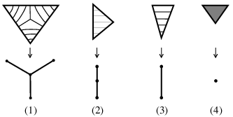
Refer to caption — Figure 1: A tight map of a simplex to a tree: (1) the vertices map to the endpoints of a triod; (2) the vertices map to three distinct points on an arc; (3) the vertices map to two points on an arc; (4) the vertices map to a single point.

A track pattern in a simplicial 2-complex $L$ is a 1-dimensional complex $P$ embedded in $L$ , such that for each 2-simplex $\sigma$ in $L$ , $P\cap\sigma$ is a disjoint union of finitely many arcs, each component of which connects points in the interiors of two distinct edges of $\sigma$ . For each edge $e$ of $L$ and each $x\in P\cap e$ , each 2-simplex $\sigma$ incident to $e$ therefore contains a component of $t\cap\sigma$ incident to $x$ . A track $t$ is a connected track pattern. Given a track pattern $P$ , a subset of $P$ is a track if and only if it is a component of $P$ . Two tracks $t,t^{\prime}$ are isotopic if there is an ambient isotopy of $L$ preserving each cell and taking $t$ to $t^{\prime}$ .

Suppose that $L$ is simply connected. Given a finite track $t$ in $L$ , the set $L-t$ has two components, and $t$ has a regular neighborhood which is a trivial $I$ -bundle over $t$ ; if each of the components of $L-t$ is unbounded then we say that $t$ is an essential track in $L$ . More generally, a finite track pattern $P$ in $L$ has finitely many components, and $P$ has an essential component if and only if there is an essential decomposition $L-P=U\cup V$ where $U,V$ are disjoint, nonempty, and unbounded, and each of $U,V$ is a union of components of $L-P$ . This fact is proved by induction on the number of components of $P$ : if $t$ is an inessential component of $P$ then the bounded component $W$ of $L-t$ can be conglomerated with whichever of $U$ or $V$ lies opposite $t$ from $W$ , showing that $L-(P-t)$ has an essential decomposition.

For example, if $f\colon L\to T$ is a tight map from a simplicial 2-complex to a tree, then for each $x\in T-T^{0}$ the set $f^{-1}(x)$ is a track pattern in $L$ ; see Figure 1. Moreover, if $x$ separates $T$ into two unbounded components, and if $f^{-1}(x)$ is finite, then $f^{-1}(x)$ has an essential component.

Theorem 5.7 (Tracks Theorem).

Let $H$ be a group, $L$ a simply connected simplicial $2$ -complex on which $H$ has a cocompact action, $T$ a simplicial tree with no valence $1$ vertices, and $\pi\colon L\to T$ a tight quasi-isometry. Suppose that $L$ is uniformly locally finite along edges, and that the tracks $\pi^{-1}(x)$ , $x\in T-T^{0}$ are uniformly finite. Then there is an $H$ -equivariant track pattern $P$ in $L$ such that the components of $P$ are finite and pairwise nonisotopic, and each component of $L-P$ is a bounded 2-complex (though not necessarily finite).

Note that conclusions (3) and (4) of Lemma 5.5 exactly match the finiteness conditions in the hypotheses of this theorem, so the theorem applies.

From the track pattern $P\subset L$ we construct a dual tree $T^{\prime}$ , with one vertex $v_{C}$ for each component $C$ of $L-P$ , and one edge $e_{t}$ for each track $t$ in $P$ . The action of $H$ on $L$ and $P$ induces an action on $T^{\prime}$ . There is an $H$ -equivariant map $L\to T^{\prime}$ defined as follows: for each track $t$ in $P$ the map $\pi^{\prime}\colon L\to T^{\prime}$ takes a regular neighborhood of $t$ to the corresponding edge $e_{t}$ ; for each component $C$ of $L-P$ the map $\pi^{\prime}$ takes $C$ minus the regular neighborhoods of incident tracks to the corresponding vertex $v_{C}$ .

We claim that the map $\pi^{\prime}\colon L\to T^{\prime}$ is a quasi-isometry. This immediately follows from the fact that the components of $P$ and of $L-P$ are bounded, and that there is a uniformly finite number of components of $P$ intersecting each edge of $L$ , which is a consequence of cocompactness of the $H$ -action on $L$ .

From the quasi-isometries $\pi^{\prime}\colon L\to T^{\prime}$ , $\pi\colon L\to T$ , the first $H$ -equivariant and the second $H$ -almost equivariant, we obtain an $H$ -almost equivariant quasi-isometry $T^{\prime}\to T$ . In Step 3 we shall move this quasi-isometry a bounded amount to obtain an explicit $H$ -almost equivariant quasi-isometry $\rho\colon\VE(T^{\prime})\to\VE(T)$ satisfying some important properties.

The action of $H$ on $T^{\prime}$ is cocompact. The action may have edge inversions; if so, subdivide each inverted edge at its barycenter to obtain an action without inversions. This subdivision does not change the commensurability classes of vertex and edge stabilizers. We may therefore assume that $H$ has no edge inversions, and so the quotient $T^{\prime}/H={\mathcal{G}}^{\prime}$ is a graph of groups with $H=\pi_{1}{\mathcal{G}}^{\prime}$ . Note that we have not yet been careful to insure irreducibility of ${\mathcal{G}}^{\prime}$ .

Let $X^{\prime}\to T^{\prime}$ be a tree of spaces for ${\mathcal{G}}^{\prime}$ . The group $H$ acts, properly discontinuously and cocompactly, on $X^{\prime}$ . As usual, the $H$ quasi-action on $X$ and the $H$ action on $X^{\prime}$ induce an $H$ -almost equivariant quasi-isometry $f\colon X\to X^{\prime}$ .

We now drop the simplicial triangulation $L$ , which was needed only to apply the Tracks Theorem 5.7, and revert to the original cell structure on $K$ . The ambient topological space and the set of locally infinite vertices is unchanged—indeed, every vertex of $K$ is locally infinite. The construction of the dual tree $T^{\prime}$ from the track pattern $P\subset K$ , which depends only on topology and not on cell structure, is also unchanged.

Step 3: Coarse respect of vertex and edge spaces.

It remains to make ${\mathcal{G}}^{\prime}$ irreducible, prove that the result has finite depth, and prove that $f\colon X\to X^{\prime}$ coarsely respects vertex and edge spaces. The main work is to analyze the subgroups of $H$ that stabilize the vertices and edges of $T^{\prime}$ , compare them to the subgroups stabilizing cells of $K$ , and use Corollary 5.6 to compare them with the vertex and edge spaces of $X$ .

We decompose $\VE(T^{\prime})={\mathcal{V}}(T^{\prime})\cup{\mathcal{E}}(T^{\prime})={\mathcal{V}}^{\infty}(T^{\prime})\cup{\mathcal{V}}^{\text{fin}}(T^{\prime})\cup{\mathcal{E}}(T^{\prime})$ , where ${\mathcal{V}}^{\infty}$ denotes vertices of infinite valence and ${\mathcal{V}}^{\text{fin}}$ denotes finite valence. We shall give a more explicit construction of the $H$ -almost equivariant quasi-isometry $\rho\colon\VE(T^{\prime})\to\VE(T)$ , as the union of a bijection ${\mathcal{V}}^{\infty}(T^{\prime})\to{\mathcal{V}}^{\infty}(T)$ a map ${\mathcal{V}}^{\text{fin}}(T^{\prime})\to{\mathcal{E}}(T)$ , and a map ${\mathcal{E}}(T^{\prime})\to{\mathcal{E}}(T)$ . It will be evident from this construction that $\rho$ agrees, within uniformly finite distance, with $\pi\circ\pi^{-1}$ . Moreover, we shall obtain (nonuniform) coarse equivalences

{\mathcal{O}}(\Stab(a))\stackrel{{\scriptstyle\scriptscriptstyle{c}}}{{=}}X_{\rho a}\quad\text{for all}\quad a\in\VE(T^{\prime})

Consider an infinite valence vertex $v_{C}\in{\mathcal{V}}^{\infty}(T^{\prime})$ . The corresponding component $C$ of $K-P$ has a frontier in $K$ consisting of infinitely many tracks. The only way this can happen is if $C$ contains at least one vertex of $K$ , because $K$ is uniformly locally finite along edges and $C$ is a bounded 2-complex. The question arises whether $C$ can contain more than one vertex of $K$ , and the answer is no:

Lemma 5.8.

Every component $C$ of $K-P$ contains at most one vertex of $K$ .

Proof.

We shall identify each vertex $v\in K$ with its image $\pi v\in{\mathcal{V}}^{\infty}(T)$ .

Suppose $C$ contains $2$ or more vertices $v_{0},v_{1}$ of $K$ .

We claim that $C$ contains an infinite sequence of vertices $v_{0},v_{1},v_{2},\ldots$ whose images under $\pi$ lie, in order, along some ray in the tree $T$ , diverging to the end of that ray. This contradicts the fact that the image of the bounded subset $C\subset K$ under the quasi-isometry $\pi\colon K\to T$ is a bounded subset of $T$ .

The claim is proved by induction. Suppose we have obtained a sequence $v_{0},\ldots,v_{k}$ of vertices of $K$ , each contained in $C$ , whose images under $\pi$ lie in order along a segment of $T$ . Let $e$ be the first edge of $T$ from $v_{k}$ to $v_{k-1}$ , and let $T_{e}$ be the component of $T-e$ containing $v_{k-1}$ . We shall show that $\Stab(v_{k})$ , a subgroup of $\Stab(C)$ , contains an element $h$ such that $h\cdot v_{k-1}\not\in T_{e}$ , for then $v_{k+1}=h\cdot v_{k-1}$ lies in $C$ and the sequence $v_{0},\ldots,v_{k+1}$ projects to a sequence in order along a segment of $T$ .

To construct the desired $h\in\Stab(v_{k})$ , note that the quasi-action of $\Stab(v_{k})$ on $T$ keeps $v_{k-1}$ within a bounded neighborhood of $v_{k}$ , and so there is a constant $A$ with the following properties for each $h\in\Stab(v_{k})$ :

•

The intersection $X_{v_{k}}\stackrel{{\scriptstyle\scriptscriptstyle{[A]}}}{{\cap}}X_{h\cdot v_{k-1}}$ realizes the coarse intersection of $X_{v_{k}}$ and $h\cdot X_{v_{k-1}}$ .
•

Letting $e_{h}$ denote the first edge of $T$ from $v_{k}$ to $h\cdot v_{k-1}$ , we have $X_{v_{k}}\stackrel{{\scriptstyle\scriptscriptstyle{[A]}}}{{\cap}}X_{h\cdot v_{k-1}}\stackrel{{\scriptstyle\scriptscriptstyle{[A]}}}{{\subset}}X_{e_{h}}$ .

But the quasi-action of $\Stab(v_{k})$ on $X_{v_{k}}$ is cobounded, and the coarse containment of $X_{e}$ in the vertex space $X_{v_{k}}$ is a strict coarse containment, and so there exists $h\in\Stab(v_{k})$ such that $X_{v_{k}}\stackrel{{\scriptstyle\scriptscriptstyle{[A]}}}{{\cap}}X_{h\cdot v_{k-1}}\not\stackrel{{\scriptstyle\scriptscriptstyle{[A]}}}{{\subset}}X_{e}$ , implying that $h\cdot v_{k-1}\not\in T_{e}$ . ∎

As a consequence of Lemma 5.8, the map $\pi^{\prime}\colon K\to T^{\prime}$ can be chosen to restrict to an $H$ -equivariant bijection between $K^{0}$ and ${\mathcal{V}}^{\infty}(T^{\prime})$ . Thus, $\pi^{\prime}{}^{-1}\circ\pi$ restricts to an $H$ -equivariant bijection between ${\mathcal{V}}^{\infty}(T^{\prime})$ and ${\mathcal{V}}^{\infty}(T)$ , which we take as the definition of the $\rho\bigm|{\mathcal{V}}^{\infty}(T^{\prime})$ . For each $v\in{\mathcal{V}}^{\infty}(T^{\prime})$ we clearly have $\Stab(v)=\Stab(\rho v)$ , and so ${\mathcal{O}}(\Stab(v))\stackrel{{\scriptstyle\scriptscriptstyle{c}}}{{=}}X_{\rho v}$ .

Now we turn to stabilizers of edges and of finite valence vertices of $T^{\prime}$ .

For any edge $e$ of $K$ , a subgroup $\Stab^{*}(e)<\Stab(e)$ of index at most two acts without inversion on $e$ , and so $\Stab^{*}(e)$ preserves each point of the finite set $P\cap e$ , each track of $P$ that intersects $e$ , each component of $e-P$ , and each component of $K-P$ that intersects $e$ .

We define $\rho\bigm|{\mathcal{V}}^{\text{fin}}(T^{\prime})$ , with values in ${\mathcal{E}}(T)$ , as follows. Consider a vertex $v_{C}\in{\mathcal{V}}^{\text{fin}}(T^{\prime})$ corresponding to a component $C$ of $K-P$ that contains no vertex of $K$ . We have $\Stab(v_{C})=\Stab(C)$ . The 2-complex $C$ is locally finite, and $C$ is bounded by Theorem 5.7, so $C$ is finite. Choose an edge $e^{\prime}$ of $K$ that intersects $C$ ; such an edge exists, for otherwise $C$ is contained in the interior of a 2-cell of $K$ and so $\partial C$ is an inessential track in $P$ , a contradiction. As noted above $\Stab^{*}(e^{\prime})$ preserves $C$ , and since there are only finitely many edges of $K$ intersecting $C$ it follows that $\Stab^{*}(e^{\prime})$ has finite index in $\Stab(C)=\Stab(v_{C})$ , and so $\Stab(e^{\prime})$ is commensurable to $\Stab(v_{C})$ . Choosing $e$ to be any edge of $T$ such that $f(e^{\prime})\supset e$ , we define $\rho(v_{C})=e$ . We have $\Stab(v_{C})\stackrel{{\scriptstyle\scriptscriptstyle{c}}}{{=}}\Stab(e^{\prime})$ , and so ${\mathcal{O}}(\Stab(v_{C}))\stackrel{{\scriptstyle\scriptscriptstyle{c}}}{{=}}{\mathcal{O}}(\Stab(e^{\prime}))\stackrel{{\scriptstyle\scriptscriptstyle{c}}}{{=}}X_{e}=X_{\rho(v_{C})}$ , where the second coarse equation follows from Corollary 5.6.

We define $\rho\bigm|{\mathcal{E}}(T^{\prime})$ , with values in ${\mathcal{E}}(T)$ , in a similar manner: for any edge $e_{t}$ of $T^{\prime}$ corresponding to a component $t$ of $P$ , choose an edge $e^{\prime}$ of $K$ that intersects $t$ , choose an edge $e$ of $T$ contained in $f(e^{\prime})$ , and define $\rho(e_{t})=e$ . The subgroups $\Stab(e_{t})$ and $\Stab(e)$ are commensurable, and as before using Corollary 5.6 we have $\Stab(e_{t})\stackrel{{\scriptstyle\scriptscriptstyle{c}}}{{=}}\Stab(\rho e_{t})$ and so ${\mathcal{O}}(\Stab(e_{t}))\stackrel{{\scriptstyle\scriptscriptstyle{c}}}{{=}}X_{\rho e_{t}}$ .

This completes the description of the quasi-isometry $\rho\colon\VE(T^{\prime})\to\VE(T)$ . For each $a\in\VE(T^{\prime})$ we have proved ${\mathcal{O}}(\Stab(a))\stackrel{{\scriptstyle\scriptscriptstyle{c}}}{{=}}X_{\rho a}$ . Also, for each $b\in\VE(T)$ there exists $a\in\VE(T^{\prime})$ such that $X_{b}\stackrel{{\scriptstyle\scriptscriptstyle{c}}}{{=}}X_{\rho a}$ . When $b\in{\mathcal{V}}^{\infty}(T)$ this follows from the fact that $\rho\colon{\mathcal{V}}^{\infty}(T^{\prime})\to{\mathcal{V}}^{\infty}(T)$ is a bijection. When $b$ is an edge this follows from the fact that the map $\pi\colon K\to T$ contains an edge $e$ such that $b\subset\pi(e)$ , and either $e$ intersects a component $t$ of $P$ corresponding to an edge $e_{t}\in{\mathcal{E}}(T^{\prime})$ and we take $a=e_{t}$ , or the endpoints of $e$ lie in some component $C$ of $K-P$ corresponding to a vertex $v_{C}\in{\mathcal{V}}^{\text{fin}}(T^{\prime})$ and we take $a=v_{C}$ .

We can now prove that ${\mathcal{G}}^{\prime}$ has depth one, as follows. The coarse inclusion lattice of vertex and edge spaces of $X^{\prime}$ is isomorphic to the coarse inclusion lattice of subgroups of $H$ stabilizing vertices and edges of $T^{\prime}$ , which as we have just shown is isomorphic to the coarse inclusion lattice of vertex and edge spaces of $X$ . Since the last lattice has depth one, so does the first lattice, and so ${\mathcal{G}}^{\prime}$ has depth one.

Also, the complete reduction process applied to ${\mathcal{G}}^{\prime}$ does not eliminate any coarse equivalence class of vertex and edge spaces, because every edge space in $X$ is the coarse intersection of two depth zero vertex spaces, and so the same is true in $X^{\prime}$ . Thus, we may assume that ${\mathcal{G}}^{\prime}$ is irreducible.

The last task is to prove that the quasi-isometry $f\colon X\to X^{\prime}$ coarsely respects vertex and edge spaces. We already know that the coarse inclusion lattices of vertex and edge spaces in $X$ and in $X^{\prime}$ are isomorphic, indeed the map $\rho\colon\VE(T^{\prime})\to\VE(T)$ provides the desired isomorphism, but we need to promote this to actual coarse respect with uniform constants, and our arguments so far have been rather sloppy about constants. But we can get around this problem as follows.

Knowing that ${\mathcal{G}}$ and ${\mathcal{G}}^{\prime}$ are irreducible, the Vertex–Edge Rigidity Theorem 2.11 applies, and it remains only to check that $f$ coarsely respects depth zero vertex spaces. We do this in the general setting of the Coboundedness Principle 2.5 as follows.

The set of depth zero vertex spaces of $X$ is a pattern in the sense of Section 2.3, and similarly for $X^{\prime}$ . Both of these patterns satisfy the local finiteness condition (a) and the coarse discreteness condition (b) of Section 2.3. The quasi-actions of $H$ on $X$ and on $X^{\prime}$ satisfy the coarse action condition (c) with respect to the patterns of depth zero vertex spaces. The action condition (d) is therefore also satisfied. We already have a bijection between the depth zero vertex spaces of $X$ and of $X^{\prime}$ , induced by the bijection $\rho\colon{\mathcal{V}}^{\infty}(T^{\prime})\to{\mathcal{V}}(T)$ , with the property that $\Stab(\rho(v^{\prime}))=\Stab(v^{\prime})$ for each $v^{\prime}\in{\mathcal{V}}^{\infty}(T^{\prime})$ . We are therefore reduced to proving the following:

Proposition 5.9.

Let $X,X^{\prime}$ be metric spaces, let ${\mathcal{A}},{\mathcal{A}}^{\prime}$ be patterns in $X,X^{\prime}$ satisfying the local finiteness condition (a), and let the group $H$ quasi-act properly and coboundedly on $X$ and on $X^{\prime}$ , satisfying the action condition (d) with respect to the patterns ${\mathcal{A}}$ and ${\mathcal{A}}^{\prime}$ . Let $f\colon X\to X^{\prime}$ be a quasi-isometry that is coarsely $H$ -equivariant, and suppose that there exists a bijection $f_{\#}\colon{\mathcal{A}}\to{\mathcal{A}}^{\prime}$ such that for each $A\in{\mathcal{A}}$ we have $\Stab(A)=\Stab(f_{\#}(A))$ . Then $f$ coarsely respects the patterns ${\mathcal{A}},{\mathcal{A}}^{\prime}$ , that is, for all $A\in{\mathcal{A}}$ we have $f(A)\stackrel{{\scriptstyle\scriptscriptstyle{[C]}}}{{=}}f_{\#}(A)$ , where the constant $C$ depends only on $X$ , $X^{\prime}$ , ${\mathcal{A}}$ , ${\mathcal{A}}^{\prime}$ , the quasi-isometry constants of $f$ , and the quasi-action constants of $H$ .

Proof.

Choose base points $p\in X$ , $p^{\prime}\in X^{\prime}$ . Consider $A\in{\mathcal{A}}$ and $A^{\prime}=f_{\#}(A)\in{\mathcal{A}}^{\prime}$ . The group $S=\Stab(A)=\Stab(A^{\prime})$ quasi-acts properly and coboundedly on $A$ and on $A^{\prime}$ , by the Coboundedness Principle 2.5, and it follows that $A\stackrel{{\scriptstyle\scriptscriptstyle{c}}}{{=}}S\cdot p$ and $A^{\prime}\stackrel{{\scriptstyle\scriptscriptstyle{c}}}{{=}}S\cdot p^{\prime}$ . Clearly $f(S\cdot p)\stackrel{{\scriptstyle\scriptscriptstyle{c}}}{{=}}S\cdot p^{\prime}$ , and putting it all together we see that $f(A)\stackrel{{\scriptstyle\scriptscriptstyle{c}}}{{=}}A^{\prime}$ .

We still need to establish uniformity of this coarse equivalence, that is, we need to show that $f(A)\stackrel{{\scriptstyle\scriptscriptstyle{[C]}}}{{=}}A^{\prime}$ where the constant $C$ is independent of $A\in{\mathcal{A}}$ . By the Coboundedness Principle 2.5, there are finitely many orbits of the action of $H$ on ${\mathcal{A}}$ and on ${\mathcal{A}}^{\prime}$ . Choosing a representative $A\in{\mathcal{A}}$ of each orbit and the corresponding orbit representative $A^{\prime}\in{\mathcal{A}}^{\prime}$ , we obtain a uniform constant $C$ over the choice of representatives. By the action condition (d), the quasi-action of $H$ on $X$ coarsely respects the pattern ${\mathcal{A}}$ , and the quasi-action on $X^{\prime}$ coarsely respects $A^{\prime}$ ; applying these quasi-actions, and enlarging $C$ as needed we obtain a uniform constant $C$ independent of $A\in{\mathcal{A}}$ . Moreover, if the orbit representatives of ${\mathcal{A}}$ are chosen to intersect a ball around $p$ whose size depends only on the quasi-action constants, and similarly for ${\mathcal{A}}^{\prime}$ , the required dependencies for the constant $C$ follow. ∎

This finishes the proof of Proposition 5.4, modulo more detailed proofs of Lemma 5.5 and the Tracks Theorem 5.7. ∎

5.4.1 Proof of Lemma 5.5: an action on a 2-complex.

We shall use the abbreviated terminology “raft of $T$ ” to mean a depth one raft of $T$ . This cannot cause confusion, because a depth zero raft of $T$ is the same thing as a fat vertex.

We first construct $K^{0}$ , then $K^{1}$ , and then $K^{2}$ , at each stage constructing the $H$ -action and the $H$ -almost equivariant quasi-isometry $\pi$ . Then we will establish the necessary finiteness properties.

The zero skeleton $K^{0}$ is identified with the set of fat vertices $V^{\infty}(T)$ . As is evident by now, there is a well-defined action of $H$ on the set of fat vertices of $T$ , characterized by $h\cdot X_{v}\stackrel{{\scriptstyle\scriptscriptstyle{c}}}{{=}}X_{h\cdot v}$ , and so we obtain the $H$ -action on $K^{0}$ and the $H$ -equivariant map $\pi\colon K^{0}\to V^{\infty}(T)$ . As usual, we will blur the distinction between $v\in K^{0}$ and $\pi v\in V^{\infty}(T)$ .

Since $G=\pi_{1}{\mathcal{G}}$ acts cocompactly on the tree $T$ , the set of fat vertices in $T$ is coarsely dense, meaning that each point of $T$ is a uniformly bounded distance from a fat vertex. As a consequence, there exists $R$ and $C$ such that, for any two fat vertices $u,v$ of $T$ , there is a sequence $u=x_{0},x_{1},\ldots,x_{n}=v$ of fat vertices for which $d(x_{i},x_{i+1})\leq R$ and with $n$ bounded by $C\,d(u,v)$ . If the geodesic segment from $x_{i}$ to $x_{i+1}$ contains any fat vertices, the sequence can be refined. Thus the following is natural:

Let $K^{1}_{\#}$ be the graph with vertex set the fat vertices of $T$ , and edges connecting pairs $\{u,v\}$ for which:

(i)

$d(u,v)\leq R$
(ii)

The geodesic segment in $T$ between $u$ and $v$ has no interior fat vertices (hereafter called a fat-free path).

The graph $K^{1}_{\#}$ has a canonical tight map $\pi\colon K^{1}_{\#}\to T$ , which by the above discussion is a quasi-isometry. By properties (i), (ii) above, $\pi(e)$ is contained in a raft of $T$ for each edge $e\subset K^{1}_{\#}$ , indeed more is true: there exists a constant $C$ such that:

(iii)

For any edge $e$ of $K^{1}_{\#}$ with endpoints $u,v\in K^{1}_{\#}$ , and for any edge $e^{\prime}$ in $\pi(e)$ , we have $(X_{u}\stackrel{{\scriptstyle\scriptscriptstyle{[C]}}}{{\cap}}X_{v})\stackrel{{\scriptstyle\scriptscriptstyle{[C]}}}{{=}}X_{e^{\prime}}$ .

While $H$ acts on the vertices of $K^{1}_{\#}$ , the action does not extend to the edges. We fix this as follows. Given two vertices $u,v$ of $K^{1}_{\#}$ , the property that $u,v$ are contained in the same raft of $T$ is $H$ -equivariant, and this property holds whenever $u,v$ are endpoints of an edge of $K^{1}_{\#}$ . If $u,v\in K^{0}$ are connected by an edge in $K^{1}_{\#}$ , if $h\in H$ , and if $h\cdot u$ , $h\cdot v$ are not connected by an edge in $K^{1}_{\#}$ , then connect them, and map this edge homeomorphically onto the unique path in $T$ connecting $\pi(h\cdot u)$ to $\pi(h\cdot v)$ ; as just explained, this path is contained in a raft of $T$ . We have now completed the construction of the 1-skeleton $K^{1}$ , of the $H$ action on $K^{1}$ , and of the $H$ -almost equivariant quasi-isometry $\pi\colon K^{1}\to T$ taking each edge of $K$ to a path contained in a single raft of $T$ .

For edges of $K^{1}$ , property (iii) above continues to hold with a larger value of $C$ , using the fact that the $H$ -quasi-action on $X$ respects fat vertex spaces. For each edge $e$ of $K^{1}$ let $X_{e}$ denote the union of the edge spaces $X_{e^{\prime}}$ over all $e^{\prime}\subset\pi e$ , and with $\partial e=\{u,v\}$ we have $(X_{u}\stackrel{{\scriptstyle\scriptscriptstyle{[C]}}}{{\cap}}X_{v})\stackrel{{\scriptstyle\scriptscriptstyle{[C]}}}{{=}}X_{e}$ and we also have $X_{e^{\prime}}\stackrel{{\scriptstyle\scriptscriptstyle{[2C]}}}{{=}}X_{e}$ .

An embedded loop in $K^{1}$ is minimal if any two points on the loop are connected by a segment of the loop which is geodesic in $K^{1}$ . To make $K^{1}$ simply connected we simply attach a 2-cell along every minimal loop. The resulting 2-complex is $K$ . The minimal loops are $H$ -equivariant and so $H$ acts on $K$ . Since $K^{1}$ is quasi-isometric to $T$ , there is an upper bound on the lengths of minimal loops. Also, the 2-cells do not change the quasi-isometry type, so the quasi-isometry $\pi\colon K^{1}\to T$ has an extension to an $H$ -almost equivariant quasi-isometry $K\to T$ , also denoted $\pi$ .

The next lemma plays a key role in establishing the finiteness properties of $K$ . Roughly speaking it says that the boundary of each 2-cell of $\sigma$ is mapped, via $\pi$ , into some raft of $T$ .

Lemma 5.10.

There is an $R\geq 0$ so that for every 2-cell $\sigma$ in $K_{0}$ and any edges $e_{1},e_{2}\subset\partial\sigma$ , we have $X_{e_{1}}\stackrel{{\scriptstyle\scriptscriptstyle{[R]}}}{{=}}X_{e_{2}}$ .

Proof.

Since $\partial\sigma$ has uniformly bounded length, to prove the lemma it suffices to find $T\geq 0$ so that if $e_{1},e_{2}$ are adjacent edges in $\partial\sigma$ then $X_{e_{1}}\stackrel{{\scriptstyle\scriptscriptstyle{[T]}}}{{=}}X_{e_{2}}$ . Let $v$ be the vertex of $K$ at which $e_{1},e_{2}$ meet.

Notice that if $e,e^{\prime}$ are edges of $K$ and if the paths $\pi e$ , $\pi e^{\prime}$ contain a common edge $e^{\prime\prime}$ of $T$ then $X_{e}\stackrel{{\scriptstyle\scriptscriptstyle{[2C]}}}{{=}}X_{e^{\prime\prime}}\stackrel{{\scriptstyle\scriptscriptstyle{[2C]}}}{{=}}X_{e^{\prime}}$ and so $X_{e}\stackrel{{\scriptstyle\scriptscriptstyle{[4C]}}}{{=}}X_{e^{\prime}}$ .

If the map $\pi$ folds $\partial\sigma$ at the vertex $v$ it follows that $\pi e_{1}$ , $\pi e_{2}$ contain a common edge of $T$ , and so $X_{e_{1}}\stackrel{{\scriptstyle\scriptscriptstyle{[4C]}}}{{=}}X_{e_{2}}$ .

Suppose that the map $\pi$ does not fold $\partial\sigma$ at the vertex $v$ . Let $w=\pi v$ and let $\pi^{-1}(w)\cap\partial\sigma=\{v\}\cup Y$ . Since the map $\pi$ is a bijection from vertices of $K$ to fat vertices of $T$ , each $y\in Y$ is an interior point of some edge $a_{y}$ of $\partial\sigma$ . Each of the paths $\pi(a_{y})$ determines an edge in the link of $w$ , each of the paths $\pi(e_{1})$ , $\pi(e_{2})$ determines a vertex in the link of $w$ , and the union of these vertices and edges is a connected subset of the link of $w$ , since $T$ is a tree. We can therefore find a sequence $e_{1}=a_{0},a_{1},\ldots,a_{M-1},a_{M}=e_{2}$ of edges in $\partial\sigma$ such that for $m=1,\ldots,M$ the paths $\pi(a_{m-1})$ and $\pi(a_{m})$ contain a common edge of $T$ , implying that $X_{a_{m-1}}\stackrel{{\scriptstyle\scriptscriptstyle{[4C]}}}{{=}}X_{a_{m}}$ . We therefore have $X_{e_{1}}\stackrel{{\scriptstyle\scriptscriptstyle{[4CM]}}}{{=}}X_{e_{2}}$ . Since $M$ is bounded by the length of $\partial\sigma$ we are done. ∎

Now we can prove the remaining contentions needed to establish Lemma 5.5:

Lemma 5.11.

The following properties hold:

1.

$K/H$ is finite.
2.

$K$ is uniformly locally finite along edges, that is, there is a uniform upper bound on the number of 2-cells whose boundary contains any fixed edge $e$ of $K$ .
3.

There is a uniform upper bound on the number of edges of $K$ whose image crosses any fixed edge of $T$ .

Proof.

Finiteness of vertices, edges, and faces of $K/H$ is an application of part (1) of the Coboundedness Principle 2.5 with appropriate patterns, as follows. In the case of vertices, we simply use the pattern of fat vertex spaces in $X$ . For edges, each edge $e$ of $K$ has a corresponding edge space $X_{e}$ , this pattern is locally finite, and for $h\in H$ we clearly have $h\cdot X_{e}\stackrel{{\scriptstyle\scriptscriptstyle{[R]}}}{{=}}X_{h\cdot e}$ for some uniform $R$ . For 2-cells, Lemma 5.10 shows that if we assign to each 2-cell $\sigma$ the pattern element $X_{\sigma}=\cup_{e\subset\sigma}X_{e}$ , then this pattern is locally finite and for $h\in H$ we have $h\cdot X_{\sigma}\stackrel{{\scriptstyle\scriptscriptstyle{[R]}}}{{=}}X_{h\cdot\sigma}$ for some uniform $R$ .

To prove that $K$ is uniformly locally finite along an edge $e$ , from Lemma 5.10 there is a constant $R$ such that if the boundary a 2-cell $\sigma$ contains $e$ then for any other edge $e^{\prime}\subset\partial\sigma$ we have $X_{e^{\prime}}\stackrel{{\scriptstyle\scriptscriptstyle{[R]}}}{{=}}X_{e}$ . Since the pattern of edge spaces is locally finite, there is a uniformly finite number of such edges $e^{\prime}$ . Since $\partial\sigma$ has uniformly bounded length and $\sigma$ is completely determined by its boundary, there is a uniformly finite number of such 2-cells $\sigma$ .

The proof of (3) is nearly identical to the proof of (2), using property (iii) for edges of $K$ in place of Lemma 5.10. ∎

This finishes the construction of $K$ and the proof of its properties, thus finishing Lemma 5.5.

5.4.2 Proof of the Tracks Theorem 5.7

Stallings discovered the principle that analogies with 3-manifold techniques could be applied to solve problems about general finitely generated groups [Sta68b]. An example of this principle is Dunwoody’s theory of tracks in 2-complexes [Dun85], which are analogous to Haken’s normal surfaces in a triangulated 3-manifolds [Hak61] — as it turns out, a normal surface intersects the 2-skeleton in a track, and the complexity of that track measures the complexity of the normal surface. Dunwoody [Dun85] used tracks to prove accessibility of finitely presented groups, an analogy to Haken’s theorem on boundedness of hierarchies of compact 3-manifolds.

Meanwhile, a completely different approach to 3-manifold theory was developed by Meeks and Yau [MY82], using minimal surfaces with respect to a Riemannian metric on the manifold to solve problems about 3-manifolds. Minimal surfaces and normal surfaces were combined by Jaco and Rubinstein [JR88] in their theory of PL minimal surfaces in 3-manifolds, resulting in a particularly elegant setting for 3-manifold theory. Casson’s Beijing notes on 3-manifolds [Cas] gave further simplifications in PL minimal surface theory, by using hyperbolic ideal triangles to impose a “hyperbolic structure” on the 2-skeleton minus the 0-skeleton.

The theme of our proof is that Casson’s approach to PL minimal surfaces, combined with Dunwoody’s tracks, can be used to solve problems about general groups acting on simply connected simplicial 2-complexes, even in contexts where the simplicial complex might not be locally finite. This theme was discovered independently by Niblo, who uses it to give a new proof of Stallings’ ends theorem [Nib04].

Recall the setting of the Tracks Theorem: a simply connected, simplicial 2-complex $L$ , a cocompact action of a group $H$ on $L$ , and a quasi-isometry $\pi\colon L\to T$ to a tree, so that $L$ is uniformly finite along edge interiors, and so that the tracks $\pi^{-1}(t)$ , for $t$ in the interior of an edge of $T$ , are uniformly finite.

In the course of the proof we will make use of the ends of $T$ and of $L$ . Ends cannot be defined in Freudenthal’s sense, using complementary components of compact sets, because $T$ and $L$ are not locally compact. Instead, we define ends in terms of complementary components of bounded subsets: the collection of bounded subsets forms a direct system under inclusion; the collection of unbounded complementary components of bounded subsets forms an inverse system under inclusion; and an end is defined to be an element of the inverse limit. This definition applies both in $T$ and in $L$ .

Alternatively, the tree $T$ with its simplicial metric is a Gromov hyperbolic space, the map $\pi\colon L\to T$ is a quasi-isometry and so $L$ is also Gromov hyperbolic, and $\pi$ induces a bijection of Gromov boundaries. For a simplicial complex quasi-isometric to a tree there is a bijection between the ends and the Gromov boundary. It follows that $\pi\colon L\to T$ induces a bijection of ends.

Now we follow Casson by imposing a “hyperbolic structure” on $L-L^{0}$ as follows. For each edge $e$ put a metric on $e-(\partial e)$ making it isometric to ${\mathbf{R}}$ . Choose a midpoint $\midpoint(e)\in e$ . For each 2-simplex $\sigma$ extend the metrics on the components of $(\partial\sigma)-\sigma^{0}$ to a metric on $\sigma-\sigma^{0}$ which is isometric to a hyperbolic ideal triangle, so that for each edge $e$ of $\sigma$ the point $\midpoint(e)$ matches the base of the perpendicular from the opposite ideal vertex. This matching condition guarantees that $L-L^{0}$ is a complete metric space. It also guarantees that any simplicial isomorphism of $L$ restricts to an isometry of $L-L^{0}$ .

For each track $\tau$ in $L$ , define the weight to be $w(\tau)=\left|\tau\cap L^{1}\right|$ , and define the length $\ell(\tau)$ to be the sum of the hyperbolic lengths of the components of $\tau$ intersected with each 2-simplex. Define the PL-length of $\tau$ to be the ordered pair $(w(\tau),\ell(\tau))\in{\mathbf{Z}}_{+}\times(0,\infty)$ . We compare PL-lengths using the dictionary ordering on ${\mathbf{Z}}_{+}\times(0,\infty)$ .

Consider an essential track $\tau$ in $L$ . We say that $\tau$ is weight minimal (called simply “minimal” in [Dun85]) if $w(\tau)$ is minimal among all essential tracks. We say that $\tau$ is PL-minimal if $(w(\tau),\ell(\tau))$ is minimal among all essential tracks in $L$ . We will need the fact that a weight minimal track intersects any 2-simplex in at most one arc ([Dun85], Proposition 3.1 and following comments).

Given a real number $\epsilon\in(0,1)$ , for any vertex $v$ there is a closed regular neighborhood $N^{\epsilon}(v)$ whose boundary link $\link^{\epsilon}(v)$ consists of a union of horocyclic segments of length $\epsilon$ in each 2-simplex incident to $v$ ; this follows from the matching condition. Moreover $N^{\epsilon}(v)\cap N^{\epsilon}(w)=\emptyset$ for $v\neq w$ ; this follows because in an ideal hyperbolic triangle, the three horocyclic segments of length $\epsilon$ about the three vertices are disjoint. A component of $\link^{\epsilon}(v)$ is called an $\epsilon$ -horocyclic track near $v$ ; we take the liberty of failing to mention either the $\epsilon$ or the $v$ . Note that an $\epsilon$ -horocyclic track is isotopic in $L-L^{0}$ to an $\epsilon^{\prime}$ -horocyclic track for any $\epsilon^{\prime}\leq\epsilon$ .

Lemma 5.12.

Suppose also that $L$ has an essential track. Then there exists an essential track $\tau\subset L$ which is either PL-minimal or horocyclic.

Proof.

Let $w_{\min}$ be the minimum of the positive integer $w(\tau)$ . Let $\tau_{i}$ be a sequence with $w(\tau_{i})=w_{\min}$ and with $\ell(\tau_{i})$ approaching the infimum. Since $H$ acts cocompactly on $L$ and isometrically on $L-L^{0}$ , after pulling back by appropriate elements of $H$ and passing to a finite subsequence we may assume that each $\tau_{i}$ intersects a certain edge $e$ . There are only finitely many isotopy classes of tracks with weight $w_{\min}$ that intersect $e$ , and so passing to a further subsequence we may assume that the isotopy class of $\tau_{i}$ is constant.

If any $\ell(\tau_{i})=0$ then we are done, for in that case $w(\tau_{i})=w_{\min}=1$ and $\tau_{i}$ is a point on an edge $e$ which does not bound any 2-simplex. So, we may assume that $\ell(\tau_{i})\neq 0$ .

Suppose there exists a vertex $v$ which is an accumulation point in $L$ of the sequence of tracks $\tau_{i}$ . Passing to a subsequence we may assume that $v=\lim x_{i}$ for some $x_{i}\in\tau_{i}$ . Since $v$ is infinitely far away from any point in $L-L^{0}$ with respect to the hyperbolic structure, and since $\ell(\tau_{i})$ is bounded, it follows that there is an $\epsilon>0$ such that $\tau_{i}\subset N^{\epsilon}(v)$ for sufficiently large $i$ . But now it is clear that $\tau_{i}$ is isotopic to a horocyclic track near $v$ .

Now suppose that no vertex is an accumulation point of the tracks $\tau_{i}$ . Since the isotopy class of $\tau_{i}$ in $L-L^{0}$ is fixed it follows that $\tau_{i}$ is contained in a bounded subset of $L-L^{0}$ , and so by the Ascoli-Arzela theorem $\tau_{i}$ converges to a track $\tau$ with $(w(\tau),\ell(\tau))$ minimized. ∎

Lemma 5.13.

There exists $\epsilon>0$ depending only on $L$ with the following property. Suppose that $\tau_{1},\tau_{2}$ are two essential tracks in $L$ , each of which is either PL-minimal or $\epsilon$ -horocyclic. Then either $\tau_{1}=\tau_{2}$ or $\tau_{1}\cap\tau_{2}=\emptyset$ .

Proof.

If no PL-minimal tracks exist then the lemma is obvious, with any $\epsilon\in(0,1)$ .

Suppose that PL-minimal tracks exist, and let $(w,\ell)$ be the least PL-length. If $\ell=0$ then the lemma is again obvious, so we assume $\ell>0$ .

Here’s how to choose $\epsilon$ . First pick an arbitrary number $\epsilon^{\prime}\in(0,1)$ . Now choose $\epsilon\in(0,\epsilon^{\prime})$ so that the distance from $\link^{\epsilon}(v)$ to $\link^{\epsilon^{\prime}}(v)$ is at least $\ell$ for any vertex $v$ ; $\epsilon=\epsilon^{\prime}e^{-\ell}$ will do nicely.

Given a vertex $v$ , clearly there are no PL-minimal tracks entirely contained in $N^{\epsilon^{\prime}}(v)$ , for any track in $N^{\epsilon^{\prime}}(v)$ may be shortened by isotoping towards $v$ . It follows that every PL-minimal track is disjoint from $N^{\epsilon}(v)$ . The lemma then follows as long as one or both of $\tau_{1},\tau_{2}$ are $\epsilon$ -horocyclic.

For the rest of the proof we may therefore assume that both $\tau_{1},\tau_{2}$ are PL-minimal. A simple variation argument (see [Cas]) shows that a PL-minimal track $\tau$ has the following “minimal surface” properties:

•

Each segment of intersection of $\tau$ with a 2-simplex is geodesic.
•

For oriented edge $e$ of $L$ , each point $x\in\tau\cap e$ , and each 2-simplex $\sigma$ of $L$ , letting $\theta(\tau,\sigma,x)$ be the angle between $\tau\cap\sigma$ and $e$ at the point $x$ , we have

$C(\tau,x)\equiv\sum_{\sigma}\cos\bigl(\theta(\tau,\sigma,x)\bigr)=0$

The fact that $C(\tau,x)=0$ can be seen by noting that $C(\tau,x)$ is the infinitesmal rate of change of $\ell(\tau)$ with respect to the position of $x$ on $e$ .

Suppose now that $\tau_{1}\cap\tau_{2}\neq\emptyset$ . We argue by contradiction, first in a special case and then in general.

Special Case:

$\tau_{1}$ and $\tau_{2}$ are in general position: $\tau_{1}\cap\tau_{2}$ consists of transverse intersection points in the interiors of 2-simplices. Following Dunwoody, let $J=L^{1}\cap(\tau_{1}\cup\tau_{2})$ , and noting that $\left|J\cap\partial\sigma\right|$ is even for each 2-simplex $\sigma$ , we obtain a finite track pattern $T_{J}$ , well-defined up to isotopy, satisfying $T_{J}\cap L^{1}=J$ .

Applying Proposition 3.2 of [Dun85], $T_{J}$ is a union of two essential, weight-minimal tracks, $T_{J}=\tau^{\prime}_{1}\cup\tau^{\prime}_{2}$ , and so $w(\tau^{\prime}_{i})=w(\tau_{i})=w$ , for $i=1,2$ .

Remark.

In [Dun85], a track was defined to be essential if each of its two complementary components has infinitely many vertices. In our present context, it is more appropriate to require the complementary components to be unbounded, and the proof of Dunwoody’s Proposition 3.2 is easily checked with that change.

Note that $T_{J}$ can be constructed in its isotopy class by doing a certain cut-and-paste on $\tau_{1}\cup\tau_{2}$ : for each 2-simplex $\sigma$ , and each $x\in\sigma\cap\tau_{1}\cap\tau_{2}$ , there are two choices for the cut-and-paste, but the choice is determined by the overall structure of $\sigma\cap\tau_{1}$ and $\sigma\cap\tau_{2}$ (see Figure 2). We thus have $T_{J}=\tau^{\prime}_{1}\cup\tau^{\prime}_{2}$ where

\ell(\tau^{\prime}_{1})+\ell(\tau^{\prime}_{2})=\ell(\tau_{1})+\ell(\tau_{2})=2\ell

and so there exists $i=1,2$ such that $\ell(\tau^{\prime}_{i})\leq\ell$ .

However, because of the assumption that $\tau_{1}\cap\tau_{2}$ is nonempty, say $x\in\sigma\cap\tau_{1}\cap\tau_{2}$ for some 2-simplex $\sigma$ , it follows that the cut-and-paste operation produces a corner of $\tau^{\prime}_{i}$ at $x$ with nonzero exterior angle. The length $\ell(\tau^{\prime}_{i})$ can therefore be shortened below the minimum length $\ell$ , a contradiction which shows that $\tau_{1}$ , $\tau_{2}$ cannot have a nonempty intersection in general position.

General Case:

$\tau_{1}$ and $\tau_{2}$ are not in general position. In particular, there is a point $x_{0}\in L^{1}\cap\tau_{1}\cap\tau_{2}$ such that $\tau_{1},\tau_{2}$ do not coincide in a neighborhood of $x$ . Since $C(\tau_{1},x_{0})=C(\tau_{2},x_{0})=0$ , it follows that there is a 2-simplex $\sigma$ incident to $x_{0}$ such that $\theta(\tau_{1},\sigma,x_{0})\neq\theta(\tau_{2},\sigma,x_{0})$ . Let $\phi_{0}=\left|\theta(\tau_{1},\sigma,x_{0})-\theta(\tau_{2},\sigma,x_{0})\right|$ , so $\phi_{0}>0$ .

Now we borrow Casson’s version of the “Meeks-Yau trick”: perturb $\tau_{1}$ and $\tau_{2}$ , raising their lengths by an arbitrarily tiny amount and making their cosine sums differ from zero by an arbitrarily tiny amount, to put $\tau_{1}$ and $\tau_{2}$ in general position. Do this in such a way as to make them intersect at a point $x$ in $\sigma$ near $x_{0}$ at an angle $\phi$ arbitrarily close to $\phi_{0}$ ; the tinier the perturbation, the closer $\phi$ will be to $\phi_{0}$ .

Now use the argument from the special case above, to produce two essential, weight minimal tracks $\tau^{\prime}_{1},\tau^{\prime}_{2}$ . The tracks $\tau^{\prime}_{1},\tau^{\prime}_{2}$ have corners at $x$ each with exterior angle $\phi$ , which is arbitrarily close to $\phi_{0}$ , and their cosine sums where they intersect $L^{1}$ are arbitrarily small. It follows that there is a $\delta>0$ , depending only on $\phi_{0}$ , so that by straightening $\tau^{\prime}_{1},\tau^{\prime}_{2}$ near $x$ the values of $\ell(\tau^{\prime}_{1})$ , $\ell(\tau^{\prime}_{2})$ can each be reduced by at least $\delta$ . However, the perturbation can be chosen so tiny that

\ell(\tau^{\prime}_{1})+\ell(\tau^{\prime}_{2})<\ell(\tau_{1})+\ell(\tau_{2})+\delta=2\ell+\delta

and therefore one of $\ell(\tau^{\prime}_{1}),\ell(\tau^{\prime}_{2})$ can be reduced below $\ell$ , a contradiction. ∎

Now we put the pieces together to prove the following:

Lemma 5.14 (Tracks exist).

Under the hypotheses of the Tracks Theorem, if $L$ is unbounded then there exists an $H$ -equivariant, essential, nonempty track pattern $P\subset L$ .

Proof.

Since $L$ is unbounded and $L,T$ are quasi-isometric, $T$ is also unbounded.

We use the coboundedness of the action of $H$ on $L$ to show that $L$ and $T$ have at least two ends. For a tree with a cococompact group action even more is true: the tree is either bounded, quasi-isometric to a line, or “bushy” meaning that the tree is quasi-isometric to a tree of constant valence $\geq 3$ . This was proved in [MSW03] for trees of uniformly bounded valence with the additional condition that the bushy tree of the conclusion has constant finite valence; but if one drops the hypothesis of uniformly bounded valence one need only weaken the conclusion to allow a bushy tree whose valence is a constant of unrestricted cardinality. The same proof works for a tree with a cobounded quasi-action, and we can apply that to our present situation since the cobounded action of $H$ on $L$ can be quasi-conjugated to give a cobounded quasi-action on $T$ .

For convenience here is a detailed proof, using the coboundedness of the action of $H$ on $L$ , that if $L$ is unbounded and quasi-isometric to a tree $T$ then $L$ has at least two ends.

A subset of a metric space if $r$ -deep if that subset contains an ambient metric ball of radius $r$ . Since the tree $T$ is unbounded, there is an infinite ray leaving every compact set, and so for each $r>0$ there exists an edge $e$ such that $T-e$ has at least two $r$ -deep components. Since $L$ and $T$ are quasi-isometric, it follows that there is a constant $k>0$ such that for each $s>0$ there exists a point $x$ such that $L-B(x,k)$ has at least two $s$ -deep components. Since $H$ acts coboundedly on $L$ , there exists $d>0$ such that for all $p,x\in L$ there exists $h\in H$ such that $d_{L}(p,h\cdot x)\leq d$ . This implies that, letting $l=k+d$ , for any $s>0$ and any point $p\in L$ the set $L-B(p,l)$ has at least two $s$ -deep components. Fix a point $p_{0}=q_{0}$ , fix $s>l$ , and let $C_{0},D_{0}$ be two $s$ -deep components of $L-B(p_{0},l)=L-B(q_{0},l)$ . We show that $C_{0},D_{0}$ are both unbounded. For $i\geq 1$ , inductively pick $p_{i}$ so that $B(p_{i},l)\subset B(p_{i},s)\subset C_{i-1}$ . There are at least two $s$ -deep components of $L-B(p_{i},l)$ , only one of which can contain $B(p_{i-1},l)$ , so pick $C_{i}$ to be a different one. Similarly, pick $q_{i}$ so that $B(q_{i},l)\subset B(q_{i},s)\subset D_{i-1}$ , and pick an $s$ -deep component $D_{i}$ of $L-B(q_{i},l)$ which does not contain $B(q_{i-1},l)$ . It follows that $p_{1},p_{2},p_{3},\ldots$ is a sequence of points in $C_{0}$ which gets arbitrarily far from $p_{0}$ , and $q_{1},q_{2},q_{3},\ldots$ is a sequence in $D_{0}$ which gets arbitrarily far from $q_{0}=p_{0}$ . This shows that $L$ has at least two ends. The tree $T$ , being quasi-isometric to $L$ , also has at least two ends.

Since $T$ has at least two ends, there is a point $t$ in the interior of some edge such that $T-t$ has two unbounded components, and it follows that the finite track pattern $\pi^{-1}(t)$ has an essential component. This shows that $L$ has a finite, essential track.

Applying Lemmas 5.12 and 5.13, it follows that $L$ has an essential track $\tau$ which is either PL-minimal or $\epsilon$ -horocyclic, where $\epsilon$ is chosen as in Lemma 5.13. Since $H$ acts on $L$ isometrically, it follows that $h(\tau)$ is PL-minimal or $\epsilon$ -horocyclic for each $h\in H$ . Therefore, for any $h,h^{\prime}\in H$ we apply Lemma 5.13 and conclude that either $h(\tau)=h^{\prime}(\tau)$ or $h(\tau)\cap h^{\prime}(\tau)=\emptyset$ . Thus, $P=H\cdot\tau$ is an $H$ -equivariant track pattern. ∎

Relative tracks.

We shall need a relative version of Lemma 5.14. A subcomplex $F\subset L^{1}$ is called peripheral if each component is compact and there is an open collar neighborhood $N_{F}$ equipped with a homeomorphism $(N_{F},F)\approx(F\times[0,1),F\times 0)$ .

Lemma 5.15 (Relative tracks exist).

Under the hypotheses of the Tracks Theorem, if $L$ is unbounded, and if $F$ is an $H$ -equivariant peripheral subcomplex of $L$ , then there exists an $H$ -equivariant, essential, nonempty track pattern $P\subset L$ such that $P\cap F=\emptyset$ .

Proof.

Given a track $\tau\subset L$ , we alter the definition of the weight $w(\tau)$ by assigning infinite weight to any point of $\tau\cap F$ , and so a track has finite weight if and only if it is disjoint from $F$ . Assuming that an essential track of finite weight exists, the proof of Lemma 5.14 goes through to show that there is a nonempty, $H$ -equivariant, essential track pattern $P$ whose components each have finite weight.

It remains to show that there exists an essential track in $L$ disjoint from $F$ .

We generalize the concept of a track pattern as follows: a pseudopattern is a 1-complex $P$ embedded in $L$ such that for each 2-simplex $\sigma$ of $L$ , each component of $\sigma\cap P$ is either a circle in the interior of $\sigma$ or a properly embedded arc with endpoints disjoint from the vertices of $\sigma$ ; any such arc with endpoints on the same edge of $\sigma$ is called a bight of $P$ . A pseudotrack is connected pseudopattern. The concept of essentiality is defined for a pseudotrack exactly as for a track. An essential pseudotrack is not a circle in the interior of any 2-simplex.

First we show that $L$ contains an essential pseudotrack disjoint from $F$ . By applying Lemma 5.14 we obtain an essential track $\tau$ in $L$ , but $L$ may intersect $F$ . Consider an essential decomposition $L-\tau=U\cup V$ . Let $F_{\tau}$ be the union of the components of $F$ that intersect $\tau$ , so $F_{\tau}$ is a finite 1-complex. Let $P^{\prime}$ be the pseudopattern obtained by using product structure on the collar neighborhood $N_{F}=F\times[0,1)$ to push $\tau\cup(F_{\tau}\cap U)$ into $L-F$ . To be precise, we assume that $\tau\cap N_{F}$ has the form $A\times[0,1)$ for some finite subset $A\subset F_{\tau}$ , and we take

P^{\prime}=\bigl(\tau-(A\times[0,1/2))\bigr)\cup\bigl((U\cap F_{\tau})\times 1/2\bigr)

There is an essential decomposition $L-P^{\prime}=U^{\prime}\cup V^{\prime}$ , where $V^{\prime}$ is the closure in $L-P^{\prime}$ of $V\cup\bigl((U\cap F_{\tau})\times[0,1/2)\bigr)$ , and where $U^{\prime}=(L-P^{\prime})-V^{\prime}$ . It follows, by the same argument for ordinary track patterns, that $P^{\prime}$ contains an essential pseudotrack $\tau^{\prime}$ . By construction, $\tau^{\prime}$ is disjoint from $F$ .

To go from an essential pseudotrack $\tau^{\prime}$ disjoint from $F$ to an essential track disjoint from $F$ , we inductively remove the bights, using a surgery procedure illustrated in Figure 3. To describe this procedure, consider an essential pseudotrack $\tau^{\prime}$ with essential decomposition $L-\tau^{\prime}=U^{\prime}\cup V^{\prime}$ . Let $b\subset\sigma$ be a bight of $\tau^{\prime}$ , with endpoints $x_{0},x_{1}$ on an edge $e$ of $L$ . We may choose $b$ to be innermost in $\sigma$ , so the segment $[x_{0},x_{1}]\subset e$ has interior disjoint from $\tau^{\prime}$ ; choose the notation so that the interior of $[x_{0},x_{1}]$ is contained in $V^{\prime}$ . Let $\sigma=\sigma_{0},\sigma_{1},\ldots,\sigma_{N}$ be the 2-simplices incident to $e$ . Let $s_{i}$ be a regular neighborhood of $x_{i}$ in $\tau^{\prime}$ , consisting of $N+1$ arcs sharing the common endpoint $x_{i}$ , with opposite endpoint $y_{in}$ in $\sigma_{n}$ . For $n=1,\ldots,N$ let $a_{n}$ be an arc in the interior of $\sigma_{n}$ with $a_{n}\cap\tau^{\prime}=\partial a_{n}=\{y_{0n},y_{1n}\}$ . The pseudopattern

P^{\prime\prime}=(\tau^{\prime}-(b\cup s_{0}\cup s_{1}))\cup a_{1}\cup\cdots\cup a_{N}

has strictly smaller weight than $\tau^{\prime}$ , and moreover $P^{\prime\prime}\cap L^{1}\subset\tau^{\prime}\cap L^{1}$ implying that $P^{\prime\prime}\cap F=\emptyset$ . There is an essential decomposition $L-P^{\prime\prime}=U^{\prime\prime}\cup V^{\prime\prime}$ described as follows: the connected pseudopattern $b\cup s_{0}\cup s_{1}\cup a_{1}\cup\cdots\cup a_{N}$ is inessential, with a bounded complementary component $W$ ; let $U^{\prime\prime}$ be the closure in $L-\tau^{\prime\prime}$ of $U^{\prime}\cup W$ , and let $V^{\prime\prime}=(L-\tau^{\prime\prime})-U^{\prime\prime}$ . It follows that $P^{\prime\prime}$ has a component $\tau^{\prime\prime}$ which is an essential pseudopattern disjoint from $F$ of smaller weight than $\tau^{\prime}$ , completing the induction. ∎

The Haken finiteness argument.

Consider a properly nesting sequence $P_{1}\subset\cdots\subset P_{K}$ of $H$ -equivariant, essential track patterns, such that no distinct components of $P_{K}$ are isotopic. We claim that there is a bound $K\leq K_{0}$ depending only on $L$ and $H$ . To see why, the quotient complex $L/H$ is finite, and so as noted in [Dun85] there exists $K_{0}$ such that any set of pairwise disjoint tracks in $L/H$ of cardinality $>K_{0}$ contains two tracks which are isotopic in $L/H$ . But if $P_{K}/H$ has a pair of isotopic components then $P_{K}$ has a pair of isotopic components. This shows that $K\leq K_{0}$ . It follows that there exists a sequence $P_{1}\subset\cdots\subset P_{K}$ as above which is maximal in the sense that it cannot be extended. Assuming maximality, to finish the Tracks Theorem we need to prove that the closure of every component of $L-P_{K}$ is a bounded 2-complex.

Boundedness.

Consider then a sequence $P_{1}\subset\cdots\subset P_{K}$ as above, and let $C$ be the closure of a component of $L-P_{K}$ . Assuming maximality of the sequence, we must show that $C$ is bounded.

Let $\Stab(C)$ denote the group of simplicial automorphisms of $L$ that stabilize $C$ . Noting that the quotient $C/\Stab(C)$ is the closure of a component of $L/H-P_{K}/H$ , it follows that $\Stab(C)$ acts cocompactly on $C$ .

Note that each component of the frontier $\Fr(C)$ of $C$ in $L$ is a component of $P_{K}$ ; we call these the frontier tracks of $C$ . The action of $\Stab(C)$ restricts to an action on the union of the frontier tracks of $C$ .

The cell structure on $C$ is described as follows. The 0-skeleton is $C\cap(L^{0}\cup P_{K}^{0})$ . The 1-skeleton is $C\cap(L^{1}\cup\cap P_{K})$ . Each 2-cell $c$ of $C$ is contained in a 2-simplex $\sigma$ of $L$ , $c$ is the closure of a component of $\sigma-P_{K}$ , and so $c$ is one of the following: $c=\sigma$ ; or $c$ is a quadrilateral with three sides in $\partial\sigma$ and one side in $\Fr(C)$ ; or $c$ is a pentagon with three sides in $\partial\sigma$ and two sides in $\Fr(C)$ ; or $c$ is a hexagon with three sides in $\partial\sigma$ and three sides in $\Fr(C)$ ; or $c$ is a quadrilateral with two sides in $\partial\sigma$ and two sides in $\Fr(C)$ ; or $c$ is a triangle with two sides in $\partial\sigma$ and one side in $\Fr(C)$ .

Next we prove that the inclusion $C\hookrightarrow L$ , which is clearly coarse Lipschitz, is actually a quasi-isometric embedding. Consider two vertices $x,y$ of $C$ connected by a geodesic path $\gamma$ in $L^{1}$ consisting of at most $m$ edges or half-edges of $L$ . Note that there are at most $m$ frontier tracks $\tau$ of $C$ such that $\gamma\cap A_{\tau}\neq\emptyset$ , because $A_{\tau}$ must contain a vertex of $\gamma$ . For each such $\tau$ , let $\gamma_{\tau}$ be the maximal subsegment of $\gamma$ such that $\partial\gamma_{\tau}\in A_{\tau}$ . Since the diameter of $\tau$ is uniformly bounded in $L$ , the segment $\gamma_{\tau}$ has uniformly bounded length. Choosing some order on the set of $\tau$ , inductively replace each $\gamma_{\tau}$ by an edge path in $\tau$ of uniformly bounded length. As each $\gamma_{\tau}$ is replaced, the identity of each subsequent $\gamma_{\tau^{\prime}}$ may change as one or both of its endpoints are eliminated by the previous replacement, but this change at worst decreases the length of $\gamma_{\tau^{\prime}}$ . It follows that $x,y$ are connected by a path in $C$ whose length is bounded by an affine function of the length of $\gamma$ , showing that $C\hookrightarrow L$ is a quasi-isometric embedding.

We may draw several conclusions from the fact that $C\hookrightarrow L$ is a quasi-isometric embedding. First, “boundedness” of $C$ is unambiguously defined: $C$ is a bounded 2-complex if and only if $C$ is a bounded subset of $L$ . Second, the map $\pi\colon C\to T$ induces an injection of ends, and so by restricting the range the map $\pi\colon C\to T_{C}$ induces a bijection of ends. Third, if $\tau$ is a track in $L$ which is contained in $C$ , is disjoint from $\Fr(C)$ , and is essential in $C$ , then $\tau$ is essential in $T$ and $\tau$ is not isotopic to any component of $P_{K}$ .

Assuming now that $C$ is not bounded, we prove that $P_{1}\subset\cdots\subset P_{K}$ is not maximal. The frontier $\Fr(C)$ is a $\Stab(C)$ -equivariant, peripheral subcomplex. Applying Lemma 5.15, $C$ has a $\Stab(C)$ -equivariant, essential track pattern $P_{C}$ disjoint from $\Fr(C)$ , and so disjoint from $P_{K}$ . Since the inclusion $C\hookrightarrow L$ is a quasi-isometry, each component of $P_{C}$ is essential in $L$ , and no component is isotopic to a comonent of $P_{K}$ . Acting on $P_{C}$ by the entire group $H$ , we obtain an $H$ -equivariant, essential track pattern $H\cdot P_{C}$ disjoint from $P_{K}$ and with no component isotopic to a component of $P_{K}$ . Letting $P_{K+1}=P_{K}\cup H\cdot P_{C}$ , it follows that $P_{1}\subset\cdot\subset P_{K}$ is not maximal.

There is a slight flaw in the above argument, because $C$ is not necessarily a simplicial complex. We can triangulate $C$ in a $\Stab(C)$ equivariant manner by putting a new vertex in the interior of any 2-cell $c$ that is not already a triangle, and coning off the boundary of $c$ . But now the problem is that $P_{C}$ , which is a track pattern with respect to the triangulation of $C$ , may only be a pseudopattern with respect to the original triangulation of $L$ . In the proof of Lemma 5.15, the key step is the production of an essential track $\tau$ in $C$ disjoint from $\Fr(C)$ , but $\tau$ may only be a pseudotrack with respect to the triangulation of $L$ ; however, any bights can be removed from $\tau$ by the same inductive process described in the proof of Lemma 5.15, and so we may indeed assume that $\tau$ and $P_{C}$ are true track patterns in $L$ .

This completes the proof of the Tracks Theorem.

5.5 Proof of the Tree Rigidity Theorem

Recall the setup of the theorem. ${\mathcal{G}}$ is a finite type, finite depth, irreducible graph of groups with Bass-Serre tree of spaces $X\to T$ . The finitely generated group $H$ quasi-acts properly and coboundedly on $X$ , and this quasi-action coarsely respects vertex and edge spaces, meaning that there is a quasi-action of $H$ on $\VE(T)$ and a constant $r\geq 0$ such that for each $h\in H$ and $a\in\VE(T)$ we have $h\cdot X_{a}\stackrel{{\scriptstyle\scriptscriptstyle{[r]}}}{{=}}X_{h\cdot a}$ , and for each $a^{\prime}\in\VE(T)$ there exists $a\in\VE(T)$ such that $X_{h\cdot a}\stackrel{{\scriptstyle\scriptscriptstyle{[r]}}}{{=}}X_{a^{\prime}}$ .

The depth of a vertex or edge space $X_{a}$ is determined by the position of $X_{a}$ in the coarse inclusion lattice of vertex or edge spaces: $X_{a}$ has depth zero if and only if $X_{a}$ is maximal in the coarse inclusion lattice; by induction, $X_{a}$ has depth $n$ if and only if $X_{a}$ does not have depth $<n$ and $X_{a}$ is maximal in the coarse inclusion lattice among vertex and edge spaces that do not have depth $<n$ . Since a quasi-isometry preserves coarse inclusions, it follows that $H$ preserves depth.

We must prove that there is a finite type, finite depth, irreducible graph of groups ${\mathcal{G}}^{\prime}$ with Bass-Serre tree of spaces $X^{\prime}\to T^{\prime}$ , and with fundamental group $\pi_{1}{\mathcal{G}}^{\prime}\approx H$ , so that the induced $H$ -almost equivariant quasi-isometry $X\to X^{\prime}$ coarsely respects vertex and edge spaces.

Two special cases have been proved: Proposition 5.3 handles the case where the edge spaces of $X$ are isolated, meaning that no two distinct edge spaces of $X$ are coarsely equivalent; and Proposition 5.4 handles the case when every edge space has depth one.

The induction argument for the general case is, in outline and in many details, the same as in Proposition 5.3. But the basis step in the general case will need the analysis of the homogeneous case carried out in [MSW03] (see Theorem 5.2), and the induction step will require Proposition 5.4.

Recall some notation and terminology. The tree $T$ is filtered by the subforests $F_{0}\subset F_{1}\subset\cdots\subset F_{N}=T$ , where $F_{n}$ consists of all vertices and edges of depth $\leq n$ . The components of $F_{n}$ are called the depth $n$ flotillas. For each subset ${\mathcal{A}}\subset\VE(T)$ we denote $X_{\mathcal{A}}=\cup_{a\in{\mathcal{A}}}X_{a}$ .

For each $n=0,\ldots,N$ consider the pattern in $X$ defined by

{\mathcal{P}}_{n}=\{X_{\mathcal{A}}\bigm|\text{${\mathcal{A}}$ is a depth $n$ flotilla.}\}

We wish to apply the Coboundedness Principle 2.5 to ${\mathcal{P}}_{n}$ , and so we must check the sufficient conditions (a–d) given in Section 2.3. Any bounded subset $B$ of $X$ intersects only finitely many edge or vertex spaces of $X$ , and since the depth $n$ flotillas are pairwise disjoint unions of vertex and edge spaces, it follows that $B$ intersects only finitely many of the elements of ${\mathcal{P}}_{n}$ ; in other words, ${\mathcal{P}}_{n}$ satisfies the Local Finiteness Condition (a) of Section 2.3. If ${\mathcal{A}}\neq{\mathcal{A}}^{\prime}$ are distinct depth $n$ flotillas then, as shown in the proof of the Vertex–Edge Rigidity Theorem 2.11, the coarse intersection $X_{\mathcal{A}}\stackrel{{\scriptstyle\scriptscriptstyle{c}}}{{\cap}}X_{{\mathcal{A}}^{\prime}}$ is coarsely contained in some edge space of depth $\geq n+1$ , and so $X_{\mathcal{A}}\not\stackrel{{\scriptstyle\scriptscriptstyle{c}}}{{=}}X_{{\mathcal{A}}^{\prime}}$ in $X$ ; this shows that ${\mathcal{P}}_{n}$ satisfies the Coarse Discreteness Condition (b). The proof of the Vertex–Edge Rigidity Theorem 2.11 also shows that a quasi-isometry that coarsely respects depth zero vertex and edge spaces will also coarsely respect flotillas of depth $n$ , and so the quasi-action of $H$ coarsely respects ${\mathcal{P}}_{n}$ , which is the Coarse Action Condition (c). It follows that there is an action of $H$ on the set of depth $n$ flotillas so that for each $h\in H$ and each depth $n$ flotilla ${\mathcal{A}}$ we have $h\cdot X_{\mathcal{A}}\stackrel{{\scriptstyle\scriptscriptstyle{[r]}}}{{=}}X_{h\cdot{\mathcal{A}}}$ , where $r\geq 0$ is independent of $h$ and ${\mathcal{A}}$ ; this is the Action Condition (d). The Coboundedness Principle 2.5 therefore applies, and so there are only finitely many $H$ -orbits of depth $n$ flotillas ${\mathcal{A}}$ , and the subgroup $\Stab({\mathcal{A}})=\Stab(X_{\mathcal{A}})$ quasi-acts properly and coboundedly on $X_{\mathcal{A}}$ . This quasi-action coarsely respects the vertex and edge spaces in $X_{\mathcal{A}}$ , because it is the restriction of the quasi-action of $H$ on $X$ —that is, there is an induced cobounded quasi-action of $\Stab({\mathcal{A}})$ on the tree ${\mathcal{A}}$ .

We now prove Tree Rigidity by induction. In the basis step, we replace $F_{0}$ by a forest $F^{\prime}_{0}$ on which $H$ acts. In the induction step, assuming we have replaced $F_{n}$ by a forest $F^{\prime}_{n}$ on which $H$ acts, we then replace $F_{n+1}$ by a forest $F^{\prime}_{n+1}$ on which $H$ acts. The replacements must always be realized by $H$ -almost equivariant quasi-isometries.

Consider a depth zero flotilla ${\mathcal{A}}$ of $T$ . By Proposition 2.6, ${\mathcal{A}}$ is either a point, a line, or a bushy tree with a Cantor set of ends. By the hypotheses of Tree Rigidity, ${\mathcal{A}}$ is not a line. When ${\mathcal{A}}$ is a point then we trivially have an action of $\Stab({\mathcal{A}})$ . Consider now the case where ${\mathcal{A}}$ is bushy, to which the results of [MSW03] apply. From Theorem 5.2 we may conclude that there is an action of $\Stab({\mathcal{A}})$ on a tree ${\mathcal{A}}^{\prime}$ , and a $\Stab({\mathcal{A}})$ -almost equivariant quasi-isometry ${\mathcal{A}}\to{\mathcal{A}}^{\prime}$ . But we need a little more: from Proposition 16 of [MSW03] the group $\Stab({\mathcal{A}})$ acts properly discontinuously and cocompactly on a Bass-Serre tree of spaces $X_{{\mathcal{A}}^{\prime}}\to{\mathcal{A}}^{\prime}$ with quotient graph of groups ${\mathcal{G}}_{{\mathcal{A}}^{\prime}}$ , and so we get an identification $\Stab({\mathcal{A}})\approx\pi_{1}{\mathcal{G}}_{{\mathcal{A}}^{\prime}}$ ; moreover, the induced $\Stab({\mathcal{A}})$ -almost equivariant quasi-isometry $X_{\mathcal{A}}\to X_{{\mathcal{A}}^{\prime}}$ coarsely respects vertex and edge spaces, inducing a $\Stab({\mathcal{A}})$ -almost equivariant quasi-isometry ${\mathcal{A}}\to{\mathcal{A}}^{\prime}$ .

In each $H$ -orbit of depth zero flotillas, pick a representative ${\mathcal{A}}_{0}$ , and apply the above argument to get a graph of groups ${\mathcal{G}}_{{\mathcal{A}}^{\prime}_{0}}$ with Bass-Serre tree of spaces $X_{{\mathcal{A}}^{\prime}_{0}}\to{\mathcal{A}}^{\prime}_{0}$ and an identification $\Stab({\mathcal{A}}_{0})\approx\pi_{1}{\mathcal{G}}_{{\mathcal{A}}^{\prime}_{0}}$ as above. We can now propogate the construction around by the action of $H$ , as follows. For each representative depth zero flotilla ${\mathcal{A}}_{0}$ and any flotilla ${\mathcal{A}}\neq{\mathcal{A}}_{0}$ in the orbit of ${\mathcal{A}}_{0}$ , choose $h\in H$ so that $h\cdot{\mathcal{A}}_{0}={\mathcal{A}}$ , and define $X_{{\mathcal{A}}^{\prime}}\to{\mathcal{A}}^{\prime}$ to be a disjoint copy of $X_{{\mathcal{A}}^{\prime}_{0}}\to{\mathcal{A}}^{\prime}_{0}$ with $\Stab({\mathcal{A}})=h\cdot\Stab({\mathcal{A}}_{0})\cdot h^{-1}$ acting properly discontinuously and cocompactly. The union of the trees ${\mathcal{A}}^{\prime}$ , over each depth zero flotilla ${\mathcal{A}}$ of $X$ , defines the forest $F^{\prime}_{0}$ . The union of the trees of spaces $X_{{\mathcal{A}}^{\prime}}$ defines the “forest of spaces” $X_{F^{\prime}_{0}}$ . The action of each group $\Stab({\mathcal{A}})$ , together with the maps $h\colon\Stab({\mathcal{A}}_{0})\to\Stab({\mathcal{A}})$ where $h\cdot{\mathcal{A}}_{0}={\mathcal{A}}$ , combine to give a well-defined action of $H$ on the forest of spaces $X_{F^{\prime}_{0}}\to F^{\prime}_{0}$ . For the moment we will not extend the metrics on the individual trees of spaces $X_{{\mathcal{A}}^{\prime}}$ to a metric on the forest of spaces $X_{F^{\prime}_{0}}$ , preferring instead to wait until the entire tree of spaces $X_{T^{\prime}}\to T^{\prime}$ has been constructed. This completes the basis step.

For the induction step, we assume that the forest of spaces $X_{F_{n-1}}\to F_{n-1}$ , on which $H$ quasiacts properly and coboundedly, coarsely respecting vertex and edge spaces, has been replaced by a forest of spaces $X_{F^{\prime}_{n-1}}\to F^{\prime}_{n-1}$ on which $H$ acts properly discontinuously and cocompactly, and there is an $H$ -almost equivariant map $f\colon X_{F_{n-1}}\to X_{F^{\prime}_{n-1}}$ which preserves the decomposition into trees of spaces, restricting to a quasi-isometry between corresponding trees of spaces that coarsely respects vertex and edge spaces within each tree of spaces; it follows that there is an induced $H$ -almost equivariant map $f_{\#}\colon F_{n-1}\to F^{\prime}_{n-1}$ which coarsely respects the decomposition into trees, restricting to a quasi-isometry between corresponding trees.

Consider a depth $n$ flotilla ${\mathcal{A}}$ , a component of $F_{n}$ . The group $\Stab({\mathcal{A}})$ quasi-acts properly and coboundedly on $X_{\mathcal{A}}$ , coarsely respecting the vertex and edge spaces in $X_{\mathcal{A}}$ . Let ${\mathcal{F}}=F_{n-1}\cap{\mathcal{A}}$ , the union of depth $n-1$ flotillas contained in ${\mathcal{A}}$ . We obtain a forest of spaces $X_{\mathcal{F}}\to{\mathcal{F}}$ . From the induction hypothesis, by restricting to ${\mathcal{A}}$ we obtain a forest of spaces $X_{{\mathcal{F}}^{\prime}}\to{\mathcal{F}}^{\prime}$ on which $\Stab({\mathcal{A}})$ acts properly discontinuously and cocompactly, and a $\Stab({\mathcal{A}})$ -almost equivariant map $f\colon X_{\mathcal{F}}\to X_{{\mathcal{F}}^{\prime}}$ , that respects the decomposition into trees of spaces, is a quasi-isometry on each tree of spaces, and that respects the vertex and edge spaces within each tree of spaces. There is an induced $\Stab({\mathcal{A}})$ -almost equivariant map $f_{\#}\colon{\mathcal{F}}\to{\mathcal{F}}^{\prime}$ that respects the decomposition into trees and is a quasi-isometry on each tree.

Our remaining goal is to construct a tree of spaces $X_{{\mathcal{A}}^{\prime}}\to{\mathcal{A}}^{\prime}$ on which $\Stab(A)$ acts properly discontinuously and cocompactly, and a $\Stab({\mathcal{A}})$ almost equivariant quasi-isometry $X_{\mathcal{A}}\to X_{{\mathcal{A}}^{\prime}}$ that coarsely respects vertex and edge spaces, descending to a $\Stab({\mathcal{A}})$ almost equivariant quasi-isometry ${\mathcal{A}}\to{\mathcal{A}}^{\prime}$ . Our construction will have the property that the depth $n-1$ subforest of ${\mathcal{A}}^{\prime}$ is $\Stab({\mathcal{A}})$ equivariantly identified with ${\mathcal{F}}^{\prime}$ , and that the restriction of $X_{{\mathcal{A}}^{\prime}}$ to ${\mathcal{F}}^{\prime}$ is equivariantly identified with $X_{{\mathcal{F}}^{\prime}}$ . This will complete the induction step, because we can carry this construction out for a representative of each orbit of the action of $H$ on the collection of deptn $n$ flotillas, and then propogate the construction around by $H$ -equivariance.

Consider the tree ${\mathcal{A}}/{\mathcal{F}}$ obtained by collapsing each component $F$ of ${\mathcal{F}}$ to a point that we shall denote $v_{F}$ . The composition $X_{{\mathcal{A}}/{\mathcal{F}}}=X_{\mathcal{A}}\to{\mathcal{A}}\to{\mathcal{A}}/{\mathcal{F}}$ defines a tree of spaces $X_{{\mathcal{A}}/{\mathcal{F}}}\to{\mathcal{A}}/{\mathcal{F}}$ with the property that every edge has depth one. Since the quasi-action of $\Stab(A)$ on $X_{\mathcal{A}}$ coarsely respects the spaces $X_{F}$ for each depth $n-1$ flotilla $F\subset{\mathcal{A}}$ , as well as the depth $n$ vertex and edge spaces in $X_{\mathcal{A}}$ , it follows that $\Stab(A)$ coarsely respects the depth zero vertex spaces $X_{v_{F}}$ of $X_{{\mathcal{A}}/{\mathcal{F}}}$ , as well as the depth one vertex and edge spaces of $X_{{\mathcal{A}}/{\mathcal{F}}}$ . We have now verified the hypotheses of Proposition 5.4, which is the special case of Tree Rigidity in which all edges have depth one. Applying that proposition, we obtain a tree of spaces that we shall denote $Y\to U$ , on which $\Stab(A)$ acts properly discontinuously and cocompactly, whose quotient graph of groups is finite type, of depth one, and irreducible, and we obtain a $\Stab(A)$ -almost equivariant quasi-isometry $f\colon X_{{\mathcal{A}}/{\mathcal{F}}}\to Y$ that coarsely respects vertex and edge spaces, descending to a quasi-isometry $f_{\#}\colon{\mathcal{A}}/{\mathcal{F}}\to U$ , so that $f(X_{a})\stackrel{{\scriptstyle\scriptscriptstyle{[C]}}}{{=}}Y_{f_{\#}(a)}$ for each edge or vertex $a$ of $X_{{\mathcal{A}}/{\mathcal{F}}}$ , where $C$ is a constant independent of $a$ ; we may also choose coarse inverses $\bar{f}\colon Y\to X_{{\mathcal{A}}/{\mathcal{F}}}$ and $\bar{f}_{\#}\colon U\to{\mathcal{A}}/{\mathcal{F}}$ with similar properties. Since the depth zero vertex spaces of $X_{{\mathcal{A}}/{\mathcal{F}}}$ are pairwise coarsely inequivalent, the same is true in $Y$ , and so $f_{\#}$ restricts to a bijection of depth zero vertices whose inverse is the restriction of $\bar{f}_{\#}$ .

Now we apply the techniques of Proposition 5.3, which is the special case of Tree Rigidity in which the edge spaces are isolated. Of course, in the present setting we do not have the isolation property for edge spaces of the tree of spaces $Y\to U$ . However, the isolation property for edge spaces was designed, somewhat artificially, for a particular purpose: so that the quasi-action strictly respects edge spaces, and hence descends to a true action on the Bass-Serre tree. In the present context, the action of the group $\Stab(A)$ on $Y$ does indeed strictly respect vertex and edge spaces, thereby descending to an action on the quotient tree $U$ .

Our goal now is the pretty much the same as in Proposition 5.3, and can be expressed in the present context as follows. Consider a depth zero vertex $v_{F}$ of ${\mathcal{A}}/{\mathcal{F}}$ corresponding to a component $F$ of ${\mathcal{F}}$ , let $v^{\prime}$ be the corresponding vertex of $U$ , and let $F^{\prime}$ be the corresponding component of ${\mathcal{F}}^{\prime}$ . We blow up the vertex $v^{\prime}$ , replacing it by the tree $F^{\prime}$ , and for each edge $e^{\prime}$ of $U$ incident to $v^{\prime}$ we must assign a vertex of $F^{\prime}$ to which $e^{\prime}$ should be attached. Let $\Stab^{*}(e^{\prime})$ be the subgroup of $\Stab(A)$ which fixes $e^{\prime}$ and preserves orientation on $e^{\prime}$ . Let $e=\bar{f}_{\#}(e^{\prime})$ , an edge of ${\mathcal{A}}/{\mathcal{F}}$ , and so we may also regard $e$ as an edge of ${\mathcal{A}}$ . Although we do not know whether $e$ has an endpoint in the tree $F$ , we do know that there is a vertex $w\in F$ which is uniformly close to $e$ in the tree $F$ , independent of the choice of $v_{F}$ and of $e^{\prime}$ . Since $\Stab^{*}(e^{\prime})$ fixes $e$ , it follows that, under the quasi-action of $\Stab(A)$ on $A$ , the $\Stab^{*}(e^{\prime})$ orbit of $e$ is uniformly bounded, independent of $v_{F}$ and of $e^{\prime}$ . This implies in turn that, under the quasi-action of $\Stab^{*}(e^{\prime})$ on $F$ , the orbit of $w$ is uniformly bounded, which implies further that, under the action of $\Stab^{*}(e^{\prime})$ on $F^{\prime}$ , the orbit of $f_{\#}(w)$ is uniformly bounded. Within the convex hull of this orbit there exists a point $w^{\prime}$ of $F^{\prime}$ that is fixed by the action of $\Stab^{*}(e^{\prime})$ . Subdividing $F^{\prime}$ at $w^{\prime}$ if necessary, we can attach $e^{\prime}$ to $w^{\prime}$ .

These attachments must be made in a $\Stab(A)$ -equivariant manner, and we do this by choosing a representative pair $(v^{\prime},e^{\prime})$ among the $\Stab(A)$ -orbits of adjacent pairs of vertices and edges of $U$ , assigning the attaching point for $e^{\prime}$ in $F^{\prime}$ , and then propogating this assignment around by the action of $\Stab(A)$ . This produces the desired tree ${\mathcal{A}}^{\prime}$ . The tree of spaces $X_{{\mathcal{A}}^{\prime}}$ has vertex and edge spaces of depth $\leq n-1$ taken from the vertex and edge spaces of $X_{F^{\prime}}$ , and $X_{{\mathcal{A}}^{\prime}}$ has vertex and edge spaces of depth $n$ taken from the depth one vertex and edge spaces of $Y$ . The attachments of edge spaces to vertex spaces may clearly be made in a $\Stab({\mathcal{A}})$ equivariant manner. Since $\Stab({\mathcal{A}})$ quasi-acts properly and coboundedly on $X_{\mathcal{A}}$ , and since it acts properly and coboundedly on $X_{{\mathcal{A}}^{\prime}}$ , we obtain a $\Stab({\mathcal{A}})$ almost equivariant quasi-isometry $X_{\mathcal{A}}\to X_{{\mathcal{A}}^{\prime}}$ which, by construction, coarsely respects vertex and edge spaces.

This completes the proof of the Tree Rigidity Theorem 2.12.

6 Main Theorems

With the machinery developed in the previous sections, we can now prove our main theorems.

Quasi-isometric rigidity.

Given a graph of groups ${\mathcal{G}}$ with Bass-Serre tree of spaces $X\to T$ , recall the main hypotheses:

(1)

${\mathcal{G}}$ is finite type, irreducible, and finite depth.
(2)

No depth zero raft of the Bass-Serre tree $T$ is a line.
(3)

Each depth zero vertex group is coarse $\PD$ .
(4)

The crossing graph condition holds for each depth zero vertex of $T$ which is a raft.
(5)

Each vertex and edge group of ${\mathcal{G}}$ is coarse finite type.

Theorem (1.5 Quasi-isometric rigidity theorem).

Proof.

Since $H$ is quasi-isometric to $\pi_{1}({\mathcal{G}})$ , it follows that $H$ quasi-acts properly and coboundedly on $X$ . By Theorems 2.10 and 2.11, this $H$ quasi-action coarsely respects the vertex and edge spaces. Thus we can apply Theorem 2.12 to get a graph of groups decomposition of $H$ with the desired properties. ∎

Quasi-isometric classification.

Given a group $G$ as above, Theorem 1.5 reduces the study of the quasi-isometry class of $G$ to studying groups which have splittings similar to that of $G$ . The content of Theorem 1.6 is that all such splittings of $H$ look coarsely the same as the splitting of $G$ :

Theorem (1.6 Quasi-isometric classification theorem).

Let ${\mathcal{G}},{\mathcal{G}}^{\prime}$ be graphs of groups satisfying (1)–(5) above. Let $X\to T$ , $X^{\prime}\to T^{\prime}$ be Bass-Serre trees of spaces for ${\mathcal{G}},{\mathcal{G}}^{\prime}$ , respectively. If $f\colon X\to X^{\prime}$ is a quasi-isometry then $f$ coarsely respects vertex and edge spaces. To be precise, for any $K\geq 1$ , $C\geq 0$ there exists $K^{\prime}\geq 1$ , $C^{\prime}\geq 0$ such that if $f\colon X\to X^{\prime}$ is a $K,C$ quasi-isometry then there exists a $K^{\prime},C^{\prime}$ quasi-isometry $f_{\#}\colon\VE(T)\to\VE(T^{\prime})$ such that the following hold:

•

If $a\in\VE(T)$ then $d_{\mathcal{H}}(f(X_{a}),X^{\prime}_{f_{\#}(a)})\leq C^{\prime}$ .
•

If $a^{\prime}\in\VE(T^{\prime})$ then there exists $a\in\VE(T)$ such that $d_{\mathcal{H}}(f(X_{a}),X^{\prime}_{a^{\prime}})\leq C^{\prime}$ .

Proof.

This is an immediate consequence of the Depth Zero Vertex Rigidity Theorem 2.10 and the Vertex–Edge Rigidity Theorem 2.11: the hypotheses of Theorem 2.10 hold, and so we conclude that $f$ coarsely respects depth zero vertex spaces; theorem 2.11 then applies to show that $f$ respects vertex and edge spaces of all depths as claimed. ∎

Graphs of coarse $\PD$ groups.

In many applications, Theorems 1.6 and 1.5 are combined: any group $H$ quasi-isometric to $\pi_{1}{\mathcal{G}}$ has a graph of groups decomposition ${\mathcal{G}}^{\prime}$ with properties similar to ${\mathcal{G}}$ ; and for any graph of groups decomposition ${\mathcal{G}}^{\prime}$ of $H$ with properties similar to ${\mathcal{G}}$ , any quasi-isometry $\pi_{1}{\mathcal{G}}\approx\pi_{1}{\mathcal{G}}^{\prime}\approx H$ coarsely respects vertex and edge spaces.

In most of our applications, the vertex and edge spaces are coarse $\PD$ spaces. Such graphs of groups are automatically finite depth, because an infinite index subgroup of a $\PD(n)$ groups has coarse dimension at most $n-1$ ; see Lemma 3.12.

Theorem (1.7 QI rigidity and classification for graphs of coarse $\PD$ groups).

Let ${\mathcal{G}}$ be a finite, irreducible graph of groups. Suppose that all vertex and edges groups of ${\mathcal{G}}$ are coarse Poincaré duality, no depth zero raft of the Bass-Serre tree $T$ is a line, and that the crossing graph of any one vertex depth zero raft of $T$ is either connected or empty. If $H$ is any finitely generated group quasi-isometric to $\pi_{1}{\mathcal{G}}$ then $H$ is the fundamental group of a finite type, irreducible graph of groups ${\mathcal{G}}^{\prime}$ , each of whose vertex groups and edge groups is coarse Poincaré duality, no depth zero raft of the Bass-Serre tree $T^{\prime}$ is a line, and the crossing graph of any one vertex depth zero raft is either connected or empty. Furthermore, any quasi-isometry $\pi_{1}{\mathcal{G}}\to\pi_{1}{\mathcal{G}}^{\prime}$ coarsely respects vertex and edge spaces.

Proof.

This follows immediately from Theorems 1.6 and 1.5 and the observation above that a graph of coarse $\PD$ groups is finite depth. ∎

It is also worth noting that for a graph of $\PD$ groups, the assumption that no depth zero raft is a line is essentially just a normalization condition for the splitting: any such raft can be “rolled-up” to a single vertex space to give a different splitting, and the new vertex group created in this way is a coarse $PD$ group of one dimension higher. Since the edges incident to this new vertex are the edges incident to the line raft in the old graph of groups, these edge spaces have codimension $\geq 2$ in the new vertex space, so the new vertex has empty crossing graph. The irreducibility condition is also a kind of normalization, as explained in Section 2.5: for any group $G$ , any finite depth graph of groups decomposition of $G$ can be converted into an irreducible one, and the resulting graph of groups is canonical in the sense that the commensurability lattice of vertex and edge stabilizers in the Bass-Serre tree is independent of the conversion process. Theorem 1.7 therefore applies to any finite graph of $\PD$ groups, subject to a translation of the crossing graph condition into a condition that is applied to each bounded depth zero raft of the Bass-Serre tree; making this translation is somewhat tedious, and so it is easier to state Theorem 1.7 in the normalized version above.

7 Applications and Examples

The general theorems of the previous section can be applied to a wide variety of graphs of groups. We give several specific examples, chosen with an eye towards applying additional rigidity tools to get even stronger conclusions. These stronger conclusions arise from considerations of “pattern rigidity” which we now discuss.

The idea behind pattern rigidity is that the conclusions of Theorems 1.6 and 1.5 contain more information than is immediately obvious. Given $G$ and $H$ as in the theorems, any quasi-isometry coarsely respects the $\VE$ lattice. Consider a depth zero vertex space $X_{v}$ for $G$ and the corresponding vertex space $X^{\prime}_{v^{\prime}}$ for $H$ . Not only does the quasi-isometry $G\to H$ restrict to give a quasi-isometry $X_{v}\to X^{\prime}_{v^{\prime}}$ , but this quasi-isometry respects the coarse intersections of $X_{v}$ and $X^{\prime}_{v^{\prime}}$ with other vertex spaces. This is often enough to prove that the quasi-isometry $X_{v}\to X^{\prime}_{v^{\prime}}$ induces an isomorphism between the pattern of edge spaces incident to $X_{v}$ and the pattern of edge spaces incident to $X^{\prime}_{v^{\prime}}$ . One then invokes one of several “pattern rigidity” theorems to reach even stronger conclusions about the quasi-isometry $X_{v}\to X^{\prime}_{v^{\prime}}$ .

First we discuss patterns in a very general context, before bringing in various pattern rigidity results.

7.1 Patterns of edge spaces in a vertex space.

Given a space $X$ , a pattern in $X$ is a collection $P$ of subsets of $X$ . If $P$ is a pattern in $X$ and $Q$ is a pattern in $Y$ , a quasi-isometry $\phi:X\to Y$ is said to respect the patterns $P$ and $Q$ if there is $C>0$ so that: for all $A\in P$ there exists $B\in Q$ for which

d_{\mathcal{H}}(\phi(A),B)<C

and likewise, for all $B\in Q$ there exists $A\in P$ for which

d_{\mathcal{H}}(\phi(A),B)<C

There are two important and closely related examples of concern to us: patterns of subgroup cosets in a group; and patterns of edge spaces in a vertex space.

Let $G$ be a finitely generated group and $H_{1},\cdots,H_{n}<G$ a finite collection of subgroups. The corresponding coset pattern $P$ is simply the collection of all left cosets of the $H_{i}$ . Let $X$ be a proper, geodesic metric space on which $G$ acts properly and coboundedly, let $Y_{1},\cdots,Y_{n}\subset X$ be subspaces such that $Y_{i}$ is invariant and cobounded under the action of the subgroup $H_{i}$ , and let $Q=\{g\cdot Y_{i}\bigm|g\in G,i=1,\ldots,n\}$ be the pattern of left translates. Any $G$ -equivariant quasi-isometry $G\mapsto X$ respects the patterns $P$ and $Q$ .

The situation above applies to graphs of groups as follows. Consider a finite type graph of groups ${\mathcal{G}}$ with Bass-Serre complex $X\to T$ , and let $p\colon T\to{\mathcal{G}}$ be the quotient map. Given a vertex $v\in T$ , let $Q$ be the pattern of incident edge spaces in $X_{v}$ , consisting of the images $Y_{e}$ of the attaching maps $X_{e}\to X_{v}$ , over all edges $e$ incident to $v$ . Alternatively, choosing edges $e_{1},\ldots,e_{n}$ representing the $\Stab(v)$ orbits of edges of $T$ incident to $v$ , $Q$ is just the left translate pattern of the subsets $Y_{e_{1}},\ldots,Y_{e_{n}}$ . If $e_{1},\ldots,e_{n}$ are chosen appropriately, the injections $\Stab(e_{1}),\ldots,\Stab(e_{n})\hookrightarrow\Stab(v)$ correspond via the isomorphism $\Stab(v)\to{\mathcal{G}}_{v}$ to the edge-to-vertex injections ${\mathcal{G}}_{p(e_{1})},\ldots,{\mathcal{G}}_{p(e_{n})}\hookrightarrow{\mathcal{G}}_{p(v)}$ , whose images define a coset pattern $Q$ in ${\mathcal{G}}_{p(v)}$ . It follows that any ${\mathcal{G}}_{p(v)}$ equivariant quasi-isometry ${\mathcal{G}}_{p(v)}\to X_{v}$ respects the patterns $P$ and $Q$ .

In many cases the group of quasi-isometries of a group preserving a coset pattern is quite small. As we will see in the next several sections, this phenomenon, called pattern rigidity, leads to very strong rigidity results for many classes of graphs of groups.

7.2 ${\mathbf{H}}^{n}$ vertex groups and ${\mathbf{Z}}$ edge groups.

The first example of a pattern rigidity theorem is the result of Schwartz ([Sch97]) on patterns of geodesics in ${\mathbf{H}}^{n}$ for $n\geq 3$ . Schwartz proves that if $M$ is a compact hyperbolic $n$ -manifold, $n\geq 3$ , and $c_{1},\cdots,c_{k}$ is any finite collection of closed geodesics in $M$ , and ${\mathcal{C}}$ is the pattern of geodesics in ${\mathbf{H}}^{n}$ covering the $c_{i}$ , then any quasi-isometry of ${\mathbf{H}}^{n}$ that coarsely preserves ${\mathcal{C}}$ is a bounded distance from an isometry that preserves ${\mathcal{C}}$ . It follows that the subgroup of $\QI({\mathbf{H}}^{n})$ that coarsely preserves ${\mathcal{C}}$ contains $\pi_{1}(M)$ as a subgroup of finite index.

Theorem 7.1.

Let ${\mathcal{G}}$ be a finite graph of groups whose vertex groups are fundamental groups of compact hyperbolic $n$ -manifolds, $n\geq 3$ , and whose edge groups are infinite cyclic. If $H$ is a finitely generated group quasi-isometric to $G=\pi_{1}({\mathcal{G}})$ then $H$ splits as a graph of groups whose depth zero vertex groups are commensurable to those of ${\mathcal{G}}$ and whose edge groups and positive depth vertex groups are virtually infinite cyclic.

Proof.

The vertex and edge spaces are coarse $\PD$ spaces, all depth zero rafts are one vertex rafts, and there are no codimension one edge-to-vertex inclusions. Thus theorem 1.7 applies to show that $H$ splits as a graph of groups ${\mathcal{G}}^{\prime}$ with depth zero vertex spaces quasi-isometric to ${\mathbf{H}}^{n}$ and edge groups quasi-isometric to ${\mathbf{Z}}$ .

By construction the quasi-isometry respects the vertex and edge spaces of this splitting, and thus the quasi-actions of the vertex groups on the vertex spaces of ${\mathcal{G}}$ preserve the patterns of edge spaces. Schwartz’ theorem [Sch97] thus shows that the depth zero vertex groups in the splitting ${\mathcal{G}}^{\prime}$ are commensurable to the corresponding groups in the splitting ${\mathcal{G}}$ . ∎

This means that to understand all groups quasi-isometric to $G$ , one only needs to study graphs of groups of the given type. One can read off many quasi-isometry invariants from the splittings. One simple example is:

Corollary 7.2.

Let $G_{i}=A_{i}*_{{\mathbf{Z}}}B_{i}$ for $i=1,2$ be amalgamated free products with $A_{i},B_{i}$ fundamental groups of closed hyperbolic manifolds of dimension $\geq 3$ , with ${\mathbf{Z}}$ including into $A_{i}$ and $B_{i}$ as maximal cyclic subgroups. If $G_{1}$ and $G_{2}$ are quasi-isometric then up to reordering, $A_{1}$ is commensurable to $A_{2}$ and $B_{1}$ is commensurable to $B_{2}$ . Further, these commensurators must respect, up to finite index, the cyclic subgroups. Thus, in particular, for fixed $A$ and $B$ there are infinitely many quasi-isometry classes of groups of the form $A*_{{\mathbf{Z}}}B$ .

Proof.

The Classification Theorem shows that any quasi-isometry between $G_{1}$ and $G_{2}$ coarsely respects the given splittings. The commensurability statements then follow from the same argument as in the proof of Theorem 7.1.

To see the infinitude of quasi-isometry types, one needs to check that the fundamental group of any compact hyperbolic $n$ -manifold contains infinitely many cyclic subgroups not commensurable to each other. This follows as any such manifold has infinitely many distinct primitive closed geodesics. ∎

A variation: ${\mathbf{H}}^{n}$ vertex groups and free edge groups.

The proof of Theorem 7.1 suggests other classes of groups to investigate. For example, consider an amalgamated free product $G_{1}*_{F}G_{2}$ where $G_{1},G_{2}$ are fundamental groups of closed hyperbolic manifolds of dimension $\geq 3$ , and $F$ is a finite rank free group including into each of $G_{1}$ and $G_{2}$ as a malnormal subgroup. The finite depth property follows from the malnormality hypothesis, and so our main QI-rigidity and classification theorems apply to this group. It follows that if the finitely generated group $H$ is quasi-isometric to $G_{1}*_{F}G_{2}$ then $H=\pi_{1}{\mathcal{G}}$ where ${\mathcal{G}}$ is a finite graph of groups whose vertex groups are quasi-isometric to either $G_{1}$ or $G_{2}$ and whose edge groups are quasi-isometric to $F$ . The edge groups are therefore virtually free, and each vertex group has a finite normal subgroup so that the quotient is a cocompact lattice in the isometries of hyperbolic space of some dimension. However, in this situation we do not know of any pattern rigidity result which would imply that the vertex groups of ${\mathcal{G}}$ are commensurable to $G_{1}$ or $G_{2}$ .

This invites some questions: Is there a pattern rigidity theorem for a free subgroup $F$ of a cocompact lattice $G$ acting on hyperbolic space? What if $F$ is quasiconvex? What if $F$ is quasiconvex and malnormal? In the latter situation, the limit sets of all conjugates of $F$ in $G$ would form a pairwise disjoint pattern of Cantor sets in the boundary of hyperbolic space, which might be an interesting starting point for pondering a generalization of Schwartz’ pattern rigidity theorem [Sch97].

7.3 ${\mathbf{H}}^{3}$ vertex groups and surface fiber edge groups.

In any context in which one has a pattern rigidity result analogous to the theorem of Schwartz used above, one can substantially strengthen the general results of Theorems 1.5 and 1.6. Here is a pattern rigidity result of Farb and Mosher for fibered hyperbolic 3-manifolds; the proof of this result ultimately depends on Schwartz’ result [Sch97].

Theorem 7.3 ([FM02b]).

Let $M$ be a hyperbolic $3$ -manifold which fibers over the circle with fiber $F$ . The subgroup of $\QI({\mathbf{H}}^{3})$ which coarsely preserves the pattern of cosets of $\pi_{1}(F)$ is a subgroup ${\mathcal{G}}$ of $\Isom({\mathbf{H}}^{3})$ which contains $\pi_{1}(M)$ as a finite index subgroup.

We can use this to prove a rigidity theorem for graphs of groups. Given a closed hyperbolic 3-manifold $M$ , a fiber subgroup of $\pi_{1}(M)$ is the image of an injection $\pi_{1}(F)\hookrightarrow\pi_{1}(M)$ where $M$ fibers over $S^{1}$ with fiber $F$ .

Theorem 7.4.

Let ${\mathcal{G}}$ be a finite graph of groups in which every vertex group is the fundamental group of a closed hyperbolic $3$ -manifold, every edge group is a surface group, and the image of every edge-to-vertex injection is a fiber subgroup. If $H$ is any finitely generated group quasi-isometric to $\pi_{1}({\mathcal{G}})$ then $H$ splits as a graph of groups whose depth zero vertex groups are commensurable to those of ${\mathcal{G}}$ , and whose edge groups are positive depth vertex groups are commensurable to surface groups.

Proof.

The case where ${\mathcal{G}}$ has no edges was proved by Gromov and Sullivan; see [CC92]. We may therefore assume ${\mathcal{G}}$ has at least one edge.

We modify the graph of groups ${\mathcal{G}}$ as follows. Suppose that $v$ is a vertex such that all the incident edge groups are contained in the same fiber subgroup $\pi_{1}(F)\hookrightarrow\pi_{1}(M)\approx{\mathcal{G}}_{v}$ . Blow up the vertex $v$ , replacing it by a vertex $v^{\prime}$ with group ${\mathcal{G}}_{v^{\prime}}\approx\pi_{1}(F)$ and an edge group $\pi_{1}(F)$ glued at both ends to ${\mathcal{G}}_{v^{\prime}}$ , thereby describing $\pi_{1}(M)$ as an HNN amalgamation with $\pi_{1}(F)$ as fiber. Call the resulting graph of groups ${\mathcal{G}}^{\prime}$ . This is a graph of $\PD$ groups, and as ${\mathcal{G}}$ has at least one edge, ${\mathcal{G}}^{\prime}$ has no line-like rafts. To apply Theorem 1.7 we need to check the crossing graph condition. If all vertex groups of ${\mathcal{G}}^{\prime}$ are surface groups then all crossing graphs are empty. Those vertices which are not surfaces are hyperbolic $3$ -manifold groups with at least two distinct fiber subgroups containing edge groups with finite index.

Claim 7.5.

If $M$ is a closed hyperbolic $3$ -manifold which fibers over the circle in two homotopically distinct ways, with fibers $F$ and $F^{\prime}$ , then every coset of $\pi_{1}(F)$ crosses every coset of $\pi_{1}(F^{\prime})$ .

Since $\pi_{1}(F)$ and $\pi_{1}(F^{\prime})$ are normal subgroups, all the cosets of each are parallel, so we only need to check that $\pi_{1}(F)$ crosses $\pi_{1}(F^{\prime})$ . This is immediate as a subset of $\pi_{1}(M)$ which stays to one side of $\pi_{1}(F)$ is contained in a half ray in $\pi_{1}(M)/\pi_{1}(F)\equiv{\mathbf{Z}}$ . For a subgroup, this means the image must be trivial, in other words, that the subgroups of $\pi_{1}(M)$ which do not cross $\pi_{1}(F)$ are the subgroups of $\pi_{1}(F)$ . Since $F$ and $F^{\prime}$ are non parallel fibers, they cross, proving the claim.

We can now apply Theorem 1.7 to produce the desired splitting of $H$ . The statement about commensurability types of depth zero vertex groups follows from Theorem 7.3, just as the similar statement in Theorem 7.1 followed from Schwartz’ pattern rigidity. This finishes the proof of Theorem 7.4. ∎

The Classification Theorem together with pattern rigidity and Theorem 7.3 can be used to give many quasi-isometry invariants of such groups, as in corollary 7.2. Here is one example:

Corollary 7.6.

Let $M_{i}$ , $i=1,2$ , be closed hyperbolic $3$ -manifolds each of which which fibers over the circle in two distinct ways, with fibers $F_{i}$ and $F^{\prime}_{i}$ . Let $T_{i}$ be an isomophism between a finite index subgroup of $\pi_{1}(F_{i})$ and $\pi_{1}(F^{\prime}_{i})$ , and let $G_{i}$ be the $HNN$ extension of $\pi_{1}(M_{i})$ over $T_{i}$ . If $G_{1}$ and $G_{2}$ are quasi-isometric then there is an isomorphism between finite index subgroups of $\pi_{1}(M_{1})$ and $\pi_{1}(M_{2})$ which (up to re-ordering) also commensurates $\pi_{1}(F_{1})$ with $\pi_{1}(F_{2})$ and $\pi_{1}(F^{\prime}_{1})$ with $\pi_{1}(F^{\prime}_{2})$ .

7.4 Surface vertex groups and cyclic edge groups.

For surfaces, connected crossing graph has a geometric interpretation. Consider first a closed hyperbolic surface $\Sigma$ and a collection of nontrivial conjugacy classes $c_{1},\ldots,c_{k}$ in $\pi_{1}\Sigma$ . These classes are represented by simple closed geodesics in $\Sigma$ , also denoted $c_{1},\ldots,c_{k}$ . We say that $c_{1},\ldots,c_{k}$ fill $\Sigma$ if the components of $\Sigma-(c_{1}\cup\cdots\cup c_{k})$ are all open discs. More generally, suppose that $\Sigma$ is a closed hyperbolic 2-orbifold, and $c_{1},\ldots,c_{k}$ are infinite order conjugacy classes in $\pi_{1}\Sigma$ . Each conjugacy class $c_{i}$ is still represented by a closed geodesic in $\Sigma$ , properly interpreted: $c_{i}$ can reflect across a mirror edge of the orbifold; and $c_{i}$ can pass through a cone point or a corner reflector. We say that $c_{1},\ldots,c_{k}$ fill $\Sigma$ if each component of $\Sigma-(c_{1}\cup\cdots\cup c_{k})$ is a 2-orbifold with finite fundamental group. In both cases, $c_{1},\ldots,c_{k}$ fill $\Sigma$ if and only if the union of the total lifts of $c_{1},\ldots,c_{k}$ to ${\mathbf{H}}^{2}$ has all of its complementary components being open discs with compact closure.

Lemma 7.7.

Let $\Sigma$ be a closed hyperbolic $2$ -orbifold, $G=\pi_{1}(\Sigma)$ . Let $c_{1},\cdots,c_{k}$ be a collection of non-trivial isotopy classes of closed geodesics on $\Sigma$ , and let $H_{i}$ be an infinite cyclic subgroup generated by an element of $G$ in the conjugacy class determined by $c_{i}$ . The crossing graph of the collection of conjugates of the $H_{i}$ in $G$ is connected if and only if the curves $c_{i}$ fill $\Sigma$ .

Proof.

Let $C$ be the collection of geodesics in ${\mathbf{H}}^{2}$ overing the $c_{i}$ . Note that $C$ is in one-to-one correspondence with the collection of subgroups of $G$ conjugate to the $H_{i}$ . Further, two such subgroups cross in the sense of section 3.1 if and only if the corresponding geodesics intersect in ${\mathbf{H}}^{2}$ . Thus the crossing graph is connected if and only if, $Z$ , the union of geodesics in $C$ , is a connected subset of ${\mathbf{H}}^{2}$ . The lemma therefore says that $Z$ is connected if and only if the complementary components of $Z$ are bounded.

Suppose $Z$ is connected. Let $U$ be a component of ${\mathbf{H}}^{2}-Z$ . Since the collection $C$ is locally finite, the stabilizer of $U$ in $G$ acts coboundedly on $U$ . If $U$ is unbounded this implies there is a non-trivial element of $G$ preserving $U$ , and hence, as $U$ is convex, $U$ conatains the axis of an element of $G$ . This axis is disjoint from all elements of $C$ and disconnects ${\mathbf{H}}^{2}$ . Since $Z$ is connected it must lie on one side of this axis. This is a contradiction as $Z$ is $G$ invariant and $G$ is cocompact on ${\mathbf{H}}^{2}$ . Thus all complementary components are bounded.

Next, suppose all components of ${\mathbf{H}}^{2}-Z$ are bounded. If $Z$ is not connected then there must be a component $U$ of this complement which borders two components of $Z$ . However, since $U$ is disk, its boundary is connected, which is a contradiction. ∎

Schwartz’s pattern rigidity result does not hold in general for patterns of geodesics on hyperbolic surfaces. However, Kapovich and Kleiner show that pattern rigidity does hold when the geodesics $c_{1},\cdots,c_{k}$ fill the surface; see [KK00] Lemma 22. This is equivalent to our assumption on crossing graphs, and so we have:

Theorem 7.8.

Let ${\mathcal{G}}$ be a graph of groups where every vertex group is the fundamental group of a closed hyperbolic $2$ -orbifold, and whose edge groups are virtual infinite cyclic groups. Assume that the edge groups at each vertex correspond to curves which fill. If $H$ is any finitely generated group quasi-isometric to $G=\pi_{1}({\mathcal{G}})$ then $H$ has a splitting with virtual surface groups as depth zero vertex groups and virtually cyclic positive depth vertex groups and edge groups. Further, the quasi-isometry $G\to H$ restricts to a commensurator on each vertex group.

Since all cocompact lattices in $SL_{2}({\mathbf{R}})$ are (abstractly) commensurable, one must look more closely at the consequences of the Classification Theorem to see that the graphs of groups in Theorem 7.8 are not all quasi-isometric. The key point is that it is certainly not true that any two finite collections of filling curves is commensurable to any other.

For explicit examples, let $T_{r}$ denote the reflection group of the hyperbolic triangle with angles $\pi/2$ , $\pi/4$ , $\pi/r$ . This has an index $2r$ subgroup which is the reflection group in a regular, right angled, hyperbolic polygon with $r$ sides. Consider the tiling of ${\mathbf{H}}^{2}$ by copies of this polygon, moved around by the group $T_{r}$ . Each side of each tile extends to a bi-infinite geodesic which is contained in the union of sides of the tiles. This pattern of geodesics, denoted ${\mathcal{S}}_{r}$ , is invariant under $T_{r}$ . Picking one geodesic in ${\mathcal{S}}_{r}$ , the subgroup of $T_{r}$ that stabilizes this geodesic is an infinite dihedral group denoted $D_{r}$ .

Consider the free product with amalgamations $T_{r}*_{D_{\infty}}T_{s}$ where $D_{\infty}$ includes to the subgroups $D_{r}\subset T_{r}$ and $D_{s}\subset T_{s}$ . We claim that the set of integers $\{r,s\}$ is a quasi-isometry invariant, thus giving infinitely many distinct quasi-isometry classes. To prove this it suffices to show that if $r\neq r^{\prime}$ then there is no quasi-isometry of ${\mathbf{H}}^{2}$ taking the pattern ${\mathcal{S}}_{r}$ to the pattern ${\mathcal{S}}_{r^{\prime}}$ . However, any such quasi-isometry takes two crossing geodesics in ${\mathcal{S}}_{r}$ to two crossing geodesics in ${\mathcal{S}}_{r^{\prime}}$ , and when $r\neq r^{\prime}$ there is clearly no bijection between ${\mathcal{S}}_{r}$ and ${\mathcal{S}}_{r^{\prime}}$ that preserves the relation of crossing.

7.5 Graphs of abelian groups.

For ${\mathbf{Z}}^{n}$ vertex groups, the crossing graph condition is simple: a subgroup $A<{\mathbf{Z}}^{n}$ crosses a subgroup $B\approx{\mathbf{Z}}^{n-1}$ if and only if $A$ is not virtually contained in $B$ , if and only if $A,B$ generate a finite index subgroup of ${\mathbf{Z}}^{n}$ .

The following generalized version of Theorem 1.4 is an immediate corollary of Theorem 1.5:

Corollary 7.9.

Let ${\mathcal{G}}$ be a finite type, irreducible graph of groups in which all vertex and edges groups are finitely generated abelian groups. Assume that there are no line-like depth zero rafts, and that at any vertex $v$ which is a depth zero raft, if there is an incident codimension one edge then the incident edge groups generate a subgroup of finite index in ${\mathcal{G}}_{v}$ . If $H$ is any finitely generated group quasi-isometric to $\pi_{1}{\mathcal{G}}$ then $H$ is the fundamental group of a graph of groups, each of whose vertex groups is quasi-isometric to a vertex or edge group of ${\mathcal{G}}$ and each of whose edge groups is quasi-isomtric to an edge group of ${\mathcal{G}}$ . In particular all vertex and edge groups are finitely generated and virtually abelian.

For stronger results, we need to understand pattern rigidity phenomena for abelian groups.

Given a linear subspace $V\subset{\mathbf{R}}^{n}$ , let $P_{V}$ be the set of affine subspaces of ${\mathbf{R}}^{n}$ parallel to $V$ . Let $F$ be a finite collection of linear subspaces of ${\mathbf{R}}^{n}$ . The affine pattern induced by $F$ , denoted $P_{F}$ , is the union of $P_{V}$ , $V\in F$ . We say that the collection $F$ , or its affine pattern $P_{F}$ , is rigid if for every $(K,C)$ and $R$ there is an $R^{\prime}$ such that if $f\colon{\mathbf{R}}^{2}\to{\mathbf{R}}^{n}$ is a $K,C$ quasi-isometry, and if $f$ coarsely respects each pattern $P_{V}$ with coarseness constant $R^{\prime}$ for each $V\in F$ , then $f$ is within $R^{\prime}$ of an affine homothety.

Lemma 7.10.

Let $F$ be a rigid collection of subspaces of ${\mathbf{R}}^{n}$ . Let $f$ be a quasi-isometry of ${\mathbf{R}}^{n}$ such that $f$ sends $P_{F}$ to some affine pattern $P_{F^{\prime}}$ . Then $f$ is at bounded distance from an affine map. Further, up to homothety there are only finitely many such affine maps.

Proof.

For each $V\in F$ there is a $V^{\prime}\in F^{\prime}$ such that subspaces parallel to $V$ are sent by $f$ to subspaces parallel to $V^{\prime}$ . Let $f_{\#}$ be this induced map $F\to F^{\prime}$ . We claim there is a linear map $T\in GL_{n}({\mathbf{R}})$ such that $TV=F_{\#}V$ for all $V\in F$ . Let $f_{\lambda}(v)=\frac{1}{\lambda}f(\lambda v)$ . There is a sequence of $\lambda_{i}$ going to infinity such that the $f_{\lambda_{i}}$ converge to a bilipschitz homeomorphism $\phi$ of ${\mathbf{R}}^{n}$ . For each $V\in F$ , $\phi$ sends the affine foliation parallel to $V$ to the affine foliation parallel to $f_{\#}(V)$ . By Rademacher’s theorem, $\phi$ is differentiable almost everywhere, and the derivatives give the desired linear map.

Thus, after changing $f$ by composition with a linear map, we may assume $F=F^{\prime}$ and $f_{\#}$ is the identity. Since $F$ is rigid, this $f$ is at bounded distance from a homothety. Thus the original $f$ is at bounded distance from an affine map. Further, rigidity implies that, up to homothety, the affine map is determined by the map $f_{\#}$ . Since the collections $F$ and $F^{\prime}$ are finite, there are only finitely many homothety classes of maps. ∎

The following is an immediate consequence of Theorems 1.5 and 1.6, together with Lemma 7.10 and the observation that the assumption on the patterns of edge attachments implies the crossing graph condition:

Corollary 7.11.

Let ${\mathcal{G}}$ be a graph of groups with all vertex and edge groups finitely generated abelian groups. Assume that for each depth zero, one vertex raft $v$ in the Bass-Serre tree, the collection of edges spaces at the vertex space of $v$ is a rigid affine pattern. Assume also that there are no line-like rafts of depth zero. If $H$ is any finitely generated group quasi-isometric to $G=\pi_{1}({\mathcal{G}})$ then $H$ splits as a graph of virtually abelian groups and the quasi-isometry $G\to H$ is affine along each depth zero, one vertex raft. Moreover, the set of affine equivalence classes of edge patterns in depth zero one vertex rafts is a quasi-isometry invariant of $G$ , and so this pattern is the same for $H$ as it is for $G$ . ∎

The precise determination of which collections $F$ are rigid is complicated. One class is:

Lemma 7.12.

If $F$ is a finite collection of linear subspaces of ${\mathbf{R}}^{n}$ which contains $n+1$ hyperplanes in general position then $F$ is rigid.

Proof.

It suffices to prove this when $F$ is a collection of $n+1$ hyperplanes in general position. We can choose coordinates on ${\mathbf{R}}^{n}$ so that the first $n$ of these hyperplanes are the coordinate hyperplanes $x_{i}=0$ . By scaling these coordinates, we may assume that the final hyperplane, $H$ , is given by an equation $x_{1}+\cdots+x_{n}=0$ . Let $f$ be a quasi-isometry which coarsely preserves the foliations parallel to hyperplanes in $F$ to within $R$ .

Coarsely preserving the foliation parallel to $x_{i}=0$ means that there is a constant $R\geq 0$ such that for each $c\in{\mathbf{R}}$ there is an $k\in{\mathbf{R}}$ such that the image of the hyperplane $x_{i}=c$ is contained in the set $k-R\leq x_{i}\leq k+R$ . Thus, by moving $f$ a bounded distance, we can write $f$ as a product of quasi-isometries of ${\mathbf{R}}$ , $f(x_{1},\cdots,x_{n})=(f_{1}(x_{1}),\cdots,f_{n}(x_{n}))$ . Composing $f$ with a translation, we can assume each $f_{i}(0)=0$ . The lemma now follows by induction. Assume $k\geq 3$ and the lemma is known for $n<k$ . Let $H_{i}$ be the hypersurface $x_{i}=0$ . We know that $f$ coarsely preserves $H_{i}$ and respects the pattern of foliations of $H_{i}$ obtained by intersection. By induction, this restriction is a homothety, so there is some $C_{i}$ so that for $j\neq i$ , $f_{j}(x)=C_{i}x$ . By considering different $i$ , this proves the lemma.

It remains to prove the case $n=2$ . We have $f=(f_{1},f_{2})$ a quasi-isometry of ${\mathbf{R}}^{2}$ which preserves the foliation by lines $x+y=C$ . We may assume $f(0,0)=(0,0)$ . Since $(a,0)$ and $(0,a)$ are on a line of the foliation, the same is (coarsely) true of the images $(f_{1}(a),0)$ and $(0,f_{2}(a))$ , so by moving $f$ a bounded distance, we may assume $f_{1}=f_{2}$ . Likewise, the point $(a,b)$ is on the line containing $(a+b,0)$ so $(f_{1}(a),f_{1}(b))$ is within bounded distance of the line of the foliation containing $(f_{1}(a+b),0)$ . This means that $f_{1}$ is a a quasi-morphism: there is a $C$ so that $|f_{1}(a+b)-f_{1}(a)-f_{1}(b)|\leq C$ . Since every quasi-morphism ${\mathbf{R}}\to{\mathbf{R}}$ is a bounded distance from a homomorphism [Gro82], the lemma follows. ∎

A simple example where corollary 7.11 applies is when every vertex group of ${\mathcal{G}}$ is ${\mathbf{Z}}^{2}$ and every edge group is ${\mathbf{Z}}$ , with at least three distinct lines of attachment at every vertex. Such groups have been studied and have intricate geometric and algebraic properties ([BB00] and [CK00]). Any two patterns of three lines in the plane are affinely equivalent. For four lines the cross-ratio of the slopes is a complete invariant. Our result says that these cross-ratios are quasi-isometry invariants of the groups.

7.6 Quasi-isometry groups and classification

As these example applications show, Theorems 1.5 and 1.6 have strong implications for many classes of graphs of groups. Given a class of graphs of groups $\cal{C}$ , if Theorem 1.5 applies, one can conclude that any group $G$ quasi-isometric to a group in $\cal{C}$ is in $\cal{C}$ . Theorem 1.6 says that quasi-isometries between groups in $\cal{C}$ respect the splittings. We have seen that considering the patterns of edge spaces at a vertex often shows that this implies the quasi-isometries between the vertex groups are, in fact, virtual isomorphisms. This falls short of a complete classification of the quasi-isometry classes of groups in $\cal{C}$ . In general this is a difficult problem which requires a method for constructing quasi-isometries between groups in $\cal{C}$ . One case where this difficulty does not arise is for groups $G$ which are finite index in their quasi-isometry group $\QI(G)$ . This implies that any group quasi-isometric to $G$ is commensurable to $G$ .

Theorem 1.6 can, in many cases, be used to calculate the group $\QI(G)$ . Consider, for example, an amalgamated product $G=A*_{{\mathbf{Z}}}B$ of hyperbolic $n$ -manifold groups, as in corollary 7.2. Let $X\to T$ be the Bass-Serre tree of spaces for this splitting, each vertex space of which is isometric to ${\mathbf{H}}^{3}$ . Let $f$ be a self quasi-isometry of $G$ . According to Theorem 1.6, $f$ coarsely respects vertex spaces. For this graph of groups, no two vertex spaces are at finite Hausdorff distance, so this means $f$ induces a bijection of the $VT$ , the vertices of $T$ . Further, since the cyclic subgroups are maximal, any two distinct edge spaces at a vertex have bounded coarse intersection. This implies that the edges in $T$ can be characterized by the fact that their endpoints are pairs of vertex spaces with unbounded coarse intersection. Thus $f$ induces an automorphism of $T$ . From the discussion in corollary 7.2 we know that the map $f$ induces along vertex spaces is, within bounded distance, an isometry. However, this is not enough to imply that $f$ is itself within bounded distance of an isometry of the Bass-Serre complex. Indeed, this is not true. The flexibility comes from Dehn twists: given two adjacent vertex spaces $V$ and $V^{\prime}$ , the isometries induced by $f$ do not necessarily agree on the edge space connecting them, but need only be at bounded distance. Thus one can differ from the other by an isometry which translates along this geodesic. This is essentially all that can happen.

Definition.

The group of generalized Dehn twists of $G$ , $\cal{D}(G)$ is the group of maps $\phi:VT\to G$ such that:

•

The map $v\mapsto\phi(v)v$ is an automorphism of $T$ .
•

For every edge $e$ in $ET$ , the element $\delta(e)=\phi(\iota e)^{-1}\phi(\tau e)$ preserves $e$ .
•

There is an $R$ such that for all $e$ translation distance of $\delta(e)$ along $X_{e}$ is at most $R$ .

A generalized Dehn twist gives a self map of $G$ defined by $x\mapsto\phi(v)x$ , where $v$ is the vertex for which $x\in X_{v}$ . This is clearly an isometry along vertex spaces. The third condition guarantees the map is Lipschitz, and the first condition guarantees the map is onto. Since the inverse is also a generalized Dehn twist, these are quasi-isometries of $G$ . Thus there is a natural map $\cal{D}(G)\to\QI(G)$ . This map is injective since no non-trivial isometry of ${\mathbf{H}}^{n}$ is a bounded distance from the identity.

There is an automorphism $\tau$ of $G$ which is the identity on $A$ and conjugation by $t$ on $B$ , where $t$ is the generator of the amalgamating subgroup. This is a Dehn twist, and it is easy to see that the group of automorphisms generated by $G$ and $\tau$ is precisely the group of “periodic” generalized Dehn twists. Note that by [RS94] these are, up to finite index, all the automorphisms of $G$ .

Proposition 7.13.

Let $G=A*_{{\mathbf{Z}}}B$ be as above, and assume that $A$ and $B$ are the full groups of isometries of ${\mathbf{H}}^{n}$ preserving the patterns of geodesics corresponding to the inclusions of ${\mathbf{Z}}$ . The subgroup $\cal{D}(G)$ in $\QI(G)$ is of index at most $2$ .

Proof.

Let $f\colon X\to X$ be a quasi-isometry, descending to an automorphism of $T$ also denoted $f$ . Every edge of $T$ connects a vertex covering $A$ to one covering $B$ . Since $f$ induces an automorphism of $T$ it either preserves or reverses these two classes of vertices. By passing to a subgroup of index two in $\QI(G)$ we may assume $f$ preserves these classes.

Since $f$ preserves the $G$ orbits of vertices in $T$ there is a $g_{0}$ such that $f(v)=g_{0}v$ . The map ${g_{0}}^{-1}f$ thus fixes $v$ . The map this induces on the vertex space $X_{v}$ preserves the patterns of edge spaces, and so there is an element $g_{1}$ of $G^{v}$ which is at finite distance from ${g_{0}}^{-1}f$ along $X_{v}$ . Thus $f$ is at finite distance from $g=g_{0}g_{1}$ . If $g^{\prime}$ is any other such element then $g^{-1}g^{\prime}$ is an element of $G^{v}$ , and along $X_{v}$ is isometry of ${\mathbf{H}}^{n}$ at bounded distance from the identity, and therefore is the identity. Since the map from $G^{v}$ to $Iso({\mathbf{H}}^{n})$ is injective, $g=g^{\prime}$ .

Let $\phi$ be the map $VT\to G$ sending $v$ to the $g$ which agrees with $f$ along $X_{v}$ . Since $f$ induces an automorphism of $T$ , $\phi$ satisfies the first two conditions in the definition of a generalized Dehn twist. The third condition holds as $f$ is a quasi-isometry. Thus $\phi$ is a generalized Dehn twist which agrees with $f$ up to bounded distance. ∎

A similar conclusion holds in the setting of Theorem 7.8. While this gives a complete description of the quasi-isometry groups in these cases, none of the groups are rigid in the sense of being finite index in their quasi-isometry groups. Thus these calculations do not immediately lead to a classification. One should be able to analyze the uniform subgroups of the quasi-isometry group, as in [MSW02] to give a complete classification. As is clear from the discussion, the lack of rigidity comes from the fact that the edge groups have non-trivial centralizer. Thus similar groups formed by gluing ${\mathbf{H}}^{n}$ manifolds along totally geodesic immersed $m$ -manifolds for $1<m<n$ should be rigid. However, the analogue of Schwartz’ pattern rigidity result in this context does not seem to be known. Along the same lines, the situation for graphs of Abelian groups is much more flexible. Some partial classification results are known only in low dimensions [Why04b].

The groups of Theorem 7.4 show a different phenomenon which causes problems in calculating the groups of quasi-isometries. There the edge groups are virtual surface groups, and it is certainly true that any isometry of a vertex group which is bounded distance from the identity along an edge group is the identity (or, at least, finite order). Thus there are no Dehn twist type quasi-isometries. However, since the edge groups are normal in the vertex groups there is no reason to expect a quasi-isometry to induce an automorphism of the Bass-Serre tree. The difficulty is that these graphs of groups have non-trivial depth one rafts. These depth one rafts are surface-by-free groups, and their self quasi-isometries are not well understood. The results of [FM02b] give rigidity in some cases, which we can use to prove rigidity here.

Theorem 7.14.

Let $\Sigma$ be a closed surface of genus at least $2$ . Suppose $\phi$ and $\psi$ are elements of $MCG(F)$ which generate a Schottky group in the sense of [FM02a] and that the mapping tori of $\phi$ and $\psi$ are homeomorphic to the same hyperbolic $3$ -manifold $M$ . Let $G$ be the $HNN$ -extension of $\pi_{1}(M)$ along the two embeddings of $\pi_{1}(F)$ . The group $\QI(G)$ contains $G$ as a subgroup of finite index.

Proof.

Let $T$ be the Bass-Serre tree and $X$ the Bass-Serre complex of the loop of groups defining the $HNN$ -extension. For two adjacent vertices $u$ and $v$ , the vertex spaces $X_{u}$ and $X_{v}$ have $2$ -dimensional coarse intersection. If $u$ and $v$ are any two vertices, then their coarse intersection is the coarse intersection of the edge spaces along the path from $u$ to $v$ . At any vertex $w$ there are two classes of edges corresponding to $F$ and $F^{\prime}$ . The edge spaces from two edges in the same class are at finite Hausdorff distance, while for edges from different classes the corresponding edge spaces have coarse intersection which is at most one dimensional. Thus, $X_{u}$ and $X_{v}$ have two dimensional coarse intersection if and only if the path $u$ to $v$ enters and leaves every vertex along edges of the same class. If we orient the edge in the quotient graph, and thereby the edges of the Bass-Serre tree, this corresponds to a “zig-zag” path which must reverse orientation at each vertex.

Fix an edge $e$ , and let $X^{\prime}$ be depth one raft corresponding to $e$ (recall that this is the collection of vertex and edge spaces which coarsely contain $X_{e}$ ), let $T^{\prime}$ be the corresponding subtree of $T$ , and let $G^{\prime}$ be the subgroup of $G$ stabilizing $X^{\prime}$ . From the description in previous paragraph one sees that $T^{\prime}/G^{\prime}$ is a single edge. This gives a splitting of $G^{\prime}$ as the amalgamated product $\pi_{1}(M)*_{\pi_{1}(\Sigma)}\pi_{1}(M)$ . The space $X^{\prime}$ is the Bass-Serre complex of this splitting. We modify this graph of groups by replacing the vertex groups by $\pi_{1}(\Sigma)$ , and adding the loops at each vertex exhibiting $\pi_{1}(M)$ as an $HNN$ extension. We can now collapse the edge in the middle to get a rose of surface groups whose fundamental group is $G^{\prime}$ . Thus we see that $G^{\prime}$ is a surface-by-free group. By construction, the map from the free group to $MCG(\Sigma)$ is the Schottky subgroup generated by $\psi$ and $\phi$ . The results of [FM02b] give that the group of quasi-isometries of $G^{\prime}$ is the group of isometries of the depth one raft and contains $G^{\prime}$ as a finite index subgroup. Let $\Delta$ be a collection of coset representatives of $G^{\prime}$ in $\QI(G^{\prime})$ .

Choose a base point $u$ in $T$ . Let $f$ be a quasi-isometry of $G$ . By Theorem 1.6, $f$ coarsely preserves the vertex and edge spaces. For $f$ in a subgroup of index at most two in $\QI(G)$ we may assume $f$ preserves the two classes of edge spaces. After composing with an element of $G$ , we may assume $f$ fixes $u$ . Thus $f$ induces a quasi-isometry of the two depth one rafts passing through $u$ . By assumption, these are rigid. Thus, after further composing with an element of $G$ , we may assume $f$ agrees with an element of $\Delta$ on the depth one raft.

We claim that for each $\delta\in\Delta$ there is at most one quasi-isometry of $G$ which preserves $X^{\prime}$ and agrees with $\delta$ there. Given any two, $f_{1}$ and $f_{2}$ , the map ${f_{1}}^{-1}f_{2}$ preserves $X^{\prime}$ and is at bounded distance from the identity on $X^{\prime}$ . So we need to see that any quasi-isometry of $G$ which is bounded distance from the identity on $X^{\prime}$ is at bounded distance from the identity on all of $X$ . This follows by a sort of analytic continuation argument. Let $v$ be adjacent to $u$ along an edge $e$ (not necessarily in the depth one raft $X^{\prime}$ ). Since $f$ is at bounded distance from the identity on $X_{u}$ , it is at bounded distance from the identity on $X_{e}$ . Let $X^{\prime\prime}$ be the depth one raft of $e$ . Since $f$ coarsely preserves $e$ , it coarsely preserves $X^{\prime\prime}$ . Again by [FM02b], $f$ must be at bounded distance from an isometry of this depth one raft. From the description of these isometries in [FM02b], the only isometry which is at bounded distance from the identity along a surface subgroup is the identity (this is why there is no Dehn twist type phenomenon here). Thus $f$ is the identity along the depth one raft $X^{\prime\prime}$ as well. Continuing in this way, we see that $f$ is the identity on $X$ .

∎

Remark.

This result points out some of the ways in which the mapping class group is not well understood. Consider any hyperbolic $3$ -manifold $M$ which fibers over the circle with fiber $\Sigma$ in two different ways. If we think of the $M$ as the mapping torus of two different pseudo-Anosov elements $\phi$ and $\psi$ in $MCG(\Sigma)$ then for every $T$ in $MCG(\Sigma)$ we get an $HNN$ -extension by twisting the identification of one of the fibers with $\Sigma$ by $T$ . The depth one rafts are then the surface-by-free groups corresponding to the homomorphism $F_{2}\to MCG(\Sigma)$ sending the generators to $\phi$ and $T^{-1}\psi T$ . By analogy with classical Schottky groups, one expects that this is a Schottky subgroup of $MCG(\Sigma)$ in the sense of [FM02a], for any $T$ which moves the axis of $\psi$ sufficiently far from the axis of $\phi$ . This would give infinitely many examples to which the theorem applies for every such $M$ . However, this result does not follow directly from the constructions of Schottky groups given in [FM02a], nor from the paper [Mos97] on which the construction depends; nevertheless we expect it will follow using similar ideas as in [Mos97].

References

[BB00] N. Brady and M. R. Bridson, There is only one gap in the isoperimetric spectrum, Geom. Funct. Anal. 10 (2000), no. 5, 1053–1070.
[BK90] H. Bass and R. Kulkarni, Uniform tree lattices, Jour. AMS 3 (1990), no. 4, 843–902.
[BK98] D. Burago and B. Kleiner, Separated nets in Euclidean space and Jacobians of bi-Lipschitz maps, Geom. Funct. Anal. 8 (1998), no. 2, 273–282.
[Bro82] K. Brown, Cohomology of groups, Graduate Texts in Math., vol. 87, Springer, 1982.
[BW97] J. Block and S. Weinberger, Large scale homology theories and geometry, Geometric Topology (Athens, GA, 1993), AMS/IP Stud. in Adv. Math., vol. 2.1, Amer. Math. Soc., 1997, pp. 522–569.
[Cas] A. Casson, Three-dimensional topology, lecture notes.
[CC92] J. Cannon and D. Cooper, A characterization of cocompact hyperbolic and finite-volume hyperbolic groups in dimension three, Trans. AMS 330 (1992), 419–431.
[CK00] C. Croke and B. Kleiner, Spaces with nonpositive curvature and their ideal boundaries, Topology 39 (2000), no. 3, 549–556.
[Dav98] M. W. Davis, The cohomology of a Coxeter group with group ring coefficients, Duke Math. J. 91 (1998), 297–314.
[DS00] M. J. Dunwoody and E. L. Swenson, The algebraic torus theorem, Invent. Math. 140 (2000), no. 3, 605–637.
[Dun85] M. J. Dunwoody, The accessibility of finitely presented groups, Invent. Math. 81 (1985), 449–457.
[FM98] B. Farb and L. Mosher, A rigidity theorem for the solvable Baumslag-Solitar groups, Invent. Math. 131 (1998), no. 2, 419–451, Appendix by D. Cooper.
[FM99] , Quasi-isometric rigidity for the solvable Baumslag-Solitar groups, II, Invent. Math. 137 (1999), no. 3, 613–649.
[FM00] , On the asymptotic geometry of abelian-by-cyclic groups, Acta Math. 184 (2000), no. 2, 145–202.
[FM02a] , Convex cocompact subgroups of mapping class groups, Geometry and Topology 6 (2002), 91–152.
[FM02b] , The geometry of surface-by-free groups, Geom. Funct. Anal. 12 (2002), 915–963.
[FS96] B. Farb and R. Schwartz, The large-scale geometry of Hilbert modular groups, J. Diff. Geom. 44 (1996), no. 3, 435–478.
[Ger93] S. M. Gersten, Quasi-isometry invariance of cohomological dimension, Comptes Rendues Acad. Sci. Paris Série 1 Math. 316 (1993), 411–416.
[GMRS98] R. Gitik, M. Mitra, E. Rips, and M. Sageev, Widths of subgroups, Trans. AMS 350 (1998), no. 1, 321–329.
[Gro82] M. Gromov, Volume and bounded cohomology, IHES Sci. Publ. Math. (1982), no. 56, 5–99 (1983).
[GW77] J. E. Graver and M. E. Watkins, Combinatorics with emphasis on the theory of graphs, Springer-Verlag, New York, 1977, Graduate Texts in Mathematics, Vol. 54.
[Hak61] W. Haken, Theorie der Normalflaechen, Acta Math. 105 (1961), 245–375.
[Hig61] G. Higman, Subgroups of finitely presented groups, Proc. Roy. Soc. Ser. A 262 (1961), 455–475.
[HV50] P. R. Halmos and H. E. Vaughan, The marriage problem, Amer. J. Math. 72 (1950), 214–215.
[JR88] W. Jaco and J. H. Rubinstein, PL minimal surfaces in 3-manifolds, J. Diff. Geom. 27 (1988), no. 3, 493–524.
[KK99] M. Kapovich and B. Kleiner, Coarse Alexander duality and duality groups, preprint, arXiv:math.GT/9911003, 1999.
[KK00] , Hyperbolic groups with low-dimensional boundary, Ann. Sci. École Norm. Sup. (4) 33 (2000), no. 5, 647–669.
[KL97] M. Kapovich and B. Leeb, Quasi-isometries preserve the geometric decomposition of Haken manifolds, Invent. Math. 128 (1997), no. 2, 393–416.
[Man05] J. Manning, Geometry of pseudocharacters, Geometry and Topology 9 (2005), 1147–1185.
[Mar81] G. A. Margulis, On the decomposition of discrete subgroups into amalgams, Selecta Math. Soviet. 1 (1981), no. 2, 197–213.
[McM98] C. T. McMullen, Lipschitz maps and nets in Euclidean space, Geom. Funct. Anal. 8 (1998), no. 2, 304–314.
[Mos97] L. Mosher, A hyperbolic-by-hyperbolic hyperbolic group, Proc. AMS 125 (1997), no. 12, 3447–3455.
[MS04] N. Monod and Y. Shalom, Cocycle superrigidity and bounded cohomology for negatively curved spaces, J. Diff. Geom. 67 (2004), no. 3, 395–455.
[MSW00] L. Mosher, M. Sageev, and K. Whyte, Quasi-actions on trees, research announcement, preprint, arXiv:math.GR/0005210, 2000.
[MSW02] , Maximally symmetric trees, Geometriae Dedicata 92 (2002), 195–233.
[MSW03] , Quasi-actions on trees I: Bounded valence, Ann. of Math. (2003), 116–154.
[MY82] W. H. Meeks and S. T. Yau, The equivariant Dehn’s lemma and loop theorem, Comment. Math. Helv. 56 (1982), 225–239.
[Nib04] G. Niblo, A geometric proof of Stallings’ theorem on groups with more than one end, Geometriae Dedicata 105 (2004), 61–76.
[Pap02] P. Papasoglu, Group splittings and asymptotic topology, preprint, arXiv:math.GR/0201312, 2002.
[Pap05] , Quasi-isometry invariance of group splittings, Ann. of Math. 161 (2005), no. 2, 759–830.
[PW02] P. Papasoglu and K. Whyte, Quasi-isometries between groups with infinitely many ends, Comment. Math. Helv. 77 (2002), no. 1, 133–144.
[RS94] E. Rips and Z. Sela, Structure and rigidity in hyperbolic groups. I, Geom. Funct. Anal. 4 (1994), no. 3, 337–371.
[Sch97] R. Schwartz, Symmetric patterns of geodesics and automorphisms of surface groups, Invent. Math. 128 (1997), 177–199.
[Sel97] Z. Sela, Structure and rigidity in (Gromov) hyperbolic groups and discrete groups in rank $1$ Lie groups. II, Geom. Funct. Anal. 7 (1997), no. 3, 561–593.
[Ser80] J. P. Serre, Trees, Springer, New York, 1980.
[Sta68a] J. Stallings, Groups of dimension 1 are locally free, Bull. Amer. Math. Soc. 74 (1968), 361–364.
[Sta68b] , On torsion free groups with infinitely many ends, Ann. of Math. 88 (1968), 312–334.
[SW79] P. Scott and C. T. C. Wall, Topological methods in group theory, Homological group theory, Proceedings of Durham symposium, Sept. 1977, London Math. Soc. Lecture Notes, vol. 36, 1979, pp. 137–203.
[Why02] K. Whyte, The large scale geometry of the higher Baumslag-Solitar groups, Geom. Funct. Anal. 11 (2002), 1327–1353.
[Why04a] , Geometries which fiber over trees, in preparation, 2004.
[Why04b] , Tubular groups, in preparation, 2004.

Lee Mosher:
Department of Mathematics, Rutgers University, Newark, NJ 07102
mosher@andromeda.rutgers.edu

Michah Sageev:
Technion, Israel University of Technology, Dept. of Mathematics, Haifa 32000, Israel
sageevm@techunix.technion.ac.il

Kevin Whyte:
Dept. of Mathematics, University of Illinois at Chicago Chicago, IL 60607
kwhyte@math.uic.edu

	$\displaystyle\ker(AD_{R+D})$	$\displaystyle\subset\ker(i^{*})$
	$\displaystyle\image(i_{*})$	$\displaystyle\subset\image(AD_{R-D})$

Quasi-actions on trees II: Finite depth Bass-Serre trees

Abstract

1 Introduction

1.1 Example applications

Theorem 1.1.

Theorem 1.2.

Theorem 1.3.

Theorem 1.4.

1.2 The methods of proof: a special case.

Step 1 – Vertex Rigidity:

Step 2 – Tree Rigidity:

Conclusion:

Vertex rigidity.

Tree rigidity.

1.3 The general setting

Vertex Rigidity.

Tree Rigidity.

1.4 Statements of results

Theorem 1.5 (Quasi-isometric rigidity theorem).

Theorem 1.6 (Quasi-isometric classification theorem).

Graphs of coarse Poincaré duality groups.

Theorem 1.7 (QI Rigidity and Classification for graphs of coarse PD\PD groups).

Relations with work of Papasoglu.

1.5 Structure of the paper

Bottlenecks.

2 Preliminaries

2.1 Coarse language

Coarse set theory.

Deepness.

Quasi-isometries.

Proposition 2.1 (Coarse convergence principle).

Quasi-actions.

2.2 Coarse properties of subgroups

Lemma 2.2 (Coarse intersection of subgroups is well defined).

Proof.

Lemma 2.3 (Coarse equivalence of subgroups).

Proof.

Corollary 2.4 (Commensurability lattice == coarse inclusion lattice).

Proof.

2.3 Coboundedness principle

Proposition 2.5 (The Coboundedness Principle).

Proof.

2.4 Bass-Serre trees and Bass-Serre complexes

Graphs of groups.

Remark on terminology:

Depth zero rafts.

2.5 Irreducible graphs of groups

Example.

Example.

Depth zero rafts for irreducible graphs of groups.

Proposition 2.6.

Proof.

2.6 Coarse PD⁡(n)\PD(n) spaces and groups

Bounded geometry CW-complexes.

Coarse finite type groups.

Theorem 2.7.

Proof.

Questions.

Coarse PD⁡(n)\PD(n) spaces.

Proposition 2.8.

Proof.

Coarse PD⁡(n)\PD(n) groups.

Question:

Remarks on uniform contractibility.

Coarse Bass-Serre complex.

Lemma 2.9.

Proof.

2.7 The methods of proof: the general case.

Definition.

Theorem 2.10 (Depth Zero Vertex Rigidity).

Theorem 2.11 (Vertex–Edge Rigidity).

Theorem 2.12 (Tree rigidity theorem).

3 Depth Zero Vertex Rigidity

An outline of the proof of depth zero vertex rigidity.

3.1 A sufficient condition for depth zero vertex rigidity.

Definition.

Crossing and thickness.

Definition.

Definition.

Definition.

Quasi-actions on trees II:
Finite depth Bass-Serre trees

Theorem 1.7 (QI Rigidity and Classification for graphs of coarse $\PD$ groups).

Corollary 2.4 (Commensurability lattice $=$ coarse inclusion lattice).

2.6 Coarse $\PD(n)$ spaces and groups

Coarse $\PD(n)$ spaces.

Coarse $\PD(n)$ groups.

The codimension $\geq 2$ case.

The codimension $1$ case.

Example: $\PD(n)$ graphs of groups.