Magic graphs and the faces of the Birkhoff polytope

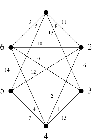
Let $G$ be a finite graph. A labeling of $G$ is an assignment of a nonnegative integer to each edge of $G$. A magic labeling of magic sum $r$ of $G$ is a labeling such that for each vertex $v$ of $G$ the sum of the labels of all edges incident to $v$ is the magic sum $r$ (loops are counted as incident only once) [18, 19, 20, 21]. Graphs with a magic labeling are also called magic graphs (see Figure 1 for an example of a magic labeling of the complete graph $K_{6}$ of magic sum $40$).

We define a magic labeling of a digraph $D$ of magic sum $r$ to be an assignment of a nonnegative integer to each edge of $D$, such that for each vertex $v_{i}$ of $D$, the sum of the labels of all edges with $v_{i}$ as the initial vertex is $r$, and the sum of the labels of all edges with $v_{i}$ as the terminal vertex is also $r$. Thus magic labelings of a digraph is a network flow, where the flow into and out of every vertex, is the magic sum of the labeling. If we consider the labels of the edges of $G$ as variables, the defining magic sum conditions are simply linear equations, and the set of magic labelings of $G$ becomes the set of integral points inside a pointed polyhedral cone $C_{G}$ [15]. Henceforth, we call $C_{G}$ the cone of magic labelings of $G$. A Hilbert basis of $C_{G}$ has the property that any magic labeling of $G$ can be expressed as a linear combination with nonnegative integer coefficients of the elements of the Hilbert basis (see [1], [2], or [15]). An irreducible magic labeling of a graph is a magic labeling that cannot be written as a sum of two other magic labelings. The minimal Hilbert basis of $C_{G}$ is the set of all irreducible magic labelings and is unique [15]. Henceforth, when we refer to the Hilbert basis in this article, we mean the minimal Hilbert basis.

Let $v_{1},v_{2},\dots,v_{n}$ denote the vertices of $G$ and let $e_{i_{1}},e_{i_{2}},\dots,e_{i_{m_{i}}}$ denote the edges of $G$ that are incident to the vertex $v_{i}$ of $G$. Consider the polytope

$${\cal P}_{G}=\{L\in C_{G}\subseteq\mathbb{R}^{q},\hskip 3.61371pt\sum_{j=1}^{m_{i}}L(e_{i_{j}})=1;i=1,\dots,n\}.$$

We will refer to ${\cal P}_{G}$ as the polytope of magic labelings of $G$ and denote $H_{G}(r)$ to be the number of magic labelings of $G$ of magic sum $r$. Then, $H_{G}(r)$ is the Ehrhart quasi-polynomial of ${\cal P}_{G}$ [16].

We define a polytope ${\cal P}_{D}$ of magic labelings of a digraph $D$ as follows. Let $e_{i_{1}},\dots,e_{i_{m_{i}}}$ denote the edges of $D$ that have the vertex $v_{i}$ as the initial vertex and let $f_{i_{1}},f_{i_{2}},\dots,f_{i_{s_{i}}}$ denote the edges of $D$ for which the vertex $v_{i}$ is the terminal vertex, then:

$$\begin{array}[]{l}{\cal P}_{D}=\{L\in C_{D}\subseteq\mathbb{R}^{q},\hskip 3.61371pt\sum_{j=1}^{m_{i}}L(e_{i_{j}})\\ =\sum_{j=1}^{s_{i}}L(f_{i_{j}})=1;i=1,\dots,n\}.\end{array}$$

Let $H_{D}(r)$ denote the number of magic labelings of $D$ of magic sum $r$. Then like before, $H_{D}(r)$ is the Ehrhart quasi-polynomial of ${\cal P}_{D}$. We now connect the magic labelings of digraphs to magic labelings of bipartite graphs.

For example, the magic labelings of the Octahedral digraph with the given orientation $D_{O}$ in Figure 2 are in one-to-one correspondence with the magic labelings of the bipartite graph $G_{D_{O}}$.

A graph $G$ is called a positive graph if for any edge $e$ of $G$ there is a magic labeling $L$ of $G$ for which $L(e)>0$ [18]. Since edges of $G$ that are always labeled zero for any magic labeling of $G$ may be ignored to study magic labelings, we will concentrate on positive graphs in general. We use the following results by Stanley from [18] and [19] to prove Theorems 1.4 and 1.5 and Corollary 1.3.1.

We now conclude that $H_{D}(r)$ is a polynomial for every digraph $D$.

Consider the polytope ${\cal P}:=\{x|Ax\leq b\}$. Let $c$ be a nonzero vector, and let $\delta=$ max $\{cx|Ax\leq b\}$. The affine hyperplane $\{x|cx=\delta\}$ is called a supporting hyperplane of $\cal P$. A subset $F$ of $\cal P$ is called a face of $\cal P$ if $F=\cal P$ or if $F$ is the intersection of $\cal P$ with a supporting hyperplane of $\cal P$. Alternatively, $F$ is a face of $\cal P$ if and only if $F$ is nonempty and

$$F=\{x\in{\cal P}|A^{\prime}x=b^{\prime}\}$$

for some subsystem $A^{\prime}x\leq b^{\prime}$ of $Ax\leq b$. See [15] for basic definitions with regards to polytopes.

Therefore, a face of ${\cal P}_{G}$ is a polytope of the form

$$\{L\in{\cal P}_{G},L(e_{i_{k}})=0;e_{i_{k}}\in E_{0}\},$$

where $E_{0}=\{e_{i_{1}},\dots,e_{i_{r}}\}$ is a subset of the set of edges of $G$.

Observe from Theorem 1.4 that there is an edge between two vertices $v_{i}$ and $v_{j}$ of ${\cal P}_{G}$ if and only if there is a graph with at most $n-b+1$ edges, with magic labelings $v_{i}$ and $v_{j}$. The edge graph of ${\cal P}_{\Gamma_{3}}$ is given in Figure 3. Similarly, we can draw the face poset of ${\cal P}_{G}$ (see Figure 4 for the face poset of ${\cal P}_{\Gamma_{3}}$).

An $n\times n$ semi-magic square of magic sum $r$ is an $n\times n$ matrix with nonnegative integer entries such that the entries of every row and column add to $r$. Doubly stochastic matrices are $n\times n$ matrices in $\mathbb{R}^{n^{2}}$ such that their rows and columns add to 1. The set of all $n\times n$ doubly stochastic matrices form a polytope $B_{n}$, called the Birkhoff polytope. See [7], [8], or [15] for a detailed study of the Birkhoff polytope.

A symmetric magic square is a semi-magic square that is also a symmetric matrix. Let $H_{n}(r)$ denote the number of symmetric magic squares of magic sum $r$ (see [3], [19], and the references therein for the enumeration of symmetric magic squares). We define the polytope ${\cal S}_{n}$ of $n\times n$ symmetric magic squares to be the convex hull of all real nonnegative $n\times n$ symmetric matrices such that the entries of each row (and therefore column) add to one.

A one-to-one correspondence between symmetric magic squares $M=[m_{ij}]$ of magic sum $r$, and magic labelings of the graph $\Gamma_{n}$ of the same magic sum $r$ was established in [19]: let $e_{ij}$ denote an edge between the vertex $v_{i}$ and the vertex $v_{j}$ of $\Gamma_{n}$. Label the edge $e_{ij}$ of $\Gamma_{n}$ with $m_{ij}$, then this labeling is a magic labeling of $\Gamma_{n}$ with magic sum $r$. See Figure 5 for an example. Therefore, we get ${\cal P}_{\Gamma_{n}}$ = ${\cal S}_{n}$ and $H_{\Gamma_{n}}(r)=H_{n}(r)$.

We define a digraph $D$ to be a positive digraph if the corresponding bipartite graph $G_{D}$ is positive.

Let $\Pi_{n}$ denote the complete digraph with $n$ vertices, i.e, there is an edge from each vertex to every other, including the vertex itself (thereby creating a loop at every vertex), then $G_{\Pi_{n}}$ is the the complete bipartite graph $K_{n,n}$. We get a one-to-one correspondence between semi-magic squares $M=[m_{ij}]$ of magic sum $r$ and magic labelings of $\Pi_{n}$ of the same magic sum $r$ by labeling the edges $e_{ij}$ of $\Pi_{n}$ with $m_{ij}$. This also implies that there is a one-to-one correspondence between semi-magic squares and magic labelings of $K_{n,n}$ (this correspondence is also mentioned in [18] and [20]). See Figure 6 for an example.

A good description of the faces of Birkhoff polytope is not known [14]. We can now give an explicit description of the faces of the Birkhoff polytope.

See Figure 7 for the edge graph of $B_{3}$. Two faces of a polytope of magic labelings of a graph (or a digraph) are said to be isomorphic faces if the subgraphs (subdigraphs, respectively) defining the faces are isomorphic. A set of faces is said to be a generating set of $d$-dimensional faces if every $d$-dimensional face is isomorphic to one of the faces in the set. See Figures 8, 9, 10, and 11 for the generators of the edges, the two dimensional faces, the facets, and the Birkhoff polytope $B_{3}$, respectively. The numbers in square brackets in the figures indicate the number of faces in the isomorphism class of the given face.

The proofs of Theorems 1.4 and 1.5, and Corollaries 1.4.1 and 1.5.1 are presented in Section 2.

A polytope $\cal P$ is called rational if each vertex of $\cal P$ has rational coordinates.

An element $\beta$ in the semigroup $S_{C_{G}}$ is said to be completely fundamental, if for any positive integer $n$ and $\alpha,{\alpha}^{\prime}\in S_{C_{G}}$, $n\beta=\alpha+{\alpha}^{\prime}$ implies $\alpha=i\beta$ and ${\alpha}^{\prime}=(n-i)\beta$, for some positive integer $i$, such that $0\leq i\leq n$ (see [17]).

By Lemma 2.2, the dimension of ${\cal P}_{G}$ is $q-n+b$. Therefore, to get a $d$-dimensional polytope, we need to label at least $q-n+b-d$ of $G$ edges always 0. This implies that the $d$-dimensional face is the set of magic labelings of a positive subgraph of $G$ with $n$ vertices and at most $n-b+d$ edges. $\square$

The proof of Theorem 1.4 follows from Lemmas 2.1, 2.2, and 2.3. We can now prove Corollary 1.4.1.

It is clear from the one-to-one correspondence between magic labelings of $\Gamma_{n}$ and symmetric magic squares that ${\cal P}_{\Gamma_{n}}$ has the given description. Since the graph ${\Gamma_{n}}$ has $\frac{n(n+1)}{2}$ edges and $n$ vertices, and every graph is a subgraph of $\Gamma_{n}$, it follows from Theorem 1.4 that the dimension of ${\cal P}_{\Gamma_{n}}$ is $\frac{n(n-1)}{2}$; the $d$-dimensional faces of ${\cal P}_{\Gamma_{n}}$ are $d$-dimensional polytopes of magic labelings of positive graphs with $n$ vertices and at most $n+d$ edges.

We can partition the vertices of $\Gamma_{2n}$ into two equal sets $A$ and $B$ in ${2n-1}\choose n$ ways: Fix the vertex $v_{1}$ to be in the set $A$ , then we can choose the n vertices for the set $B$ in ${2n-1}\choose n$ ways, and the remaining $n-1$ vertices will belong to the set $A$. By adding the required edges, we get a complete bipartite graph for every such partition of the vertices of $\Gamma_{2n}$. Thus, the number of subgraphs of $\Gamma_{2n}$ that are isomorphic to $K_{n,n}$ is ${2n-1}\choose n$. Therefore, there are $2n-1\choose n$ faces of ${\cal P}_{\Gamma_{2n}}$ that are Birkhoff polytopes because every isomorphic copy of $K_{n,n}$ contributes to a face of ${\cal P}_{\Gamma_{2n}}$. $\square$

Since the edges with nonzero labels are the same for both $L$ and $L^{\prime}$, it follows that the magic sums are also the same. $\square$

Similarly, we can prove:

We now prove our results about polytope of magic digraphs.

We derive our results about the faces of the Birkhoff polytope as a consequence.

Proof of Corollary 1.5.1. The one-to-one correspondence between semi-magic squares and magic labelings of ${\Pi_{n}}$ gives us that ${\cal P}_{\Pi_{n}}=B_{n}$. Since every digraph with $n$ vertices is a subgraph of $\Pi_{n}$, by Theorem 1.5, it follows that its $d$-dimensional faces are $d$-dimensional polytopes of magic labelings of positive digraphs with $n$ vertices and at most $2n-1+d$ edges. Since the vertex set of a face of $B_{n}$ is a subset of the vertex set of $B_{n}$ it follows that the vertices of ${\cal P}_{D}$, where $D$ is a positive digraph, are permutation matrices. $\square$

In this section, we present some examples and applications of magic graphs. Interesting examples of magic digraphs are Cayley digraphs of finite groups. Let $G$ be a finite group $\{g_{1},g_{2},\dots,g_{n}=I\}$. The Cayley group digraph of $G$ is a graphical representation of $G$: every element $g_{i}$ of the group $G$ corresponds to a vertex $v_{i}$ $(i=1,2,\dots,n)$ and every pair of distinct vertices $v_{i},v_{j}$ is joined by an edge labeled with $\alpha$ where $g_{\alpha}=g_{j}g_{i}^{-1}$ [12]. For example, the Cayley digraph for the permutation group

$$\begin{array}[]{l}S_{3}=\{g_{1}=(123),g_{2}=(132),g_{3}=(23),\\ g_{4}=(12),g_{5}=(13),g_{6}=I\}\end{array}$$

is given in Figure 12.

A digraph is called Eulerian if for each vertex $v$ the indegree and the outdegree of $v$ is the same. Therefore, Eulerian digraphs can also be studied as magic digraphs where all the edges are labeled by 1 (see [4] for the applications of Eulerian digraphs to digraph colorings). An $n$-matching of $G$ is a magic labeling of $G$ with magic sum at most $n$ and the labels are from the set $\{0,1,\dots,n\}$ (see [13], chapter 6). A perfect matching of $G$ is a 1-matching of $G$ with magic sum 1.

Hilbert basis can also be used to study factorizations of labeled graphs. We define Factors of a graph $G$ with a labeling $L$ to be labelings $L_{i},i=1,\dots,r$ of $G$ such that $L(G)=\sum_{i=1}^{r}L_{i}(G)$, and if $L_{i}(e_{k})\neq 0$ for some edge $e_{k}$ of $G$, then $L_{j}(e_{k})=0$ for all $j\neq i$. A decomposition of $L$ into factors is called a factorization of $G$. An example of a graph factorization is given in Figure 13. See Chapters 11 and 12 of [12] for a detailed study of graph factorizations.

Our results enable us to reprove some known facts about the Birkhoff polytope as well. For example, Theorem 1.5 gives us that the dimension of $B_{n}$ is ${(n-1)}^{2}$. The leading coefficient of the Ehrhart polynomial of $B_{n}$ is the volume of $B_{n}$. This number has been computed for $n=1,2,\dots,9$ (see [5] and [9]).

The software 4ti2 [11] can be used to find the Hilbert bases of $C_{G}$, and the software LattE [10] can be used to compute the generating functions of $H_{G}(r)$ effectively. See [3] for other results about magic labelings of graphs. See [22] for a study of other types of magic graphs.

References

- [1] Ahmed, M., De Loera, J., and Hemmecke, R., Polyhedral cones of magic cubes and squares, New Directions in Computational Geometry, The Goodman-Pollack Festschrift volume, Aronov et al., eds., Springer-Verlag, 2003, 25–41.
- [2] Ahmed, M., How many squares are there, Mr. Franklin?: Constructing and Enumerating Franklin Squares, Amer. Math. Monthly, Vol.111, 2004, 394-410.
- [3] , Algebraic combinatorics of magic squares, Dissertation, UC Davis, 2004.
- [4] Alon, N., Tarsi, M., A note on graph colorings and graph polynomials, J. Combin. Theory Ser. B 70 (1997), no. 1, 197–201.
- [5] Beck, M. and Pixton, D., The Ehrhart polynomial of the Birkhoff polytope, to appear in Discrete and computational geometry, Springer-Verlag, New York.
- [6] Beck, M., Cohen, M., Cuomo, J., and Gribelyuk, P., The number of magic squares, cubes and hypercubes, Amer. Math. Monthly, Vol.110, no.8, (2003), 707-717.
- [7] Billera, L.J. and Sarangarajan, A., The combinatorics of permutation polytopes, Formal power series and algebraic combinatorics, New Brunswick, NJ, 1994, 1–23, DIMACS Ser. Discrete Math. Theoret. Comput. Sci., Vol.24, Amer. Math. Soc., Providence, RI, 1996.
- [8] Brualdi, A. R., and Gibson, P., Convex polyhedra of doubly stochastic matrices: I, II, III, Journal of combinatorial Theory, A22, 1977, 467-477.
- [9] Chan, S. C. and Robbins, D. P., On the volume of the polytope of doubly stochastic matrices, Experiment. Math., Vol. 8, no.3, 1999, 291-300.
- [10] De Loera, J., Hemmecke, R., Tauzer, J., and Yoshida, R., Effective lattice point counting in rational convex polytopes, to appear in the Journal of Symbolic Computation; software implementation LattE is available from http://www.math.ucdavis.edu/ latte.
- [11] Hemmecke, R., On the computation of Hilbert bases of cones, in Proceedings of First International Congress of Mathematical Software, A. M. Cohen, X.S. Gao, and N. Takayama, eds., Beijing, (2002); software implementation 4ti2 is available from http://www.4ti2.de.
- [12] König, D., Theory of finite and infinite graphs, Birkhäuser Boston, 1990.
- [13] Lov́asz, L. and Plummer, M. D., Matching Theory, North-Holland, Amsterdam, 1986.
- [14] Pak, I., On the number of faces of certain transportation polytopes, European J. Combinatorics, vol. 21, 2000, 689-694.
- [15] Schrijver, A., Theory of Linear and Integer Programming, Wiley-Interscience, 1986.
- [16] Stanley, R.P., Enumerative Combinatorics, Volume I, Cambridge, 1997.
- [17] , Combinatorics and commutative algebra, Progress in Mathematics, 41, Birkhaüser Boston, MA, 1983.
- [18] ) , Linear Homogeneous Diophantine Equations and Magic Labelings Of Graphs, Duke Mathematical Journal, Vol.40, September 1973, 607-632.
- [19] , Magic Labelings of Graphs, Symmetric Magic Squares, Systems of Parameters and Cohen-Macaulay Rings, Duke Mathematical Journal, Vol.43, No.3, September 1976, 511-531.
- [20] Stewart, B. M., Magic graphs, Canad. J. Math., vol. 18, 1966, 1031-1059.
- [21] , Supermagic complete graphs, Canad. J. Math., vol. 19, 1967, 427-438.
- [22] Wallis, D., Magic Graphs, Birkhäuser Boston, 2001.