¹¹footnotetext: Partially supported by the DAAD fellowship (Germany), the Golda Meir postdoctoral fellowship (the Einstein mathematics institute, Hebrew university, Jerusalem), the Emmy Noether Research Institute for Mathematics (center of the Minerva Foundation of Germany), the Excellency Center ”Group Theoretic Methods in the Study of Algebraic Varieties” of the Israel Science Foundation, and EAGER (EU network, HPRN-CT-2009-00099).

Braid monodromy factorization for a non-prime $K3$ surface branch curve

Amram Meirav¹, Ciliberto Ciro, Miranda Rick and Teicher Mina Address: Meirav Amram, Mathematisches Institut, Bismarck Strasse 1 1/2, Erlangen, Germany; Einstein Institute for Mathematics, Hebrew University, Jerusalem Email address: meirav@macs.biu.ac.il/ameirav@math.huji.ac.il Address: Ciro Ciliberto, Dipartimento di Matematica, Universita di Roma II, Tor Vergata, 00123 Roma, Italy Email address: cilibert@mat.uniroma2.it Address: Rick Miranda, Department of Mathematics, Colorado State University, Fort Collins, CO 80523 USA Email address: rick.miranda@colostate.edu Address: Mina Teicher, Department of Mathematics, Bar-Ilan university, 52900 Ramat-Gan, Israel Email address: teicher@macs.biu.ac.il

Date: August 11, 2026

Abstract.

In this paper we consider a non-prime $K3$ surface of degree $16$ , and study a specific degeneration of it, known as the $(2,2)$ -pillow degeneration, [10].

We study also the braid monodromy factorization of the branch curve of the surface with respect to a generic projection onto ${\mathbb{C}}{\mathbb{P}}^{2}$ .

In [4] we compute the fundamental groups of the complement of the branch curve and of the corresponding Galois cover of the surface.

Key words and phrases:

K3

surfaces, degeneration, generic projection, branch curve, braid monodromy, classification of surfaces. AMS classification numbers. 14D05, 14D06, 14E25, 14J10, 14J28, 14Q05, 14Q10.

1. Overview

Given a projective surface and a generic projection to the plane, the fundamental group of the complement of the branch curve is one of its most important invariants. Our goal is to compute this group and the fundamental group of the Galois cover (which is known to be a certain quotient of the fundamental group of the complement of the branch curve, see [13]). This goal is achieved in [4].

In this paper we deal with a non-prime $K3$ surface of degree 16 which is embedded in ${\mathbb{P}}^{9}$ . In order to compute the above groups we degenerate the surface into a union of 16 planes. We then project it onto ${\mathbb{C}}{\mathbb{P}}^{2}$ to get a degenerated branch curve $S_{0}$ , from which one can compute the braid monodromy factorization and the branch curve $S$ of the projection of the original $K3$ surface. With this information we will be able to apply the van Kampen Theorem (see [20]) and the regeneration rules (see [18]) to get presentations for the relevant fundamental groups.

The idea of using degenerations for these purposes appears already in [3], [9], [11], [13] and [17]. Degenerations of $K3$ surfaces, of which the one we use here is an example, were constructed in [10] and are called pillow degenerations.

The study of braids was begun by Artin in [1] and [2]; see also Chisini [8]. The braid monodromy technique was first presented by Moishezon-Teicher in [12], [14] and [15]. Many examples of computations of braid monodromy have been executed, see for example in [3], [5], [15]. Also in [7] one can find a description of computations of braid monodromy and the fundamental group $\pi_{1}({\mathbb{C}}{\mathbb{P}}^{2}-S)$ of the complement of the branch curve of a surface. In this work we encounter new type of singularities ( $3$ -points, see Section 4.2.1) which have not been handled before, whose analysis is necessary to give the precise computations of the braid monodromy. Moreover, since the monodromies related to $6$ -points are quite hard to follow, we present them first in a precise way algebraically, followed then by figures which illustrate the computations.

In [7], the authors also considered the branch curve of a projection of a non-prime $K3$ surface. But they considered quotients of $\pi_{1}({\mathbb{C}}{\mathbb{P}}^{2}-S)$ (where $S$ is the branch curve) by a subgroup of commutators (commutators of geometric generators which are mapped to disjoint transpositions by the geometric monodromy representation, see Definition 2.2 in that paper). Their motivation came from the theory of symplectic manifolds and families of projections where the branch curves acquire and may lose pairs of transverse double points with opposite orientations; creating a pair of double points adds a commutation relation. The quotient there is the largest quotient of $\pi_{1}({\mathbb{C}}{\mathbb{P}}^{2}-S)$ , which is guaranteed to be invariant under these operations, and it is different from the $\pi_{1}({\mathbb{C}}{\mathbb{P}}^{2}-S)$ or the group related to the fundamental group of the Galois cover, which is our aim (see [4]).

The paper is divided as follows. In Section 2 we give the definition of a degeneration and explain briefly the computations from [10]. In Section 3 we review the general setup and the notion of the braid monodromy. In Section 4 we recover the relevant properties of the branch curve $S$ of the generic projection to the plane of the $K3$ surface by using regeneration techniques. Section 5 states the braid monodromy factorization of $\Delta_{48}^{2}$ of $S$ and its related invariance properties. We explain why the computations of $\Delta_{48}^{2}$ and its invariance are necessary for this work and for future work.

2. $K3$ surfaces and their degenerations

2.1. $K3$ surfaces

Compact complex surfaces are classified into four broad categories, based on the growth rate of sections of powers of the canonical class. Such sections can either be always zero (rational or ruled surfaces); form vector spaces of bounded dimension, or have spaces of sections whose dimensions grow linearly (elliptic surfaces) or quadratically (surfaces of general type) with the power. For surfaces for which these sections are bounded, some multiple of the canonical bundle is trivial, and there are nine separate families up to complex deformation. The surfaces of this type which are simply connected in fact have trivial canonical bundle, and are called $K3$ surfaces; the invariants for such surfaces are $p_{g}=1$ , $q=0$ , $e=24$ , and $h^{1,1}=22$ , see [9] and [10]. The most common example of a $K3$ surface is a smooth quartic surface in $\mathbb{P}^{3}$ . The moduli space of all $K3$ surfaces is $20$ -dimensional.

Most $K3$ surfaces are not algebraic; the algebraic ones are classified by an infinite collection (depending on an integer $g\geq 2$ ) of $19$ -dimensional moduli spaces. The general member of the family has a rank one Picard group, generated by an ample class $H$ with $H^{2}=2g-2$ ; the general member of the linear system $|H|$ is a smooth curve of genus $g$ , and this linear system maps the $K3$ surface to $\mathbb{P}^{g}$ as a surface of degree $2g-2$ . For example, the quartic surfaces in $\mathbb{P}^{3}$ form the family with $g=3$ . The integer $g$ is called the genus of the family.

The $K3$ surfaces may also be embedded by a multiple $cH$ of the primitive class $H$ ; this will exhibit the family of $K3$ surfaces of genus $g$ as surfaces of degree $D=c^{2}(2g-2)$ in $\mathbb{P}^{G}$ , where $G=1+c^{2}(g-1)$ , whose hyperplane section is an element of $|cH|$ , and therefore is a curve of genus $G$ .

2.2. Degenerations of $K3$ surfaces

Let us start this section with recalling the definition of degeneration from [17].

Definition 1.

Projective degeneration Let $\Delta$ be the unit disc, and $X,Y$ be algebraic surfaces (or more generally algebraic varieties). Suppose that $k:Y\rightarrow{\mathbb{C}}{\mathbb{P}}^{n}$ and $k^{\prime}:X\rightarrow{\mathbb{C}}{\mathbb{P}}^{n}$ are projective embeddings. We say that $k^{\prime}$ is a projective degeneration of $k$ if there exist a flat family $\pi:V\rightarrow\Delta$ , and an embedding $F:V\rightarrow\Delta\times{\mathbb{C}}{\mathbb{P}}^{n}$ , such that $F$ composed with the first projection is $\pi$ , and:

(a)

$\pi^{-1}(0)\simeq X$ ;
(b)

there is a $t_{0}\neq 0$ in $\Delta$ such that $\pi^{-1}(t_{0})\simeq Y$ ;
(c)

the family $V-\pi^{-1}(0)\rightarrow\Delta-{0}$ is smooth;
(d)

restricted to $\pi^{-1}(0)$ , $F={0}\times k^{\prime}$ under the identification of $\pi^{-1}(0)$ with $X$ ;
(e)

restricted to $\pi^{-1}(t_{0})$ , $F={t_{0}}\times k$ under the identification of $\pi^{-1}(t_{0})$ with $Y$ .

In [10], the authors constructed a degeneration of embedded $K3$ surfaces, to a union of $D$ planes, meeting according to the combinatorics of a certain triangulation of the $2$ -sphere. Such degenerations are called Type III degenerations, and there are many such available. The particular one constructed there was formed by first decomposing the sphere into two rectangles, then decomposing each rectangle into $ab$ squares (by decomposing the sides of the rectangles into $a$ and $b$ line segments), and finally decomposing each square into two triangles (planes). The parameters $a$ and $b$ are free to choose, and the construction exhibits a degeneration of $K3$ surfaces into $4ab$ planes. If $c$ is the greatest common divisor of $a$ and $b$ , the general member of the family is a smooth $K3$ surface embedded by the multiple $c$ of the generator $H$ of the Picard group. Hence using the above notation, $4ab=2c^{2}(g-1)$ , so that $g=1+2(ab/c^{2})$ and $G=1+2ab$ (the number of coordinate points in ${\mathbb{P}}^{G}$ is $G+1$ ). The boundary of the two rectangular arrays of planes contains $2a+2b$ lines, where the identification is taking place.

This degeneration of a $K3$ surface, is called a pillow degeneration, see [10].

This article proceeds by making further analyses with the $a=b=2$ case. Given a non-prime $K3$ surface of degree $16$ , we get the pillow degeneration $(K3)_{0}$ , as depicted in Figure 1. We quote the main result from [10].

Theorem 2.

The $(2,2)$ -pillow degeneration $(K3)_{0}$ is a total degeneration of a smooth $K3$ surface of degree $16$ in ${\mathbb{P}}^{9}$ . The smooth $K3$ surface is a re-embedding of a quartic surface in ${\mathbb{P}}^{3}$ via the linear system of quadrics.

Refer to caption — Figure 1. The $(2,2)$ -pillow degeneration

For the regeneration process we have to fix a numbering of the vertices and lines. The boundary points are labeled from $1$ to $8$ , while the interior point on the top is $9$ and on the bottom is $10$ . The $16$ planes meet each other along a total of $24$ lines, each joining two of the $10$ coordinate points. The numbering of the vertices induces a lexicographic numbering of the lines as follows. If $L$ has endpoints $a<b$ and $M$ has endpoints $c<d$ then $L<M$ if $b<d$ or $d=b$ and $a<c$ . This gives a total ordering of the lines, which we interpret as a numbering from $1$ to $24$ , as shown in Figure 1.

Note that the coordinate points $1$ , $3$ , $6$ , and $8$ at the corners are each contained in three distinct planes, while all other points are each contained in six planes. We call these two types $3$ -points and $6$ -points respectively.

A general projection $f_{0}:(K3)_{0}\to{\mathbb{C}}{\mathbb{P}}^{2}$ will also be a degeneration of a general such projection of the smooth $K3$ surface. Under $f_{0}$ , each of the $16$ planes is mapped isomorphically to ${\mathbb{C}}{\mathbb{P}}^{2}$ . The ramification locus $R_{0}$ of $f_{0}$ is the closed subset of $(K3)_{0}$ , where $f_{0}$ is not a local isomorphism. Here $R_{0}$ is exactly the $24$ lines. Let $S_{0}=f_{0}(R_{0})$ be the degenerated branch curve; it is a line arrangement, composed of the images of the $24$ lines (each counted twice and each of which is a line in the plane).

3. The braid monodromy notion

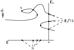
Consider the following setting (Figure 2). $S$ is an algebraic curve in ${\mathbb{C}}^{2}$ , with $p=\deg(S)$ . Let $\pi:{\mathbb{C}}^{2}\rightarrow{\mathbb{C}}$ be a generic projection onto the first coordinate. Define the fiber $K(x)=\{y\mid(x,y)\in S\}$ in $S$ over a fixed point $x$ , projected to the $y$ -axis. Define $N=\{x\mid\#K(x)<p\}$ and $M^{\prime}=\{s\in S\mid\pi_{\mid s}\mbox{ is not \'{e}tale at }s\}$ ; note that $\pi(M^{\prime})=N$ . Let ${\{{A_{j}}\}}^{q}_{j=1}$ be the set of points of $M^{\prime}$ and $N={\{{x_{j}}\}}^{q}_{j=1}$ their projection on the $x$ -axis. Recall that $\pi$ is generic, so we assume that $\#(\pi^{-1}(x)\cap M^{\prime})=1$ for every $x\in N$ . Let $E$ (resp. $D$ ) be a closed disk on the $x$ -axis (resp. the $y$ -axis), such that $M^{\prime}\subset E\times D$ and $N\subset\mbox{Int}(E)$ . We choose $u\in\partial E$ a real point far enough from the set $N$ , so that $x<<u$ for every $x\in N$ . Define ${\mathbb{C}}_{u}=\pi^{-1}(u)$ and number the points of $K={\mathbb{C}}_{u}\cap S$ as $\{1,\dots,p\}$ .

We now construct a g-base for the fundamental group $\pi_{1}(E-N,u)$ . Take a set of paths ${\{{\gamma_{j}}\}}^{q}_{j=1}$ which connect $u$ with the points ${\{{x_{j}}\}}^{q}_{j=1}$ of $N$ . Now encircle each $x_{j}$ with a small oriented counterclockwise circle $c_{j}$ . Denote the path segment from $u$ to the boundary of this circle as $\gamma^{\prime}_{j}$ . We define an element (a loop) in the g-base as $\delta_{j}={\gamma^{\prime}}_{j}c_{j}{\gamma^{\prime}}^{-1}_{j}$ . Let $B_{p}[D,K]$ be the braid group, and let $H_{1},\dots,H_{p-1}$ be its frame (for complete definitions, see [14, Section III.2]). The braid monodromy of $S$ [2] is a map $\varphi:\pi_{1}(E-N,u)\rightarrow B_{p}[D,K]$ defined as follows: every loop in $E-N$ starting at $u$ has liftings to a system of $p$ paths in $(E-N)\times D$ starting at each point of $K=1,\ldots,p$ . Projecting them to $D$ we obtain $p$ paths in $D$ defining a motion $\{1(t),\dots,p(t)\}$ (for $0\leq t\leq 1$ ) of $p$ points in $D$ starting and ending at $K$ . This motion defines a braid in $B_{p}[D,K]$ . By the Artin Theorem [15], for $j=1,\dots,q$ , there exists a halftwist $Z_{j}\in B_{p}[D,K]$ and $\epsilon_{j}\in{\mathbb{Z}}$ , such that $\varphi(\delta_{j})=Z_{j}^{\epsilon_{j}}$ , where $Z_{j}$ is a halftwist and $\epsilon_{j}=1,2$ or $3$ (for an ordinary branch point, a node, or a cusp respectively). We now explain how to describe this $Z_{j}$ .

First we recall a definition of an almost real curve from [15], as we have such curves here.

Definition 3.

A curve $S$ is called an almost real curve if

(1)

$N\subseteq E\cap{\mathbb{R}}$ ,
(2)

$N\subset E-\partial E$ ,
(3)

$\forall x\in{E\cap{\mathbb{R}}-N},\#{(K\cap{\mathbb{R}})(x)}\geq p-1$ ,
(4)

$\forall x\in N,\#{\pi^{-1}(x)\cap M^{\prime}}=1$ ,
(5)
The singularities can be
1. (a)
  
  a branch point, topologically locally equivalent to $y^{2}+x=0$ or $y^{2}-x=0$ ,
2. (b)
  
  a tacnode (a line is tangent to a conic)
3. (c)
  
  an intersection of $m$ smooth branches, transversal to each other.

We explain how to get the braid monodromy around each singularity in $S$ . Let $A_{j}$ be a singularity in $S$ and denote by $x_{j}$ its projection by $\pi$ to the $x$ -axis. We choose a point $x^{\prime}_{j}$ next to $x_{j}$ , such that $\pi^{-1}(x^{\prime}_{j})$ is a typical fiber. If $A_{j}$ is (b), (c) or (d), then $x^{\prime}_{j}$ is on the right side of $x_{j}$ . If $A_{j}$ is (a), then $x^{\prime}_{j}$ is on the left side of $x_{j}$ (the typical fiber in case (a), which is on the left side of this singularity, intersects the conic in two real points). We encircle $A_{j}$ with a very small circle in such a way that the typical fiber $\pi^{-1}(x^{\prime}_{j})$ intersects the circle in two points, say $a,b$ . We fix a skeleton $\xi_{x^{\prime}_{j}}$ which connects $a$ and $b$ , and denote it as $<a,b>$ . The Lefschetz diffeomorphism $\Psi$ ([3, Subsection 1.9.5]) allows us to get a resulting skeleton $(\xi_{x^{\prime}_{j}})\Psi$ in the typical fiber ${\mathbb{C}}_{u}$ . This one defines a motion of its two endpoints. This motion induces a halftwist $Z_{j}=\Delta<(\xi_{x^{\prime}_{j}})\Psi>$ . As above, $\varphi(\delta_{j})=\Delta<(\xi_{x^{\prime}_{j}})\Psi>^{\epsilon_{j}}$ . The braid monodromy factorization associated to $S$ is

\Delta^{2}_{p}=\prod\limits^{q}_{j=1}\varphi(\delta_{j}).

4. The branch curve $S_{0}$ and its regeneration

4.1. The branch curve $S_{0}$

The degenerated object $(K3)_{0}$ has $\{j\}^{10}_{j=1}$ as vertices. By the projection $f_{0}:K3_{0}\rightarrow{\mathbb{C}}{\mathbb{P}}^{2}$ , we obtain a line arrangement $S_{0}=\bigcup\limits^{24}_{i=1}L_{i}$ , and the projections $f_{0}(j)=j$ are singularities of $S_{0}$ . The $3$ -points are $1,3,6,8$ and the $6$ -points are $2,4,5,7,9,10$ . In the following subsection we regenerate in neighborhoods of these singularities. The monodromies will be given in the next section.

Besides these singularities in $S_{0}$ , there are also parasitic intersections: these come from lines in $(K3)_{0}$ which do not intersect, but when projecting $(K3)_{0}$ onto ${\mathbb{C}}{\mathbb{P}}^{2}$ , they will intersect. Denote each line in $(K3)_{0}$ as a pair (by its two end vertices). Let $u$ be a point, $u\notin S_{0}$ , such that $\#{\mathbb{C}}_{u}=24$ , and $q_{i}=i\cap{\mathbb{C}}_{u}$ a real point. Take two non-intersecting lines $p=(i,k)$ and $t=(j,\ell)$ in $(K3)_{0}$ .

Notation 4.

We denote by $Z_{ij}$ (resp. $\bar{Z}_{ij}$ ) the counterclockwise halftwist of $i$ and $j$ along a path below (resp. above) the real axis. If $P$ is a set of points between $i$ and $j$ , $\stackrel{{\scriptstyle(P)}}{{Z_{ij}}}$ denotes the path from $i$ to $j$ going above the points in $P$ and below the points not in $P$ . Conjugation of braids is defined as $a^{b}=b^{-1}ab$ .

We first compute the products $D_{t}:=\prod\limits_{\stackrel{{\scriptstyle p<t}}{{p\cap t=\emptyset}}}\tilde{Z}^{2}_{pt}$ as explained in [14, Theorem IX.2.1].

	$\displaystyle\ D_{1}=$	$\displaystyle D_{2}=D_{4}=Id\ ,\ D_{3}={Z}^{2}_{2\;3}\ ,\ \ D_{5}=\bar{Z}^{2}_{3\;5}\ ,\ \ D_{6}=\prod\limits_{i=1,3,4}\mathop{\lower 10.0pt\hbox{${\mathrel{\mathop{\kern 0.0pt\hskip-5.69046pt\scriptstyle{(5)}}\limits^{\displaystyle\bar{Z}^{2}_{i\;6}}}}$}}\nolimits\ ,\ \ D_{7}=\prod\limits_{i=1,2,5,6}\;\;\ \bar{Z}^{2}_{i\;7}$
	$\displaystyle\ D_{8}=$	$\displaystyle\prod\limits_{i=1,2,5,6}\bar{Z}^{2}_{i\;8}\ ,\ \ D_{9}=\prod\limits_{i=1-4,7}\;\mathop{\lower 10.0pt\hbox{${\mathrel{\mathop{\kern 0.0pt\hskip-5.69046pt\scriptstyle{(8)}}\limits^{{\displaystyle\bar{Z}^{2}_{i\;9}}}}}$}}\nolimits\ ,\ \ D_{10}=\prod\limits_{i=1}^{6}\;\mathop{\lower 10.0pt\hbox{${\mathrel{\mathop{\kern 0.0pt\hskip-5.69046pt\scriptstyle{(8)(9)}}\limits^{{\displaystyle\bar{Z}^{2}_{i\;10}}}}}$}}\nolimits\ ,\ \ D_{11}=\prod\limits_{i=1-4,7,8,10}\;\;\bar{Z}^{2}_{i\;11}\ ,$
	$\displaystyle\ D_{12}=$	$\displaystyle\prod\limits^{7}_{i=1}\;\;\mathop{\lower 10.0pt\hbox{${\mathrel{\mathop{\kern 0.0pt\hskip-5.69046pt\scriptstyle{(11)}}\limits^{{\displaystyle\bar{Z}^{2}_{i\;12}}}}}$}}\nolimits\ ,\ \ D_{13}=\prod\limits^{12}_{\stackrel{{\scriptstyle\scriptstyle i=3}}{{\scriptstyle i\neq 4,5}}}\;\bar{Z}^{2}_{i\;13}\ ,\ \ D_{14}=\prod\limits^{12}_{\stackrel{{\scriptstyle\scriptstyle i=1}}{{\scriptstyle i\neq 2,6}}}\;\;\mathop{\lower 10.0pt\hbox{${\mathrel{\mathop{\kern 0.0pt\hskip-5.69046pt\scriptstyle{(13)}}\limits^{{\displaystyle\bar{Z}^{2}_{i\;14}}}}}$}}\nolimits\ ,\ \ D_{15}=\prod\limits^{12}_{\stackrel{{\scriptstyle\scriptstyle i=1}}{{\scriptstyle i\neq 3,4,7,8}}}\;\;\mathop{\lower 10.0pt\hbox{${\mathrel{\mathop{\kern 0.0pt\hskip-5.69046pt\scriptstyle{(13)(14)}}\limits^{{\displaystyle\bar{Z}^{2}_{i\;15}}}}}$}}\nolimits\ ,$
	$\displaystyle\ D_{16}=$	$\displaystyle\prod\limits^{12}_{\stackrel{{\scriptstyle\scriptstyle i=1}}{{\scriptstyle i\neq 5,6,9,11}}}\;\;\mathop{\lower 10.0pt\hbox{${\mathrel{\mathop{\kern 0.0pt\hskip-5.69046pt\scriptstyle{(13)-(15)}}\limits^{{\displaystyle\bar{Z}^{2}_{i\;16}}}}}$}}\nolimits\ ,\ \ D_{17}=\prod\limits^{12}_{\stackrel{{\scriptstyle\scriptstyle i=1}}{{\scriptstyle i\neq 7,10}}}\;\;\mathop{\lower 10.0pt\hbox{${\mathrel{\mathop{\kern 0.0pt\hskip-5.69046pt\scriptstyle{(13)-(16)}}\limits^{{\displaystyle\bar{Z}^{2}_{i\;17}}}}}$}}\nolimits\ ,\ \ D_{18}=\prod\limits^{11}_{\stackrel{{\scriptstyle\scriptstyle i=1}}{{\scriptstyle i\neq 8-10}}}\;\;\mathop{\lower 10.0pt\hbox{${\mathrel{\mathop{\kern 0.0pt\hskip-5.69046pt\scriptstyle{(13)-(17)}}\limits^{{\displaystyle\bar{Z}^{2}_{i\;18}}}}}$}}\nolimits\ ,\ \ D_{19}=\prod\limits^{18}_{\stackrel{{\scriptstyle\scriptstyle i=2}}{{\scriptstyle i\neq 3}}}\;\bar{Z}^{2}_{i\;19}\ ,$
	$\displaystyle\ D_{20}=$	$\displaystyle\prod\limits^{18}_{\stackrel{{\scriptstyle\scriptstyle i=3}}{{\scriptstyle i\neq 4,5,13}}}\;\;\mathop{\lower 10.0pt\hbox{${\mathrel{\mathop{\kern 0.0pt\hskip-5.69046pt\scriptstyle{(19)}}\limits^{{\displaystyle\bar{Z}^{2}_{i\;20}}}}}$}}\nolimits\ ,\ \ D_{21}=\prod\limits^{18}_{\stackrel{{\scriptstyle\scriptstyle i=1}}{{\scriptstyle i\neq 3,4,7,8,15}}}\;\;\mathop{\lower 10.0pt\hbox{${\mathrel{\mathop{\kern 0.0pt\hskip-5.69046pt\scriptstyle{(19)(20)}}\limits^{{\displaystyle\bar{Z}^{2}_{i\;21}}}}}$}}\nolimits\ ,\ \ D_{22}=\prod\limits^{18}_{\stackrel{{\scriptstyle\scriptstyle i=1}}{{\scriptstyle i\neq 5,6,9,11,16}}}\;\;\mathop{\lower 10.0pt\hbox{${\mathrel{\mathop{\kern 0.0pt\hskip-5.69046pt\scriptstyle{(19)-(21)}}\limits^{{\displaystyle\bar{Z}^{2}_{i\;22}}}}}$}}\nolimits\ ,$
	$\displaystyle\ D_{23}=$	$\displaystyle\prod\limits^{17}_{\stackrel{{\scriptstyle\scriptstyle i=1}}{{\scriptstyle i\neq 8-10,12}}}\;\;\mathop{\lower 10.0pt\hbox{${\mathrel{\mathop{\kern 0.0pt\hskip-5.69046pt\scriptstyle{(19)-(22)}}\limits^{{\displaystyle\bar{Z}^{2}_{i\;23}}}}}$}}\nolimits\ ,\ \ D_{24}=\prod\limits^{18}_{\stackrel{{\scriptstyle\scriptstyle i=1}}{{\scriptstyle i\neq 11,12}}}\;\;\mathop{\lower 10.0pt\hbox{${\mathrel{\mathop{\kern 0.0pt\hskip-5.69046pt\scriptstyle{(19)-(23)}}\limits^{{\displaystyle\bar{Z}^{2}_{i\;24}}}}}$}}\nolimits.$

Define the parasitic intersection braids as

(1)

\tilde{C}_{j}=\prod\limits_{j\in t}D_{t},

where $j$ is the smallest endpoint in the line $t$ . In our case, $\tilde{C}_{1}=D_{1}\cdot D_{3}\cdot D_{19},\ \ \tilde{C}_{2}=D_{2}\cdot D_{4}\cdot D_{5}\cdot D_{13}\cdot D_{20},\ \ \tilde{C}_{3}=D_{6}\cdot D_{14},\ \ \tilde{C}_{4}=D_{7}\cdot D_{8}\cdot D_{15}\cdot D_{21},\ \ \tilde{C}_{5}=D_{9}\cdot D_{11}\cdot D_{16}\cdot D_{22},\ \ \tilde{C}_{6}=D_{10}\cdot D_{17},\ \ \tilde{C}_{7}=D_{12}\cdot D_{18}\cdot D_{23},\ \ \tilde{C}_{8}=D_{24},\ \ \tilde{C}_{9}=\tilde{C}_{10}=Id.$

4.2. The regeneration of $S_{0}$

The degenerated branch curve $S_{0}$ of $(K3)_{0}$ has degree $24$ . However each of the $24$ lines of $S_{0}$ should be counted as a double line in the scheme-theoretic branch locus, since it arises from a line of nodes. Another way to see this is to note that the regeneration of $(K3)_{0}$ induces a regeneration of $S_{0}$ in such a way that each point, say $c$ , on the typical fiber is replaced by two nearby points $c,c^{\prime}$ .

The curve $S_{0}$ has $3$ -points, $6$ -points and parasitic intersections. In the forthcoming subsections we explain how to regenerate the curve in neighbourhoods of these points. The resulting branch curve $S$ will have degree $48$ .

4.2.1. Regeneration of $3$ -points

The $3$ -points in $S_{0}$ are $1,3,6,8$ , see Figure 1. The regeneration is divided into steps. We explain each step in two levels, first dealing with the surface and then with the branch curve.

In the surface level, each diagonal is replaced with a conic by a partial regeneration. Focusing on a $3$ -point, we have a partial regeneration of two of the planes to a quadric surface. We get one quadric and one plane, which is tangent to the quadric. The plane and the quadric meet along two lines (one from each ruling of the quadric).

For the regeneration of the branch curve, we need the following lemma from [18].

Lemma 5.

Let $V$ be a projective algebraic surface, and $D^{\prime}$ be a curve in $V$ . Let $f:V\rightarrow{\mathbb{C}}{\mathbb{P}}^{2}$ be a generic projection. Let $S\subseteq{\mathbb{C}}{\mathbb{P}}^{2},S^{\prime}\subset V$ be the branch curve of $f$ and the corresponding ramification curve. Assume $S^{\prime}$ intersects $D^{\prime}$ at a point $\alpha^{\prime}$ . Let $D=f(D^{\prime})$ and $\alpha=f(\alpha^{\prime})$ . Assume that there exist neighbourhoods of $\alpha$ and $\alpha^{\prime}$ , such that $f_{\mid_{S^{\prime}}}$ and $f_{\mid_{D^{\prime}}}$ are isomorphisms. Then $D$ is tangent to $S$ at $\alpha$ .

At the branch curve level, we have two double lines (coming from the intersection of the plane and the quadric) and one conic (coming from the branching of the quadric over the plane). According to the above lemma, the conic is tangent to each of the two double lines.

As far as the branch points go, one of the two branch points of the conic is far away from the $3$ -point, and the other one is close to the $3$ -point; see for example Figure 3.

In the next step of the regeneration, at the curve level, we use regeneration Lemmas from [15]. The two tangent points regenerate to three cusps each (giving a total of six) and the intersection point of the two double lines gives eight more branch points. One can think of this as first giving four nodes, then each node giving two branch points.

At the surface level it means that we get a smooth surface which locally looks like a cubic in ${\mathbb{C}}{\mathbb{P}}^{3}$ (degenerating to a triple of planes).

4.2.2. Regeneration of $6$ -points

The $6$ -points in $S_{0}$ are $2,4,5,7,9,10$ . Each of these points is the projection to the plane of a cone over a cycle of independent lines spanning a ${\mathbb{C}}{\mathbb{P}}^{5}$ . Hence, locally, the surface lives in ${\mathbb{C}}{\mathbb{P}}^{6}$ and consists of six planes through a point.

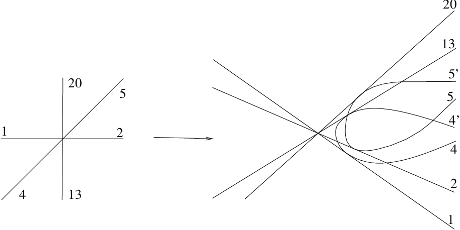
Let us understand how the regeneration of a $6$ -point occurs, by focusing for example on a neighbourhood around $2$ in $S_{0}$ . The first regeneration consists in smoothing out the lines $4$ and $5$ and therefore replacing four of these pairwise adjacent but opposite planes with two quadrics, see Figure 4.

Then one smooths out the lines $13$ and $20$ . This produces two cubic rational normal scrolls meeting along the lines $1$ and $2$ . Now the union of these lines on each scroll is homologous to a non singular conic, so we can further regenerate to make the two scrolls meet along a smooth conic (in this way $1$ and $2$ are replaced by a smooth double conic). We visualize a purely local figure (Figure 5), in order to understand this step.

Finally one smooths the conic too and arrives to a Del-Pezzo sextic in ${\mathbb{C}}{\mathbb{P}}^{6}$ .

A similar regeneration occurs in the neighbourhoods of the other $6$ -points.

5. The braid monodromy factorization $\Delta^{2}_{48}$

In Section 4 we explained how to obtain the branch curve $S$ , which has degree $48$ . At this point we will compute the braid monodromy factorization $\Delta^{2}_{48}$ of $S$ .

In Subsection 5.1 we formulate braids and regeneration rules. In Subsection 5.2 we compute $\Delta^{2}_{48}$ . In Subsections 5.3 and 5.4 we show an invariance property of $\Delta^{2}_{48}$ , and emphasise its importance.

5.1. The regeneration rules

Recall that $Z_{ij}$ is a counterclockwise halftwist of two points $i$ and $j$ . We start with an example that illustrates conjugated braids.

Example 6.

The path on the left-hand side in Figure 6 is constructed as follows: take a path $z_{34}$ and conjugate it by the fulltwist $\bar{Z}_{13}^{2}$ (1 encircles 3 counterclockwise while moving above the axis). We get the left-hand side path $z_{34}^{\bar{Z}_{13}^{2}}$ . The right-hand side path is constructed as follows: take again $z_{34}$ and conjugate it first by $Z_{23}^{2}$ (3 encircles 2 counterclockwise) and then by $Z_{13}^{2}$ (3 encircles 1 counterclockwise while moving below the axis). We get the right-hand side path $z_{34}^{Z_{23}^{2}Z_{13}^{2}}$ . The related halftwists of $z_{34}^{\bar{Z}_{13}^{2}}$ and $z_{34}^{Z_{23}^{2}Z_{13}^{2}}$ are $Z_{34}^{\bar{Z}_{13}^{2}}$ and $Z_{34}^{Z_{23}^{2}Z_{13}^{2}}$ respectively.

In Section 4.2 we explained that by the regeneration one gets the original branch curve $S$ . Let $N,M,u$ be as in Section 3. The set $K=S\cap{\mathbb{C}}_{u}$ are the intersection points of the curve $S$ with the typical fiber ${\mathbb{C}}_{u}$ ; $\#K=48$ . Recall that by the regeneration, each point $c$ in $K_{0}=S_{0}\cap{\mathbb{C}}_{u}$ is replaced by two close points in $K$ , say $c,c^{\prime}$ .

We define the braid $Z^{2}_{ij}$ to be a fulltwist of $j$ around $i$ , and $Z^{2}_{i^{\prime}j}$ to be a fulltwist of $j$ around $i^{\prime}$ . The braid $Z^{2}_{ii^{\prime},j}$ is obtained by a regeneration (the point $i$ on the typical fiber is replaced by $i,i^{\prime}$ ) and it is a fulltwist of $j$ around $i$ and $i^{\prime}$ . This braid (and similar ones) is formulated in the following lemma:

Lemma 7.

[3, Lemma 2.5]
The following formulas hold: $Z^{2}_{ii^{\prime},j}=Z^{2}_{i^{\prime}j}Z^{2}_{ij},\ \ Z^{2}_{i^{\prime},jj^{\prime}}=Z^{2}_{i^{\prime}j^{\prime}}Z^{2}_{i^{\prime}j},\ \ Z^{-2}_{i^{\prime},jj^{\prime}}=Z^{-2}_{i^{\prime}j}Z^{-2}_{i^{\prime}j^{\prime}},\ \ {\bar{Z}}^{-2}_{i^{\prime},jj^{\prime}}={\bar{Z}}^{-2}_{i^{\prime}j^{\prime}}{\bar{Z}}^{-2}_{i^{\prime}j},\ \ Z^{-2}_{ii^{\prime},j}=Z^{-2}_{ij}Z^{-2}_{i^{\prime}j},\ \ Z^{2}_{ii^{\prime},jj^{\prime}}=Z^{2}_{i^{\prime},jj^{\prime}}Z^{2}_{i,jj^{\prime}},\ \ Z^{-2}_{ii^{\prime},jj^{\prime}}=Z^{-2}_{i,jj^{\prime}}Z^{-2}_{i^{\prime},jj^{\prime}}$ .

In the following regeneration rules we shall describe what happens to a factor in a factorized expression of a braid monodromy by a regeneration.

Theorem 8.

First regeneration rule [18, p. 336]
A factor of the form $Z_{ij}$ regenerates to $Z_{ij^{\prime}}Z_{i^{\prime}j}$ .

Theorem 9.

Second regeneration rule [18, p. 337]
A factor of the form $Z^{2}_{ij}$ regenerates to $Z^{2}_{ii^{\prime},j},Z^{2}_{i,jj^{\prime}}$ or $Z^{2}_{ii^{\prime},jj^{\prime}}$ .

Theorem 10.

Third regeneration rule [18, p. 337]
A factor of the form $Z^{4}_{ij}$ regenerates to $Z^{3}_{i,jj^{\prime}}=(Z^{3}_{ij})^{Z_{jj^{\prime}}}\cdot(Z^{3}_{ij})\cdot(Z^{3}_{ij})^{{Z_{jj^{\prime}}}^{-1}}$ or to $Z^{3}_{ii^{\prime},j}=(Z^{3}_{ij})^{Z_{ii^{\prime}}}\cdot(Z^{3}_{ij})\cdot(Z^{3}_{ij})^{{Z_{ii^{\prime}}}^{-1}}$ .

5.2. The factorization

The braid monodromy factorization $\Delta^{2}_{48}$ of $S$ is $\prod\limits^{10}_{i=1}C_{i}\varphi_{i}$ , where $C_{i}$ are the regenerations of the parasitic intersection braids from Section 4.1, and $\varphi_{i}$ are the local braid monodromies which we get when regenerating around the singularities $1,\dots,10$ .

5.2.1. Braid monodromies related to $3$ -points

The $3$ -points are $1,3,6,8$ . We concentrate in the neighbourhood of $1$ , see Figure 3. First the diagonal line $19$ regenerates to a conic $Q_{19}$ which is tangent to the two other lines $1$ and $3$ , see Lemma 5. We compute the braid monodromy $\varphi_{1}$ of the resulting curve.

Proposition 11.

The local braid monodromy $\varphi_{1}$ is

	$\displaystyle\varphi_{1}=$	$\displaystyle Z^{3}_{3\;3^{\prime},19}\cdot{(Z_{1\ 3}\cdot Z_{1\ 3}\cdot Z_{1^{\prime}\ 3}\cdot Z_{1^{\prime}\ 3}\cdot Z_{1\ 3^{\prime}}\cdot Z_{1\ 3^{\prime}}\cdot Z_{1^{\prime}\ 3^{\prime}}\cdot Z_{1^{\prime}\ 3^{\prime}})}^{Z^{2}_{3\;3^{\prime},19}}\cdot$
		$\displaystyle{Z}^{3}_{1\;1^{\prime},19}\cdot{Z_{19\ 19^{\prime}}}^{Z^{2}_{3\;3^{\prime},19}{Z}^{2}_{1\;1^{\prime},19}}.$

Proof.

We follow Figure 3. Let $\pi_{1}:E\times D\rightarrow E$ be the projection to $E$ .

Let $\{j\}^{4}_{j=1}$ be singular points of $\pi_{1}$ as follows: $1$ , $3$ are the tangent points of $Q_{19}$ with the lines $L_{3}$ , $L_{1}$ respectively, $2$ is the intersection point of the lines $L_{1}$ , $L_{3}$ , and $4$ is the branch point in $Q_{19}$ .

Let $N=\{x(j)=x_{j}\mid 1\leq j\leq 4\}$ , such that $N\subset E-\partial E,N\subset E$ . Take $u\in\partial E$ , such that ${\mathbb{C}}_{u}$ is a typical fiber and $M\in{\mathbb{C}}_{u}$ is a real point. Recall that $K=K(M)$ . $K=\{1,3,19,19^{\prime}\}$ , such that the points are real and $1<3<19<19^{\prime}$ . Let $i=L_{i}\cap K$ for $i=1,3$ and $\{19,19^{\prime}\}=Q_{19}\cap K$ .

We are looking for $\varphi_{M}(\delta_{j})$ for $j=1,\ldots,4$ . So we choose a $g$ -base $\{\delta_{j}\}^{4}_{j=1}$ of $\pi_{1}(E-N,u)$ , such that each $\delta_{j}$ is constructed from a path $\gamma_{j}$ below the real line and a counterclockwise small circle around the points in $N$ .

The diffeomorphism which is induced from passing through a branch point was defined in [3] and [15] by $\Delta^{\frac{1}{2}}_{I_{2}{\mathbb{R}}}<k>$ . We recall the precise definition from [3]. Consider a typical fiber on the left side of a branch point (locally defined by $y^{2}-x=0$ ). The typical fiber intersects the conic in two complex points. Passing through this point, these points become real on the right-hand side typical fiber. The two points move to the k’th place and rotate in a counterclockwise $90^{o}$ twist. They become real and numbered as $k,k+1$ .

First find the skeleton $\xi_{x^{\prime}_{j}}$ related to each singular point, as explained in Section 3. Then compute the local diffeomorphisms $\delta_{j}$ induced from singular points $j$ . Since the points $1$ and $3$ (resp. $2$ ) are tangent points (resp. a node), the diffeomorphisms $\delta_{1}$ and $\delta_{3}$ are each of degree $2$ (resp. $1$ ).

$j$	$\xi_{x^{\prime}_{j}}$	$\epsilon_{j}$	$\delta_{j}$
1	$<3,19>$	4	$\Delta^{2}<3,19>$
2	$<1,3>$	2	$\Delta<1,3>$
3	$<3,19>$	4	$\Delta^{2}<3,19>$
4	$<19,19^{\prime}>$	1	$\Delta^{\frac{1}{2}}_{I_{2}{\mathbb{R}}}<19>$

Using [3, Theorems 1.41, 1.44] and [15], we compute the skeleton $(\xi_{x^{\prime}_{j}})\Psi_{\gamma^{\prime}_{j}}$ to each $j$ by applying to the skeleton $\xi_{x^{\prime}_{j}}$ the product $\prod\limits_{i=j-1}^{1}\delta_{i}$ .

$(\xi_{x^{\prime}_{1}})\Psi_{\gamma^{\prime}_{1}}=<3,19>=z_{3\ 19}$
$\varphi_{M}(\delta_{1})=Z^{4}_{3\ 19}$
$(\xi_{x^{\prime}_{2}})\Psi_{\gamma^{\prime}_{2}}=<1,3>\Delta^{2}<3,19>=z_{1\ 3}^{Z^{2}_{3\ 19}}$
$\varphi_{M}(\delta_{2})={Z^{2}_{1\ 3}}^{Z^{2}_{3\ 19}}$
$(\xi_{x^{\prime}_{3}})\Psi_{\gamma^{\prime}_{3}}=<3,19>\Delta<1,3>\Delta^{2}<3,19>={z}_{1\ 19}$
$\varphi_{M}(\delta_{3})={Z}^{4}_{1\ 19}$
$(\xi_{x^{\prime}_{4}})\Psi_{\gamma^{\prime}_{4}}=<19,19^{\prime}>\Delta^{2}<3,19>\Delta<1,3>\Delta^{2}<3,19>=z_{19\ 19^{\prime}}^{Z^{2}_{3\ 19}{Z}^{2}_{1\ 19}}$
$\varphi_{M}(\delta_{4})={Z_{19\ 19^{\prime}}}^{Z^{2}_{3\ 19}{Z}^{2}_{1\ 19}}$

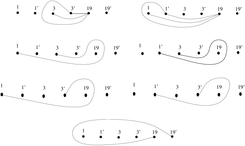
Now, by Theorem 10, in the regeneration process each one of the tangent points regenerates to three cusps. Therefore, the factors $Z^{4}_{3\ 19}$ and ${Z}^{4}_{1\ 19}$ regenerate to $Z^{3}_{3\;3^{\prime},19}$ and ${Z}^{3}_{1\;1^{\prime},19}$ respectively. As explained in Subsection 4.2.1, the node is replaced by eight branch points: since the lines $1$ and $3$ double to be $1$ , $1^{\prime}$ and $3$ , $3^{\prime}$ respectively, we get four nodes, the intersections of $1$ and $3$ , $1^{\prime}$ and $3$ , $1$ and $3^{\prime}$ , $1^{\prime}$ and $3^{\prime}$ . Each node regenerates to two branch points. For $1$ and $3$ we get easily the braid monodromy $Z_{1\ 3}\cdot Z_{1\ 3}$ . For the other ones we get $Z_{1^{\prime}\ 3}\cdot Z_{1^{\prime}\ 3}$ , $Z_{1\ 3^{\prime}}\cdot Z_{1\ 3^{\prime}}$ and $Z_{1^{\prime}\ 3^{\prime}}\cdot Z_{1^{\prime}\ 3^{\prime}}$ . In Figure 7 we show the paths which are related to the braids in $\varphi_{1}$ .

∎

The computations for the points $3,6$ and $8$ are the same. One has to exchange the indices $1,3$ and $19$ to $2,6$ and $14$ (for the point $3$ ), to $7,10$ and $17$ (for the point $6$ ) and to $11,12$ and $24$ (for the point $8$ ) respectively. Therefore we can formulate their related monodromies.

Theorem 12.

The local braid monodromy around the $3$ -point $m=1,3,6$ or $8$ is formulated as follows:

\displaystyle{}\varphi_{m}=

\displaystyle Z^{3}_{j\;j^{\prime},k}\cdot{(Z_{i\ j}\cdot Z_{i\ j}\cdot Z_{i^{\prime}\ j}\cdot Z_{i^{\prime}\ j}\cdot Z_{i\ j^{\prime}}\cdot Z_{i\ j^{\prime}}\cdot Z_{i^{\prime}\ j^{\prime}}\cdot Z_{i^{\prime}\ j^{\prime}})}^{Z^{2}_{j\;j^{\prime},k}}\cdot{Z}^{3}_{i\;i^{\prime},k}\cdot{Z_{k\ k^{\prime}}}^{Z^{2}_{j\;j^{\prime},k}Z^{2}_{i\;i^{\prime},k}},

where $i,j$ and $k$ are the three lines which meet at the $3$ -point $m$ and satisfy $i<j<k$ .

5.2.2. Braid monodromies related to $6$ -points

The $6$ -points in $S_{0}$ are $2,4,5,7,9,10$ . In Section 4.2.2 we recalled the regeneration near the $6$ -point $2$ . The regenerations near $4,5,7,9,10$ are similar to the one around $2$ , but they differ in the indices.

Regenerations in the neighbourhood of a $6$ -points were studied carefully in [3], [5], [6] and [18]. Therefore, we only state the resulting monodromies.

Theorem 13.

The local braid monodromy $\varphi_{2}$ has the following form

	$\displaystyle\varphi_{2}=$	$\displaystyle Z^{2}_{2\;2^{\prime},4}\cdot Z^{2}_{4^{\prime},5\;5^{\prime}}\cdot Z^{3}_{1\;1^{\prime},4}\cdot{Z^{3}_{4^{\prime},13\;13^{\prime}}}^{Z^{2}_{4^{\prime},5\;5^{\prime}}}\cdot{Z^{2}_{2\;2^{\prime},4}}^{Z^{2}_{1\;1^{\prime},4}}\cdot{Z^{2}_{4^{\prime},5\;5^{\prime}}}^{Z^{-2}_{5\;5^{\prime},13\;13^{\prime}}}\cdot$
		$\displaystyle{Z_{4\;4^{\prime}}}^{Z^{2}_{4^{\prime},13\;13^{\prime}}Z^{2}_{4^{\prime},5\;5^{\prime}}Z^{2}_{2\;2^{\prime},4}Z^{2}_{1\;1^{\prime},4}}\cdot{Z^{2}_{4^{\prime},20\;20^{\prime}}}^{Z^{2}_{4^{\prime},13\;13^{\prime}}Z^{2}_{4^{\prime},5\;5^{\prime}}}\cdot$
		$\displaystyle{Z^{2}_{4,20\;20^{\prime}}}^{Z^{2}_{4,13\;13^{\prime}}Z^{2}_{4,5\;5^{\prime}}Z^{2}_{4\;4^{\prime}}Z^{2}_{2\;2^{\prime},4}Z^{2}_{1\;1^{\prime},4}}\cdot\left(G\cdot{\left(F\cdot F^{Z_{20\;20^{\prime}}^{-1}Z_{13\;13^{\prime}}^{-1}}\right)}^{Z^{2}_{2\;2^{\prime},5}Z^{2}_{1\;1^{\prime},5}}\right)^{Z^{2}_{2\;2^{\prime},4}Z^{2}_{1\;1^{\prime},4}},$

where

	$\displaystyle G=$	$\displaystyle Z^{2}_{5^{\prime},13\;13^{\prime}}\cdot Z^{3}_{2\;2^{\prime},5}\cdot{Z^{3}_{5^{\prime},20\;20^{\prime}}}^{Z^{2}_{5^{\prime},13\;13^{\prime}}}\cdot{Z^{2}_{5^{\prime},13\;13^{\prime}}}^{Z^{-2}_{13\;13^{\prime},20\;20^{\prime}}}\cdot{Z_{5\;5^{\prime}}}^{Z^{2}_{2\;2^{\prime},5}Z^{2}_{5^{\prime},20\;20^{\prime}}Z^{2}_{5^{\prime},13\;13^{\prime}}}\cdot$
		$\displaystyle Z^{2}_{1\;1^{\prime},5}\cdot{Z^{2}_{1\;1^{\prime},5^{\prime}}}^{Z^{2}_{5^{\prime},20\;20^{\prime}}Z^{2}_{5^{\prime},13\;13^{\prime}}}$

and

F=Z^{3}_{2\;2^{\prime},13}\cdot Z^{2}_{13^{\prime}\;20}\cdot{Z^{2}_{13\;20}}^{Z^{2}_{2\;2^{\prime},13}}\cdot{Z^{3}_{2\;2^{\prime},20}}^{Z^{2}_{2\;2^{\prime},13}}\cdot\tilde{Z}_{1\;2^{\prime}}\cdot\tilde{Z}_{1^{\prime}\;2}.

The figures which correspond to the braids outside $G$ and $F$ are 8-16. The ones which correspond to the factors in $G$ and $F$ are 17-23 and 24-28 respectively.

In the following theorem we give the local braid monodromies $\varphi_{4},\varphi_{5},\varphi_{7},\varphi_{9}$ and $\varphi_{10}$ . Related figures can be easily constructed, using Example 6. We note that $\varphi_{10}$ was computed precisely in [3] and [18] (and related figures can be found there).

Theorem 14.

(1)

The local braid monodromy $\varphi_{4}$ has the following form

	$\displaystyle\varphi_{4}=$	$\displaystyle Z^{2}_{4^{\prime},7\;7^{\prime}}\cdot{Z^{2}_{4^{\prime},8\;8^{\prime}}}^{Z^{2}_{4^{\prime},7\;7^{\prime}}}\cdot Z^{3}_{3\;3^{\prime},4}\cdot{Z^{3}_{4^{\prime},15\;15^{\prime}}}^{Z^{2}_{4^{\prime},8\;8^{\prime}}Z^{2}_{4^{\prime},7\;7^{\prime}}}\cdot{Z^{2}_{4^{\prime},8\;8^{\prime}}}^{Z^{2}_{4^{\prime},7\;7^{\prime}}Z^{-2}_{8\;8^{\prime},15\;15^{\prime}}}\cdot$
		$\displaystyle{Z^{2}_{4^{\prime},7\;7^{\prime}}}^{Z^{-2}_{7\;7^{\prime},8\;8^{\prime}}Z^{-2}_{7\;7^{\prime},15\;15^{\prime}}}\cdot{Z_{4\;4^{\prime}}}^{Z^{2}_{3\;3^{\prime},4}Z^{2}_{4^{\prime},15\;15^{\prime}}Z^{2}_{4^{\prime},8\;8^{\prime}}Z^{2}_{4^{\prime},7\;7^{\prime}}}\cdot{Z^{2}_{4,21\;21^{\prime}}}^{Z^{2}_{4,15\;15^{\prime}}Z^{2}_{4,8\;8^{\prime}}Z^{2}_{4,7\;7^{\prime}}Z^{2}_{4\;4^{\prime}}Z^{2}_{3\;3^{\prime},4}}\cdot$
		$\displaystyle{Z^{2}_{4^{\prime},21\;21^{\prime}}}^{Z^{2}_{4^{\prime},15\;15^{\prime}}Z^{2}_{4^{\prime},8\;8^{\prime}}Z^{2}_{4^{\prime},7\;7^{\prime}}}\cdot\left(G\cdot{\left(F\cdot F^{Z_{7\;7^{\prime}}^{-1}Z_{3\;3^{\prime}}^{-1}}\right)}^{Z^{2}_{7\;7^{\prime},8}Z^{2}_{3\;3^{\prime},8}}\right)^{Z^{2}_{3\;3^{\prime},4}},$

where

	$\displaystyle G=$	$\displaystyle Z^{2}_{8^{\prime},15\;15^{\prime}}\cdot Z^{3}_{7\;7^{\prime},8}\cdot{Z^{3}_{8^{\prime},21\;21^{\prime}}}^{Z^{2}_{8^{\prime},15\;15^{\prime}}}\cdot{Z^{2}_{8^{\prime},15\;15^{\prime}}}^{Z^{-2}_{15\;15^{\prime},21\;21^{\prime}}}\cdot{Z_{8\;8^{\prime}}}^{Z^{2}_{7\;7^{\prime},8}Z^{2}_{8^{\prime},21\;21^{\prime}}Z^{2}_{8^{\prime},15\;15^{\prime}}}\cdot$
		$\displaystyle Z^{2}_{3\;3^{\prime},8}\cdot{Z^{2}_{3\;3^{\prime},8^{\prime}}}^{Z^{2}_{8^{\prime},21\;21^{\prime}}Z^{2}_{8^{\prime},15\;15^{\prime}}}$

and

F=Z^{2}_{3^{\prime}\;7}\cdot Z^{3}_{7^{\prime},15\;15^{\prime}}\cdot{Z^{2}_{3^{\prime}\;7^{\prime}}}^{Z^{2}_{7^{\prime},15\;15^{\prime}}Z^{2}_{3^{\prime}\;7}}\cdot{Z^{3}_{3^{\prime},15\;15^{\prime}}}^{Z^{2}_{3^{\prime}\;7}}\;\cdot{\tilde{Z}_{15\;21^{\prime}}}\cdot{\tilde{Z}_{15^{\prime}\;21}}.

The paths related to ${\tilde{Z}_{15\;21^{\prime}}}$ and ${\tilde{Z}_{15^{\prime}\;21}}$ appear in Figure 29.

(2)

The local braid monodromy $\varphi_{5}$ has the following form

	$\displaystyle\varphi_{5}=$	$\displaystyle Z^{3}_{5^{\prime},6\;6^{\prime}}\cdot G^{Z^{2}_{5^{\prime},6\;6^{\prime}}}\cdot{Z^{3}_{5^{\prime},22\;22^{\prime}}}^{Z^{2}_{5^{\prime},6\;6^{\prime}}}\cdot{Z_{5\;5^{\prime}}}^{Z^{2}_{5^{\prime},22\;22^{\prime}}Z^{2}_{5^{\prime},6\;6^{\prime}}}\cdot{Z^{2}_{5^{\prime},16\;16^{\prime}}}^{Z^{2}_{5\;5^{\prime}}Z^{2}_{5^{\prime},6\;6^{\prime}}}\cdot$
		$\displaystyle{Z^{2}_{5^{\prime},16\;16^{\prime}}}^{Z^{2}_{5^{\prime},6\;6^{\prime}}}\cdot{Z^{2}_{5,11\;11^{\prime}}}^{Z^{2}_{5\;5^{\prime}}Z^{2}_{5^{\prime},6\;6^{\prime}}}\cdot{Z^{2}_{5^{\prime},11\;11^{\prime}}}^{Z^{2}_{5^{\prime},6\;6^{\prime}}}\cdot{Z^{2}_{5,9\;9^{\prime}}}^{Z^{2}_{5\;5^{\prime}}Z^{2}_{5^{\prime},6\;6^{\prime}}}\cdot{Z^{2}_{5^{\prime},9\;9^{\prime}}}^{Z^{2}_{5^{\prime},6\;6^{\prime}}},$

where

	$\displaystyle G=$	$\displaystyle Z^{2}_{6\;6^{\prime},9}\cdot Z^{3}_{9^{\prime},11\;11^{\prime}}\cdot{Z^{2}_{6\;6^{\prime},9^{\prime}}}^{Z^{2}_{6\;6^{\prime},9}Z^{2}_{9^{\prime},11\;11^{\prime}}}\cdot{\left(F\cdot F^{Z_{11\;11^{\prime}}^{-1}Z_{6\;6^{\prime}}^{-1}}\right)}^{Z^{2}_{6\;6^{\prime},9\;9^{\prime}}Z^{2}_{9^{\prime},11\;11^{\prime}}}\cdot$
		$\displaystyle{Z^{2}_{9^{\prime},22\;22^{\prime}}}^{Z^{2}_{9^{\prime},11\;11^{\prime}}}\cdot Z^{2}_{9,22\;22^{\prime}}\cdot{Z^{3}_{9^{\prime},16\;16^{\prime}}}^{Z^{2}_{9^{\prime},11\;11^{\prime}}}\cdot{Z_{9\;9^{\prime}}}^{Z^{2}_{9^{\prime},16\;16^{\prime}}Z^{2}_{9^{\prime},11\;11^{\prime}}}$

and

F=Z^{2}_{6^{\prime}\;11}\cdot Z^{3}_{11^{\prime},16\;16^{\prime}}\cdot{Z^{2}_{6^{\prime}\;11^{\prime}}}^{Z^{2}_{11^{\prime},16\;16^{\prime}}Z^{2}_{6^{\prime}\;11}}\cdot{Z^{3}_{6^{\prime},16\;16^{\prime}}}^{Z^{2}_{6^{\prime}\;11}}\cdot\tilde{Z}_{16\;22^{\prime}}\cdot\tilde{Z}_{16^{\prime}\;22}.

The paths related to $\tilde{Z}_{16\;22^{\prime}}$ and $\tilde{Z}_{16^{\prime}\;22}$ are the same ones as in Figure 29, with the following exchange of indices: $3\mapsto 6,7\mapsto 11,15\mapsto 16,21\mapsto 22$ .

(3)

The local braid monodromy $\varphi_{7}$ has the following form

	$\displaystyle\varphi_{7}=$	$\displaystyle Z^{2}_{8\;8^{\prime},9}\cdot Z^{2}_{9^{\prime},10\;10^{\prime}}\cdot{Z^{3}_{9^{\prime},12\;12^{\prime}}}^{Z^{2}_{9^{\prime},10\;10^{\prime}}}\cdot{Z^{2}_{9^{\prime},10\;10^{\prime}}}^{Z^{-2}_{10\;10^{\prime},12\;12^{\prime}}}\cdot{Z^{2}_{8\;8^{\prime},9^{\prime}}}^{Z^{2}_{9^{\prime},12\;12^{\prime}}Z^{2}_{9^{\prime},10\;10^{\prime}}Z^{2}_{8\;8^{\prime},9}}\cdot$
		$\displaystyle G^{Z^{2}_{8\;8^{\prime},9\;9^{\prime}}Z^{2}_{9^{\prime},12\;12^{\prime}}Z^{2}_{9^{\prime},10\;10^{\prime}}}\cdot{Z^{2}_{9^{\prime},23\;23^{\prime}}}^{Z^{2}_{9^{\prime},12\;12^{\prime}}Z^{2}_{9^{\prime},10\;10^{\prime}}}\cdot{Z^{3}_{9^{\prime},18\;18^{\prime}}}^{Z^{2}_{9^{\prime},12\;12^{\prime}}Z^{2}_{9^{\prime},10\;10^{\prime}}}\cdot Z^{2}_{9,23\;23^{\prime}}\cdot$
		$\displaystyle{Z_{9\;9^{\prime}}}^{Z^{2}_{9^{\prime},18\;18^{\prime}}Z^{2}_{9^{\prime},12\;12^{\prime}}Z^{2}_{9^{\prime},10\;10^{\prime}}},$

where

	$\displaystyle G=$	$\displaystyle Z^{3}_{8^{\prime},10\;10^{\prime}}\cdot{\left(F\cdot F^{Z_{23\;23^{\prime}}^{-1}Z_{18\;18^{\prime}}^{-1}}\right)}^{Z^{2}_{8^{\prime},10\;10^{\prime}}}\cdot{Z^{3}_{8^{\prime},23\;23^{\prime}}}^{Z^{2}_{8^{\prime},10\;10^{\prime}}}\cdot{Z_{8\;8^{\prime}}}^{Z^{2}_{8^{\prime},23\;23^{\prime}}Z^{2}_{8^{\prime},10\;10^{\prime}}}\cdot$
		$\displaystyle{Z^{2}_{8^{\prime},18\;18^{\prime}}}^{Z^{2}_{8^{\prime},10\;10^{\prime}}}\cdot{Z^{2}_{8,18\;18^{\prime}}}^{Z^{2}_{8\;8^{\prime}}Z^{2}_{8^{\prime},10\;10^{\prime}}}\cdot{Z^{2}_{8^{\prime},12\;12^{\prime}}}^{Z^{2}_{8^{\prime},10\;10^{\prime}}}\cdot{Z^{2}_{8,12\;12^{\prime}}}^{Z^{2}_{8\;8^{\prime}}Z^{2}_{8^{\prime},10\;10^{\prime}}}$

and

F=Z^{3}_{12\;12^{\prime},18}\cdot Z^{2}_{18^{\prime}\;23}\cdot{Z^{2}_{18\;23}}^{Z^{2}_{12\;12^{\prime},18}}\cdot{Z^{3}_{12\;12^{\prime},23}}^{Z^{2}_{12\;12^{\prime},18}}\cdot\tilde{Z}_{10\;12^{\prime}}\cdot\tilde{Z}_{10^{\prime}\;12}.

Moreover, the paths related to $\tilde{Z}_{10\;12^{\prime}}$ and $\tilde{Z}_{10^{\prime}\;12}$ are the same ones as in Figure 28, with the following exchange of indices: $1\mapsto 10,2\mapsto 12,13\mapsto 18,20\mapsto 23$ .

(4)

The local braid monodromy $\varphi_{9}$ has the following form

	$\displaystyle\varphi_{9}=$	$\displaystyle Z^{2}_{14^{\prime},15\;15^{\prime}}\cdot Z^{3}_{13\;13^{\prime},14}\cdot{\bar{Z}}^{3}_{14^{\prime},16\;16^{\prime}}\cdot{Z^{2}_{14^{\prime},15\;15^{\prime}}}^{Z^{-2}_{15\;15^{\prime},16\;16^{\prime}}}\cdot{Z_{14\;14^{\prime}}}^{Z^{2}_{13\;13^{\prime},14}Z^{2}_{14^{\prime},16\;16^{\prime}}Z^{2}_{14^{\prime},15\;15^{\prime}}}\cdot$
		$\displaystyle\left({\bar{Z}}^{2}_{14,17\;17^{\prime}}\right)^{Z^{2}_{13\;13^{\prime},14}}\cdot{\bar{Z}}^{2}_{14^{\prime},17\;17^{\prime}}\cdot\left({\bar{Z}^{2}}_{14,18\;18^{\prime}}\right)^{Z^{2}_{13\;13^{\prime},14}}\cdot{\bar{Z}}^{2}_{14^{\prime},18\;18^{\prime}}\cdot$
		$\displaystyle\left(G\cdot{\left(F\cdot F^{Z_{18\;18^{\prime}}^{-1}Z_{13\;13^{\prime}}^{-1}}\right)}^{Z^{-2}_{17,18\;18^{\prime}}}\right)^{Z^{2}_{13\;13^{\prime},14}},$

where

	$\displaystyle G=$	$\displaystyle Z^{2}_{16\;16^{\prime},17}\cdot Z^{3}_{17^{\prime},18\;18^{\prime}}\cdot{Z^{3}_{15\;15^{\prime},17}}\cdot{Z^{2}_{16\;16^{\prime},17}}^{Z^{2}_{15\;15^{\prime},17}}\cdot{Z_{17\;17^{\prime}}}^{Z^{2}_{17^{\prime},18\;18^{\prime}}Z^{2}_{16\;16^{\prime},17}Z^{2}_{15\;15^{\prime},17}}\cdot$
		$\displaystyle Z^{2}_{13\;13^{\prime},17}\cdot{Z^{2}_{13\;13^{\prime},17^{\prime}}}^{Z^{2}_{17^{\prime},18\;18^{\prime}}}$

and

F=Z^{3}_{13^{\prime},15\;15^{\prime}}\cdot Z^{3}_{16\;16^{\prime},18}\cdot\tilde{Z}_{15\;16^{\prime}}\cdot\tilde{Z}_{15^{\prime}\;16}\cdot{Z^{2}_{13^{\prime}\;18}}^{Z^{2}_{13^{\prime},15\;15^{\prime}}}\cdot Z^{2}_{13\;18}.

The paths related to $\tilde{Z}_{15\;16^{\prime}}$ and $\tilde{Z}_{15^{\prime}\;16}$ appear in Figure 30.

(5)

The local braid monodromy $\varphi_{10}$ has the following form

	$\displaystyle\varphi_{10}=$	$\displaystyle Z^{3}_{19^{\prime},20\;20^{\prime}}\cdot{Z_{24\;24^{\prime}}}^{Z_{22\;22^{\prime},24}^{-2}Z_{23\;23^{\prime},24}^{-2}}\cdot Z^{2}_{21\;21^{\prime},24^{\prime}}\cdot{\bar{Z}}^{3}_{22\;22^{\prime},24}\cdot{Z^{2}_{21\;21^{\prime},24}}^{Z^{-2}_{23\;23^{\prime},24}}\cdot$
		$\displaystyle G^{Z^{2}_{19^{\prime},20\;20^{\prime}}}\cdot Z^{3}_{23\;23^{\prime},24}\cdot{\bar{Z}}^{3}_{19^{\prime},21\;21^{\prime}}\cdot Z^{2}_{19,22\;22^{\prime}}\cdot Z^{2}_{19,23\;23^{\prime}}\cdot Z^{2}_{19,24\;24^{\prime}},$

where

	$\displaystyle G=$	$\displaystyle Z^{2}_{20\;20^{\prime},24^{\prime}}\cdot{Z^{2}_{20\;20^{\prime},24}}^{Z^{-2}_{23\;23^{\prime},24}}\cdot\left(F\cdot F^{Z_{23\;23^{\prime}}^{-1}Z_{20\;20^{\prime}}^{-1}}\right)^{Z^{-2}_{23\;23^{\prime},24}}\cdot Z^{2}_{19^{\prime},22\;22^{\prime}}\cdot$
		$\displaystyle Z^{2}_{19^{\prime},23\;23^{\prime}}\cdot Z^{2}_{19^{\prime},24\;24^{\prime}}\cdot{Z_{19\;19^{\prime}}}^{Z^{2}_{19^{\prime},21\;21^{\prime}}}$

and

F=Z^{3}_{20^{\prime},21\;21^{\prime}}\cdot Z^{3}_{22\;22^{\prime},23}\cdot\tilde{Z}_{21\;22^{\prime}}\cdot\tilde{Z}_{21^{\prime}\;22}\cdot{Z^{2}_{20^{\prime}\;23}}^{Z^{2}_{20^{\prime},21\;21^{\prime}}}\cdot Z^{2}_{20\;23}.

The paths related to $\tilde{Z}_{21\;22^{\prime}}$ and $\tilde{Z}_{21^{\prime}\;22}$ are the same ones as in Figure 30, with the following exchange of indices: $13\mapsto 20,15\mapsto 21,16\mapsto 22,18\mapsto 23$ .

5.2.3. The products $C_{i}$

The deformation also regenerates the parasitic intersection braids ${\{{\tilde{C}_{i}}\}}_{i=1}^{10}$ , see Theorem 9. By [18, Lemma 19], we can take the complex conjugations

	$\displaystyle D_{1}=$	$\displaystyle D_{2}=D_{4}=Id\ ,\ D_{3}=Z^{2}_{2\;2^{\prime},3\;3^{\prime}}\ ,\ D_{5}={Z}^{2}_{3\;3^{\prime},5\;5^{\prime}}\ ,\ D_{6}=\prod\limits_{i=1,3,4}\stackrel{{\scriptstyle\scriptstyle(5)(5^{\prime})}}{{Z^{2}}}_{\hskip-11.38092pti\;i^{\prime},6\;6^{\prime}}\ ,$
	$\displaystyle\ D_{7}=$	$\displaystyle\prod\limits_{i=1,2,5,6}{Z^{2}}_{\hskip-5.69046pti\;i^{\prime},7\;7^{\prime}}\ ,\ D_{8}=\prod\limits_{i=1,2,5,6}Z^{2}_{i\;i^{\prime},8\;8^{\prime}}\ ,\ D_{9}=\prod\limits_{i=1-4,7}\stackrel{{\scriptstyle\scriptstyle(8)(8^{\prime})}}{{Z^{2}}}_{\hskip-11.38092pti\;i^{\prime},9\;9^{\prime}}\ ,\ D_{10}=\prod\limits_{i=1}^{6}\stackrel{{\scriptstyle\scriptstyle(8)-(9^{\prime})}}{{Z^{2}}}_{\hskip-11.38092pti\;i^{\prime},10\;10^{\prime}}\ ,$
	$\displaystyle\ D_{11}=$	$\displaystyle\prod\limits_{\stackrel{{\scriptstyle i=1}}{{i\neq 5,6,9}}}^{10}{Z^{2}}_{\hskip-2.84544pti\;i^{\prime},11\;11^{\prime}}\ ,\ D_{12}=\prod\limits^{7}_{i=1}\stackrel{{\scriptstyle\scriptstyle(11)(11^{\prime})}}{{Z^{2}}}_{\hskip-14.22636pti\;i^{\prime},12\;12^{\prime}}\ ,\ D_{13}=\prod\limits^{12}_{\stackrel{{\scriptstyle i=3}}{{i\neq 4,5}}}Z^{2}_{i\;i^{\prime},13\;13^{\prime}}\ ,$
	$\displaystyle\ D_{14}=$	$\displaystyle\prod\limits^{12}_{\stackrel{{\scriptstyle i=1}}{{i\neq 2,6}}}\stackrel{{\scriptstyle\scriptstyle(13)(13^{\prime})}}{{Z^{2}}}_{\hskip-11.38092pti\;i^{\prime},14\;14^{\prime}}\ ,\ D_{15}=\prod\limits^{12}_{\stackrel{{\scriptstyle i=1}}{{i\neq 3,4,7,8}}}\stackrel{{\scriptstyle\scriptstyle(13)-(14^{\prime})}}{{Z^{2}}}_{\hskip-17.07182pti\;i^{\prime},15\;15^{\prime}}\ ,\ D_{16}=\prod\limits^{12}_{\stackrel{{\scriptstyle i=1}}{{i\neq 5,6,9,11}}}\stackrel{{\scriptstyle\scriptstyle(13)-(15^{\prime})}}{{Z^{2}}}_{\hskip-17.07182pti\;i^{\prime},16\;16^{\prime}}\ ,$
	$\displaystyle\ D_{17}=$	$\displaystyle\prod\limits^{12}_{\stackrel{{\scriptstyle i=1}}{{i\neq 7,10}}}\stackrel{{\scriptstyle\scriptstyle(13)-(16^{\prime})}}{{Z^{2}}}_{\hskip-17.07182pti\;i^{\prime},17\;17^{\prime}}\ ,\ D_{18}=\prod\limits^{11}_{\stackrel{{\scriptstyle i=1}}{{i\neq 8-10}}}\stackrel{{\scriptstyle\scriptstyle(13)-(17^{\prime})}}{{Z^{2}}}_{\hskip-17.07182pti\;i^{\prime},18\;18^{\prime}}\ ,\ D_{19}=\prod\limits^{18}_{\stackrel{{\scriptstyle i=2}}{{i\neq 3}}}Z^{2}_{i\;i^{\prime},19\;19^{\prime}}\ ,$
	$\displaystyle\ D_{20}=$	$\displaystyle\prod\limits^{18}_{\stackrel{{\scriptstyle i=3}}{{i\neq 4,5,13}}}\stackrel{{\scriptstyle\scriptstyle(19)(19^{\prime})}}{{Z^{2}}}_{\hskip-11.38092pti\;i^{\prime},20\;20^{\prime}}\ ,\ D_{21}=\prod\limits^{18}_{\stackrel{{\scriptstyle i=1}}{{i\neq 3,4,7,8,15}}}\stackrel{{\scriptstyle\scriptstyle(19)-(20^{\prime})}}{{Z^{2}}}_{\hskip-17.07182pti\;i^{\prime},21\;21^{\prime}}\ ,\ D_{22}=\prod\limits^{18}_{\stackrel{{\scriptstyle i=1}}{{i\neq 5,6,9,11,16}}}\stackrel{{\scriptstyle\scriptstyle(19)-(21^{\prime})}}{{Z^{2}}}_{\hskip-17.07182pti\;i^{\prime},22\;22^{\prime}}\ ,$
	$\displaystyle\ D_{23}=$	$\displaystyle\prod\limits^{17}_{\stackrel{{\scriptstyle i=1}}{{i\neq 8-10,12}}}\stackrel{{\scriptstyle\scriptstyle(19)-(22^{\prime})}}{{Z^{2}}}_{\hskip-17.07182pti\;i^{\prime},23\;23^{\prime}}\ ,\ D_{24}=\prod\limits^{18}_{\stackrel{{\scriptstyle i=1}}{{i\neq 11,12}}}\stackrel{{\scriptstyle\scriptstyle(19)-(23^{\prime})}}{{Z^{2}}}_{\hskip-17.07182pti\;i^{\prime},24\;24^{\prime}}.$

Let us denote the regenerations of $\tilde{C}_{i}$ as $C_{i}$ , $1\leq i\leq 10$ . These are the factorizations of the suitable $D_{t}$ , as in (1).

5.3. Properties of the factorization $\Delta_{48}^{2}$

The braid monodromy factorization $\Delta_{48}^{2}$ is the product $\prod\limits_{i=1}^{10}C_{i}\varphi_{i}$ . We now verify that there are no missing braids.

Proposition 15.

The braid monodromy factorization of $S$ is $\Delta_{48}^{2}$ .

Proof.

By Proposition V.2.2 in [14], deg $\Delta_{48}^{2}=48\cdot 47=2256$ .

Now we check the degree of the factorization $\prod\limits_{i=1}^{10}C_{i}\varphi_{i}$ . The monodromies ${\{{\varphi_{i}}\}}_{i=1,3,6,8}$ each consist of six cusps and nine branch points, see Section 5.2.1. We combine their degrees to get $4\cdot(6\cdot 3+1\cdot 9)=4\cdot 27=108$ .

In each $\varphi_{i},i=2,4,5,7,9,10$ (Section 5.2.2), $\deg F(F)^{*}=48$ . The factors outside $F(F)^{*}$ are $20$ degree two factors, $12$ degree three factors, and $2$ degree one factors. Combining the degrees of these, we get $20\cdot 2+12\cdot 3+2\cdot 1=78$ . Thus $\deg\varphi_{i}=78+48=126$ for $i=2,4,5,7,9,10$ , and therefore $\deg(\prod\limits_{i=2,4,5,7,9,10}\varphi_{i})=126\cdot 6=756$ .

The products ${\{{C_{i}}\}}_{i=1}^{10}$ consist of $696$ nodes, see Section 5.2.3. We combine degrees of their factors to get $\deg\prod\limits_{i=1}^{10}{C_{i}}=696\cdot 2=1392$ .

Finally $\deg\prod\limits^{10}_{i=1}C_{i}\varphi_{i}=108+756+1392=2256$ . Therefore $\Delta_{48}^{2}$ is the desired braid monodromy factorization. ∎

We now study invariance properties of $\Delta^{2}_{48}$ . Invariance properties are results in which we prove that the braid monodromy factorization $\Delta^{2}_{48}$ is invariant under certain elements of $B_{48}$ . Establishing invariance properties is essential in order to simplify the computations which follow from the van Kampen Theorem (see [4]); at the end of this section we describe the effect of these properties on the application of the van Kampen Theorem.

The following definitions are necessary in order to prove the Invariance Properties.

Definition 16.

Let $g_{1}\cdots g_{k}=h_{1}\cdots h_{k}$ be two factorized expressions of the same element in a group $G$ . We say that $g_{1}\cdots g_{k}$ is obtained from $h_{1}\cdots h_{k}$ by a Hurwitz move if $\exists\ 1\leq p\leq k-1$ , such that $g_{i}=h_{i}\ (i\neq p,p+1)\ g_{p}=h_{p}h_{p+1}h^{-1}_{p}$ and $g_{p+1}=h_{p}$ or $g_{p}=h_{p+1}$ and $g_{p+1}=h^{-1}_{p+1}h_{p}h_{p+1}$ . In general, $g_{1}\cdots{g_{k}}\simeq h_{1}\cdots h_{k}$ (Hurwitz equivalent) if $g_{1}\cdots{g_{k}}$ is obtained from $h_{1}\cdots h_{k}$ by a finite number of Hurwitz moves.

Definition 17.

Let $g_{1}\cdots g_{k}$ be a factorized expression in $G$ and $h\in G$ . We say that $g_{1}\cdots g_{k}$ is invariant under $h$ if it is Hurwitz equivalent to $(g_{1})_{h}\cdots(g_{k})_{h}$ , where $(g_{i})_{h}=h^{-1}g_{i}h$ .

Invariance properties are important in view of Lemma VI.4.2 in [14]: if a braid monodromy factorization $\Delta^{2}_{n}$ is invariant under $h$ then the equivalent factorization $(\Delta^{2}_{n})_{h}$ is also a braid monodromy factorization.

We now quote several invariance rules (the conclusions of Theorems 8, 9, 10), Chakiri’s Lemma (see [18]), and make some remarks on invariance properties.

Invariance Rules

(1)

A braid $Z^{1}_{ij}$ is invariant under $(Z_{ii^{\prime}}Z_{jj^{\prime}})^{q}$ for any $q\in{\mathbb{Z}}$ .
(2)

A braid $Z^{2}_{i,jj^{\prime}}$ (resp. $Z^{2}_{ii^{\prime},jj^{\prime}}$ ) is invariant under $Z_{jj^{\prime}}^{q}$ (resp. $Z_{ii^{\prime}}^{p}Z^{q}_{jj^{\prime}}$ ) for any $p,q\in{\mathbb{Z}}$ .
(3)

$Z^{3}_{i,jj^{\prime}}$ is invariant under $Z_{jj^{\prime}}^{q}$ for any $q\in{\mathbb{Z}}$ .

Lemma 18.

(Chakiri). Let $g=g_{1}\cdots g_{k}$ be a factorized expression in a group $G$ . Then $g_{1}\cdots g_{k}$ is invariant under $g^{m}$ for any $m\in{\mathbb{Z}}$ .

Invariance Remarks

(1)

To prove invariance of $g_{1}\cdots g_{k}$ under $h$ it is enough to prove that $g_{1}\cdots g_{t}$ and $g_{t+1}\cdots g_{k}$ are invariant under $h$ . Thus we can divide a factorization into subfactorizations and prove invariance on each part separately.
(2)

An element $g_{1}$ is invariant under $h$ if and only if $g_{1}$ commutes with $h$ .
(3)

If a product of elements that commutes with $h$ is invariant under $h$ , the corresponding factorizations are equal.
(4)

If two paths $\sigma_{1}$ and $\sigma_{2}$ do not intersect, the corresponding halftwists $H(\sigma_{1})$ and $H(\sigma_{2})$ commute.
(5)

If $g$ is invariant under $h_{1}$ and $h_{2}$ then $g$ is invariant under $h_{1}h_{2}$ .

We finally prove the Invariance Properties of $\Delta^{2}_{48}$ . Denote $Z_{ij}=H(z_{ij})$ .

Remark 19.

The halftwists $Z_{ii^{\prime}}$ and $Z_{jj^{\prime}}$ commute for all $i,j$ , since the path from $i$ to $i^{\prime}$ does not intersect the path from $j$ to $j^{\prime}$ .

Lemma 20.

Each monodromy among $\varphi_{1},\varphi_{3},\varphi_{6},\varphi_{8}$ is invariant under $\prod\limits^{24}_{j=1}Z^{m_{j}}_{jj^{\prime}}$ for $m_{j}\in{\mathbb{Z}}$ .

Proof.

The braids in $\varphi_{1},\varphi_{3},\varphi_{6},\varphi_{8}$ , arise from cusps and branch points (see Theorem 12). By Invariance Rule (3), each braid of the form $Z^{3}_{ii^{\prime},j}$ is invariant under $Z_{ii^{\prime}}^{q}$ . Each of the braids of the form $Z^{1}_{ij}$ is invariant under $(Z_{ii^{\prime}}Z_{jj^{\prime}})^{q}$ , and in particular, if the braid is of the form $Z^{1}_{ii^{\prime}}$ , then it is invariant under $Z_{ii^{\prime}}^{q}$ .

Moreover, by Remark 19, each $Z_{kk^{\prime}}$ commutes with the above braids when $k\neq i,j$ .

Therefore, each monodromy $\varphi_{i}$ , $i=1,3,6,8$ , is invariant under $\prod\limits^{24}_{j=1}Z^{m_{j}}_{jj^{\prime}}$ for $m_{j}\in{\mathbb{Z}}$ . ∎

Lemma 21.

Each factorization $\{C_{i}\}$ , $i=1,\dots,10$ , is invariant under $\prod\limits^{24}_{j=1}Z^{m_{j}}_{jj^{\prime}}$ for $m_{j}\in{\mathbb{Z}}$ .

Proof.

We apply Invariance Rule (2) and Invariance Remark (4) to each $C_{i}$ to get the desired invariance. ∎

We now prove invariance for the monodromy $\varphi_{2}$ . A similar proof will apply for each one of the monodromies $\varphi_{4},\varphi_{5},\varphi_{7},\varphi_{9},\varphi_{10}$ .

Lemma 22.

$\varphi_{2}$ is invariant under $(Z_{4\;4^{\prime}}Z_{5^{\prime}\;5^{\prime}})^{p}(Z_{13\;13^{\prime}}Z_{20\;20^{\prime}})^{q}(Z_{1\;1^{\prime}}Z_{2\;2^{\prime}})^{r}$ for all $p,q,r\in{\mathbb{Z}}$ .

Proof.

Case 1: $p=q=r$ .
As proved in [18, Lemma 12], the monodromy $\varphi_{2}$ can be written as $\prod\limits_{j=1,2,4,5,13,20}Z_{jj^{\prime}}^{-1}\Delta_{12}^{2}$ . By Lemma 18, $\varphi_{2}$ is invariant under $(\prod\limits_{j=1,2,4,5,13,20}Z_{jj^{\prime}}^{-1}\Delta_{12}^{2})^{-p}$ . Since $\Delta_{12}^{2}$ is a central element, $\varphi_{2}$ is invariant under $(Z_{4\;4^{\prime}}Z_{5\;5^{\prime}})^{p}(Z_{13\;13^{\prime}}Z_{20\;20^{\prime}})^{p}(Z_{1\;1^{\prime}}Z_{2\;2^{\prime}})^{p}$ .

Case 2: $p=0$ .
Let $\epsilon=(Z_{13\;13^{\prime}}Z_{20\;20^{\prime}})^{q}(Z_{1\;1^{\prime}}Z_{2\;2^{\prime}})^{r}$ .

(1)

Step 1: Factors outside of $F\cdot F^{Z_{20\;20^{\prime}}^{-1}Z_{13\;13^{\prime}}^{-1}}$ .
${Z_{4\;4^{\prime}}}^{Z^{2}_{4^{\prime},13\;13^{\prime}}Z^{2}_{4^{\prime},5\;5^{\prime}}Z^{2}_{2\;2^{\prime},4}Z^{2}_{1\;1^{\prime},4}}$ and ${Z_{5\;5^{\prime}}}^{Z^{2}_{2\;2^{\prime},5}Z^{2}_{5^{\prime},20\;20^{\prime}}Z^{2}_{5^{\prime},13\;13^{\prime}}Z^{2}_{2\;2^{\prime},4}Z^{2}_{1\;1^{\prime},4}}$ commute with $\epsilon$ .
$Z^{3}_{1\;1^{\prime},4},{Z^{3}_{4^{\prime},13\;13^{\prime}}}^{Z^{2}_{4^{\prime},5\;5^{\prime}}},{Z^{3}_{2\;2^{\prime},5}}^{Z^{2}_{2\;2^{\prime},4}Z^{2}_{1\;1^{\prime},4}}$ and ${Z^{3}_{5^{\prime},20\;20^{\prime}}}^{Z^{2}_{5^{\prime},13\;13^{\prime}}Z^{2}_{2\;2^{\prime},4}Z^{2}_{1\;1^{\prime},4}}$ are invariant under $\epsilon$ by Invariance Rule (3).
The degree 2 factors are of the form $Z^{2}_{\alpha\alpha^{\prime},\beta}$ where $\beta=4,4^{\prime},5,5^{\prime}$ . By Invariance Rule (2), they are invariant under $Z_{\alpha\alpha^{\prime}}$ , and since the other halftwists in $\epsilon$ commute with $Z_{\alpha\beta}$ and $Z_{\alpha^{\prime}\beta}$ , we get that $Z^{2}_{\alpha\alpha^{\prime},\beta}$ is invariant under $\epsilon$ .
Moreover all conjugations which appear in $\varphi_{2}$ (i.e. ${(\ \ )}^{*}$ ) are invariant under $\epsilon$ by Invariance Rule (2) and by Invariance Remark (4).

(2)

Step 2: Factors in $F\cdot F^{Z_{20\;20^{\prime}}^{-1}Z_{13\;13^{\prime}}^{-1}}$ .
Let $\rho=Z_{13\;13^{\prime}}Z_{20\;20^{\prime}}$ . In order to prove that $F\cdot F^{\rho^{-1}}$ is invariant under $\epsilon$ , we consider the following subcases:

•

Subcase 2.1: $q=0$ and $\epsilon=(Z_{1\;1^{\prime}}Z_{2\;2^{\prime}})^{r}$ .
$Z^{3}_{2\;2^{\prime},13}$ and ${Z^{3}_{2\;2^{\prime},20}}^{Z^{2}_{2\;2^{\prime},13}}$ are invariant under $Z_{2\;2^{\prime}}$ (Invariance Rule (3)) and commute with $Z_{1\;1^{\prime}}$ (Invariance Remark (4)). Thus $Z^{3}_{2\;2^{\prime},13}{Z^{3}_{2\;2^{\prime},20}}^{Z^{2}_{2\;2^{\prime},13}}$ is invariant under $\epsilon$ (Invariance Remarks (1) and (5)). $Z^{2}_{13^{\prime}\;20}$ and $\cdot(Z^{2}_{13\;20})^{Z^{2}_{2\;2^{\prime},13}}$ commute with $Z_{1\;1^{\prime}}$ and $Z_{2\;2^{\prime}}$ and thus with $\epsilon$ . $\tilde{Z}_{1\;2^{\prime}}\cdot\tilde{Z}_{1^{\prime}\;2}$ is invariant under $(Z_{1\;1^{\prime}}Z_{2\;2^{\prime}})^{r}$ by Invariance Rule (1). For $F^{\rho^{-1}}$ we have the same conclusion, since $Z^{-1}_{20\;20^{\prime}}Z^{-1}_{13\;13^{\prime}}$ commutes with $\epsilon=(Z_{1\;1^{\prime}}Z_{2\;2^{\prime}})^{r}$ .

•

Subcase 2.2: $r=0\ ,\ q=1$ and $\epsilon=Z_{13\;13^{\prime}}Z_{20\;20^{\prime}}$ .
Note that in this case $\epsilon=\rho$ . To prove that $F\cdot F^{\rho^{-1}}$ is invariant under $\rho$ , we must show that $F\cdot F^{\rho^{-1}}$ is Hurwitz equivalent to $F^{\rho}\cdot F$ . Since $AB$ is Hurwitz equivalent to $BA^{B}$ , it is enough to prove that $F\cdot F^{\rho^{-1}}$ is Hurwitz equivalent to $F\cdot{(F^{\rho})}^{F}$ . Thus it is enough to prove that $F^{\rho^{-1}}$ is Hurwitz equivalent to ${(F^{\rho})}^{F}$ or that ${(F^{\rho^{-1}})}^{F^{-1}}$ is Hurwitz equivalent to $F^{\rho}$ .

By Theorem 13, $F=\Delta^{2}_{8}\rho^{-2}Z^{-2}_{1\;1^{\prime}}Z^{-2}_{2\;2^{\prime}}(F^{-1})^{\rho^{-1}}$ , thus $F^{-1}=F^{\rho^{-1}}(Z_{1\;1^{\prime}}Z_{2\;2^{\prime}})^{2}\rho^{2}\Delta^{2}_{8}$ . Now we have

	$\displaystyle(F^{\rho^{-1}})^{F^{-1}}=(F^{\rho^{-1}})^{F^{\rho^{-1}}(Z_{1\;1^{\prime}}Z_{2\;2^{\prime}})^{2}\rho^{2}\Delta^{2}_{8}}\left.\begin{array}[]{c}=\\[-14.22636pt] {\scriptstyle as\ factorized}\\[-14.22636pt] {\scriptstyle expression}\end{array}\right.(F^{\rho^{-1}})^{F^{\rho^{-1}}(Z_{1\;1^{\prime}}Z_{2\;2^{\prime}})^{2}\rho^{2}}$
	$\displaystyle\left.\begin{array}[]{c}\simeq\\[-14.22636pt] {\scriptstyle Chakiri}\end{array}\right.(F^{\rho^{-1}})^{(Z_{1\;1^{\prime}}Z_{2\;2^{\prime}})^{2}\rho^{2}}={(F^{(Z_{1\;1^{\prime}}Z_{2\;2^{\prime}})^{2}})}^{\rho}\;\left.\begin{array}[]{c}\simeq\\[-14.22636pt] {\scriptstyle\ Subcase\ 2.1}\end{array}\right.F^{\rho}.$

•

Subcase 2.3: $q=2q^{\prime}\ ;\ \epsilon=(Z_{13\;13^{\prime}}Z_{20\;20^{\prime}})^{2q^{\prime}}(Z_{1\;1^{\prime}}Z_{2\;2^{\prime}})^{r}$ .
$F\cdot F^{\rho^{-1}}$ can be written as $\Delta^{2}_{8}(Z_{13\;13^{\prime}}Z_{20\;20^{\prime}})^{-2}(Z_{1\;1^{\prime}}Z_{2\;2^{\prime}})^{-2}$ . By Chakiri’s Lemma, $F\cdot F^{\rho^{-1}}$ is invariant under ${(\Delta^{2}_{8}(Z_{13\;13^{\prime}}Z_{20\;20^{\prime}})^{-2}(Z_{1\;1^{\prime}}Z_{2\;2^{\prime}})^{-2})}^{-q^{\prime}}$ and thus under $(Z_{13\;13^{\prime}}Z_{20\;20^{\prime}})^{2q^{\prime}}(Z_{1\;1^{\prime}}Z_{2\;2^{\prime}})^{2q^{\prime}}$ . By Subcase 2.1, $F\cdot F^{\rho^{-1}}$ is invariant under $(Z_{1\;1^{\prime}}Z_{2\;2^{\prime}})^{r-2q^{\prime}}$ . By Invariance Remark (5), $F\cdot F^{\rho^{-1}}$ is invariant under

(Z_{13\;13^{\prime}}Z_{20\;20^{\prime}})^{2q^{\prime}}(Z_{1\;1^{\prime}}Z_{2\;2^{\prime}})^{2q^{\prime}}(Z_{1\;1^{\prime}}Z_{2\;2^{\prime}})^{r-2q^{\prime}}=\epsilon.

•

Subcase 2.4: $q=2q^{\prime}+1\ ;\ \epsilon=(Z_{13\;13^{\prime}}Z_{20\;20^{\prime}})^{2q^{\prime}+1}(Z_{1\;1^{\prime}}Z_{2\;2^{\prime}})^{r}$ .
It is easy to verify this case by using the prior cases 2.2, 2.3 and Invariance Remark (5).

Case 3: $p,q,r$ arbitrary; $\epsilon=(Z_{4\;4^{\prime}}Z_{5\;5^{\prime}})^{p}(Z_{13\;13^{\prime}}Z_{20\;20^{\prime}})^{q}(Z_{1\;1^{\prime}}Z_{2\;2^{\prime}})^{r}$ .
By case 1, $\varphi_{2}$ is invariant under $(Z_{4\;4^{\prime}}Z_{5\;5^{\prime}})^{p}(Z_{13\;13^{\prime}}Z_{20\;20^{\prime}})^{p}(Z_{1\;1^{\prime}}Z_{2\;2^{\prime}})^{p}$ , and by case 2 under $(Z_{13\;13^{\prime}}Z_{20\;20^{\prime}})^{q-p}(Z_{1\;1^{\prime}}Z_{2\;2^{\prime}})^{r-p}$ . By Invariance Remark (5), $\varphi_{2}$ is invariant under $\epsilon$ . ∎

Corollary 23.

Each one of the monodromies $\varphi_{4},\varphi_{5},\varphi_{7},\varphi_{9},\varphi_{10}$ is invariant under
$(Z_{ii^{\prime}}Z_{jj^{\prime}})^{p}(Z_{kk^{\prime}}Z_{ll^{\prime}})^{q}(Z_{mm^{\prime}}Z_{nn^{\prime}})^{r}$ for all $p,q,r\in{\mathbb{Z}}$ , where $i$ and $j$ are the diagonal lines around the relevant $6$ -point, and $k$ and $l$ (resp. $m$ and $n$ ) are the vertical (resp. horizontal) ones (see Figure 1).

Since the proof of the invariance for the $6$ -points relies on the invariance of each local braid monodromy under such expressions as in Corollary 23, we have to pay attention that each diagonal line (except the lines 14, 17, 19, 24 in Figure 1) at a certain $6$ -point is also a diagonal line at another $6$ -point. For example, the monodromy $\varphi_{2}$ is invariant under $(Z_{4\;4^{\prime}}Z_{5\;5^{\prime}})^{p}(Z_{13\;13^{\prime}}Z_{20\;20^{\prime}})^{q}(Z_{1\;1^{\prime}}Z_{2\;2^{\prime}})^{r}$ for all $p,q,r\in{\mathbb{Z}}$ (see Lemma 22). In addition, the monodromy $\varphi_{4}$ is invariant under $(Z_{4\;4^{\prime}}Z_{8\;8^{\prime}})^{p^{\prime}}(Z_{3\;3^{\prime}}Z_{7\;7^{\prime}})^{q^{\prime}}(Z_{15\;15^{\prime}}Z_{21\;21^{\prime}})^{r^{\prime}}$ for all $p^{\prime},q^{\prime},r^{\prime}\in{\mathbb{Z}}$ (see Corollary 23). This implies that $p=p^{\prime}$ . In the same way, $\varphi_{5}$ is invariant under $(Z_{5\;5^{\prime}}Z_{9\;9^{\prime}})^{p^{\prime\prime}}(Z_{6\;6^{\prime}}Z_{11\;11^{\prime}})^{q^{\prime\prime}}(Z_{16\;16^{\prime}}Z_{22\;22^{\prime}})^{r^{\prime\prime}}$ for all $p^{\prime\prime},q^{\prime\prime},r^{\prime\prime}\in{\mathbb{Z}}$ . This implies that $p=p^{\prime\prime}$ . In the notation of Lemmas 20 and 21, $p=m_{4}=m_{5},p^{\prime}=m_{4}=m_{8},p^{\prime\prime}=m_{5}=m_{9}$ , and therefore $m_{4}=m_{5}=m_{8}=m_{9}$ . Now, the lines 14 and 17 (resp. 19 and 24) are diagonal lines at only one $6$ -point 9 (resp. 10). Therefore in the above notation, $m_{14}=m_{17}$ (resp. $m_{19}=m_{24}$ ).

We now consider the vertical lines. By a similar argument as above, we can conclude that $m_{13}=m_{18}=m_{20}=m_{23}$ from the invariance of $\varphi_{2},\varphi_{7},\varphi_{9}$ and $\varphi_{10}$ . Since the lines $6$ and $11$ (resp. $3$ and $7$ ) are vertical lines at only one $6$ -point 5 (resp. 4), we get $m_{6}=m_{11}$ (resp. $m_{3}=m_{7}$ ).

For the horizontal lines, we can immediately conclude that $m_{1}=m_{2},m_{10}=m_{12}$ , and $m_{15}=m_{16}=m_{21}=m_{22}$ .

Corollary 24.

The braid monodromy factorization $\Delta_{48}^{2}$ is invariant under

	$\displaystyle\rho=$	$\displaystyle{(Z_{1\;1^{\prime}}Z_{2\;2^{\prime}})}^{m_{1}}{(Z_{6\;6^{\prime}}Z_{11\;11^{\prime}})}^{m_{6}}{(Z_{10\;10^{\prime}}Z_{12\;12^{\prime}})}^{m_{10}}{(Z_{3\;3^{\prime}}Z_{7\;7^{\prime}})}^{m_{3}}{(Z_{14\;14^{\prime}}Z_{17\;17^{\prime}})}^{m_{14}}{(Z_{19\;19^{\prime}}Z_{24\;24^{\prime}})}^{m_{19}}$
		$\displaystyle{(Z_{4\;4^{\prime}}Z_{5\;5^{\prime}}Z_{8\;8^{\prime}}Z_{9\;9^{\prime}})}^{m_{4}}{(Z_{13\;13^{\prime}}Z_{18\;18^{\prime}}Z_{20\;20^{\prime}}Z_{23\;23^{\prime}})}^{m_{13}}{(Z_{15\;15^{\prime}}Z_{16\;16^{\prime}}Z_{21\;21^{\prime}}Z_{22\;22^{\prime}})}^{m_{15}}.$

5.4. Consequences from the Invariance Theorems

We are interested in the fundamental group $\pi_{1}({\mathbb{C}}{\mathbb{P}}^{2}-S)$ and the fundamental group of the Galois cover of the surface (with respect to the generic projection onto ${\mathbb{C}}{\mathbb{P}}^{2}$ ). These groups are computed in [4].

Here we extract qualitative information concerning the importance of the above computations and how they are connected to the groups.

The van Kampen Theorem [20] induces a finite presentation of the fundamental group of complements of curves by means of generators and relations. This is done by applying the theorem on the resulting factorization $\Delta^{2}_{48}$ . We take any path from $k$ to $\ell$ , cut it in $M$ , then towards $k$ along the path, around $k$ and coming back the same way. Consider $A$ as an element of the fundamental group. Do the same to $\ell$ to obtain $B$ . See Figure 31. Now, according to the van Kampen Theorem we obtain a relation which involves $A$ and $B$ .

The following example is illustrative. Consider Figure 32. We construct $B$ by proceeding from $M$ towards $5^{\prime}$ above $6^{\prime}$ and 6 encircling $5^{\prime}$ counterclockwise and proceeding back above 6 and $6^{\prime}$ . Therefore $B={6^{\prime}}6{5^{\prime}}6^{-1}{6^{\prime}}^{-1}$ . In a similar way, $A=5{2^{\prime}}2{1^{\prime}}151^{-1}{1^{\prime}}^{-1}2^{-1}{2^{\prime}}^{-1}5^{-1}$ . If this path is obtained from a branch point (by Moishezon-Teicher monodromy), then by the van Kampen Theorem, we have the relation ${6^{\prime}}6{5^{\prime}}6^{-1}{6^{\prime}}^{-1}=5{2^{\prime}}2{1^{\prime}}151^{-1}{1^{\prime}}^{-1}2^{-1}{2^{\prime}}^{-1}5^{-1}$ .

In a similar way, consider paths which are related to cusps (Figure 33) and nodes (Figure 34). From Figure 33 we get three relations $BAB=ABA$ , $BA^{\prime}B=A^{\prime}BA^{\prime}$ and $BA^{\prime\prime}B=A^{\prime\prime}BA^{\prime\prime}$ . And from Figure 34, we get $AB=BA$ and $A^{\prime}B=BA^{\prime}$ .

We now explain the importance of the invariance of $\Delta_{48}^{2}$ (Corollary 24). Let $z_{ij}$ be a path connecting $i$ or ${i^{\prime}}$ with $j$ or ${j^{\prime}}$ and $Z_{ij}$ its corresponding halftwist. We can conjugate $Z_{ij}$ by $Z_{ii^{\prime}}^{\pm 1},Z_{jj^{\prime}}^{\pm 1}$ . These conjugations are the actions of $Z_{ii^{\prime}}^{\pm 1}$ (resp. $Z_{jj^{\prime}}^{\pm 1}$ ) on the “head” (resp. “tail”) of $z_{ij}$ within a small circle around $i$ and ${i^{\prime}}$ (resp. $j$ and $j^{\prime}$ ). The “body” of $z_{ij}$ does not change under such conjugations and in particular not under $Z_{ii^{\prime}}^{\pm m}$ or $Z_{jj^{\prime}}^{\pm n}$ for $m,n\in{\mathbb{Z}}$ . Therefore, Corollary 24 enables us to use Theorem 1.6 from [19]:

Theorem 25.

If a sub-factorization $\prod\limits^{r}_{i=s}Z_{i}$ is invariant under any element $h$ , and $\prod\limits^{r}_{i=s}Z_{i}$ induces a relation $A_{i_{1}}\cdot...\cdot A_{i_{t}}$ on $\pi_{1}({\mathbb{C}}{\mathbb{P}}^{2}-S)$ via the van Kampen Theorem, then $(A_{i_{1}})_{h}\cdot...\cdot(A_{i_{t}})_{h}$ is also a relation.

That means that we can expand our list of relations, which assists us in the computations in [4]:

Corollary 26.

Consider $\rho=\prod\limits^{24}_{j=1}\rho_{m_{j}}=\prod\limits^{24}_{j=1}Z^{m_{j}}_{jj^{\prime}}$ from Corollary 24. If $R$ is any relation in $\pi_{1}({\mathbb{C}}{\mathbb{P}}^{2}-S)$ , then $R_{\rho}$ is also a relation in $\pi_{1}({\mathbb{C}}{\mathbb{P}}^{2}-S)$ , where $R_{\rho}$ is the relation induced from $R$ by replacing $A_{j}$ with $(A_{j})_{\rho_{m_{j}}}$ .

6. Acknowledgements

This research was initiated while the first author was staying at the Mathematics Institute, Erlangen - Nürnberg university, Germany. She wishes to thank the Institute for their hospitality and especially acknowledge her hosts Wolf Barth and Herbert Lange. She wishes to thank also the Einstein Institute for Mathematics (Jerusalem) for her present stay, and to her hosts Hershel Farkas and Ruth Lawrence-Neumark.

Thanks are given to Michael Friedman for several fruitful discussions.

References

[1] Artin, E., Theorie der Zoepfe, Hamburg Abh. 4, 1926, 47-72.
[2] Artin, E., Theory of braids, The annals of Mathematics 48, 1947, 101-126.
[3] Amram, M., Galois Covers of Algebraic Surfaces, Ph.D. Dissertation, 2001.
[4] Amram, M., Ciliberto, C., Miranda, R., Teicher, M., Vishne, U., Fundamental group of a Galois cover of a non-prime $K3$ surface , preprint.
[5] Amram, M., Teicher, M., On the degeneration, regeneration and braid monodromy of $T\times T$ , Acta Applicandae mathematicae, 75(1), 2003, 195-270.
[6] Amram, M., Teicher, M., Vishne, U., The fundamental group of the Galois cover for Hirzebruch surface $F_{1}(2,2)$ , International J. of Algebra and Computation, to appear.
[7] Auroux, D., Donaldson, S., Katzarkov, L., Yotov., M., Fundamental groups of complements of plane curves and symplectic invariants, Topology 43, 2004, 1285-1318.
[8] Chisini, O., Courbes de diramation des planes multiple et tresses algebriques, Deuxieme Colloque de Geometrie Algebrique tenu a Liege, CBRM, 1952, 11-27.
[9] Ciliberto, C., Lopez, A., Miranda, R., Projective Degenerations of K3 Surfaces, Gaussian Maps, and Fano Threefolds. Inventiones mathematicae, vol. 114, 1993, 641-667.
[10] Ciliberto, C., Miranda, R., Teicher, M., Pillow degenerations of $K3$ surfaces, Applications of Algebraic Geometry to Coding Theory, Physics and Computations, NATO Science Series II/36, Kluwer Acad. Publish., 2001, 53-64.
[11] Kulikov, V., Degenerations of K3 Surfaces and Enriques Surfaces. Math. USSR Izvestija 11, 1977, 957-989.
[12] Moishezon, B., Algebraic surfaces and the arithmetic of braids, I, Arithmetic and Geometry, papers dedicated to I.R. Shafarevich, Birkhäuser, 1983, 199-269.
[13] Moishezon, B., Teicher, M., Simply connected algebraic surfaces of positive index, Invent. Math. 89, 1987, 601-643.
[14] Moishezon, B., Teicher, M., Braid group technique in complex geometry I, Line arrangements in ${\mathbb{C}}{\mathbb{P}}^{2}$ , Contemporary Math. 78, 1988, 425-555.
[15] Moishezon, B., Teicher, M., Braid group technique in complex geometry II, From arrangements of lines and conics to cuspidal curves, Algebraic Geometry, Lect. Notes in Math. Vol. 1479, 1990.
[16] Moishezon, B., Teicher, M., Finite fundamental groups, free over ${\mathbb{Z}}/c{\mathbb{Z}}$ , Galois covers of ${\mathbb{C}}{\mathbb{P}}^{2}$ , Math. Ann. 293, 1992, 749-766.
[17] Moishezon, B., Teicher, M., Braid group technique in complex geometry III: Projective degeneration of $V_{3}$ , Contemp. Math. 162, 1993, 313-332.
[18] Moishezon, B., Teicher, M., Braid group technique in complex geometry IV: Braid monodromy of the branch curve $S_{3}$ of $V_{3}\rightarrow{\mathbb{C}}{\mathbb{P}}^{2}$ and application to $\pi_{1}({\mathbb{C}}{\mathbb{P}}^{2}-S_{3},\ast)$ , Contemporary Math. 162, 1993, 332-358.
[19] Moishezon, B., Teicher, M., Fundamental groups of complements of branch curves as solvable groups, Israel Mathematics Conference Proceedings (AMS Publications), vol. 9, 1996, 329-346.
[20] van Kampen, E.R., On the fundamental group of an algebraic curve, Amer. J. Math. 55, 1933, 255-260.

Braid monodromy factorization for a non-prime K​3K3 surface branch curve

Abstract.

Key words and phrases:

1. Overview

2. K​3K3 surfaces and their degenerations

2.1. K​3K3 surfaces

2.2. Degenerations of K​3K3 surfaces

Definition 1.

Theorem 2.

3. The braid monodromy notion

Definition 3.

4. The branch curve S0S_{0} and its regeneration

4.1. The branch curve S0S_{0}

Notation 4.

4.2. The regeneration of S0S_{0}

4.2.1. Regeneration of 33-points

Lemma 5.

4.2.2. Regeneration of 66-points

5. The braid monodromy factorization Δ482\Delta^{2}_{48}

5.1. The regeneration rules

Example 6.

Lemma 7.

Theorem 8.

Theorem 9.

Theorem 10.

5.2. The factorization

5.2.1. Braid monodromies related to 33-points

Proposition 11.

Proof.

Theorem 12.

5.2.2. Braid monodromies related to 66-points

Theorem 13.

Theorem 14.

5.2.3. The products CiC_{i}

5.3. Properties of the factorization Δ482\Delta_{48}^{2}

Proposition 15.

Proof.

Definition 16.

Definition 17.

Lemma 18.

Remark 19.

Lemma 20.

Proof.

Lemma 21.

Proof.

Lemma 22.

Proof.

Corollary 23.

Corollary 24.

5.4. Consequences from the Invariance Theorems

Theorem 25.

Corollary 26.

6. Acknowledgements

References

Braid monodromy factorization for a non-prime $K3$ surface branch curve

2. $K3$ surfaces and their degenerations

2.1. $K3$ surfaces

2.2. Degenerations of $K3$ surfaces

4. The branch curve $S_{0}$ and its regeneration

4.1. The branch curve $S_{0}$

4.2. The regeneration of $S_{0}$

4.2.1. Regeneration of $3$ -points

4.2.2. Regeneration of $6$ -points

5. The braid monodromy factorization $\Delta^{2}_{48}$

5.2.1. Braid monodromies related to $3$ -points

5.2.2. Braid monodromies related to $6$ -points

5.2.3. The products $C_{i}$

5.3. Properties of the factorization $\Delta_{48}^{2}$