跳到论文正文
W Papers独立论文阅读器 arXiv:math/0404310 论文正文 计算阅读时间 · 0%
引用这篇论文根据当前论文元数据生成,正式投稿前建议核对。


License: Assumed arXiv.org perpetual non-exclusive license
arXiv:math/0404310v1 [math.GT] 17 Apr 2004

Positive Dehn Twist Expressions for some New Involutions in Mapping Class Group

Yusuf Z. Gurtas Address: Department of Mathematics, Suffolk CCC, Selden, NY, USA Email address: gurtasy@sunysuffolk.edu
Abstract.

The well-known fact that any genus gg symplectic Lefschetz fibration X4→S2X^{4}\rightarrow S^{2} is given by a word that is equal to the identity element in the mapping class group and each of whose elements is given by a positive Dehn twist, provides an intimate relationship between words in the mapping class group and 4-manifolds that are realized as symplectic Lefschetz fibrations. In this article we provide new words in the mapping class group, hence new symplectic Lefschetz fibrations. We also compute the signatures of those symplectic Lefschetz fibrations.

Key words and phrases: 
low dimensional topology, symplectic topology, mapping class group, Lefschetz fibration
1991 Mathematics Subject Classification
Primary 57M07; Secondary 57R17, 20F38

Introduction

The last decade has experienced a resurgence of interest in the mapping class groups of 2-dimensional closed oriented surfaces. This is primarily due to Donaldson’s theorem [3] that any closed oriented symplectic 4−4-manifold has the structure of a Lefschetz pencil and Gompf’s theorem [5] that any Lefschetz pencil supports a symplectic structure. These theorems, together with the fact that any genus gg symplectic Lefschetz fibration is given by a word that is equal to the identity element in the mapping class group and each of whose elements is given by a positive Dehn twist, provides an intimate relationship between words in the mapping class group and 4−4-dimensional symplectic topology. Therefore the elements of finite order in the mapping class group are of special importance. There are very few examples of elements of finite order for which explicit positive Dehn twist products are known and a great deal is known about the structure of the 4−4-manifolds that they describe. In this article we give an algorithm for positive Dehn twist products for a set of new involutions in the mapping class group that are non-hyperelliptic. These involutions are obtained by combining the positive Dehn twist expressions for two well-known involutions of the mapping class group.

An application of the words in the mapping class group that we produced is to determine the homeomorphism types of the 4−4-manifolds that they describe. This calculation involves computing two invariants of those manifolds. The first one, which is very easy to compute, is the Euler characteristic, and the second one is the signature. Using the algorithm described in [17] we wrote a Matlab program that computes the signatures of some of these manifolds. The computations that we have done using this program point to a closed formula for the signature, which is mentioned in the last part of this article.

This article will be followed by two other articles, the first one of which will contain the same computations for the multiple case. Namely, the explicit positive Dehn twist products for the involutions obtained by combining several involutions of the type described in this article and the signature computations for the 4-manifolds they describe as symplectic Lefschetz fibrations will be presented. The third article will contain the same work for some finite order elements in the mapping class group that are rotations through 2​π/p,p−2\pi/p,p-odd.

1. Mapping Class Groups

1.1. Definition of MgM_{g}

Let Σg\Sigma_{g} be a 22-dimensional, closed, compact, oriented surface of genus g>0g>0. From now on, gg will always be positive unless otherwise stated. Let D​i​f​f+​(Σg)Diff^{+}\left(\Sigma_{g}\right) be the group of all orientation-preserving diffeomorphisms Σg→Σg,\Sigma_{g}\rightarrow\Sigma_{g}, and D​i​f​f0+​(Σg)Diff_{0}^{+}\left(\Sigma_{g}\right) be the subgroup of D​i​f​f+​(Σg)Diff^{+}\left(\Sigma_{g}\right) consisting of all orientation-preserving diffeomorphisms Σg→Σg\Sigma_{g}\rightarrow\Sigma_{g} that are isotopic to the identity.

The mapping class group MgM_{g} of Σg\Sigma_{g} is defined to be the group of isotopy classes of orientation-preserving diffeomorphisms of Σg\Sigma_{g}, i.e.,

Mg=D​i​f​f+​(Σg)/D​i​f​f0+​(Σg).M_{g}=Diff^{+}\left(\Sigma_{g}\right)/Diff_{0}^{+}\left(\Sigma_{g}\right).

1.2. Generators

Definition 1.2.1.

Let α\alpha be a simple closed curve on Σg\Sigma_{g}. Cut the surface Σg\Sigma_{g} open along α\alpha and glue the ends back after rotating one of the ends 360∘360^{\circ} to the right, which makes sense if Σg\Sigma_{g} is oriented. This operation defines a diffeomorphism Σg→Σg\Sigma_{g}\rightarrow\Sigma_{g} supported in a small neighborhood of α\alpha and the positive Dehn twist about α\alpha is defined to be the isotopy class of this diffeomorphism. It is denoted by tαt_{\alpha} or D⁡(α).D\left(\alpha\right).

Fact 1.

tαt_{\alpha} is independent of how α\alpha is oriented.

A simple closed curve α\alpha on Σg\Sigma_{g} is called nonseparating if Σg\α\Sigma_{g}\backslash\alpha has one connected component and it is called separating otherwise.

Fact 2.

MgM_{g} is generated by Dehn twists about nonseparating simple closed curves.

This fact was first proven by Dehn in 1938 [2]. His set of generators consisted of 2​g​(g−1)2g\left(g-1\right) generators. Much later (1964) Lickorish independently proved that 3​g−13g-1 Dehn twists are enough to generate MgM_{g} [10]. Humphries (1979) proved that 2​n+12n+1 Dehn twists are enough and this is the minimal number of twists to generate MgM_{g} [6]. If we do not require the generators to be Dehn twists then the mapping class groups can be generated by 22 elements [19].

This is clearly the lowest number of generators as we know that MgM_{g} is not an abelian group.

1.3. Presentation

First, we need a few technical lemmas that will be useful in proving some of the defining relations in the presentation for MgM_{g}.

Lemma 1.3.1.

Let α\alpha and β\beta be two non-separating simple closed curves on Σg.\Sigma_{g}. Then there is a diffeomorphism f:Σg→Σgf:\Sigma_{g}\rightarrow\Sigma_{g} such that f⁡(α)=β.f\left(\alpha\right)=\beta.

For a proof see [7].

Let 𝒮⁡(Σg)\mathcal{S}\left(\Sigma_{g}\right) be the set of all isotopy classes of simple closed curves in Σg.\Sigma_{g}. For [α],[\alpha], [β][\beta] ∈𝒮⁡(Σg)\in\mathcal{S}\left(\Sigma_{g}\right) define I([α],[β])=min{|a∩b|I\left([\alpha],[\beta]\right)=\min\{|a\cap b| |a∈[α],b∈[β]}.|a\in[\alpha],b\in[\beta]\}.

Definition 1.3.2.

If two simple closed curves α\alpha and β\beta intersect each other transversely at one point, denote it by α⊥\alpha\bot β,\beta, then we define the product α​β\alpha\beta as the simple closed curve obtained from α∪β\alpha\cup\beta by resolving the intersection point α∩β\alpha\cap\beta according to Figure 1.

Refer to caption
Figure 1. Resolving an Intersection

If |α∩β|=I⁡([α],[β])=k|\alpha\cap\beta|=I\left([\alpha],[\beta]\right)=k then α​β\alpha\beta is defined as the simple closed curve obtained from α∪β\alpha\cup\beta by resolving each of the kk intersection points according to Figure 1.

Notation:  α⁡(α​β)=α2​β,\alpha(\alpha\beta)=\alpha^{2}\beta, α(α(αβ))=α3(β),…,α(α⋯(αβ))=αkβ.\alpha(\alpha(\alpha\beta))=\alpha^{3}(\beta),\ldots,\alpha(\alpha\cdots(\alpha\beta))=\alpha^{k}\beta.

Remark 1.
  1. (a)\left(a\right)

    If I⁡([α],[β])=1,I\left([\alpha],[\beta]\right)=1, then tα​(β)=α​βt_{\alpha}\left(\beta\right)=\alpha\beta and tβ​(α)=β​α.t_{\beta}\left(\alpha\right)=\beta\alpha.

  2. (b)\left(b\right)

    If I⁡([α],[β])=0,I\left([\alpha],[\beta]\right)=0, then tα​(β)=βt_{\alpha}\left(\beta\right)=\beta and tβ​(α)=α.t_{\beta}\left(\alpha\right)=\alpha.

Lemma 1.3.3.
  1. (a)\left(a\right)

    If α\alpha and β\beta are two simple closed curves, then tα​(β)=αk​β,t_{\alpha}\left(\beta\right)=\alpha^{k}\beta, where I⁡([α],[β])=k,I\left([\alpha],[\beta]\right)=k, ([12]).

  2. (b)\left(b\right)

    I⁡([α],[β])=I⁡([α​β],[β])=I⁡([α​β],[α]).I\left([\alpha],[\beta]\right)=I\left([\alpha\beta],[\beta]\right)=I\left([\alpha\beta],[\alpha]\right).

Lemma 1.3.4.

If I⁡([α],[β])=1,I\left([\alpha],[\beta]\right)=1, then α⁡(β​α)=β\alpha\left(\beta\alpha\right)=\beta and β⁡(α​β)=α,\beta\left(\alpha\beta\right)=\alpha, namely, tα​tβ​(α)=βt_{\alpha}t_{\beta}\left(\alpha\right)=\beta and tβ​tα​(β)=α.t_{\beta}t_{\alpha}\left(\beta\right)=\alpha.

Proof: The following figure is a sketch of the proof.

Refer to caption
Figure 2. tα​tβ​(α)=βt_{\alpha}t_{\beta}\left(\alpha\right)=\beta and tβ​tα​(β)=αt_{\beta}t_{\alpha}\left(\beta\right)=\alpha, for I⁡([α],[β])=1I\left([\alpha],[\beta]\right)=1
Lemma 1.3.5.

For any simple closed curve α\alpha in Σg\Sigma_{g} and any diffeomorphism f:Σg→Σg,f:\Sigma_{g}\rightarrow\Sigma_{g}, we have tf⁡(α)=f​tα​f−1.t_{f\left(\alpha\right)}=ft_{\alpha}f^{-1}.

For a proof see [7].

Corollary 1.3.6.

The Dehn twists about any two nonseparating simple closed curves α\alpha and β\beta are conjugate, i.e., tβ=f​tα​f−1t_{\beta}=ft_{\alpha}f^{-1}, for some f:Σg→Σgf:\Sigma_{g}\rightarrow\Sigma_{g}.

This easily follows from the previous lemma and Lemma 1.3.1.

Remark 2.
  1. (a)\left(a\right)

    In particular if f=tβf=t_{\beta} in Lemma 1.3.5, then ttβ​(α)=tβ​tα​tβ−1.t_{t_{\beta}\left(\alpha\right)}=t_{\beta}t_{\alpha}t_{\beta}^{-1}.

  2. (b)\left(b\right)

    Moreover, if I⁡([α],[β])=1,I\left([\alpha],[\beta]\right)=1, then tβ​α=tβ​tα​tβ−1,t_{\beta\alpha}=t_{\beta}t_{\alpha}t_{\beta}^{-1}, because tβ​(α)=β​αt_{\beta}\left(\alpha\right)=\beta\alpha by Remark ( a ) (a) .

Commutativity and Braid Relations

Lemma 1.3.7.
  1. (a)\left(a\right)

    If I⁡([α],[β])=0,I\left(\left[\alpha\right],\left[\beta\right]\right)=0, then tα​tβ=tβ​tα.t_{\alpha}t_{\beta}=t_{\beta}t_{\alpha}.

  2. (b)\left(b\right)

    If I⁡([α],[β])=1,I\left([\alpha],[\beta]\right)=1, then tα​tβ​tα=tβ​tα​tβ.t_{\alpha}t_{\beta}t_{\alpha}=t_{\beta}t_{\alpha}t_{\beta}.

Proof:  

  1. (a)\left(a\right)

    We have tβ​(α)=αt_{\beta}\left(\alpha\right)=\alpha by Remark ( a ) (b) . Therefore, ttβ​(α)=tβ​tα​tβ−1t_{t_{\beta}\left(\alpha\right)}=t_{\beta}t_{\alpha}t_{\beta}^{-1} in Remark 2 (a) becomes tα=tβ​tα​tβ−1.t_{\alpha}=t_{\beta}t_{\alpha}t_{\beta}^{-1}.

  2. (b)\left(b\right)

    Since I⁡([α],[β])=1I\left([\alpha],[\beta]\right)=1 we have I⁡([α],[β​α])=1I\left([\alpha],[\beta\alpha]\right)=1 by Lemma 1.3.3 (b). Therefore, we also have tα​(β​α)=α⁡(β​α)t_{\alpha}\left(\beta\alpha\right)=\alpha\left(\beta\alpha\right) using Remark ( a ) (a), which is equal to β\beta, using Lemma 1.3.4. Now, the twist along β\beta can be expressed as

    tβ=ttα​(β​α)=tα​tβ​α​tα−1,t_{\beta}=t_{t_{\alpha}\left(\beta\alpha\right)}=t_{\alpha}t_{\beta\alpha}t_{\alpha}^{-1},

    thanks to Lemma 1.3.5. Finally substituting tβ​tα​tβ−1t_{\beta}t_{\alpha}t_{\beta}^{-1} for tβ​αt_{\beta\alpha} in the last equation, using Remark 2 (b), we get

    tβ=tα​tβ​tα​tβ−1​tα−1,t_{\beta}=t_{\alpha}t_{\beta}t_{\alpha}t_{\beta}^{-1}t_{\alpha}^{-1},

    which finishes the proof.

The relation tα​tβ​tα=tβ​tα​tβt_{\alpha}t_{\beta}t_{\alpha}=t_{\beta}t_{\alpha}t_{\beta}, for [α]≠[β]\left[\alpha\right]\neq\left[\beta\right], is called the braid relation and we say tαt_{\alpha} and tβt_{\beta} are braided if they satisfy the braid relation.

The following formula plays the key role in proving the converse of Lemma 1.3.7, ([4]).

Formula 1.

For two simple closed curves α\alpha and β\beta we have

I⁡([tαn​(β)],[β])=|n|​I​([α],[β])2.I\left([t_{\alpha}^{n}\left(\beta\right)],[\beta]\right)=\left|n\right|I\left(\left[\alpha\right],\left[\beta\right]\right)^{2}.

In addition to Formula 1, the following two simple facts will also be used in proving the converse of Lemma 1.3.7.

Fact 3.

For two simple closed curves α\alpha and β,\beta, if [α]≠[β]\left[\alpha\right]\neq\left[\beta\right], then tα≠tβ,t_{\alpha}\neq t_{\beta}, ([13]).

Fact 4.

For two simple closed curves α\alpha and β\beta if I⁡([α],[β])≠0,I\left(\left[\alpha\right],\left[\beta\right]\right)\neq 0, then [tα​(β)]≠[β]\left[t_{\alpha}\left(\beta\right)\right]\neq\left[\beta\right].

Proof:  Formula 1 for n=1n=1 gives I⁡([tα​(β)],[β])=I​([α],[β])2≠0.I\left([t_{\alpha}\left(\beta\right)],[\beta]\right)=I\left(\left[\alpha\right],\left[\beta\right]\right)^{2}\neq 0. If [tα​(β)]=[β]\left[t_{\alpha}\left(\beta\right)\right]=\left[\beta\right] then I⁡([tα​(β)],[β])=I⁡([β],[β])I\left([t_{\alpha}\left(\beta\right)],[\beta]\right)=I\left([\beta],[\beta]\right). Since I⁡([β],[β])=0I\left([\beta],[\beta]\right)=0 we can’t have [tα​(β)]=[β].\left[t_{\alpha}\left(\beta\right)\right]=\left[\beta\right].

Lemma 1.3.8.
  1. (a)\left(a\right)

    For two simple closed curves α\alpha and β\beta if tα​tβ=tβ​tα,t_{\alpha}t_{\beta}=t_{\beta}t_{\alpha}, then I⁡([α],[β])=0.I\left(\left[\alpha\right],\left[\beta\right]\right)=0.

  2. (b)\left(b\right)

    For two simple closed curves α\alpha and β,\beta, with [α]≠[β],\left[\alpha\right]\neq\left[\beta\right], if tα​tβ​tα=tβ​tα​tβt_{\alpha}t_{\beta}t_{\alpha}=t_{\beta}t_{\alpha}t_{\beta} then I⁡([α],[β])=1.I\left(\left[\alpha\right],\left[\beta\right]\right)=1.

Proof:  

  1. (a)\left(a\right)

    From tα​tβ=tβ​tαt_{\alpha}t_{\beta}=t_{\beta}t_{\alpha} we get tα​tβ​tα−1=tβ.t_{\alpha}t_{\beta}t_{\alpha}^{-1}=t_{\beta}. Using Lemma 1.3.5 we conclude that ttα​(β)=tβ.t_{t_{\alpha}\left(\beta\right)}=t_{\beta}. So, [tα​(β)]=[β]\left[t_{\alpha}\left(\beta\right)\right]=\left[\beta\right] by Fact 3 and therefore I⁡([α],[β])=0I\left(\left[\alpha\right],\left[\beta\right]\right)=0 using Fact 4.

  2. (b)\left(b\right)

    From tα​tβ​tα=tβ​tα​tβt_{\alpha}t_{\beta}t_{\alpha}=t_{\beta}t_{\alpha}t_{\beta} we get tα​tβ​tα​(tα​tβ)−1=tβ.t_{\alpha}t_{\beta}t_{\alpha}\left(t_{\alpha}t_{\beta}\right)^{-1}=t_{\beta}. Using Lemma 1.3.5 we get ttα​tβ​(α)=tβt_{t_{\alpha}t_{\beta}\left(\alpha\right)}=t_{\beta}, and therefore [tα​tβ​(α)]=[β]\left[t_{\alpha}t_{\beta}\left(\alpha\right)\right]=\left[\beta\right] by Fact 3. Applying Formula 1 with n=1n=1 we get

    I​([α],[β])2=I⁡([tβ​(α)],[α])=I⁡([tα​tβ​(α)],[α])=I⁡([β],[α])=I⁡([α],[β]).I\left(\left[\alpha\right],\left[\beta\right]\right)^{2}=I\left([t_{\beta}\left(\alpha\right)],[\alpha]\right)=I\left([t_{\alpha}t_{\beta}\left(\alpha\right)],[\alpha]\right)=I\left(\left[\beta\right],\left[\alpha\right]\right)=I\left(\left[\alpha\right],\left[\beta\right]\right).

    Therefore I⁡([α],[β])I\left(\left[\alpha\right],\left[\beta\right]\right) is 00 or 1.1. If it is 0,0, then tαt_{\alpha} and tβt_{\beta} commute by Lemma 1.3.7 and tα​tβ​tα=tβ​tα​tβt_{\alpha}t_{\beta}t_{\alpha}=t_{\beta}t_{\alpha}t_{\beta} becomes tβ​tα2=tβ2​tαt_{\beta}t_{\alpha}^{2}=t_{\beta}^{2}t_{\alpha}, and therefore tα=tβ,t_{\alpha}=t_{\beta}, i.e., [α]=[β],\left[\alpha\right]=\left[\beta\right], which is a contradiction.

For more results on the previous two Lemmas see [15].

Lantern and Chain Relations

The following two relations will be used for the presentation of Mg,M_{g}, along with the commutativity and braid relations.

Let Σ0,4\Sigma_{0,4} be a sphere with four holes. If c1,c2,c3,c_{1},c_{2},c_{3}, and c4c_{4} are the boundary curves of Σ0,4\Sigma_{0,4} and the simple closed curves α\alpha and β\beta are as shown in Figure 3 , then we have

tα​tβ​tα​β=tc1​tc2​tc3​tc4,t_{\alpha}t_{\beta}t_{\alpha\beta}=t_{c_{1}}t_{c_{2}}t_{c_{3}}t_{c_{4}},

where tci,t_{c_{i}}, 1≤i≤4,1\leq i\leq 4, denote the Dehn twists about ci.c_{i}.

Refer to caption
Figure 3. The Lantern Relation

This relation was known to Dehn and later on was rediscovered by D.Johnson and named as lantern relation by him [7],[11],[8]. For more results on lantern relation see [15].

The following relation was also known to Dehn and it is called the chain relation.

Let Σ1,2\Sigma_{1,2} be a torus with two boundary components. If c1c_{1} and c2c_{2} are the boundary curves of Σ1,2\Sigma_{1,2} and α1,\alpha_{1}, α2,\alpha_{2}, and β\beta are the simple closed curves as shown in Figure 4, then we have

Refer to caption
Figure 4. The Chain Relation
(tα1​tβ​tα2)4=tc1​tc2.\left(t_{\alpha_{1}}t_{\beta}t_{\alpha_{2}}\right)^{4}=t_{c_{1}}t_{c_{2}}.

If c1c_{1} bounds a disk then the chain relation becomes

(tα​tβ​tα)4=tc,\left(t_{\alpha}t_{\beta}t_{\alpha}\right)^{4}=t_{c},

where α=α1=α2\alpha=\alpha_{1}=\alpha_{2} and c=c2c=c_{2} is the only boundary curve. This is a special case of the chain relation and can be rewritten as

(tα​tβ)6=tc\left(t_{\alpha}t_{\beta}\right)^{6}=t_{c}

using the braid relation tα​tβ​tα=tβ​tα​tβt_{\alpha}t_{\beta}t_{\alpha}=t_{\beta}t_{\alpha}t_{\beta} twice, Figure 5.

Refer to caption
Figure 5. Special Case of the Chain Relation

One can also show that (tβ​tα)6=tc,\left(t_{\beta}t_{\alpha}\right)^{6}=t_{c}, using the braid relation.

If we call an ordered set of nn simple closed curves cnc_{n}, where ci⊥ci+1c_{i}\bot c_{i+1} and ci∩cj=∅c_{i}\cap c_{j}=\emptyset for |i−j|>1|i-j|>1, a chain of length n [20], then the chain relation defined above is realized by a chain of length 3 and the special case of that relation shown in Figure 5 is realized by a chain of length 2.

A simple and explicit presentation for MgM_{g}, g≥3,g\geq 3, was not given until 1983 [18]. Wajnryb gave the following presentation following the ideas of Hatcher-Thurston and Harer.

Theorem 1.3.9.

The mapping class group MgM_{g} of a 22-dimensional, closed, compact, oriented surface Σg\Sigma_{g} of genus g≥3g\geq 3 admits a presentation with generators

td2,tc1,tc2,…,tc2​g,t_{d_{2}},t_{c_{1}},t_{c_{2}},\ldots,t_{c_{2g}},

where the cycles d2,c1,c2,…,c2​gd_{2},c_{1},c_{2},\ldots,c_{2g} are as shown in Figure 6, and with the following defining relations:

  1. (A)\left(A\right)

    td2t_{d_{2}} and tc4t_{c_{4}} are braided and td2t_{d_{2}} commutes with tcit_{c_{i}} for i≠4.i\neq 4. tcit_{c_{i}} commutes with tcjt_{c_{j}} if |i−j|>1,\left|i-j\right|>1, and tcit_{c_{i}} and tcjt_{c_{j}} are braided if |i−j|=1,\left|i-j\right|=1, 1≤i,j≤2​g,1\leq i,j\leq 2g, Figure 6.

  2. (B)\left(B\right)

    tc1,tc2,tc3,td2t_{c_{1}},t_{c_{2}},t_{c_{3}},t_{d_{2}} and td^2t_{\widehat{d}_{2}} satisfy the chain relation, i.e., (tc1​tc2​tc3)4=td2​td^2,\left(t_{c_{1}}t_{c_{2}}t_{c_{3}}\right)^{4}=t_{d_{2}}t_{\widehat{d}_{2}}, where d^2=tc4​tc3​tc2​tc12​tc2​tc3​tc4​(d2),\widehat{d}_{2}=t_{c_{4}}t_{c_{3}}t_{c_{2}}t_{c_{1}}^{2}t_{c_{2}}t_{c_{3}}t_{c_{4}}\left(d_{2}\right), Figure 6,7.

  3. (C)\left(C\right)

    tc1,tc3,tc5,td3,td2,tx,t_{c_{1}},t_{c_{3}},t_{c_{5}},t_{d_{3}},t_{d_{2}},t_{x}, and td2​xt_{d_{2}x} satisfy the lantern relation, i.e.,

    tc1​tc3​tc5​td3=td2​tx​td2​x,t_{c_{1}}t_{c_{3}}t_{c_{5}}t_{d_{3}}=t_{d_{2}}t_{x}t_{d_{2}x},

    where x=tr1​tr2​(d2),x=t_{r_{1}}t_{r_{2}}\left(d_{2}\right), tr1=tc2​tc1​tc3​tc2,t_{r_{1}}=t_{c_{2}}t_{c_{1}}t_{c_{3}}t_{c_{2}}, tr2=tc4​tc3​tc5​tc4,t_{r_{2}}=t_{c_{4}}t_{c_{3}}t_{c_{5}}t_{c_{4}}, d3=d_{3}= tc6​tc5​tc4​tc3​tc2​ta​(b),t_{c_{6}}t_{c_{5}}t_{c_{4}}t_{c_{3}}t_{c_{2}}t_{a}\left(b\right), a=(tc4​tc3​tc5​tc4​tc6​tc5)−1​(d2),a=(t_{c_{4}}t_{c_{3}}t_{c_{5}}t_{c_{4}}t_{c_{6}}t_{c_{5}})^{-1}\left(d_{2}\right), and b=(tc4​tc3​tc2​tc1)−1​(d2)b=\left(t_{c_{4}}t_{c_{3}}t_{c_{2}}t_{c_{1}}\right)^{-1}\left(d_{2}\right), Figure 7.

  4. (D)\left(D\right)

    tc1,tc2,…,tc2​gt_{c_{1}},t_{c_{2}},\ldots,t_{c_{2g}} and tdgt_{d_{g}} satisfy the relation

    [tc2​gtc2​g−1⋯tc2tc12tc2⋯tc2​g−1tc2​g,tdg]=1,[t_{c_{2g}}t_{c_{2g-1}}\cdots t_{c_{2}}t_{c_{1}}^{2}t_{c_{2}}\cdots t_{c_{2g-1}}t_{c_{2g}},t_{d_{g}}]=1,

    where dg=tug−1tug−2⋯tu1(c1),d_{g}=t_{u_{g-1}}t_{u_{g-2}}\cdots t_{u_{1}}\left(c_{1}\right), tui=(tc2​i−1tc2​itc2​i+1tc2​i+2)−1tvitc2​i+2tc2​i+1tc2​it_{u_{i}}=\left(t_{c_{2i-1}}t_{c_{2i}}t_{c_{2i+1}}t_{c_{2i+2}}\right)^{-1}t_{v_{i}}t_{c_{2i+2}}t_{c_{{}_{2i+1}}}t_{c_{{}_{2i}}} for 1≤i≤g−1,1\leq i\leq g-1, v1=d^2,v_{1}=\widehat{d}_{2}, vi=tri−1−1​tri−1​(vi−1)v_{i}=t_{r_{i-1}}^{-1}t_{r_{i}}^{-1}\left(v_{i-1}\right) for 2≤i≤g−1,2\leq i\leq g-1, tri=tc2​itc2​i+1tc2​i−1tc2​it_{r_{i}}=t_{c_{{}_{2i}}}t_{c_{{}_{2i+1}}}t_{c_{{}_{2i-1}}}t_{c_{{}_{2i}}} for 1≤i≤g−1,1\leq i\leq g-1, Figure 7.

Relation (D)\left(D\right) is related to the so called hyperelliptic involution i:Σg→Σgi:\Sigma_{g}\rightarrow\Sigma_{g} of Σg.\Sigma_{g}. It is the element of order 2,2, geometrically represented as the 180∘180^{\circ} rotation about the horizontal axis as shown in Figure 7. It fixes the unoriented cycles c1,c2,…,c2​g,dg=c_{1},c_{2},\ldots,c_{2g},d_{g}= c2​g+1c_{2g+1} and acts as −I​d-Id on the homology. It can be shown that ii can be expressed as i=tc2​g+1tc2​gtc2​g−1⋯tc2tc12tc2⋯tc2​g−1tc2​gtc2​g+1.i=t_{c_{2g+1}}t_{c_{2g}}t_{c_{2g-1}}\cdots t_{c_{2}}t_{c_{1}}^{2}t_{c_{2}}\cdots t_{c_{2g-1}}t_{c_{2g}}t_{c_{2g+1}}.

Refer to caption
Figure 6. The Generators
Refer to caption
Figure 7. The Relations and the Hyperelliptic Involution

From the expression for ii it is clear that ii commutes with tdgt_{d_{g}} if and only if (D)\left(D\right) holds.

1.4. Involutions

The hyperelliptic involution i:Σg→Σgi:\Sigma_{g}\rightarrow\Sigma_{g} that is depicted in Figure 7 is probably the most studied and the best understood order 22 element in the mapping class group. The so-called hyperelliptic mapping class group HgH_{g}, is the infinite subgroup of MgM_{g} consisting of the elements that commute with ii. All of the generators of MgM_{g} commute with ii for g=1,2,g=1,2, therefore Mg=Hg,M_{g}=H_{g}, for g=1,2g=1,2.

For higher genus, HgH_{g} is generated by tci,t_{c_{i}}, i=1,…,2​g+1,i=1,\ldots,2g+1, where cic_{i} are the cycles that are shown in Figure 7 . The relations are

tci​tcj=tcj​tci​if​|i−j|>1,\displaystyle t_{c_{i}}t_{c_{j}}=t_{c_{j}}t_{c_{i}}\,\mbox{if}\,\left|i-j\right|>1,
tci​tci+1​tci=tci+1​tci​tci+1,\displaystyle t_{c_{i}}t_{c_{i+1}}t_{c_{i}}=t_{c_{i+1}}t_{c_{i}}t_{c_{i+1}},
(tc2​g+1tc2​g⋯tc2tc12tc2⋯tc2​gtc2​g+1)2=1,\displaystyle\left(t_{c_{2g+1}}t_{c_{2g}}\cdots t_{c_{2}}t_{c_{1}}^{2}t_{c_{2}}\cdots t_{c_{2g}}t_{c_{2g+1}}\right)^{2}=1,
and(tc1tc2⋯tc2​gtc2​g+1)2​g+2=1.\displaystyle\mbox{and}\left(t_{c_{1}}t_{c_{2}}\cdots t_{c_{2g}}t_{c_{2g+1}}\right)^{2g+2}=1.

In particular this gives a presentation for M2M_{2} because M2=H2.M_{2}=H_{2}.

The orbit space of the involution ii is the sphere with 66 marked points, denote it by Σ0,6.\Sigma_{0,6}. It defines a 2−2- fold branched covering p:Σ2→Σ0,6,p:\Sigma_{2}\rightarrow\Sigma_{0,6}, branched at 66 points as shown in Figure 8. The cycles ci,i=1,…,5c_{i},i=1,\ldots,5 in Σ2\Sigma_{2} project to the segments p⁡(ci)p\left(c_{i}\right) in Σ0,6\Sigma_{0,6} that connect the marked points qiq_{i} and qi+1q_{i+1}. The isotopy classes of the half twists about p⁡(ci),p\left(c_{i}\right), which we denote by wiw_{i} for i=1,…,5,i=1,\ldots,5, generate the mapping class group M⁡(S2,6)M\left(S^{2},6\right) of Σ0,6\Sigma_{0,6} (The marked points are fixed setwise). There is a surjective homomorphism

ψ:H2→M⁡(S2,6)\psi:H_{2}\rightarrow M\left(S^{2},6\right)

sending tcit_{c_{i}} to wi,i=1,…,5,w_{i},i=1,\ldots,5, and with ker⁡ψ=<i>.\ker\psi=<i>. For a proof see [1].

Refer to caption
Figure 8. Two Fold Branched Cover Defined by ii

There is another involution in the mapping class group which is also geometric. We will denote it by s.s. It is described as 180o180{{}^{o}} rotation about the vertical axis as shown in Figure 9 . We will begin with finding an explicit positive Dehn twist expression for ss\ in M2.M_{2}. The following paragraph explains the idea, which generalizes to MgM_{g} with some extra work. See [14], [9] for details.
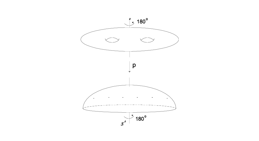
Refer to caption
Figure 9. The Involution ss

Since ss commutes with ii in M2,M_{2}, it descends to a map s~:Σ0,6→Σ0,6.\widetilde{s}:\Sigma_{0,6}\rightarrow\Sigma_{0,6}. We will obtain an expression for s~\widetilde{s} in terms of the generators wiw_{i} and then lift that expression to H2=M2H_{2}=M_{2} via the surjection ψ.\psi.

s~\widetilde{s} is counterclokwise rotation through 180o180{{}^{o}} on Σ0,6,\Sigma_{0,6}, about the axis through the center and the south pole of the sphere, fixing the marked points setwise. It fixes the south pole, therefore forgetting that point we can isotope s~\widetilde{s} to a map s′s^{\prime} of a disc including the 66 marked points, Figure 9. Being an element of M⁡(D,6)=B6,M\left(D,6\right)=B_{6}, s′s^{\prime} can be realized as a braid. Figure 10 (a) and (b) show two different ways of sketching that braid. The first one has the expression

σ1​σ2​σ1​σ3​σ2​σ1​σ4​σ3​σ2​σ1​σ5​σ4​σ3​σ2​σ1\sigma_{1}\sigma_{2}\sigma_{1}\sigma_{3}\sigma_{2}\sigma_{1}\sigma_{4}\sigma_{3}\sigma_{2}\sigma_{1}\sigma_{5}\sigma_{4}\sigma_{3}\sigma_{2}\sigma_{1}

and the second one has the expression

σ5​σ4​σ3​σ2​σ1​σ5​σ4​σ3​σ2​σ5​σ4​σ3​σ5​σ4​σ5.\sigma_{5}\sigma_{4}\sigma_{3}\sigma_{2}\sigma_{1}\sigma_{5}\sigma_{4}\sigma_{3}\sigma_{2}\sigma_{5}\sigma_{4}\sigma_{3}\sigma_{5}\sigma_{4}\sigma_{5}.
Refer to caption
Figure 10. Braids Representing s′s^{\prime} and s′2s^{\prime 2}

Since Figure 10 (a) and (b) are representing isotopic braids, they correspond to the same element in M⁡(D,6).M\left(D,6\right). Therefore

s′2=σ5​σ4​σ3​σ2​σ1​σ5​σ4​σ3​σ2​σ5​σ4​σ3​σ5​σ4​σ5​σ1¯​σ2​σ1¯​σ3​σ2​σ1¯​σ4​σ3​σ2​σ1​σ5​σ4​σ3​σ2​σ1s^{\prime 2}=\sigma_{5}\sigma_{4}\sigma_{3}\sigma_{2}\sigma_{1}\sigma_{5}\sigma_{4}\sigma_{3}\sigma_{2}\sigma_{5}\sigma_{4}\sigma_{3}\sigma_{5}\sigma_{4}\sigma_{5}\underline{\sigma_{1}}\underline{\sigma_{2}\sigma_{1}}\underline{\sigma_{3}\sigma_{2}\sigma_{1}}\sigma_{4}\sigma_{3}\sigma_{2}\sigma_{1}\sigma_{5}\sigma_{4}\sigma_{3}\sigma_{2}\sigma_{1}

which is equal to

σ5​σ4​σ3​σ2​σ1​σ5​σ4​σ3​σ2​σ1¯​σ5​σ4​σ3​σ2​σ1¯​σ5​σ4​σ3​σ2​σ1¯​σ5​σ4​σ3​σ2​σ1​σ5​σ4​σ3​σ2​σ1.\sigma_{5}\sigma_{4}\sigma_{3}\sigma_{2}\sigma_{1}\sigma_{5}\sigma_{4}\sigma_{3}\sigma_{2}\underline{\sigma_{1}}\sigma_{5}\sigma_{4}\sigma_{3}\underline{\sigma_{2}\sigma_{1}}\sigma_{5}\sigma_{4}\underline{\sigma_{3}\sigma_{2}\sigma_{1}}\sigma_{5}\sigma_{4}\sigma_{3}\sigma_{2}\sigma_{1}\sigma_{5}\sigma_{4}\sigma_{3}\sigma_{2}\sigma_{1}.

Thus

s′2=(σ5​σ4​σ3​σ2​σ1)6s^{\prime 2}=\left(\sigma_{5}\sigma_{4}\sigma_{3}\sigma_{2}\sigma_{1}\right)^{6}

using commutativity relations only. It is not difficult to see that this is isotopic to a right handed twist about the boundary of the disk DD, Figure 10 (c). Therefore we have

s~2\displaystyle\widetilde{s}^{2} =\displaystyle= (w5​w4​w3​w2​w1)6\displaystyle\left(w_{5}w_{4}w_{3}w_{2}w_{1}\right)^{6}
=\displaystyle= 1\displaystyle 1

in M⁡(S2,6)M\left(S^{2},6\right) and hence the lift hh of s~\widetilde{s} satisfies

h2=(tc5​tc4​tc3​tc2​tc1)6,h^{2}=\left(t_{c_{5}}t_{c_{4}}t_{c_{3}}t_{c_{2}}t_{c_{1}}\right)^{6},

which is equal to 11 in M2.M_{2}. One needs to check the action of ss and

h=tc1​tc2​tc1​tc3​tc2​tc1​tc4​tc3​tc2​tc1​tc5​tc4​tc3​tc2​tc1h=t_{c_{1}}t_{c_{2}}t_{c_{1}}t_{c_{3}}t_{c_{2}}t_{c_{1}}t_{c_{4}}t_{c_{3}}t_{c_{2}}t_{c_{1}}t_{c_{5}}t_{c_{4}}t_{c_{3}}t_{c_{2}}t_{c_{1}}

on the homology to see that the action of ss is the same as the action of hh, but not as that of h∘ih\circ i [14]. Therefore s=hs=h and

s2=(tc5​tc4​tc3​tc2​tc1)6.s^{2}=\left(t_{c_{5}}t_{c_{4}}t_{c_{3}}t_{c_{2}}t_{c_{1}}\right)^{6}.

Using the braid and commutativity relations it is not difficult to show that

s2=(tc1​tc2​tc3​tc4​tc5)6s^{2}=\left(t_{c_{1}}t_{c_{2}}t_{c_{3}}t_{c_{4}}t_{c_{5}}\right)^{6}

as well.

Another positive Dehn twist expression for s,s, which is of particular interest from topological point of view [16], is

s=tb0​tb1​tb2​tc,s=t_{b_{0}}t_{b_{1}}t_{b_{2}}t_{c},

where b0,b1,b2,b_{0},b_{1},b_{2}, and cc are the cycles shown in Figure 11.

Refer to caption
Figure 11. Another Dehn Twist Expression for ss

Distinguishing the cycle notation from the Dehn twist notation, it is easy to see that

b0\displaystyle b_{0} =\displaystyle= tc1​tc2​tc3​tc4​(c5),\displaystyle t_{c_{1}}t_{c_{2}}t_{c_{3}}t_{c_{4}}\left(c_{5}\right),
b1\displaystyle b_{1} =\displaystyle= tc1​tc1​tc2​tc3​(c4),\displaystyle t_{c_{1}}t_{c_{1}}t_{c_{2}}t_{c_{3}}\left(c_{4}\right),
b2\displaystyle b_{2} =\displaystyle= tc2​tc1​tc1​tc2​(c3).\displaystyle t_{c_{2}}t_{c_{1}}t_{c_{1}}t_{c_{2}}\left(c_{3}\right).

Applying Lemma 1.3.5 we get

tb0\displaystyle t_{b_{0}} =\displaystyle= tc1​tc2​tc3​tc4​tc5​(tc1​tc2​tc3​tc4)−1,\displaystyle t_{c_{1}}t_{c_{2}}t_{c_{3}}t_{c_{4}}t_{c_{5}}\left(t_{c_{1}}t_{c_{2}}t_{c_{3}}t_{c_{4}}\right)^{-1},
tb1\displaystyle t_{b_{1}} =\displaystyle= tc1​tc1​tc2​tc3​tc4​(tc1​tc1​tc2​tc3)−1,\displaystyle t_{c_{1}}t_{c_{1}}t_{c_{2}}t_{c_{3}}t_{c_{4}}\left(t_{c_{1}}t_{c_{1}}t_{c_{2}}t_{c_{3}}\right)^{-1},
tb2\displaystyle t_{b_{2}} =\displaystyle= tc2​tc1​tc1​tc2​tc3​(tc2​tc1​tc1​tc2)−1.\displaystyle t_{c_{2}}t_{c_{1}}t_{c_{1}}t_{c_{2}}t_{c_{3}}\left(t_{c_{2}}t_{c_{1}}t_{c_{1}}t_{c_{2}}\right)^{-1}.

Therefore the product tb0​tb1​tb2t_{b_{0}}t_{b_{1}}t_{b_{2}} becomes

tc1​tc2​tc3​tc4​tc5​(tc1​tc2​tc3​tc4)−1​tc1​tc1​tc2​tc3​tc4​(tc1​tc1​tc2​tc3)−1​tc2​tc1​tc1​tc2​tc3​(tc2​tc1​tc1​tc2)−1.t_{c_{1}}t_{c_{2}}t_{c_{3}}t_{c_{4}}t_{c_{5}}\left(t_{c_{1}}t_{c_{2}}t_{c_{3}}t_{c_{4}}\right)^{-1}t_{c_{1}}t_{c_{1}}t_{c_{2}}t_{c_{3}}t_{c_{4}}\left(t_{c_{1}}t_{c_{1}}t_{c_{2}}t_{c_{3}}\right)^{-1}t_{c_{2}}t_{c_{1}}t_{c_{1}}t_{c_{2}}t_{c_{3}}\left(t_{c_{2}}t_{c_{1}}t_{c_{1}}t_{c_{2}}\right)^{-1}.

We also have tc=(tc1​tc2​tc1)4=(tc1​tc2)6=(tc2​tc1)6t_{c}=\left(t_{c_{1}}t_{c_{2}}t_{c_{1}}\right)^{4}=\left(t_{c_{1}}t_{c_{2}}\right)^{6}=\left(t_{c_{2}}t_{c_{1}}\right)^{6} using the braid relation and the special case of the chain relation on the subsurface Σ11\Sigma_{1}^{1}.

Next, we will simplify the expression for the product tb0​tb1​tb2.t_{b_{0}}t_{b_{1}}t_{b_{2}}. We will use just the indices representing the twists for brevity. For example 11 will mean tc1t_{c_{1}}, 22 will mean tc2t_{c_{2}}, etc. The change in each line occurs within the underlined portion of the entire expression and the result of that change is not underlined in the next line. We only use commutativity and braid relations.

tb0​tb1​tb2\displaystyle t_{b_{0}}t_{b_{1}}t_{b_{2}} =\displaystyle= 12345​(1¯​234)−1​1¯​1234​(1123)−1​21123​(2112)−1\displaystyle 12345\left(\underline{1}234\right)^{-1}\underline{1}1234\left(1123\right)^{-1}21123\left(2112\right)^{-1}
=\displaystyle= 12345​(234)−1​1234¯​(1123)−1​21123​(2112)−1\displaystyle 12345\underline{\left(234\right)^{-1}1234}\left(1123\right)^{-1}21123\left(2112\right)^{-1}
=\displaystyle= 123451234​(123)−1​(11¯​23)−1​21123​(2112)−1\displaystyle 123451234\left(123\right)^{-1}\left(\underline{11}23\right)^{-1}21123\left(2112\right)^{-1}
=\displaystyle= 123451234​(123)−1​(23)−1​(11)−1¯​21123​(2112)−1\displaystyle 123451234\left(123\right)^{-1}\left(23\right)^{-1}\underline{\left(11\right)^{-1}}21123\left(2112\right)^{-1}
=\displaystyle= 123451234​(123)−1​(2¯​3)−1​21123​(11)−1​(2112)−1\displaystyle 123451234\left(123\right)^{-1}\left(\underline{2}3\right)^{-1}21123\left(11\right)^{-1}\left(2112\right)^{-1}
=\displaystyle= 123451234​(123)−1​(3)−1¯​1123​(11)−1​(2112)−1\displaystyle 123451234\left(123\right)^{-1}\underline{\left(3\right)^{-1}}1123\left(11\right)^{-1}\left(2112\right)^{-1}
=\displaystyle= 123451234​(1¯​23)−1​1123​(2)−1​(11)−1​(2112)−1\displaystyle 123451234\left(\underline{1}23\right)^{-1}1123\left(2\right)^{-1}\left(11\right)^{-1}\left(2112\right)^{-1}
=\displaystyle= 123451234​(23)−1¯​123​(2)−1​(11)−1​(2112)−1\displaystyle 123451234\underline{\left(23\right)^{-1}}123\left(2\right)^{-1}\left(11\right)^{-1}\left(2112\right)^{-1}
=\displaystyle= 123451234123​(12)−1​(2)−1​(11)−1​(2112)−1\displaystyle 123451234123\left(12\right)^{-1}\left(2\right)^{-1}\left(11\right)^{-1}\left(2112\right)^{-1}
=\displaystyle= 123451234123​1211−1​(12)−1¯​(12)−1​(2)−1​(11)−1​(2112)−1\displaystyle 123451234123\underline{1211^{-1}\left(12\right)^{-1}}\left(12\right)^{-1}\left(2\right)^{-1}\left(11\right)^{-1}\left(2112\right)^{-1}
=\displaystyle= 1234512341231211−1​2−1​1−1​2−1​1−1​2−1​1−1​1−1​2−1​1−1¯​1−1​2−1\displaystyle 1234512341231211^{-1}2^{-1}1^{-1}2^{-1}1^{-1}2^{-1}1^{-1}\underline{1^{-1}2^{-1}1^{-1}}1^{-1}2^{-1}
=\displaystyle= 1234512341231211−1​2−1​1−1​2−1​1−1​2−1​1−1​2−1​1−1​2−1​1−1​2−1\displaystyle 1234512341231211^{-1}2^{-1}1^{-1}2^{-1}1^{-1}2^{-1}1^{-1}2^{-1}1^{-1}2^{-1}1^{-1}2^{-1}
=\displaystyle= 123451234123121​(1−1​2−1)6\displaystyle 123451234123121\left(1^{-1}2^{-1}\right)^{6}
=\displaystyle= 123451234123121​(21)−6.\displaystyle 123451234123121\left(21\right)^{-6}.

Now using the fact that tc=(21)6t_{c}=\left(21\right)^{6} we get

tb0​tb1​tb2​tc\displaystyle t_{b_{0}}t_{b_{1}}t_{b_{2}}t_{c} =\displaystyle= 123451234123121​(21)−6​(21)6,\displaystyle 123451234123121\left(21\right)^{-6}\left(21\right)^{6},
tb0​tb1​tb2​tc\displaystyle t_{b_{0}}t_{b_{1}}t_{b_{2}}t_{c} =\displaystyle= 123451234123121,\displaystyle 123451234123121,

i.e.,

s=tb0​tb1​tb2​tc=tc1​tc2​tc3​tc4​tc5​tc1​tc2​tc3​tc4​tc1​tc2​tc3​tc1​tc2​tc1.s=t_{b_{0}}t_{b_{1}}t_{b_{2}}t_{c}=t_{c_{1}}t_{c_{2}}t_{c_{3}}t_{c_{4}}t_{c_{5}}t_{c_{1}}t_{c_{2}}t_{c_{3}}t_{c_{4}}t_{c_{1}}t_{c_{2}}t_{c_{3}}t_{c_{1}}t_{c_{2}}t_{c_{1}}.

To see that this is the same expression that we obtained earlier:

s\displaystyle s =\displaystyle= tc1​tc2​tc3​tc4​tc5​tc1¯​tc2​tc3​tc4​tc1​tc2​tc3​tc1​tc2​tc1\displaystyle t_{c_{1}}t_{c_{2}}t_{c_{3}}t_{c_{4}}t_{c_{5}}\underline{t_{c_{1}}}t_{c_{2}}t_{c_{3}}t_{c_{4}}t_{c_{1}}t_{c_{2}}t_{c_{3}}t_{c_{1}}t_{c_{2}}t_{c_{1}}
=\displaystyle= tc1​tc2​tc1​tc3​tc4​tc5​tc2¯​tc3​tc4​tc1¯​tc2​tc3​tc1​tc2​tc1\displaystyle t_{c_{1}}t_{c_{2}}t_{c_{1}}t_{c_{3}}t_{c_{4}}t_{c_{5}}\underline{t_{c_{2}}}t_{c_{3}}t_{c_{4}}\underline{t_{c_{1}}}t_{c_{2}}t_{c_{3}}t_{c_{1}}t_{c_{2}}t_{c_{1}}
=\displaystyle= tc1​tc2​tc1​tc3​tc2​tc1​tc4​tc5​tc3¯​tc4​tc2¯​tc3​tc1¯​tc2​tc1\displaystyle t_{c_{1}}t_{c_{2}}t_{c_{1}}t_{c_{3}}t_{c_{2}}t_{c_{1}}t_{c_{4}}t_{c_{5}}\underline{t_{c_{3}}}t_{c_{4}}\underline{t_{c_{2}}}t_{c_{3}}\underline{t_{c_{1}}}t_{c_{2}}t_{c_{1}}
=\displaystyle= tc1​tc2​tc1​tc3​tc2​tc1​tc4​tc3​tc2​tc1​tc5​tc4​tc3​tc2​tc1.\displaystyle t_{c_{1}}t_{c_{2}}t_{c_{1}}t_{c_{3}}t_{c_{2}}t_{c_{1}}t_{c_{4}}t_{c_{3}}t_{c_{2}}t_{c_{1}}t_{c_{5}}t_{c_{4}}t_{c_{3}}t_{c_{2}}t_{c_{1}}.

For an excellent treatment of this work for general case see [9].

2. Main Theorem

The hyperelliptic involution i:f:Σh→Σhi:f:\Sigma_{h}\rightarrow\Sigma_{h} and the involution s:Σk→Σks:\Sigma_{k}\rightarrow\Sigma_{k} that were described in section 1.4 can be combined into an involution θ:\theta: Σh+k→Σh+k\Sigma_{h+k}\rightarrow\Sigma_{h+k} that supports the action of both ii ands\ s on bounded subsurfaces of Σh+k\Sigma_{h+k} as shown in Figure 12.

Refer to caption
Figure 12. The Involution θ\theta
Refer to caption
Figure 13. Base Cycles

The main theorem gives a positive Dehn twist expression for θ.\theta. We will use the same notation for both the cycles and the Dehn twists about them throughout the section. The order of the product is from right to left.

Theorem 2.0.1.

The positive Dehn twist expression for the involution that is shown in Figure 12 is given by

θ=c2​i+2⋯c2​hc2​h+1c2​i⋯c2c1b0c2​h+1c2​h⋯c2​i+2c1c2⋯c2​ib1b2⋯bk−1bkc2​i+1.\theta=c_{2i+2}\cdots c_{2h}c_{2h+1}c_{2i}\cdots c_{2}c_{1}b_{0}c_{2h+1}c_{2h}\cdots c_{2i+2}c_{1}c_{2}\cdots c_{2i}b_{1}b_{2}\cdots b_{k-1}b_{k}c_{2i+1}.

Proof: Figure 13 shows a set of cycles that will constitute a base in the sense that, mapping of those cycles will ensure the mapping of the subsurfaces that they bound accordingly. Therefore, it suffices to check the images of those cycles under θ\theta and see that they are mapped to the correct places. Furthermore, for cycle pairs that are symmetrical with respect to the vertical axis through the center of the figure, we will look at the mapping of those that are on the right hand side only. The mapping of their counterpart goes similarly due to symmetry. Finally, Figure 22 shows an example for the mapping of separating cycles.

First we will see the mapping of cjc_{j} for j≠2​i,2​i+1j\neq 2i,2i+1 or 2​i+2.2i+2. Figure 14 shows the mapping of such a cycle for 2​i+3≤j≤2​h+12i+3\leq j\leq 2h+1. Whether cjc_{j} goes around a hole or goes through two holes, only two twists are effective in its mapping: cjc_{j} and cj−1c_{j-1}.

Refer to caption
Figure 14. Mapping of cjc_{j}

Next, we will find the image of djd_{j} for 2≤j≤h−1.2\leq j\leq h-1. Figure 15 shows the mapping of djd_{j} for i+1≤j≤h−1.i+1\leq j\leq h-1. As the figure indicates the twists along bj,j=0,1,…,kb_{j},j=0,1,\ldots,k do not take part in mapping of djd_{j}. This is true for did_{i} and di+1d_{i+1} as well.

Refer to caption
Figure 15. Mapping of djd_{j}

Figure 16 shows how c2​i+2c_{2i+2} is mapped. The mapping of c2​ic_{2i} is similar, therefore we omit the proof.

[Uncaptioned image]
Refer to caption
Figure 16. Mapping of c2​i+2c_{2i+2}

Figure 17 shows the mapping of e1.b0e_{1}.\,b_{0} is effective in the mapping of e1e_{1} as the figure indicates and it does not take part in the mapping of ei,i=2,…,2​k.e_{i},i=2,\ldots,2k. The mapping of e2​k+1e_{2k+1} is the same as that of e1e_{1}, therefore its proof is omitted. The cycle to which b0b_{0} is applied looks different in the third line but they are isotopic.

Refer to caption
Figure 17. Mapping of e1e_{1}

The mapping of e2e_{2} is shown in the first two lines of Figure 18. The mapping of eje_{j} for j−j- even is similar to that of e2e_{2}, including eke_{k}. The mapping of e2​j−1,j=2,…,k/2e_{2j-1},j=2,\ldots,k/2 is shown in the last two lines of the same figure. The proof for the mapping of ej,j=k+2,…,2​ke_{j},j=k+2,\ldots,2k is similar, therefore omitted.

Refer to caption
Figure 18. Mappings of e2e_{2} and e2​j−1,j=2,…,k/2e_{2j-1},j=2,\ldots,k/2

Figure 19 shows the mapping of fk/2f_{k/2} and the mapping of fj,j=2,…,k/2−1f_{j},j=2,\ldots,k/2-1 are the same. We omit the proof for fj,j=k/2+1,…,kf_{j},j=k/2+1,\ldots,k due to the same reason. The cycle to which the twist about b0b_{0} is applied in the last line looks different in the previous figure but they are isotopic.

Refer to caption
Figure 19. Mapping of fk/2f_{k/2}

The mapping of a2a_{2} is shown in Figure 20. The proof for the mapping of its mirror image is omitted because of the symmetry.

Refer to caption
Figure 20. Mapping of a2a_{2}

Figure 21 shows the mapping of c2​i+1c_{2i+1}. Since c2​i+1∩bk=2c_{2i+1}\cap b_{k}=2, we have tbk​(c2​i+1)=bk2​c2​i+1t_{b_{k}}(c_{2i+1})=b_{k}^{2}\ c_{2i+1} by Lemma 1.3.3. Also since tbk​(c2​i+1)∩bk−1=2t_{b_{k}}(c_{2i+1})\ \cap\ b_{k-1}=2 we have tbk−1​(tbk​(c2​i+1))=bk−12​(bk2​c2​i+1).t_{b_{k-1}}(t_{b_{k}}(c_{2i+1}))=b_{k-1}^{2}\ (b_{k}^{2}\ c_{2i+1}). Lemma 1.3.3 applies to all bj,j=0,…,kb_{j},j=0,\ldots,k because each of them intersects the curve they are applied to twice.

[Uncaptioned image]
Refer to caption
Figure 21. Mapping of c2​i+1c_{2i+1}

Figure 22 shows the mapping of a separating cycle.

[Uncaptioned image]
[Uncaptioned image]
Refer to caption
Figure 22. Mapping of a Separating Cycle

3. Applications

Next, we will compute the homeomorphism invariants of the genus gg Lefschetz fibrations

X⟶S2X\longrightarrow S^{2}

described by the involution θ\theta that was defined in Theorem 2.0.1, namely by the word θ2=1\theta^{2}=1 in MgM_{g}, for some small values of gg. Consider the surface in Figure 12. Let kk denote the genus of the central part of the figure, which we will call the vertical genus. Let l be the total genus on the left and r be the total genus on the right of the vertical component. Let h be the horizontal genus, namely the sum of the left genus and the right genus; so, h=l+r.h=l+r. If we denote the total genus by gg then g=h+k=l+r+kg=h+k=l+r+k. A quick check reveals that the total number of twists in the word θ2=1\theta^{2}=1 is 8​h+2​k+4=2​g+4+6​h8h+2k+4=2g+4+6h.

Using the algorithm described in [17] we wrote a Matlab program that computes the signature of the manifold described by the word θ2=1\theta^{2}=1 for given l,r,l,r, and kk. The following table lists the output of the program for a few values of l,r,l,r, and kk. The first column is for the input of the program in the format (l,k,r)(l,k,r), the second column is for the horizontal genus h=l+rh=l+r, the third column is for the vertical genus kk, the fourth column is for the total genus g=h+kg=h+k, the fifth column is for the word length w=8​h+2​k+4,w=8h+2k+4, and the last column is for the output of the program, which is the signature of the manifold for the given triple (l,k,r)(l,k,r).

(l,k,r) h=l+r k g=h+k w=8h+2k+4 signature
(1,2,1) 2 2 4 24 -12
(1,4,1) 2 4 6 28 -12
(1,6,1) 2 6 8 32 -12
(1,8,1) 2 8 10 36 -12
(1,10,1) 2 10 12 40 -12
(2,2,1) 3 2 5 32 -16
(1,2,2) 3 2 5 32 -16
(2,4,1) 3 4 7 36 -16
(1,4,2) 3 4 7 36 -16
(2,6,1) 3 6 9 40 -16
(1,6,2) 3 6 9 40 -16
(2,8,1) 3 8 11 44 -16
(1,8,2) 3 8 11 44 -16
(3,2,1) 4 2 6 40 -20
(2,2,2) 4 2 6 40 -20
(1,2,3) 4 2 6 40 -20
(3,4,1) 4 4 8 44 -20
(2,4,2) 4 4 8 44 -20
(1,4,3) 4 4 8 44 -20
(3,6,1) 4 6 10 48 -20
(2,6,2) 4 6 10 48 -20
(1,6,3) 4 6 10 48 -20
(3,8,1) 4 8 12 52 -20
(2,8,2) 4 8 12 52 -20
(1,8,3) 4 8 12 52 -20

The outputs consist of 00’s and −1-1’s only. The order in which they appear is the same for a fixed value of hh and kk in all the examples above. In other words the order in which the signature contributions of the 2−2- handles appear does not depend on how the horizontal genus is distributed to left and right, once we fix hh and kk. Therefore we will not record ll and rr for the rest of the examples.

h k g=h+k w=8h+2k+4 signature
5 2 7 48 -24
5 4 9 52 -24
5 6 11 56 -24
5 8 13 60 -24
6 2 8 56 -28
6 4 10 60 -28
6 6 12 64 -28
6 8 14 68 -28
7 2 9 64 -32
7 4 11 68 -32
7 6 13 72 -32
8 2 10 72 -36
8 4 12 76 -36
8 6 14 80 -36

The signature values in the tables above are statistically convincing that the signature of the Lefschetz fibration given by the word θ2=1\theta^{2}=1 must be

σ​(X)=−4​(h+1).\sigma(X)=-4(h+1).

We do not know a topological proof for that; however, for a proof of this claim for h=0,1h=0,1 the reader is referred to [9].

All of the Dehn twists appearing in the expression for θ\theta are about nonseparating cycles. Therefore the Lefschetz fibration that is given by the word θ2=1\theta^{2}=1 has

8​h+2​k+48h+2k+4

irreducible singular fibers and its Euler characteristic χ⁡(X)\chi(X) is

χ⁡(X)\displaystyle\chi\left(X\right) =\displaystyle= 2​(2−2​g)+8​h+2​k+4\displaystyle 2\left(2-2g\right)+8h+2k+4
=\displaystyle= 2​(2−2​(h+k))+8​h+2​k+4\displaystyle 2\left(2-2(h+k)\right)+8h+2k+4
=\displaystyle= 8+4​h−2​k.\displaystyle 8+4h-2k.

For the values of the Euler characteristic and the signature above, c12​(X)c_{1}^{2}(X) and χh​(X)\chi_{h}(X) are

c12​(X)\displaystyle c_{1}^{2}(X) =\displaystyle= 3​σ​(X)+2​χ​(X)\displaystyle 3\sigma(X)+2\chi(X)
=\displaystyle= 3​(−4​h−4)+2​(8+4​h−2​k)\displaystyle 3(-4h-4)+2(8+4h-2k)
=\displaystyle= −4​h−4​k+4\displaystyle-4h-4k+4
=\displaystyle= −4​(g−1)\displaystyle-4(g-1)

and

χh​(X)\displaystyle\chi_{h}(X) =\displaystyle= 14​(σ​(X)+χ​(X))\displaystyle\frac{1}{4}(\sigma(X)+\chi(X))
=\displaystyle= 14​(8+4​h−2​k−4​h−4)\displaystyle\frac{1}{4}(8+4h-2k-4h-4)
=\displaystyle= 14​(4−2​k)=1−k/2\displaystyle\frac{1}{4}(4-2k)=1-k/2

χh​(X)\chi_{h}(X) in the above computation makes sense because XX has almost complex structure. It is an integer since kk is even.

The following are the actual computer outputs for the signature computations for the indicated values of (l,k,r)(l,k,r).

(l,k,r)(l,k,r) output
(1,2,1) 0 +0 +0 +0 +0 +0 -1 -1 -1 -1 -1 -1
-1 -1 +0 -1 -1 -1 -1 +0 +0 +0 +0 +0 = -12
(1,4,1) 0 +0 +0 +0 +0 +0 +0 +0 -1 -1 -1 -1 -1 -1
-1 -1 +0 +0 +0 -1 -1 -1 -1 +0 +0 +0 +0 +0 = -12
(1,6,1) 0 +0 +0 +0 +0 +0 +0 +0 +0 +0 -1 -1 -1 -1 -1 -1
-1 -1 +0 +0 +0 +0 +0 -1 -1 -1 -1 +0 +0 +0 +0 +0 = -12
(2,2,1) 0 +0 +0 +0 +0 +0 +0 +0 -1 -1 -1 -1 -1 -1 -1 -1
-1 -1 +0 -1 -1 -1 -1 -1 -1 +0 +0 +0 +0 +0 +0 +0= -16
(2,2,2) 0 +0 +0 +0 +0 +0 +0 +0 +0 +0 -1 -1 -1 -1 -1 -1 -1 -1 -1 -1
-1 -1 +0 -1 -1 -1 -1 -1 -1 -1 -1 +0 +0 +0 +0 +0 +0 +0 +0 +0
= -20
(2,4,2) 0 +0 +0 +0 +0 +0 +0 +0 +0 +0 +0 +0 -1 -1 -1 -1 -1 -1 -1 -1
-1 -1 -1 -1 +0 +0 +0 -1 -1 -1 -1 -1 -1 -1 -1 +0 +0 +0 +0 +0
+0 +0 +0 +0 = -20
(l,k,r)(l,k,r) output
(3,2,2) 0 +0 +0 +0 +0 +0 +0 +0 +0 +0 +0 +0 -1 -1 -1 -1
-1 -1 -1 -1 -1 -1 -1 -1 -1 -1 +0 -1 -1 -1 -1 -1
-1 -1 -1 -1 -1 +0 +0 +0 +0 +0 +0 +0 +0 +0 +0 +0= -24
(4,2,4) 0 +0 +0 +0 +0 +0 +0 +0 +0 +0 +0 +0 +0 +0 +0 +0 +0 +0
-1 -1 -1 -1 -1 -1 -1 -1 -1 -1 -1 -1 -1 -1 -1 -1 -1 -1
-1 -1 +0 -1 -1 -1 -1 -1 -1 -1 -1 -1 -1 -1 -1 -1 -1 -1
-1 +0 +0 +0 +0 +0 +0 +0 +0 +0 +0 +0+0 +0 +0 +0 +0 +0
= -36

Acknowledgment I would like to express my deepest gratitude to my thesis advisor Ronald J. Stern for his continuous support and guidance.

References

  • [1] J. Birman, Braids, links, and mapping class groups, Ann. of Math. Studies, 82, Princeton Uni. Press, Princeton, 1975.
  • [2] M. Dehn, Die Gruppe der Abbildungsklassen, Acta Math. 69 (1938), 135-206.
  • [3] S. Donaldson, Lefschetz fibrations in symplectic geometry, Doc. Math. J. DMV., Extra Volume, ICMII (1998), 309-314.
  • [4] A. Fathi, F. Laudenbach, and V. Poénaru, Travaux de Thurston sur les surfaces, Séminaire Orsay, Astérisque, (1979), 66-67.
  • [5] R.Gompf and A.Stipsicz, An Introduction to 4-manifolds and Kirby Calculus, AMS Graduate Studies in Mathematics, 20 (1999).
  • [6] S. Humphries, Generators for the mapping class group, Topology of low-dimensional manifolds, LNM 722 (1979), 44-47.
  • [7] N.V. Ivanov, Mapping class groups, Handbook of geometric topology, to appear.
  • [8] D. Johnson, Homeomorphisms of a surface which act trivially on homology, Proc. Amer. Math. Soc., 75 (1979), 119-125.
  • [9] M. Korkmaz, Noncomplex smooth 4-manifolds with Lefschetz fibrations, International Mathematics Research Notices, 3 2001.
  • [10] W.B.R. Lickorish, A finite set of generators for the homology group of a 2−2- manifold, Proc. Camb. Philos. Soc., 60 (1964), 769-778.
  • [11] F. Luo, A presentation of the mapping class groups in surfaces, preprint, arXiv:math.GT/9801025.
  • [12] F. Luo, Some applications of a multiplicative structure on simple loops in surfaces, preprint, arXiv:math.GT/9907059.
  • [13] L. Paris, D. Rolfsen, Geometric subgroups of mapping class groups, preprint, arXiv:math.GT/9906122.
  • [14] J.D. McCarthy and A.Papadopoulos, Involutions in surface mapping class groups, Enseign. Math., 2 33 (1987), 275-290.
  • [15] D. Margalit, A lantern lemma, Algebraic and Geometric Topology , 2 (2002) 1179-1195.
  • [16] Y.Matsumoto, Lefschetz fibrations of genus 22 - A topological approach, Topology and Teichmüller Spaces (Katinkulta, Finland, 1995), World Sci., River Edge, NJ, (1996), 123-148.
  • [17] B.Ozbagci, Signatures of Lefschetz fibrations, Pacific Journal of Mathematics, Vol. 202 1 (2002), 99-118.
  • [18] B.Wajnryb, A simple presentation for the mapping class group of an orientable surface, Israel J. Math., 45 (1983), 157-174.
  • [19] B.Wajnryb, Mapping class group of a surface is generated by two elements, Topology, 35 (1996), 377-383.
  • [20] B.Wajnryb, An elementary approach to the mapping class group of a surface, Geometry & Topology, 3 (1999), 405-466.