A tropical morphism related to the hyperplane arrangement of the complete bipartite graph
Abstract
We undertake a combinatorial study of the piecewise linear map which assigns to the four vectors in and in the matrix given by . This map arises naturally in Pachter and Sturmfels’s work on the tropical geometry of statistical models. The image of has been a subject of recent interest; it is the positive part of the tropical algebraic variety which parameterizes -tuples of points on a tropical line in -space.
The domains of linearity of are the regions of the real hyperplane arrangement , corresponding to the complete bipartite graph . We explain how the images of (some of) the regions provide two polyhedral subdivisions of the image of , one of which is a refinement of the other. The finer subdivision is particularly nice enumeratively: it has maximum-dimensional cells, where is the number of regions of the arrangement .
1 Introduction
0. The goal of this paper is to undertake a combinatorial study of the piecewise linear map given by
where and denote vectors in and and denote vectors in .
The paper is organized as follows. In Section 2, we describe and enumerate the domains of linearity of the map ; they are precisely the faces of the arrangement , corresponding to the complete bipartite graph . In Section 3 we describe the images , as ranges over the regions of the arrangement. In Section 4 we show that these images fit together in an unusual way to give the full image ; as a consequence, we obtain two different polyhedral subdivisions of , one of which is a refinement of the other. The finer subdivision is particularly nice combinatorially; the number of its facets is , where is the number of regions of the arrangement .
This project was suggested in a recent paper of Pachter and Sturmfels [17]. It arose in their study of the tropical geometry of statistical models, and provides a new perspective on Develin, Santos and Sturmfels’s study of the image of [9, 10].
To explain their motivation, we start with a brief overview of some recent developments in tropical geometry which led to its consideration.
1. The tropical semiring is the set of real numbers augmented by infinity, together with the operations of tropical addition and multiplication, which are defined by and
Tropical algebraic geometry is, roughly speaking, the geometry of the tropical semiring. Let be the (algebraically closed) ring of Puiseux series; its elements are formal power series of the form , where are rational numbers with a common denominator. There is a natural valuation , which sends the non-zero Puiseux series to its degree .
For an ideal in , let be the corresponding algebraic variety, intersected with the torus . It consists of the -tuples of non-zero Puiseux series such that for all . Define .
Theorem.
Let be the set of -tuples in such that the coefficient of the leading term of each is a positive real number.
Theorem.
[20] For an ideal in , the following subsets of coincide.
- 1.
The topological closure of .
- 2.
The set of such that .
This set is called the positive part of the tropical variety of , and denoted .
For all , is a polyhedral complex, and is a subcomplex of it.
2. Let be a polynomial map. Say that is positive if each polynomial has only positive coefficients. Say that is surjectively positive if, additionally, every point in the image of whose coordinates are positive has a preimage whose coordinates are positive; i.e., .
The tropicalization of is the piecewise linear map obtained from by replacing every with a and every with a . Such a map is called a tropical morphism. [17]
The relationship between the positive part of a tropical variety and morphisms is outlined in the following theorem.
Theorem.
3. Pachter and Sturmfels [17] used this setup to study the tropical geometry of statistical models. The naive Bayes model with two features [13] is parameterized by the polynomial map which maps an matrix and a matrix to their product. Its tropicalization, , is the object of study of this paper.
The image of consists of the real matrices of rank at most . This is an algebraic variety, whose corresponding prime ideal is generated by the subdeterminants of an matrix.
The tropical variety is the set of real matrices having tropical rank at most , and the positive part is the set of real matrices having Barvinok rank at most . For the relevant definitions and further information, see [9, 10, 17].
This model interests us because the map is surjectively positive:
Theorem.
[8] Every positive matrix of rank can be written as the product of a positive matrix and a positive matrix.
It follows that .
The study of the map is therefore closely related to Pachter and Sturmfels’s study of the tropical geometry of statistical models, and to Develin, Santos and Sturmfels’s study of the space .
2 The morphism and its domains of linearity.
The piecewise linear map which we wish to study is the tropicalization of matrix multiplication; it is given by
Here and denote vectors in and and denote vectors in . Let and . The entry of is given by
The piecewise linear map is linear on the faces of the hyperplane arrangement in :
This is essentially the graphical arrangement of the complete bipartite graph ; it contains one hyperplane for each edge of .
Therefore, to understand the fibers of the map , we first study the faces of .
Let us briefly outline the close connection between the arrangement and the graph . The matroid associated to the arrangement is isomorphic to the matroid associated to the graph. In other words, a subset of hyperplanes of intersects in codimension if and only if the corresponding subset of edges of does not contain a cycle. Let us call this matroid simply ; it encodes much of the combinatorial information of the arrangement of the graph. For more details, see [15, Ch. 2] or [16, Ch.5].
The regions of the arrangement are in one-to-one correspondence with the acyclic orientations of the bipartite graph , as follows: Denote the vertices of by , and consider an acyclic orientation of . The corresponding region consists of the points such that if the edge is directed in , and otherwise.
The matroid appeared independently in the work of Martin and Reiner [14]. They used the finite field method of [1] to compute a generating function for , the coboundary polynomial of . This polynomial is a simple transformation of the Tutte polynomial, and it captures much of the interesting enumerative information of the matroid.
Proposition.
[14] If is the coboundary polynomial of ,
Corollary.
[21, Ex. 5.6] Let be the number of acyclic orientations of (or equivalently, the number of regions of ). Then
Proof.
This follows from the formula [23] for the number of regions of a real arrangement. ∎
We now proceed to describe and count the domains of linearity of ; that is, the faces of the arrangement .
Proposition 1.
Let be the number of -dimensional faces of the arrangement . Then
Proof.
To describe a face of the arrangement we must specify, for each hyperplane , whether is in the halfspace , in the halfspace , or on the hyperplane . Consider the inequalities or equalities that define a face . Each one of them puts a restriction on the relative order of the variables . For a point in , the relative order of and is determined for all and . The relative order of and is not always determined: an equality can only be deduced from two defining equalities of the form and . Similarly, an inequality can only be deduced as a consequence of two defining inequalities or equalities of the form and .
The faces of are described putting these restrictions together. For example, one face of consists of the points such that
Each face of can be described in a similar way, as a sequence of blocks of variables. The variables and are in the same block if the comparisons and yield the same result for each . A similar statement holds for and . The variables and are in the same block if in .
Call a block positive if it only contains s, negative if it only contains s, and mixed otherwise. For a point to belong to the face, the variables within each mixed block are equal. Within an unmixed block, the relative order of the variables is not determined.
It follows that the faces of are in one-to-one correspondence with the ordered partitions of the set containing no two consecutive unmixed blocks of the same sign. The dimension of a face is easily determined from the partition: it is equal to the sum of the sizes of the unmixed blocks plus the number of mixed blocks. We can now use the methods of [21, Chapter 5] to compute the desired generating function.
The generating function for non-empty positive blocks is . The generating function for non-empty negative blocks is . Therefore, the generating function for partitions of into unmixed blocks of alternating sign is
On the other hand, the generating function for mixed blocks is given by . The partitions we wish to count are alternating sequences of partitions of the type counted by (which may be empty) and mixed blocks. Therefore
which is equal to the given expression.
∎
Observe that, under the above correspondence, the regions of correspond to the ordered partitions which contain no mixed blocks. These are counted by ; setting recovers the generating function for .
It will be convenient to label each region of the arrangement with the permutation of the set obtained by reading the blocks from left to right. The variable corresponds to the letter (which we call a positive letter), and the variable corresponds to the letter (which we call a negative letter). Within each block, the letters are arranged in increasing order.
For example, the region
of is simply denoted by the permutation .
This labelling is a bijection between the regions of and the permutations of such that any two consecutive letters of the same sign are in increasing order.
3 The image of in each region
Consider a region of . As we mentioned earlier, the restriction of the map to the region is a linear function. We now describe the image .
Color each entry of the matrix either black or white: the entry is black if in , and white if in . Permute the rows and columns of according to the order in which their labels appear in . A path separates the white and black entries: it starts at the northwest corner of the matrix, and takes a step south for each positive letter in and a step east for each negative letter in , in the order prescribed by .

Figure 1 shows the resulting matrix and path for . The entry is if it is below or if it is above . We call this picture the diagram of or of .
For , write
For simplicity, we will omit from the notation and simply write for this expression. We will call an equality or inequality of the form a rectangle relation. Write when appears before in .
Proposition 2.
(Version 1.) The image is an open polytope, described by the rectangle equalities and inequalities that it satisfies. They are the following:
and no others.
In the diagram of , let be the sub-rectangle of the diagram containing rows through and columns through . (We implicitly assume that and in .) Call this sub-rectangle monochromatic if all its entries have the same color. Call it sliced if it has black and white entries, separated by a single vertical or horizontal line. Call it jagged otherwise. These definitions are illustrated in Figure 2.
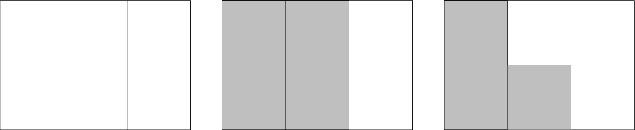
Proposition 2.
(Version 2.) The image consists of those such that is:
- •
equal to zero if is monochromatic,
- •
positive if is jagged.
(If is sliced, takes positive and negative values in .)
Proof.
It is straightforward to verify that the two versions of Proposition 2 are equivalent. Consider a point in . The entry of is given by if it is white (i.e. if in ), or if it is black (i.e. if in ). These entries are easily seen to satisfy the given equalities and inequalities.
Conversely, consider a matrix which satisfies the given equalities and inequalities. Permute its columns and rows according to the order in which their labels appear in , and draw the path .
Choose appropriate values of the s and s so that for all the southernmost and westernmost black entries (the ones surrounded by a box in Figure 1). This can be done because the system of equations is independent, and has more unknowns than equations. Make the s and s which do not appear in this system of equations very large positive numbers. Similarly, choose appropriate values of the s and s so that for all the northernmost and easternmost white entries, and make the other s and s very large positive numbers.
Since satisfies the rectangle equalities of , for all black entries and for all the white entries.
Take a black entry . If the northernmost entry on its column or the easternmost entry on its row is black, then is a very large positive number, larger than . Otherwise, the rectangle determined by it and the northeasternmost corner of the matrix has three white entries and one black entry, and the corresponding rectangle inequality is equivalent to . Similarly, for white entries . Therefore and .
∎
Corollary.
Let be a region of . Then is the subspace of described by the equalities
for those such that and have the same color.
For a region let be the length of the first block of letters of of the same sign (or equivalently, the number of sources of the corresponding orientation ), and let be the length of the last block of letters of of the same sign (or equivalently, the number of sinks of ).
Let be the region where for all and , and let be the region where for all and .
Corollary.
Let be a region of . If , then
Otherwise, .
Proof.
The southernmost and westernmost black entries and the northernmost and easternmost white entries linearly generate the remaining ones, and there are no linear relations among them. The number of them is as claimed. ∎
In particular, the regions where has maximum rank are those corresponding to acyclic orientations of with a unique source and a unique sink. This maximum rank is equal to .
4 Two subdivisions of the image of .
The closures of the regions of the hyperplane arrangement give a polyhedral covering of . Their images under the map give a covering of the full image, . We now wish to understand how the images of the closures of the regions , which we call the cells, fit together.
First notice that if is a region of and is its negative (so the permutation is equal to the permutation reversed), then it follows from Proposition 2 that . Therefore, we can restrict our attention only to the positive regions, where (or equivalently, in ).
Also, the following proposition shows that it suffices to study the maximum-dimensional cells.
Proposition.
[9] The image is pure.
Interestingly, though, our collection of cells is not pure-dimensional. For example, the image of the region is a subspace which is not contained in any maximum-dimensional cell.
Recall that the cell is maximum-dimensional if and only if the first and the last block of are singletons. Call such a maximum-dimensional cell large if the second and the second-to-last blocks of are not singletons, small if the second and the second-to-last blocks of are both singletons, and medium if one of them is a singleton and the other one is not.
Theorem 1.
The large cells form a polyhedral subdivision of . The small cells form a finer subdivision of .
Proof.
The proof is divided into five steps. We start by showing that each small or medium cell is contained in a large cell; therefore, the large cells cover . Secondly, we show that each large cell is subdivided into small cells; therefore, the small cells cover also. The third step is to show that large cells are pairwise interior-disjoint, and so are small cells. Then we prove that the covering of with small cells is a subdivision. Finally, we prove that the covering with large cells is also a subdivision.
1. Take any small or medium cell ; we want to find a large cell containing it. Say . Let be the region with the label : we have adjusted the beginning of the permutation so that the second block is not a singleton. This construction is illustrated in Figure 3. We will show that . If is medium, then is large and we are done. If it is small, then is medium; we can then adjust the end of the permutation in the same way, to obtain a large cell containing .

We need to show that every rectangle relation satisfied by is also satisfied by . This analysis is most easily carried out in terms of Version 2 of Proposition 2. Notice that and have exactly the same monochromatic sub-rectangles. Also, the only sub-rectangles which are sliced in one diagram and not in the other are for and .
It follows that has the same rectangle relations that has, and the additional relations for and . The rectangle equalities imply that for and . In conclusion, is the subset of satisfying the extra relations:
for .
We conclude that any maximum-dimensional cell is contained in a large cell, so the large cells cover by themselves, as desired.
2. Now, let us describe which medium and small cells are contained in a given large cell. Let be as defined above, and let be the region with for . Imitating the argument above, we conclude that is the subset of such that is the unique largest element in . It follows that is a subdivision of .
In general, the above argument shows that the large cell is subdivided into small cells, where and are the lengths of the second and second-to-last blocks of . (There are also medium cells in . The first medium cells form a subdivision of and are subdivided into small cells each, The other medium cells also form a subdivision of and are subdivided into small cells each.) In particular, the small cells also cover .
3. To show that the two coverings of are polyhedral subdivisions, let us start by showing that the interiors of any two large cells are disjoint, and the interiors of any two small cells are also disjoint.
Our strategy is to show that the linear spans of any two large cells (which are -dimensional subspaces) are different; therefore the intersection of the two cells cannot be -dimensional, and their interiors must be disjoint. We will use the first Corollary to Proposition 2.
Suppose, then, that we know which rectangle equalities an unknown large cell satisfies. We can recover as follows. Define an equivalence relation on by declaring that if and are part of the same rectangle equality, and then taking the transitive closure.
This equivalence relation will have two non-trivial equivalence classes, and several singletons. (The only exceptions are the regions with -shaped diagrams, like . Here there is only one non-trivial equivalence class, and we can immediately recover the diagram, and hence the region, from it.)
In one equivalence class, find an entry which appears in a rectangle relation with every other entry in the equivalence class. Then must be, essentially, the southwest or northeast corner of the diagram of which we are trying to recover. More precisely, and are either in the last positive and first negative block of , or in the last positive and first negative block, respectively. Because , we can assume it is the former.
Let be the (unknown) label of . Here denotes the segment of which starts at the second negative letter and ends at the second-to-last positive letter. Symbols in parenthesis denote letters which may or may not be in .
From Version 1 of Proposition 2, holds in if and only if . For in , this holds if and only if . This allows us to recover which letters are in , and in which order.
Any positive letters which do not appear in must appear to the left of it. Their position in is determined by the fact that is large: If there is only one such letter, it must be , and do not exist. If there are several such letters, they must be , and does not exist. Similarly, we recover the positions of the negative letters which do not appear in . We have recovered the label of , as claimed.
It follows that the interiors of the large cells are disjoint. Since each small cell is in a unique large cell, and each large cell is subdivided into small cells with disjoint interiors, if follows that the interiors of the small cells are disjoint also.
4. Let us now show that the covering of by the small cells is actually a polyhedral subdivision. Consider two small cells and . We wish to show that their intersection is a face of .
A first description of is given by the rectangle relations of and . We need to find a second description, which only uses defining equalities and inequalities of (corresponding to monochromatic and jagged rectangles in ), and equalities which define facets of (corresponding to jagged rectangles in ).

Consider a rectangle relation which holds in . If is monochromatic in , the given relation is satisfied in . If it is jagged, then the relation defines a facet of . Therefore, we can assume that it is sliced. Assume that it is sliced horizontally, so and are white, and and are black. The sign of is undetermined in , and therefore the equality must hold in . The rectangle must then be monochromatic in ; assume it is black. Also assume that and in ; our arguments extend immediately to the other cases. Figure 4 shows the position of in the diagrams of and .
Since is small, and are not in the first negative block of . Let be the first negative letter in . Then is jagged in , and in . If in then is monochromatic in and in ; if in then is either monochromatic or jagged in and in . In any case, in , and this is a facet equality of . Similarly, in , and this is a facet equality of . Therefore the equality is a consequence of two facet equalities of .
Exactly the same argument shows that any rectangle inequality satisfied by is a consequence of the relations of and its facet equalities. It follows that the small cells are actually a polyhedral subdivision of .
5. We now use a similar argument to show that the covering of into large cells is also a polyhedral subdivision.
Consider two large cells and , and a rectangle relation which holds in . As before, assume that is sliced horizontally in and monochromatic black in , and that and in .
The argument that we used for small cells carries over to this situation, unless and are in the first block of negative letters of . Since is large, must then be the unique first positive letter of . Figure 5 shows the position of in the diagrams of and in this case.

Since is large, and are not in the last negative block of . Let be the last negative letter in . The rectangles and are jagged in . They are either both monochromatic or both jagged in . If they are monochromatic, then and in , and hence in . These two equalities, which define facets of , will imply the desired equality . Therefore, assume that the two rectangles are jagged in , with white.
Now, since is large, and are not in the first positive block of . Let be the first positive letter in . The rectangle is jagged in , so in . The rectangle is jagged in , so in . Therefore in , and this is a facet equality of . Similarly, in , and this is a facet equality of .
It follows that in . We also have that is monochromatic in and holds in . The last two equalities imply that in , and this equality is implied by two of the facet equalities and one of the defining equalities of . This completes the proof.
∎
Putting together the considerations in the proofs of Proposition 2 and Theorem 1, it is now easy to describe the fiber of a generic point in the image. Such a point lies in a unique small cell, in two medium cells, and in a unique large cell. Therefore, it has preimages in exactly four regions of . The diagrams of these four regions are almost equal; they only differ in the color of the northwesternmost and southeasternmost entry; assume for simplicity that they are and , respectively.
Notice that we can add a constant to the s and subtract it from the s, or add a constant to the s and subtract it from the s, without affecting . Therefore, we can focus our attention on the preimages of with, say, and fixed.
First consider the preimages in the region where and are black. With and fixed, forcing to have the correct border entries determines almost all of . Only and are not determined; can take any value larger than (the value it would have if was white), and can take any value larger than (the value it would have if was white). The preimages form a two-dimensional quadrant parallel to the plane of .
The remaining three cells give similar preimages. Putting them all together, we are left with four two-dimensional quadrants parallel to the , , and planes of . Their common apex is the point with .
We have two extra degrees of freedom, given by the choices of and . The preimage of a generic point described is a four-dimensional polyhedral complex; this is consistent with the dimension drop from the -dimensional range to the -dimensional image.
We now have all the tools to enumerate the cells in the two subdivisions of that we have constructed.
Proposition 3.
Let be the number of small cells in . For ,
where is the number of regions of the real arrangement .
Proof.
If we remove the top and bottom rows and leftmost and rightmost columns from the diagram of a small cell of , we obtain the diagram of a region of an arrangement combinatorially isomorphic to .
To recover the diagram of the cell from the diagram of the region, we need to choose the labels of the top and bottom rows (for which there are options to choose from), and the leftmost and rightmost columns (for which there are options) which we deleted. We also need to extend the path that separates the black and white cells; there is only one way of doing this that gives the diagram of a small cell. Finally, remember that each cell has two diagrams that represent it, which differ by a rotation and a color switch. The desired result follows. ∎
Proposition 4.
Let be the number of large cells in . Then
where and .
Proof.
Imitate the proof of Proposition 1. ∎
5 Acknowledgments
I would like to thank Lior Pachter and Bernd Sturmfels for suggesting this project, and Mike Develin for helpful conversations.
References
- [1] F. Ardila, Enumerative and algebraic aspects of matroids and hyperplane arrangements, Ph. D. thesis, Massachusetts Institute of Technology, 2003.
- [2] F. Ardila, Projecting onto the Bergman complex of a matroid, preprint, 2003.
- [3] F. Ardila and C. Klivans, The Bergman complex of a matroid and phylogenetic trees, preprint, 2003.
- [4] G. Bergman, The logarithmic limit-set of an algebraic variety, Transactions of the American Mathematical Society 157 (1971) 459-469.
- [5] R. Bieri and J. Groves, The geometry of the set of characters induced by valuations. J. Reine Angew. Math. 347 (1984) 168-195.
- [6] L. Billera, S. Holmes, and K. Vogtmann, Geometry of the space of phylogentic trees, Advances in Applied Mathematics 27 (2001) 733-767.
- [7] A. Björner, The homology and shellability of matroids and geometric lattices, Matroid Applications, Cambridge University Press, Cambridge, 1992.
- [8] J. E. Cohen and U. G. Rothblum, Nonnegative ranks, decompositions and factorizations of nonnegative matrices, Linear Algebra and Its Applications 190 (1993) 149-168.
- [9] M. Develin, The space of points on a tropical line in -space, preprint, 2004.
- [10] M. Develin, F. Santos and B. Sturmfels, On the tropical rank of a matrix, preprint, 2003.
- [11] M. Develin and B. Sturmfels, Tropical convexity, preprint, 2003.
- [12] M. Einsiedler, M. Kapranov, D. Lind and T. Ward, Non-archimedean amoebas, preprint, 2004.
- [13] L. D. García, M. Stillman and B. Sturmfels, Algebraic geometry of Bayesian networks, preprint, 2003.
- [14] J. Martin and V. Reiner, Cyclotomic and simplicial matroids, preprint, 2003.
- [15] P. Orlik and H. Terao, Arrangements of hyperplanes, Springer-Verlag, Berlin, 1992.
- [16] J. G. Oxley, Matroid theory, Oxford University Press, New York, 1992.
- [17] L. Pachter and B. Sturmfels, Tropical geometry of statistical models, preprint, 2004.
- [18] C. Semple and M. Steel, Phylogenetics, Oxford University Press, 2003.
- [19] D. Speyer and B. Sturmfels, The tropical Grassmannian, preprint, 2003.
- [20] D. Speyer and L. Williams, The tropical totally positive Grassmannian, preprint, 2003.
- [21] R. P. Stanley, Enumerative Combinatorics, vol. 2, Cambridge University Press, Cambridge, 1999.
- [22] B. Sturmfels, Solving Systems of Polynomial Equations, American Mathematical Society, Providence, 2002.
- [23] T. Zaslavsky, Facing up to arrangements: face-count formulas for partitions of space by hyperplanes, Mem. Amer. Math. Soc. 154 (1975).