Probabilistic solutions of equations in the braid groupThanks: This paper is a part of the Ph.D. thesis of the second named author at Bar-Ilan University.Thanks: This research was partially supported by the Israel Science Foundation through an equipment grant to the school of Computer Science in Tel-Aviv University. The authors were partially supported by: Golda Meir Fellowship (first named author), EU-network HPRN-CT-2009-00099(EAGER), Emmy Noether Research Institute for Mathematics, the Minerva Foundation, and the Israel Science Foundation grant #8008/02-3 (second and third named authors).

David Garber, Shmuel Kaplan, Mina Teicher, Boaz Tsaban, and Uzi Vishne Address: David Garber, Einstein institute of Mathematics, The Hebrew University, Givat-Ram 91904, Jerusalem, Israel; and Department of Sciences, Holon Academic Institute of Technology, 52 Golomb Street, Holon 58102, Israel Email address: garber@math.huji.ac.il, garber@hait.ac.il Address: Shmuel Kaplan, Mina Teicher, and Uzi Vishne, Department of Mathematics and Statistics, Bar-Ilan University, Ramat-Gan 52900, Israel Email address: [kaplansh, teicher, vishne]@math.biu.ac.il Address: Boaz Tsaban, Department of Applied Mathematics and Computer Science, Weizmann Institute of Science, Rehovot 76100, Israel Email address: boaz.tsaban@weizmann.ac.il URL: http://www.cs.biu.ac.il/˜tsaban

Abstract.

Given a system of equations in a “random” finitely generated subgroup of the braid group, we show how to find a small ordered list of elements in the subgroup, which contains a solution to the equations with a significant probability. Moreover, with a significant probability, the solution will be the first in the list. This gives a probabilistic solution to: The conjugacy problem, the group membership problem, the shortest presentation of an element, and other combinatorial group-theoretic problems in random subgroups of the braid group.

We use a memory-based extension of the standard length-based approach, which in principle can be applied to any group admitting an efficient, reasonably behaving length function.

1. The general method

1.1. Systems of equations in a group

Fix a group $G$ . A pure equation in $G$ with variables $X_{i}$ , $i\in\mathbb{N}$ , is an expression of the form

(1)

X_{k_{1}}^{\sigma_{1}}X_{k_{2}}^{\sigma_{2}}\dots X_{k_{n}}^{\sigma_{n}}=b,

where $k_{1},\dots,k_{n}\in\mathbb{N}$ , $\sigma_{1},\dots,\sigma_{n}\in\{1,-1\}$ , and $b$ is given. A parametric equation is one obtained from a pure equation by substituting some of the variables with given (known) parameters. By equation we mean either a pure or a parametric one. Since any probabilistic method to solve a system of equations implies a probabilistic mean to check that a given system has a solution, we will confine attention to systems of equations which possess a solution.

Given a system of equations of the form (1), it is often possible to use algebraic manipulations (taking inverses and multiplications of equations) in order to derive from it a (possibly smaller) system of equations all of which share the same leading variable, that is, such that all equations have the form

(2)

XW_{i}=b_{i},

where $X$ is one of the variables appearing in the original system. The task is to find the leading variable $X$ in the system (2). Having achieved this, the process can be iterated to recover all variables appearing in the original system (1). In the sequel we confine our attention to systems consisting of one or more equations of the form (2).

1.2. Solving equations in a finitely generated group

The following general scheme is an extension of one suggested by Hughes and Tannenbaum [6] and examined in [2]. Our new scheme turns out dramatically more successful (compare the results of Section 2 to those in [2]).

It is convenient to think of each of the variables as an unknown element of the group $G$ . Assume that the group $G$ is generated by the elements $a_{1},\dots,a_{m}$ , and that there exists a “reasonable” length function $\ell:G\to\mathbb{R}^{+}$ , that is, such that the expected length tends to increase with the number of multiplied generators.

Assume that equations of the form (2), $i=1,\dots,k$ , are given. We propose the following algorithm: Since $X\in G$ , it has a (shortest) form

X=a_{j_{1}}^{\sigma_{1}}a_{j_{2}}^{\sigma_{2}}\dots a_{j_{n}}^{\sigma_{n}}.

The algorithm generates an ordered list of $M$ sequences of length $n$ , such that with a significant probability, the sequence

((j_{1},\sigma_{1}),(j_{2},\sigma_{2}),\dots,(j_{n},\sigma_{n}))

(which codes $X$ ) appears in the list, and tends to be its first member. The algorithm works with memory close to $M\cdot n$ , thus $M$ is usually chosen according to the memory limitations of the computer (see also Remark 1.4).

Step 1:

For each $j=1,\dots,m$ and $\sigma\in\{1,-1\}$ , compute $a_{j}^{-\sigma}b_{i}=a_{j}^{-\sigma}XW_{i}$ for each $i=1,\dots,k$ , and give $(j,\sigma)$ the score $\sum_{i=1}^{k}\allowbreak\ell(a_{j}^{-\sigma}b_{i})$ . Keep in memory the $M$ elements $(j,\sigma)$ with the least scores.

Step $s>1$ :

For each sequence $((j_{1},\sigma_{1}),\dots,(j_{s-1},\sigma_{s-1}))$ out of the $M$ sequences stored in the memory, each $j_{s}=1,\dots,m$ and each $\sigma_{s}\in\{1,-1\}$ , compute the sum of the lengths of the elements

a_{j_{s}}^{-\sigma_{s}}(a_{j_{s-1}}^{-\sigma_{s-1}}\cdots a_{j_{1}}^{-\sigma_{1}}b_{i})=a_{j_{s}}^{-\sigma_{s}}a_{j_{s-1}}^{-\sigma_{s-1}}\cdots a_{j_{1}}^{-\sigma_{1}}XW_{i},

over $i=1,\dots,k$ , and assign the resulting score to the sequence $((j_{1},\sigma_{1}),\dots,(j_{s},\sigma_{s}))$ . Keep in memory only the $M$ sequences with the least scores.

We still must describe the halting condition for the algorithm. If it is known that $X$ can be written as a product of at most $n$ generators, then the algorithm terminates after step $n$ . Otherwise, the halting decision is more complicated. In the most general case we can decide to stop the process when the sum of the $M$ scores increases rather than decreases. However, in many specific cases the halting decision can be made much more effective – see the examples below.

We describe several applications of the algorithm.

Example 1.1 (Parametric equations).

If some of the words $W_{i}$ in the equations (2) begin with a known parameter $P_{i}$ , then the heuristic decision when to stop can be made much more effective: If at some step $X$ was completely peeled of the equation, then we know the words $W_{i}$ . To test this, for each of the $M$ suggestions for $X$ , we calculate the words $W_{i}$ and check whether the sum of the lengths $\ell(P_{i}^{-1}W_{i})$ is significantly smaller than that of the lengths $\ell(W_{i})$ . In fact, this allows us to determine, with significant probability, which of the $M$ candidates for $X$ is the correct one.

Example 1.2 (The Conjugacy Problem and its variants).

The approach in Example 1.1 can also be applied in the case that the system of equations (2) consists of a single equation. This is the case, e.g., in the parametric conjugacy problem, where $XPX^{-1}$ and $P$ are given¹¹ 1 In fact, it is not necessary to know $P$ – see next paragraph. and we wish to find $X$ . Note that in this case the algorithm can be modified to become much more successful if at each step $s$ we peel off the generator $a_{j_{s}}^{\sigma_{s}}$ from both sides of the element (more precisely, we peel off $a_{j_{s}}^{\sigma_{s}}$ from the left and $a_{j_{s}}^{-\sigma_{s}}$ from the right).

Observe, though, that if $n$ is known in advance (as in many applications, e.g., [1, 7]), then in principle the original algorithm works, which means that we can solve the conjugacy problem even if we do not know the conjugated element $P$ .

Example 1.3 (Group Membership and Shortest Presentation problems).

Assume that $G$ is a finitely generated subgroup of some larger group $L$ . Given $g\in L$ , we wish to decide whether $g\in G$ . In this case we simply run our algorithm on $g$ using the generators of $G$ , and after each step check whether $g$ is coded by one of our $M$ sequences. This also provides (probabilistically) a way to write an element $g\in G$ as a product of the generators of $G$ , and with a significant probability it will be the shortest way to write it this way.

Remark 1.4 (Complexity).

Note that the parameter $M$ determining the length of the final list also affects the running time of the algorithm. As stated, if it runs $n$ steps then it performs about

\sum_{s=1}^{n}kM(s+2m)=n(n+4m+1)kM/2

group multiplications and $2kmnM$ evaluations of the length function $\ell$ . (Recall that $m$ denotes the number of the generators of the group, and $k$ denotes the number of equations.) The running time can be improved at the cost of additional memory (e.g., one can keep in memory the $M$ elements of the form $a_{j_{s-1}}^{-\sigma_{s-1}}\cdots a_{j_{1}}^{-\sigma_{1}}b_{i}$ , which were computed at step $s-1$ , to reduce the number of multiplications in step $s$ ). Note further that the algorithm is completely parallelable.

In the next section we give experimental evidence for this algorithm’s ability to solve, with surprisingly significant probability, arbitrary equations in “random” finitely generated subgroups of the braid group $B_{N}$ with nontrivial parameters.

2. Experimental results in the braid group

In the following definition (only), we assume that the reader has some familiarity with the braid group $B_{N}$ and its algorithms. Some references for these are [3, 7] and references therein.

The Garside normal form of an element $w$ in the braid group $B_{N}$ is a unique presentation of $w$ in the form $\Delta_{N}^{-r}\cdot p_{1}\cdots p_{m}$ , where $r\geq 0$ is minimal and $p_{1},\dots,p_{m}$ are permutation braids in left canonical form. The following length function was introduced in [2], where it was shown that it exhibits much better properties than the usual length function associated with the Garside normal form.

Definition 2.1 ([2]).

Let $w=\Delta_{N}^{-r}\cdot p_{1}\cdots p_{m}$ be the Garside normal form of $w$ . The Reduced Garside length of $w$ is defined by

{\ell_{\mathrm{RG}}}(w)=r\binom{N}{2}+\sum_{i=\min\{r,m\}+1}^{m}{|p_{i}|}-\sum_{i=1}^{\min\{r,m\}}{|p_{i}|}.

Our major experiment was made in subgroups of $B_{N}$ with $N=8$ , which is large enough so that $B_{N}$ is not trivial, but not too large so that we could perform a very large number of experiments. The finitely generated subgroups in which we worked were random in the sense that each generator was chosen as a product of $10$ randomly²² 2 In this section, random always means with respect to the uniform distribution on the space in question. However, we believe that good results would be obtained for any nontrivial distribution. chosen Artin generators.³³ 3 In this section, generator means a generator or its inverse. In this experiment we checked the effectiveness of our algorithm for the parameters list $(m,n,k,l,M)$ , where:

(1)

$m$ (the number of generators of the subgroup) was $2$ , $4$ , or $8$ ,
(2)

$n$ (the number of generators multiplied to obtain $X$ ) was $16$ , $32$ , or $64$ ,
(3)

$k$ (the number of given equations of the form (2)) was $1$ , $2$ , $4$ , or $8$ ,
(4)

$l$ (the number of generators multiplied to obtain the words $W_{i}$ in the equations (2)) was $4$ or $8$ ; and
(5)

$M$ (the available memory) was $2,4,8,16,32,64,128,256$ , or $512$ .

(see Section 1.2). This makes a total of $3\cdot 3\cdot 4\cdot 2\cdot 9=648$ parameters lists, for each of which we repeated the experiment about $16$ times.

$X$ tends to be first

In about $83\%$ of these experiments, $X$ was a member in the resulting list of $M$ candidates. A natural problem is: Assume that we increase $M$ . Then experiments show that the probability of $X$ appearing in the resulting list becomes larger,⁴⁴ 4 At first glance this seems a triviality, but observe that when $M$ is increased, the correct answer has more competitors. but now we have more candidates for $X$ , which is undesired when we cannot check which member in the list is $X$ . However, it turns out that even for large values of $M$ , $X$ tends to be among the first few in the list. In $71\%$ of our experiments, $X$ was actually the first in the list, and when $M=512$ , the probabilities for $X$ ending in position $i=1,2,3,\dots$ is decreasing with $i$ , and the first few probabilities are: $0.83$ , $0.08$ , $0.03$ , and $0.01$ .

Group membership is often solved correctly

The experiments corresponding to the group membership problem are those with $k=1$ : In these cases we are given a single element $XW$ and find a presentation of $X$ using the given generators; this generalizes the case that we are given $X$ and find its presentation, when it is possible (see Section 1.3). Checking the experiments with $k=1$ , $m=4$ or $8$ , and $M=512$ , we get a success ratio of $0.98$ .

Logistic regression

In order to describe the dependence of the success ratio in the parameters involved, we are applying the methods of logistic regression. Let $x_{1},\dots,x_{5}$ denote the logarithms to base $2$ of the parameters $m,n,k,l,M$ , respectively. Since the probability of success $p$ in each case is a number between $0$ and $1$ , a standard linear model (expressing $p$ as a linear combination of the variables $x_{i}$ ) is not suitable. Instead, it is customary to express the function $L=\log(p/(1-p))$ as such a linear combination of the variables $x_{i}$ (so that $p=e^{L}/(1+e^{L})$ ). This is called the logistic model. Note that under this transformation the derivative of $p$ with respect to $L$ is $p(1-p)$ , so an addition of $\Delta L$ to $L$ will increase $p$ to approximately $p+p(1-p)\Delta L$ . The best approximation in this model is

(3)

L\approx 7.0814-1.7165x_{1}-0.7547x_{2}+0.1094x_{3}+0.5437x_{5}.

The quality of the approximation is measured by the variance of the error. Since we are taking the best linear approximation, adding any variable (even a random independent one) reduces the variance of the error. The significance level of a variable $x_{i}$ roughly measures the probability that adding this variable to the others will have its reducing effect, assuming it was random. The typical threshold is $0.05$ : A significance level of $0.05$ or below means that the variable has a significant contribution to the approximation $L$ , which could not be attained by a variable independent of $L$ . In the approximation (3), all variables have significance level $<0.0003$ , except for the variable $x_{4}$ (corresponding to $l$ ) which has significance level $0.096$ , and is therefore not taken into consideration in the approximation (3).

We have verified that Approximation (3) gives a fairly good estimation of the success probabilities for the tried parameters.

Doubling the memory

Figure 1 shows the effect of doubling $M$ on the success probability, according to Approximation (3). To create this figure, we fixed $m=8$ and $k=1$ , and for each $M=2^{1},2^{2},\dots,2^{10}$ we have drawn the graph of the success probability $p$ with respect to $\log_{2}(n)$ .

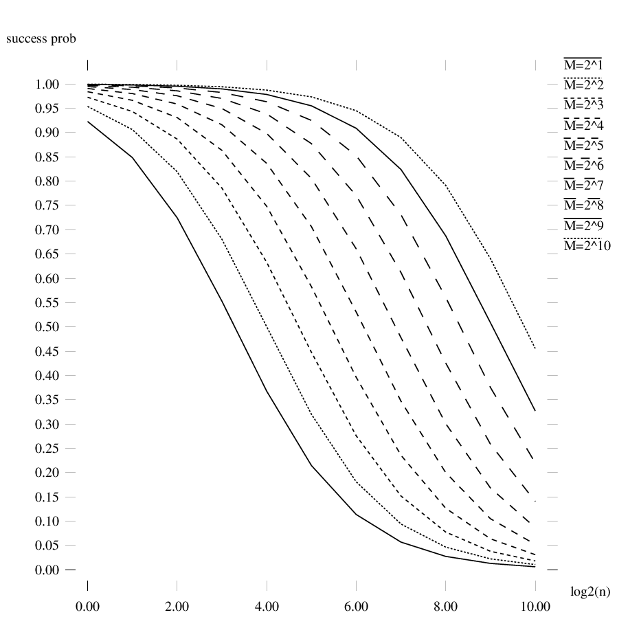
Refer to caption — Figure 1. The effect of doubling $M$ on the success probability

Remark 2.2.

According to Approximation (3), in order to maintain the success probability when $m$ is doubled, $M$ should be multiplied by $2^{1.7165/0.5437}\approx 8.92$ .

Another interpretation is as follows. Assume that we wish to decide what should the value of $M$ be to get success probability $0.5$ , that is, $L=0$ . From (3) it follows that

x_{5}\approx(-7.0814+1.7165x_{1}+0.7547x_{2}-0.1094x_{3})/0.5437

and therefore

M=2^{x_{5}}\approx 0.00012\cdot m^{3.16}\cdot n^{1.39}/k^{0.2}.

It seems that the prediction capabilities of Approximation (3) for larger parameters are not bad.

Example 2.3.

Using Approximation (3), the predicted success probability for parameters list $(16,128,8,8,1024)$ is $0.668$ . An experiment for these parameters succeeded in $9$ out of $11$ tries (about $0.82$ ).

2.1. Identifying failures

Figure 2 describes the position of the correct prefix of $X$ and the average score of all $M$ sequences in the memory during the steps of the algorithm (The graphs are normalized for graphical clarity). Two typical examples are given, both for parameters list $(2,64,8,8,128)$ . An interesting observation is that when the correct prefix is not among the first few, the average length decreases more slowly with the steps of the algorithms.

It turns out that in most of the cases where the correct prefix of $X$ does not survive a certain step (that is, it is not ranked among the first $M$ sequences), the average length after several more steps almost does not decrease. Figure 3 illustrates two typical cases, with parameters list $(2,64,8,8,16)$ (left) and $(2,64,8,8,8)$ (right).

This allows us to identify failures within several steps after their occurrence. In such cases one approach is to return a few steps backwards, increase $M$ for the next (problematic) few steps, and then decrease it again.

We must stress that these are only typical cases, and several pathological cases (where the correlation between the decrease in the lengths and the position of the correct prefix was not as expected) were also encountered. In these rare cases, we observed at least one of the following phenomena: Either the generators $a_{i}$ could be written as a product of very few Artin generators, due to several cancellations in the product defining them (recall that each generator $a_{i}$ is a product of $10$ random Artin generators in $B_{8}$ ), or else some (but not all) of the Artin generators multiplied to obtain $a_{i}$ were cancelled when multiplied with some of the Artin generators defining $a_{j}$ (or its inverse), so that the resulting element $x$ could be written using much fewer Artin generators than expected. This violates the required monotonicity of the length function and makes the algorithm fail.

2.2. Working in $B_{N}$ when $N$ is larger

For the parameters lists $(2,16,8,8,2)$ and $(8,16,8,8,128)$ , we have checked the success probabilities for $N=8$ , $10$ , $12$ , $14$ , $16$ , $20$ , $24$ , $28$ , $32$ , $36$ , $40$ , $50$ , $60$ , $70$ , $80$ , $96$ , and $100$ . The results are shown in Figure 4. While the success probability decreases with $N$ , it does not become as negligible as one might expect. Moreover, it can be significantly enlarged at the cost of increasing $M$ .

3. Concluding remarks

Our results suggest that whenever $G$ is a finitely generated subgroup of the braid group, which is obtained by a sufficiently “random” process, and the involved parameters are feasible for handling the group elements in the computer, it is possible to solve equations in the given group with significant success probabilities. This significantly extends similar results concerning the conjugacy problem (with known parameters) obtained in other works (e.g., [5]).

This approach seems to imply the vulnerability of the key exchange protocols suggested in [1, 7], since their security is based on the difficulty of the Conjugacy Problem in “random” subgroups of the braid group (see Example 1.2). It should be stressed that our experiments were performed with a small amount of memory (parameter $M$ ), which could, in feasible settings, be increased by several orders of magnitude and therefore significantly improve the success probability. Since even a small non-negligible success probability in attacking the protocol implies that it is not secure, it seems that in order to immune the current protocols against the attack implied by the results here, the working parameters have to be increased so much that the system will become impractical.

However, in order to use our approach against newly proposed protocols based on the braid group (see [4]), or against similar protocols based on other finitely generated groups, one must first find a good length function for the specific problem.

References

[1] I. Anshel, M. Anshel and D. Goldfeld, An algebraic method for public-key cryptography, Math. Res. Lett. 6 (1999), 287–291.
[2] D. Garber, S. Kaplan, M. Teicher, B. Tsaban, and U. Vishne, Length-based conjugacy search in the Braid group, Contemporary Mathematics 418 (2006), 75–87.
[3] F. A. Garside, The braid group and other groups, Quart. J. Math. Oxford Ser. (2) 78 (1969), 235–254.
[4] Helger Lipmaa, Cryptography and Braid Groups homepage,
http://www.tcs.hut.fi/~helger/crypto/link/public/braid/
[5] D. Hofheinz and R. Steinwandt, A Practical Attack on Some Braid Group Based Cryptographic Primitives, PKC 2003 Proceedings, Lecture Notes in Computer Sciene 2567 (2003), 187–198.
[6] J. Hughes and A. Tannenbaum, Length-based attacks for certain group based encryption rewriting systems, Workshop SECI02 Sécurité de la Communication sur Internet, Tunis, Tunisa, September 2002.
[7] K. H. Ko, S. J. Lee, J. H. Cheon, J. W. Han, S. J. Kang and C. S. Park, New Public-key Cryptosystem using Braid Groups, CRYPTO 2000, LNCS 1880 (2000), 166–183.