Classification of Ding’s Schubert varieties: finer rook equivalenceThanks: This work was completed while the first author was visiting the Univeristy of Minnesota. First author supported by the American Institute of Mathematics. Second author partially supported by an NSF Postdoctoral Fellowship. Third author partially supported by NSF grant DMS–0245379
Abstract.
K. Ding studied a class of Schubert varieties in type A partial flag manifolds, indexed by integer partitions and in bijection with dominant permutations. He observed that the Schubert cell structure of is indexed by maximal rook placements on the Ferrers board , and that the integral cohomology groups , are additively isomorphic exactly when the Ferrers boards satisfy the combinatorial condition of rook-equivalence.
We classify the varieties up to isomorphism, distinguishing them by their graded cohomology rings with integer coefficients. The crux of our approach is studying the nilpotence orders of linear forms in the cohomology ring.
Key words and phrases:
Schubert variety, rook placement, Ferrers board, flag manifold, cohomology ring, nilpotence2000 Mathematics Subject Classification
Primary 14M15; Secondary 05E051. Introduction
The goal of this paper is to classify up to isomorphism a certain class of Schubert varieties within partial flag manifolds of type . Although this is partly motivated as a first step toward the isomorphism classification of all Schubert varieties, we choose here to explain instead our original motivation, stemming from rook theory in combinatorics.
A board is a subset of the squares on an chessboard, and a -rook placement on is a subset of squares in , no two in a single row or column. Kaplansky and Riordan [9] considered the problem of when two boards are rook-equivalent, that is, when for each , the number of -rook placements is the same as .
Foata and Schützenberger [4] solved the problem for the well-behaved subclass of Ferrers boards ; these are the usual Ferrers diagrams associated to partitions11 1 NB: we are writing our partitions with the parts in weakly increasing order, contrary to usual combinatorial conventions, but more convenient in this setting.
| (1) |
having all squares left-justified in their row, with squares in the bottom row, in the next, etc. They showed that each rook-equivalence class of Ferrers boards has a unique representative which is a strict partition, i.e., satisfying . Goldman, Joichi and White [8] re-proved this result by showing that and are rook-equivalent if and only if the multisets of integers and coincide.
Garsia and Remmel [6] defined -rook polynomials that -count the -rook placements on by a certain “inversion” statistic generalizing inversions of permutations. They also showed that the problem of -rook equivalence is the same as that of rook equivalence. When for each , this can be deduced from a product formula for that counts placements of rooks: up to a factor of it is
| (2) |
where .
K. Ding [2, 3] interpreted this product as the Poincaré series for a certain algebraic variety which he called a partition variety. Fix a standard complete flag of subspaces
and define
| (3) |
The set may be endowed with the structure of a smooth complex projective variety, and (although not stated explicitly in [2]) is in fact a smooth Schubert variety inside the partial flag manifold , where denotes the rectangular board with rows and columns. As we shall explain below, the Schubert varieties arising in this way are (in the notation of [5, §10.2]) those of the form , where is a 312-avoiding permutation. Equivalently, the fundamental cohomology class is represented by a Schubert polynomial indexed by a dominant or 132-avoiding permutation. (See [5] for a reference on Schubert varieties, and [10] for a detailed treatment of Schubert polynomials.) Ding observed that the Schubert cell structure inherited by has cells indexed by -rook placements on , and with the dimension of the cell governed by Garsia and Remmel’s inversion statistic. Since these cells are all even-dimensional, their (co)homology is free abelian, occurring only in even dimension, and the Poincaré series of is given by the -rook polynomial formula (2). From this Ding concluded [3] that two partition varieties have additively isomorphic (co)homology groups if and only if and are rook-equivalent.
It is natural to ask when two such Ding partition varieties have isomorphic (graded) cohomology rings, or even when they are isomorphic as varieties. The main result of this paper is that the answers to both questions are the same. We make use of recent results of Gasharov and the third author [7], giving simple explicit cohomology ring presentations22 2 It is amusing that these cohomology ring presentations for Schubert varieties are often derived for the purposes of enumerative geometry (Schubert calculus), but are used here for a different classical topological purpose, namely distinguishing non-homeomorphic spaces. for a more general class of Schubert varieties in partial flag manifolds (those defined by a conjunction of inclusion conditions of the forms and ).
To state our main result, we first note one trivial source of isomorphisms among the partition varieties . We assume throughout that for every , for otherwise . However, if for some , then the condition with forces , so that is isomorphic to , where
Here if , so that , there is no partition and we simply note that .
Say that is decomposable if this occurs (i.e., if for some ), and indecomposable otherwise. For example, the partition shown in Figure 1 is decomposable since . In this case, one has and , as shown in the figure.
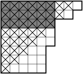
Iterating this, one can decompose into a multiset of indecomposable partitions , which we will call its indecomposable components, such that
| (4) |
Our main result is that the Schubert varieties are determined up to isomorphism by these multisets of indecomposable components. It should be compared with the result of Goldman, Joichi and White [8], which can now be rephrased: the varieties are determined up to additive (co-)homology isomorphism by the multisets of numbers .
Theorem 1.1.
The following are equivalent for two partitions, and :
- (i)
The multisets of indecomposable components, and , are identical.
- (ii)
There is an isomorphism of varieties.
- (iii)
There is a graded isomorphism of integer cohomology rings .
The implications (i) (ii) (iii) are clear; the hard part is to show that (iii) implies (i). It turns out that the key to this implication lies in understanding the nilpotence orders of cohomology elements ; that is, the least for which .
In Section 2, we review some of Ding’s results, and re-prove somewhat more directly the presentation for from [7]. The three sections that follow are the technical heart of the paper, categorizing elements in of minimal nilpotence order. We begin in Section 3 by setting up some Gröbner basis machinery that we shall use throughout (for a general reference on Gröbner basis theory, see [1]). Section 4 deals with nilpotents in the cohomology of the complete flag variety (that is, when is a square Ferrers board) and Section 5 treats the case of arbitrary . Using these tools, we prove in Section 6 that an indecomposable partition may be recovered from the structure of as a graded -algebra. Finally, in Section 7, we show that in the general case, has an essentially unique decomposition as a tensor product of graded -algebras, whose factors correspond to the indecomposable components of the partition .
It is curious that this unique tensor decomposition fails if instead of the integer cohomology ring one takes cohomology with coefficients in a ring where is invertible; see Remark 7.6 below.
2. Review of and the presentation of
For the sake of completeness, and also to collect facts for future use, we begin by re-proving some of Ding’s results from [2], and re-derive somewhat more directly the presentation given in [7] for the cohomology ring of . Throughout this paper, all cohomology groups and rings are taken with integer coefficients unless otherwise specified. We begin by identifying the Schubert varieties that arise as Ding’s varieties . (See [5, §10.6] for more information on Schubert varieties, and [10] for a detailed treatment of Schubert polynomials.)
Let be the symmetric group of permutations of , and let be the subgroup of permutations fixing pointwise. Consider the partial flag variety
Let be a permutation which is a maximum-length representative for its coset in . The corresponding Schubert variety is defined to be
Let be a partition of the form (1), and let . It is easy to check that Ding’s variety coincides with the Schubert variety , where is the unique permutation given by the recursive rule
Note that if , then corresponds to the maximal rook placement on the Ferrers board given by the following algorithm: let increase from to , and for each , place a rook in row and column , where is the rightmost square in row whose column does not already contain a rook. For instance, if , then . (If , then we must first augment with additional rows of length .) It is not hard to verify that the permutations obtained in this way are exactly those which are 312-avoiding; that is, there do not exist for which and . Equivalently, the cohomology class is represented by a Schubert polynomial which is a single monomial, namely the Schubert polynomial indexed by the dominant (or 132-avoiding) permutation , where is the unique permutation of maximal length. (We thank Ezra Miller for discussions clarifying these points.)
Because is a Schubert variety, it comes equipped with a Schubert cell decomposition, having cells in only even real dimensions. As observed by Ding, this has important consequences:
Theorem 2.1 (Ding [2]).
The integral cohomology ring is free abelian (that is, it has no torsion), is nonzero only in even homological degrees, and has Poincaré series
Proof.
The cohomology is free abelian and concentrated in even degrees because the Schubert cell decomposition for the Schubert variety has cells only in even dimensions.
For the assertion about the Poincaré series, we will induct on . The map
is an (algebraic) fiber bundle, with fiber isomorphic to , where
is the partition obtained by removing the first row and column from (see Figure 2).
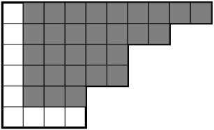
The Leray-Serre spectral sequence is particularly simple in this situation, because both base and fiber are simply-connected (again due to the Schubert cell decomposition) and have homology concentrated in even dimension. This causes the spectral sequence to degenerate at the -page, yielding
The assertion about now follows by induction on , using the fact that . ∎
We now set about deriving the presentation for . To this end, we recall Borel’s picture for the cohomology of the complete flag manifold and the partial flag manifold ; see [5, Chapter 10, §3, §6]. We will use the following notation for symmetric functions in various sets of variables. For integers and , define the elementary and complete homogeneous symmetric functions, respectively, by
| where | ||||
According to Borel’s picture, , where is the ideal generated by all symmetric functions of positive degree, and where represents the negative of , the first Chern class of the line bundle on whose fiber over the flag is .
Furthermore, the surjection which forgets the subspaces of dimension greater than in a complete flag induces a map which turns out to be injective, and the image of is identified with the invariant subring . This invariant subring may be presented as , where
and is the ideal of with the same generators as .
The relations in the ideals and induce further relations among various symmetric functions, which we record here for future use.
Proposition 2.2 (cf. [5, p. 163, eqn. (4)]).
For every and , one has
Proof.
Hence
Now comparing coefficients of powers of yields the desired equality. ∎
We now give the general presentation for the integral cohomology of (as pointed out in [7, Remark 3.3]).
Theorem 2.3.
Let be a partition with and for all . Let
where .
Then there is a (grade-doubling) ring isomorphism
sending to . Here is the same line bundle as above, but restricted to from the partial flag manifold .
Proof.
The obvious inclusion induces a map . This ring map is surjective, because inherits from a decomposition into Schubert cells, and the dual cocycles to these (even-dimensional) cells additively generate the cohomology in each case.
There are further relations on the Chern classes in due to the conditions . Specifically, the bundle on will have the same Chern classes as the direct sum , in which is a trivial bundle. Thus when restricted to , the bundle will have the same Chern classes as the bundle of rank . Hence its Chern classes for inside must vanish. Consequently, we have a surjection of rings
| (5) |
where
We now manipulate the quotient ring on the left of (5). We use Proposition 2.2 to draw two conclusions:
- (i)
Applying Proposition 2.2 with shows that and are generated as algebras by , since their generators of the form can be expressed modulo as (symmetric) polynomials in .
- (ii)
Applying it with for shows that in , because for each , is congruent modulo to .
Consequently, there is a surjection of rings
| (6) |
On the other hand, the set
is a Gröbner basis for with respect to the lexicographic term order on given by . Indeed, the initial term of is , so these generators have pairwise relatively prime, monic initial terms. Consequently, the quotient ring on the left of (6) is a free -module of rank , with -basis given by the standard monomials (those divisible by none of the initial terms), namely . Since Theorem 2.1 implies that is a free -module of the same rank, the surjection (6) must be an isomorphism. ∎
For example, if is the partition shown in Figure 1, then the Gröbner basis for is
The previous proof shows that is the elimination ideal
This observation has some useful corollaries, which can also be proved by direct combinatorial/algebraic arguments avoiding any use of geometry. The first corollary is the algebraic manifestation of the (surjective) map induced by the inclusion of Schubert varieties .
Corollary 2.4.
Let and be partitions, both with nonzero rows, such that .
Then , and consequently, is a quotient of .
Proof.
By definition of , one has in this situation. ∎
Corollary 2.5.
If for some then the ideal is invariant under permutations of the variables .
Proof.
It suffices to show that has this same invariance. Note that the generators for of the form
are all redundant, as they lie in the ideal generated by . The latter generators, and all other generators of , are symmetric in . ∎
3. Two reduced Gröbner bases
This section examines the Gröbner bases for for two extreme cases of indecomposable partitions. In both cases, one can describe the (unique) reduced Gröbner basis, which will be used in an essential way later in the paper. We assume some familiarity with “Gröbner basics” on the reader’s part; a good reference for this topic is [1].
We begin with some notation regarding Gröbner reduction. Since the generators form a Gröbner basis for with respect to a lexicographic monomial ordering in which , we can compute in the quotient by reducing polynomials modulo this Gröbner basis. For a polynomial , we will denote by this standard form of . That is, is the unique -linear combination of standard monomials which is congruent to modulo . Given a standard monomial , we denote by the coefficient of in . (This is well-defined, because the standard monomials form a basis for as a free -module.)
Let and for some fixed , let . Then the fact that we are using a lexicographic order to perform reductions has the following easy consequence (see also [1, §3.1]), which will be used frequently. It can be viewed as an algebraic consequence of the fibration that forgets the subspaces of dimension greater than in a flag, which happens to induce an injective map .
Proposition 3.1.
Let and be related as above. Suppose that in lies in some subalgebra , where .
Then the images of in and have the same standard form .
Our first extreme case arises when is an indecomposable partition with , and is the smallest indecomposable partition having , namely .
Proposition 3.2.
Let . With respect to lexicographic order on with , the ideal has reduced Gröbner basis
| (7) |
Proof.
It is easy to see that the elements of (7) form a reduced Gröbner basis with respect to the lexicographic order for whatever ideal they generate. We observe that this ideal may also be presented as
We will show that this ideal is exactly . By Theorem 2.3,
so it remains only to show that and are congruent modulo the ideal . Since , this congruence is immediate from the fact that
which is easily proven by double induction on and via the identity . ∎
Our second extreme case arises when is an indecomposable partition with rows. Let , and let be the smallest indecomposable partition with rows and . That is,
| (8) | ||||
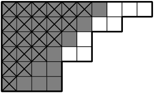
Then is a subpartition33 3 For the purposes of this paper, the statement “ is a subpartition of ” means that for all rows of . Equivalently, the Ferrers diagram of is contained inside that of , when both are left- and bottom-justified. of , which we will call the core of . For example, the core of is the partition (see Figure 3).
Proposition 3.3.
For , let be a partition which is its own core.
Then the polynomials
| (9) | ||||||||||
form a reduced Gröbner basis for under the reverse lexicographic term order given by .
Proof.
The initial terms of the ’s are (in order) , , …, , , …, . It is evident that no initial term divides any term of any other . Therefore, they are a reduced Gröbner basis for the ideal that they generate.
We claim that for every ,
The claim is trivial for . For , it follows from induction and the observation that . In particular, the equality for gives . ∎
The form of this reduced Gröbner basis has the following consequence, which we will exploit later.
Corollary 3.4.
(“Stickiness”) Let be an indecomposable partition which is its own core, and . Let be a monomial in .
Then:
- (1)
If and is divisible by , then so is .
- (2)
If is not divisible by any of the variables , then neither is .
Proof.
(1) is immediate from the previous discussion. For (2), the only Gröbner basis elements that can be used in the reduction of are , so the reduction process cannot introduce a monomial divisible by any of . ∎
One useful consequence of “stickiness” is the following.
Corollary 3.5.
Let be an indecomposable partition which is its own core, and . Let be an element of the degree-one graded piece of . Decompose as , where
If in for some positive integer , then in .
Proof.
Note that , where is some polynomial divisible by . Passing to the standard forms, we find that . By Corollary 3.4, no monomial in is divisible by a sticky variable (that is, one of ), but every monomial in is divisible by a sticky variable. Therefore (). ∎
4. Nilpotence of linear forms in the cohomology of
The main result of this section, Theorem 4.1, concerns the nilpotence orders of degree- elements in the graded ring . This result may be of independent interest, and it would be nice to have a geometric explanation for it.
Recall that , where
| (10) |
We digress to discuss graded -algebras and nilpotence. A standard graded -algebra is a ring with a -module direct sum decomposition in which each is a free -module, and is generated over the subalgebra by . Let be a ring and a nilpotent element (that is, some power of is zero). The nilpotence order of is defined as the smallest integer such that ; we will sometimes say that is -nilpotent. (So has nilpotence order 1 if and only if .)
By Theorem 2.3, is a standard graded -algebra, with . Furthermore, every element of is nilpotent, since has finite rank as a -module. The nilpotence order of these linear forms will be our main tool in distinguishing the rings . In this section, we study the case that ; we treat the general case in Section 5.
Note that the images of the variables in satisfy . Indeed, by Corollary 2.5, it is sufficient to prove that , which follows from (10) since contains the element . In fact, more is true:
Theorem 4.1.
Let .
Then has nilpotence order greater than or equal to , with equality if and only if is congruent, modulo , to a scalar multiple of one of the variables .
We first show that is the minimal nilpotence order achieved by any linear form.
Proposition 4.2.
Let be a linear form. If , then .
Proof.
Let be a preimage of under the quotient map . Then means . By degree considerations, this means that belongs to the ideal
| (11) |
Thus it suffices to show that is a radical ideal, since then and in . We will show something slightly stronger: that the ideal is radical. Indeed, any nonzero nilpotent in would give rise to a nonzero nilpotent in .
Let be a primitive root of unity. We claim that is the vanishing ideal for the variety , defined as the union of all lines whose slope vector is any permutation of . Note that there are exactly such lines, because two such slope vectors that differ by multiplication by a root of unity give rise to the same line. Equating coefficients of powers of in the equation
shows that . For the reverse inclusion, note that is a regular sequence in , and therefore cuts out scheme-theoretically a complete intersection of Krull dimension , that is, a set of curves with various multiplicities. By Bézout’s Theorem, the sum of the degrees of those curves, counted with multiplicities, must be
But this complete intersection contains at least lines in , each of degree . Therefore it contains no other curves, and each line occurs with multiplicity 1; that is, . ∎
To complete the proof of Theorem 4.1, we must show that the scalar multiples of the variables are the only -nilpotent linear forms in . In what follows, we regard a linear form as a -linear functional, mapping to .
Lemma 4.3.
Let , with , and let be a nonzero constant. Suppose that for all whose coordinates are permutations of the distinct roots of unity.
Then for some .
Proof.
Let be a primitive root of unity. Let the symmetric group act on by permuting coordinates, and for a permutation , abbreviate by . Replacing with , we may assume that for all . That has the desired form is equivalent to the statement that at least of the coefficients are equal. This is trivial if or , and can be checked by direct calculation if . Therefore, suppose . By transitivity, it suffices to show that if two coefficients are different, then the other are mutually equal.
Suppose that . Choose so as to maximize , and let such that and . Then and are both roots of unity, and
| (12) |
Taking the magnitude of both sides, the choice of and implies that . On the other hand, if we choose to minimize , the same argument implies that . We conclude that .
Note that and are the only roots of unity whose difference is . (This may be seen most easily by plotting the roots of unity in the complex plane, and observing that no two of the line segments joining two maximally distant roots are parallel.) Therefore, the equation (12) implies that the values and do not depend on . Hence as desired. ∎
Proposition 4.4.
Let be a linear form such that .
Then for some .
Proof.
Let be a preimage of under the quotient map ; that is, . By degree considerations, there is a constant such that modulo . As in the proof of Proposition 4.2, the ideal vanishes on all vectors whose coordinates are a permutation of the distinct roots of unity. Therefore for all such vectors . By Lemma 4.3, there is some such that . As , this implies . Consequently in . This completes the proof of the proposition and of Theorem 4.1. ∎
5. Nilpotence of linear forms in the cohomology of
Throughout this section, will be an indecomposable partition. We continue our study of nilpotence orders of linear forms in the graded -algebra . The main result is the following classification of linear forms of minimal nilpotence order, generalizing Theorem 4.1.
Theorem 5.1.
Let be an indecomposable partition, and let . Then is the minimal nilpotence order of any linear form in . Moreover, if has exactly parts equal to (that is, ), then the elements of of nilpotence order exactly are classified as follows:
- Case I.
Either , or .
Then the -nilpotents in are the multiples of .
- Case II.
(that is, ).
- Subcase IIa.
Either , or is odd.
Then the -nilpotents are , and .
- Subcase IIb.
Both and is even.
Then the -nilpotents are , , and .
- Subcase IIa.
By way of motivation for the rather technical matter of this section, we explain how the classification of nilpotents will be used in the next two sections to recover a partition from its cohomology ring. Theorem 5.1 implies immediately that is an isomorphism invariant of . Moreover, by the presentation of Theorem 2.3, the quotient ring may be identified with the ring , where is the partition obtained by removing the first row and column from (see Figure 2). However, it is really necessary to describe as a quotient , where is some linear form identified intrinsically from the structure of as a standard graded -algebra, that is, in a way that does not depend on the presentation. The classification of nilpotents in Theorem 5.1 is the tool that allows this. It turns out that we will require almost all, but not quite all of the last assertion in the theorem, so we only prove the parts that will be used. (The arguments we omit are very similar to those that we include.)
In the first part of this section, culminating in Proposition 5.4, we prove the first assertion of Theorem 5.1, namely that is the minimal nilpotence order of any linear form in . We begin with a weaker statement: that no linear form in the first variables has nilpotence order less than .
Lemma 5.2.
Let be indecomposable with . Let ; that is, is supported only on the first variables. Then, in ,
- (a)
if and only if , and
- (b)
if , then is a scalar multiple of one of the following: .
Proof.
By Proposition 3.1 and the hypothesis that is supported only on the first variables, we may assume without loss of generality that . By Corollary 2.4, we may decrease the part sizes of (if necessary), so as to assume that . But then using Proposition 3.1 again, we can re-introduce parts all of size , and work in the ring , where assertion (a) follows from Theorem 4.1.
In fact, assertion (b) also follows from Theorem 4.1. The degree- graded piece of is generated by , so the elements of listed above are the only ones that are congruent modulo to a scalar multiple of a variable (here we use the fact that ). ∎
An immediate consequence of Lemma 5.2 is that every linear form of nilpotence order must be supported on at least one of the variables . This is where the concept of “stickiness” introduced in Corollary 3.4 first comes into play.
Proposition 5.3.
Let be indecomposable with , and let . Then if and only if in .
Proof.
Assume , but in . By Lemma 5.2(a), we may assume . By Proposition 3.1, we may assume without loss of generality that is its own core.
Writing , where and , it follows from Corollary 3.5 that . Hence by Lemma 5.2. That is, . If is not supported on (that is, ), then we may replace with the partition obtained by removing the th (largest) row. Repeating this as many times as necessary, we may assume without loss of generality that .
Now let be any monomial in the variables . Note that
| (13) |
because the variables are sticky (Corollary 3.4). Reducing using the Gröbner basis element of (9), we find that
| (14) | ||||
where . Combining this with (13) yields
| (15a) | |||||
| (15b) | |||||
where (15a) follows from stickiness, and (15b) from the fact that only are used in reducing (15a).
The polynomial is nonzero in since is indecomposable. Thus Lemma 5.2 implies that as well, and so there exists some monomial in the variables for which . Note that is also a standard monomial for . Therefore , a contradiction. ∎
Proposition 5.4.
When is indecomposable, the number is an isomorphism invariant of as a graded ring: namely, it is the minimum nilpotence order achieved by any linear form.
Proof.
Proposition 5.3 states that no nonzero linear form can have nilpotence order strictly less than . On the other hand, has nilpotence order at most , because . ∎
In the second part of this section, we show that the various linear forms mentioned in Theorem 5.1 are the only possible -nilpotents in . We begin by determining the nilpotence order of each variable.
Proposition 5.5.
When is indecomposable, the variable is -nilpotent in .
Proof.
Let . First, we show that in . Let be the partition given by
Then is a subpartition of , so is a quotient of by Lemma 2.4. It suffices to show that in , which follows from Corollary 2.5 since .
It remains to show that in . By Proposition 3.1 and Corollary 2.4, it suffices to show that in , where is the subpartition of given by
Note that is indecomposable, and that has a reduced Gröbner basis given by (7). A Gröbner reduction similar to (14), using the Gröbner basis element yields the equation
Since further reductions modulo can only involve the other generators , we may conclude that in , provided that in . Using the fact that , this follows from the following more general assertion: for any and ,
| (16) |
This is trivially true for . For , we prove it by induction on :
This last expression follows from using to perform repeated Gröbner reduction on each summand. By induction, , so we obtain
establishing (16) as desired. ∎
Proposition 5.6.
Let . Suppose that .
Then is a scalar multiple of one of the following:
| (17) | ||||
The last case can occur only if is even.
Proof.
By Corollary 2.4, we may replace with its core. Let be the part of in the non-sticky variables. Then by Corollary 3.5. By Lemma 5.2(b), is either zero or of the form for some , or , where is a nonzero scalar. Without loss of generality, we may assume that .
If then we are done. Otherwise, we must show that is a scalar multiple of , and is even. By Proposition 3.1, we may assume without loss of generality that involves the variable with non-zero coefficient; that is,
where and is a linear form in the variables . We consider in turn each of the three possibilities: namely, , , or .
Case 1: .
We will rule out this case by deriving a contradiction from the assumption that in . Taking the further quotient of by the variables , one obtains a ring isomorphic to , where
is an indecomposable partition, with parts, equal to its own core. If in , then in . So in (because ). But this contradicts Corollary 5.5, since .
Case 2: , where .
Assume that (the case falls under Case 3 below). As in Case 1, we wish to reach a contradiction. Consider the quotient ring
which is isomorphic to . Let be the image of in ; then . By Theorem 4.1, must be a scalar multiple of some variable. This is possible only if and ; that is, is a scalar multiple of either or . All that remains is to check that neither nor belongs to the ideal ; this is a routine calculation. Thus in all cases, a contradiction. Case 2 is therefore ruled out.
Case 3: .
Let be any standard monomial for of degree in the non-sticky variables ; then is also standard. Using stickiness of the variables and the fact that , we have for every such monomial
This last expression must be zero since in . On the other hand, in , so there is at least one such monomial in for which . It follows that . Since , the only possibility is that is even and . If , then we are done; we need to rule out the case .
Suppose that . Replacing with in the above calculation, we find that the coefficient is either 0 or 2. Bearing in mind that , we pass to the quotient ring
Note that since equals either or , and in , the image of in is of the form . Since and are both zero in , we have
But in by Theorem 4.1, so in . Hence in , which implies that in , as desired. ∎
We now know that every -nilpotent linear form in is, up to scalar multiplication, one of the linear forms (17). However, if is not its own core, then we must consider the possibility that one or more of these linear forms actually has nilpotence order strictly greater than . We examine each candidate in turn; Proposition 5.5 immediately takes care of the possible nilpotents .
Proposition 5.7.
Let be indecomposable with parts and . Let .
Then if and only if .
Proof.
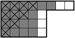
By Corollary 2.4, it will suffice to show that in . We may rewrite the presentation of as
using the fact that
Therefore for all . Letting , so that , we have in
No further Gröbner reduction is possible, so is zero if and only if , , and are all zero. But , and by Proposition 5.3. We conclude that in as desired. ∎
For the remaining assertions of Theorem 5.1, we are left only to consider the potentially -nilpotent linear form . Rather than determining exactly when is -nilpotent as in the theorem (which can be done by an argument similar to Proposition 5.7), we content ourselves with checking directly the case , since this is all we need for the present study. Here , and by Proposition 3.1) we may work in the ring
Then it is easily seen that is zero in this ring if and only if .
6. The indecomposable case
We now use the results of the previous section to prove that an indecomposable partition is determined uniquely by the cohomology ring of the corresponding Schubert variety.
Theorem 6.1.
Every indecomposable partition may be recovered from the structure of the ring as a graded -algebra. In particular, if and are different indecomposable partitions, then and are not isomorphic.
Proof.
We induct on , the number of parts of . Since is indecomposable, is the rank of as a free -module. By Theorem 5.1, the smallest part is the minimal nilpotence order of any member of . Moreover, as mentioned at the beginning of Section 5, , where is obtained from by deleting the first row and column (see Figure 2). By induction, it suffices to show that we can describe up to isomorphism in a way that is independent of the presentation.
We proceed by examining the same two cases as in Theorem 5.1; however, we subdivide Case II slightly differently into subcases.
Case I. or .
Let be the greatest index such that . Then Theorem 5.1 tells us that the -nilpotent linear forms in are (up to -multiples) . Consequently, up to sign, these are exactly the primitive -nilpotents, that is, those -nilpotents which can only be expressed as a scalar multiple for another -nilpotent and if .
By Corollary 2.5, one has () for every , and hence may be identified intrinsically as the quotient of by an arbitrary primitive -nilpotent linear form.
Case II. .
Then the primitive -nilpotents are (up to sign) , and if is even, possibly also .
Subcase IIA. .
If is odd, then the “extraneous” primitive -nilpotent is absent. If is even, then is distinguished intrinsically as the unique primitive -nilpotent which is -linearly independent of all the others.
Thus, in all cases when , we can intrinsically identify the primitive -nilpotents , , , , up to sign. By Corollary 2.5, the first forms on this list all have . Hence can be identified intrinsically by “majority rule”: it is the -algebra that occurs (up to isomorphism) as the quotient of by at least of the different primitive -nilpotent linear forms (other than the one, namely , that is linearly independent from the rest, as above). Note that the fact that out of is a well-defined “majority” uses the assumption that .
Subcase IIB. .
If , then is the unique primitive -nilpotent up to sign, so it is distinguished intrinsically, as is .
If , then there are two primitive -nilpotents up to sign, namely and . We claim that the graded -algebra map defined by
is an automorphism of interchanging with . Indeed, it is a routine calculation to check that lifts to an automorphism of , and that . In particular, may again be described up to isomorphism as the quotient of by an arbitrary primitive -nilpotent linear form. ∎
7. The decomposable case
We now consider the case that is decomposable, with indecomposable components . In this case, . Since each has no torsion in its (co-)homology by Theorem 2.1, the Künneth formula [11, §61] implies a tensor decomposition for the associated cohomology rings:
| (18) |
Together with the uniqueness result for indecomposable partitions (Theorem 6.1), it would seem that we are done. However, there is one remaining technical point: to verify that the partitions can be read off intrinsically from the structure of as a graded -algebra, we must check that the tensor decomposition (18) is unique.
To do this, we make further use of the facts about nilpotence established in Section 5. But first we must make precise the notion of tensor decomposition, and point out how it interacts with order of nilpotence.
For a standard graded -algebra, a tensor decomposition is an isomorphism of graded -algebras in which each is a standard graded -algebra. Note that any such decomposition is completely determined by the associated direct sum decomposition of free -modules , since is then the subalgebra of generated by the direct summand of . Say that a tensor decomposition of is nontrivial if for all . Say is tensor-indecomposable if it is not itself, and has no nontrivial tensor decomposition.
Lemma 7.1.
Suppose that . Let ; that is,
where . Let be the nilpotence order of . (Recall that if and only if .)
Then the nilpotence order of is
Proof.
By the pigeonhole principle, each term of the multinomial expansion of is divisible by for some ; therefore, in . For the same reason, all but one term of the multinomial expansion of vanishes; the exception is
which is nonzero, since it is nonzero in each tensor factor. ∎
This calculation has immediate useful consequences.
Corollary 7.2.
Let be a standard graded -algebra with a nontrivial tensor decomposition . Then any linear form that achieves the minimal nilpotence among all elements in must lie in for some .
Corollary 7.3.
Let be a partition with indecomposable components . If corresponds to in this decomposition, then is -nilpotent in .
For example, if is the decomposable partition shown in Figure 1, then correspond to the rows of , and to the rows of . Thus the variables have nilpotence orders , respectively, in (and in ), and have nilpotence orders and , respectively. (Note that these seven variables are a -basis for ; does not correspond to a variable in the presentation for .)
Proposition 7.4.
Let be an indecomposable partition. Then the ring is tensor-indecomposable.
Proof.
Let denote the number of parts in , and its smallest part. We proceed by induction on .
If , then clearly is indecomposable. Otherwise, suppose that is a nontrivial tensor decomposition; we will obtain a contradiction.
By Proposition 5.4, is a nilpotent of minimal order, and hence by Corollary 7.2, without loss of generality, . Then . On the other hand, , where is the partition obtained from by removing the first row and column. Since is indecomposable, so is . By the inductive hypothesis, the decomposition must be trivial; that is, , and must be generated by as a -algebra, i.e., . Therefore, exactly one member of the set
belongs to . Let be the nilpotence order of that one form; then all other elements of have nilpotence order by Lemma 7.1. Let ; note that since is indecomposable. By Proposition 3.1 we can work in the algebra , namely the quotient of by the ideal
Let be arbitrary. We will show that no linear form has nilpotence order strictly less than . Indeed,
This last expression is exactly the standard form of . For , the summand is ; since and is an integer, the coefficient is nonzero. Therefore .
On the other hand, in by Proposition 5.5. Therefore must be the unique element of with minimal nilpotence order , and every other element of must have nilpotence order . But there are no standard monomials in of degree greater than , which implies that every element of has nilpotence order or less. This contradiction completes the proof. ∎
We now establish the key fact of the decomposable case, that these decompositions are actually unique.
Lemma 7.5.
The ring has a unique tensor decomposition into tensor-indecomposables. Specifically, if has indecomposable components , then
is the unique tensor decomposition of , up to permuting the factors.
Proof.
The existence is immediate, since each is tensor-indecomposable by Lemma 7.4. For uniqueness, we proceed by induction on the number of rows of . If has only one row, the statement is trivial.
Suppose that is a tensor decomposition with each tensor-indecomposable, so that
| (19a) | ||||
| (19b) | ||||
Let be the minimal nilpotence order of any element of . Then by Corollary 7.3. Without loss of generality, we may re-index so that ; then is a linear form of nilpotence order . By Corollary 7.2, must belong to one of the , say . Let be the partitions obtained by removing the left column and bottom row of , respectively. Then
| (20a) | ||||
| (20b) | ||||
By induction, the rightmost expression in (20a) is the unique tensor decomposition of into tensor-indecomposables (possibly with a superfluous factor if has only one part). Thus the rightmost expression in (20b) is unique—clearly not as a direct sum decomposition of as a -module, but as a direct sum decomposition which induces a tensor decomposition of .
Now assume that has rows, so that generate as a -subalgebra of . For each , consider the image of in . Since each belongs to the direct summand on the left side of the unique decomposition (20b), it must belong either to , or to for some . On the other hand, Corollary 7.3 tells us that is -nilpotent in , but is -nilpotent in . That is, the nilpotence order of drops by in the quotient by (because ). If for some , then this last observation contradicts Lemma 7.1. Therefore , from which we conclude that .
Consequently, the uniqueness property of the decomposition (20b) implies that
for some subset . Since lies in both and , we conclude that
and, since is a standard graded -algebra,
But was assumed to be indecomposable, so this forces . Hence and . By the uniqueness property of (20b), we must have , and after re-indexing, for . Thus the two tensor decompositions in (19a) are identical. ∎
The nontrivial implication (iii) (i) in the main result, Theorem 1.1, is now immediate from Lemma 7.5 and Theorem 6.1.
Remark 7.6.
As we shall now demonstrate, it was essential to study the cohomology of with integer coefficients. If is a coefficient ring in which is invertible, then Proposition 7.4, Lemma 7.5 and Theorem 1.1 would all fail to hold if “graded -algebra” was replaced with “graded -algebras”. That is, Ding’s Schubert varieties are not classified up to isomorphism by their cohomology with -coefficients. For example, consider the indecomposable partition . By completing the square, one has
Thus indecomposable partitions do not lead to tensor-indecomposable graded -algebras. This also leads to “extra” isomorphisms among the cohomology rings . For example, the partition has indecomposable components . Since , one has
even though and do not have the same indecomposable partition components.
References
- [1] D. Cox, J. Little, and D. O’Shea, Ideals, varieties, and algorithms. An introduction to computational algebraic geometry and commutative algebra. Second edition. Undergraduate Texts in Mathematics, Springer-Verlag, New York, 1997.
- [2] K. Ding, Rook placements and cellular decompositions of partition varieties. Discrete Math. 170 (1997), 107-151.
- [3] K. Ding, Rook placements and classification of partition varieties , Commun. Contemp. Math. 3 (2001), 495–500.
- [4] D. Foata and M.-P. Schützenberger, On the rook polynomials of Ferrers relations. Combinatorial theory and its applications, II (Proc. Colloq., Balatonfüred, 1969), pp. 413–436. North-Holland, Amsterdam, 1970.
- [5] W. Fulton, Young tableaux. London Mathematical Society Student Texts 35. Cambridge University Press, Cambridge, 1997.
- [6] A.M. Garsia and J.B. Remmel, -counting rook configurations and a formula of Frobenius. J. Combin. Theory Ser. A 41 (1986), 246–275.
- [7] V. Gasharov and V. Reiner, Cohomology of smooth Schubert varieties in partial flag manifolds. J. London Math. Soc. 66 (2002), 550–562.
- [8] J.R. Goldman, J.T. Joichi, and D.E. White, Rook theory. I. Rook equivalence of Ferrers boards. Proc. Amer. Math. Soc. 52 (1975), 485–492.
- [9] I. Kaplansky and J. Riordan, The problem of the rooks and its applications. Duke Math. J. 13 (1946), 259–268.
- [10] I.G. Macdonald, Notes on Schubert polynomials. Publications du LACIM, Université du Québec à Montréal, 1991.
- [11] J.R. Munkres, Elements of algebraic topology. Addison-Wesley Publishing Company, Menlo Park, CA, 1984.