Finite-Element Discretization of Static Hamilton-Jacobi Equations Based on a Local Variational Principle

Folkmar Bornemann and Christian Rasch Address: Center of Mathematics, Technical University of Munich, 80290 Munich, Germany Email address: {bornemann,rasch}@ma.tum.de

Abstract.

We propose a linear finite-element discretization of Dirichlet problems for static Hamilton-Jacobi equations on unstructured triangulations. The discretization is based on simplified localized Dirichlet problems that are solved by a local variational principle. It generalizes several approaches known in the literature and allows for a simple and transparent convergence theory. In this paper the resulting system of nonlinear equations is solved by an adaptive Gauss–Seidel iteration that is easily implemented and quite effective as a couple of numerical experiments show.

Key words and phrases:

Hamilton–Jacobi equation, linear finite elements, local variational principle, viscosity solutions, compatibility condition, Hopf–Lax formula, eikonal equation, adaptive Gauss–Seidel iteration

1991 Mathematics Subject Classification

65N30,(35F30,49L20,49M05,65N12,65N22)

1. Introduction

With the advent [OS88] and success of level set methods and its many applications [OF03, Set99] to areas ranging from computational physics to computer vision there has been considerable interest in numerical methods for solving Hamilton–Jacobi equations, dynamic and static. For problems with complex geometries, or for problems on manifolds, there is a demand for methods that work on unstructured meshes such as triangulations.

Three main directions of constructing discretizations on unstructured meshes can be found in the literature. First, there are methods that lift ideas of finite-difference upwinding and Godunov schemes from hyperbolic conservation laws to Hamilton–Jacobi equations (whose solutions are, at least in 1D, integrals of solutions to conservation laws), see, e.g., [BS98]. Second, there are finite-element methods that are based on a weak formulation of the semi-linear second order equation obtained by adding a small amount of factual viscosity, see, e.g., [LYC03]. And third, there are methods that utilize the connection of Hamilton–Jacobi equations (via Bellman’s principle) to optimal control problems, see, e.g., [SV03].

In this paper we propose a discretization that bears similarities with the last approach. We implicitly construct a linear finite-element solution by requiring that it solves locally a simplified equation with (local) boundary conditions given by the finite-element function itself. The simplified local equation is then solved by a local variational principle, the Hopf–Lax formula.

This simple discretization is interesting in various respects. First, we will show that it generalizes quite a few approaches known in the literature. Second, it allows for an extremely simple, self-contained convergence theory. In fact, the only results of the general theory that we rely on are a uniqueness theorem for viscosity solutions and the theorem of Arzelà–Ascoli. Existence of viscosity solutions will be shown in passing by the convergence of the finite-element discretization.

By construction the discretization inherits structural properties of the viscosity solution of the Hamilton–Jacobi equation such as a comparison principle. For each property we will carefully trace the specific assumptions on the Hamiltonian and the boundary data that are needed for proofs in the continuous and the discrete case. In particular, it is known [BCD97, Lio82] that the existence of a viscosity solution of the Dirichlet problem necessitates a compatibility condition on the boundary data, which is basically a restrictive Lipschitz bound. However, this necessary condition gets barely any mention in the literature on numerical methods, even in the formulation of convergence results, e.g., [SV03, Thm. 7.7].

Moreover, we propose in this paper a likewise simple iterative method for solving the resulting nonlinear system of equations, namely the adaptive Gauss–Seidel iteration, which is easily implemented and, at least experimentally, quite effective.

The paper is organized as follows. In §2 we recall the concept, existence, and uniqueness of viscosity solutions of Dirichlet problems for certain Hamilton–Jacobi equations. In §3 we introduce the support function of the zero-level set of the Hamiltonian which plays a major role in the definition of the discretization. In §4 we define the linear finite-element solution based on a local variational principle. The existence, uniqueness, and uniform Lipschitz continuity of the finite-element solutions are subject of §5. A suitable concept of consistency is introduced in §6 and the convergence of the discrete solutions is proved. In §7 we apply the finite-element discretization to a class of generalized eikonal equations in 2D and obtain, by a simple geometric argument, a closed formula for the local discrete equation. In §8 we discuss the adaptive Gauss–Seidel iteration that we propose for an easily implemented and quite effective solution of the nonlinear system of equations. Finally, in §9 we study two numerical experiments and compare the proposed method to the ordered upwind method (OUM) recently published by Sethian and Vladimirsky [SV03].

2. Existence and Uniqueness of Viscosity Solutions

In this section we shortly review the existence and uniqueness theory for the Dirichlet problem of a Hamilton–Jacobi equation,

H(x,Du(x))=0,\quad x\in\Omega,\qquad u|_{\partial\Omega}=g,

(1)

where throughout the paper we will assume that $\Omega\subset\mathbb{R}^{d}$ is a bounded Lipschitz domain. For convex Hamiltonians $H$ a sufficiently general set of assumptions is (see [Lio82, §5.3]):

(H1)

(Continuity) $H\in C(\overline{\Omega}\times\mathbb{R}^{d})$ .
(H2)

(Convexity) $p\mapsto H(x,p)$ is convex for all $x\in\overline{\Omega}$ .
(H3)

(Coercivity) $H(x,p)\rightarrow\infty$ as $\left\|p\right\|\rightarrow\infty$ , uniformly in $x\in\overline{\Omega}$ . Equivalently, by assumptions (H1) and (H2), there are positive constants $\alpha,\beta$ with

$H(x,p)\geqslant\alpha\left\|p\right\|-\beta,\qquad x\in\overline{\Omega},\,p\in\mathbb{R}^{d}.$
(H4)

(Compatibility of the Hamiltonian) $H(x,0)\leqslant 0$ for all $x\in\overline{\Omega}$ .

Existence of a solution to (1) requires a further condition on the boundary data:

(H5)

(Compatibility of Dirichlet data) $g(x)-g(y)\leqslant\delta(x,y)$ for all $x,y\in\partial\Omega$ .

Here, $\delta$ denotes the optical distance defined, under the assumptions (H1)–(H4), by

\delta(x,y)=\inf\bigg\{\int_{0}^{1}\rho\big(\xi(t),-\xi^{\prime}(t)\big)\,dt\,:\ \xi\in C^{0,1}([0,1],\overline{\Omega}),\;\xi(0)=x,\ \xi(1)=y\bigg\}\\[2.84526pt] \text{where}\qquad\rho(x,q)=\max_{H(x,p)=0}\left\langle p,q\right\rangle.

(2)

In fact, $\delta$ qualifies as a distance by the fairly obvious properties

\delta(x,x)=0,\qquad 0\leqslant\delta(x,z)\leqslant\delta(x,y)+\delta(y,z),\qquad x,y,z\in\overline{\Omega}.

(3)

If $H$ is symmetric with respect to $p$ , that is, $H(x,p)=H(x,-p)$ , then $\delta$ defines a pseudometric on $\overline{\Omega}$ .

Let us recall the concept of viscosity solutions [CEL84] for the first order equation

H(x,Du(x))=0,\qquad x\in\Omega.

(4)

A function $u\in C^{0,1}(\overline{\Omega})$ is a viscosity subsolution (supersolution) of (4) if all $v\in C^{\infty}_{0}(\Omega)$ with $u-v$ attaining a local maximum (minimum) at some $x_{0}\in\Omega$ yield

H(x_{0},Dv(x_{0}))\leqslant 0\quad(\geqslant 0).

Now, a viscosity solution is simultaneously a viscosity sub- and supersolution. Note that by Rademacher’s theorem on the differentiability of Lipschitz continuous functions a viscosity solution satisfies (4) pointwise almost everywhere.

Theorem 1 (P.-L. Lions [Lio82, Thm. 5.3]).

Assume (H1)–(H4). The Dirichlet problem (1) has a viscosity solution $u$ if and only if the boundary condition satisfies the compatibility condition (H5). A specific viscosity solution is then given by the Hopf–Lax formula

u(x)=\inf_{y\in\partial\Omega}\Big(g(y)+\delta(x,y)\Big).

(5)

While this theorem will only serve as a motivation for the finite-element discretization in §5, we will obtain the existence of viscosity solutions under somewhat more restrictive assumptions as a spin-off of the convergence result, Theorem 11.

Uniqueness requires a compatibility condition on the Hamiltonian that is slightly stronger than (H4):

(H4^′)

$H(x,0)<0$ for all $x\in\Omega$ .

In fact, uniqueness of the viscosity solution given by (5) is then a simple corollary of the following comparison principle.

Theorem 2 (H. Ishii [Ish87]).

Assume (H1)–(H3) and (H4^′). Let $u,v$ be viscosity sub- and supersolutions of (4), respectively. If $u\leqslant v$ on $\partial\Omega$ then $u\leqslant v$ on $\overline{\Omega}$ .

3. The Support Function of the Zero-Level Set

In the definition (2) of the optical distance $\delta$ the support function (see [Roc70, p. 28])

\rho(x,q)=\max_{H(x,p)=0}\langle p,q\rangle=\sup_{H(x,p)\leqslant 0}\langle p,q\rangle,\qquad x\in\overline{\Omega},\;q\in\mathbb{R}^{d},

(6)

of the zero-level set of $H$ made an appearance. It is a well-defined real-valued function, since by (H3) the zero-level set is compact and by (H4) non-empty. The second equality in (6) follows from the convexity (H2).

Since the discretization that we propose in the next section will be based on this support function $\rho$ we collect its most important properties.

Lemma 3.

Assume (H1)–(H4). Then $\rho:\overline{\Omega}\times\mathbb{R}^{d}\to\mathbb{R}$ is upper semicontinuous in the first argument, positively homogeneous convex in the second, that is,

\rho(x,q_{1}+q_{2})\leqslant\rho(x,q_{1})+\rho(x,q_{2}),\qquad\rho(x,tq)=t\rho(x,q),\qquad t\geqslant 0,

for $x\in\overline{\Omega}$ and $q,q_{1},q_{2}\in\mathbb{R}^{d}$ . Let $\rho^{*}=\beta/\alpha$ with $\alpha$ , $\beta$ from (H4). Then

0\leqslant\rho(x,q)\leqslant\rho^{*}\left\|q\right\|,\qquad x\in\overline{\Omega},\;q\in\mathbb{R}^{d}.

Assume additionally (H4^′). Then $\rho|_{\Omega\times\mathbb{R}^{d}}$ is continuous and

\rho(x,q)>0,\qquad x\in\Omega,\;0\neq q\in\mathbb{R}^{d}.

Proof.

Being defined as the pointwise supremum of linear functions the function $q\mapsto\rho(x,q)$ is a convex, positively homogeneous and, by (H4), nonnegative function for fixed $x\in\overline{\Omega}$ . Assumption (H3) yields for $H(x,p)\leqslant 0$ the bound $\left\|p\right\|\leqslant\beta/\alpha=\rho^{*}$ , which readily implies the upper bound on $\rho$ .

To prove the upper semicontinuity let $x_{n}\to x_{0}\in\overline{\Omega}$ and $q\in\mathbb{R}^{d}$ . We extract a subsequence $x_{n^{\prime}}$ such that

\rho(x_{n^{\prime}},q)=\langle p_{n^{\prime}},q\rangle\to\limsup_{n\to\infty}\rho(x_{n},q),

where $p_{n^{\prime}}$ is a maximizing argument with $H(x_{n^{\prime}},p_{n^{\prime}})=0$ . Because of the bound $\left\|p_{n^{\prime}}\right\|\leqslant\rho^{*}$ we can assume without loss of generality that $p_{n^{\prime}}\to p_{0}$ . We obtain $H(x_{0},p_{0})=0$ and therefore

\limsup_{n\to\infty}\rho(x_{n},q)=\langle p_{0},q\rangle\leqslant\rho(x_{0},q).

From now on, we assume (H4^′). Let $x\in\Omega$ . Since $H(x,0)<0$ there is $\delta>0$ such that $H(x,p)\leqslant 0$ for $\left\|p\right\|\leqslant\delta$ . Thus, for $q\neq 0$

\rho(x,q)\geqslant\max_{\left\|p\right\|\leqslant\delta}\left\langle p,q\right\rangle=\delta\left\|q\right\|>0.

Finally, to prove the lower semicontinuity let $x_{n}\to x_{0}\in\Omega$ and $q\in\mathbb{R}^{d}$ . There is a maximizing $p_{0}\in\mathbb{R}^{d}$ with $\rho(x_{0},q)=\langle p_{0},q\rangle$ and $H(x_{0},p_{0})=0$ . We extract a subsequence such that $\rho(x_{n^{\prime}},q)\to\liminf_{n\to\infty}\rho(x_{n},q)$ and, below, construct a sequence $p_{n^{\prime}}\to p_{0}$ with $H(x_{n^{\prime}},p_{n^{\prime}})\leqslant 0$ . With it in hand we conclude

\liminf_{n\to\infty}\rho(x_{n},q)=\lim_{n^{\prime}\to\infty}\rho(x_{n^{\prime}},q)\geqslant\lim_{n^{\prime}\to\infty}\langle p_{n^{\prime}},q\rangle=\langle p_{0},q\rangle=\rho(x_{0},q).

There is no loss of generality in assuming that either always $H(x_{n^{\prime}},p_{0})\leqslant 0$ or always $H(x_{n^{\prime}},p_{0})>0$ . In the first case we simply take $p_{n^{\prime}}=p_{0}$ . In the second case, since $H(x_{n^{\prime}},0)<0$ , there is a $\lambda_{n^{\prime}}\in(0,1)$ with $H(x_{n^{\prime}},\lambda_{n^{\prime}}p_{0})=0$ and we put $p_{n^{\prime}}=\lambda_{n^{\prime}}p_{0}$ . We can assume that $\lambda_{n^{\prime}}\to\lambda_{0}\in[0,1]$ . Taking limits in

0=H(x_{n^{\prime}},\lambda_{n^{\prime}}p_{0})\leqslant(1-\lambda_{n^{\prime}})H(x_{n^{\prime}},0)+\lambda_{n^{\prime}}H(x_{n^{\prime}},p_{0})

yields $0\leqslant(1-\lambda_{0})H(x_{0},0)$ which, by (H4^′), implies $\lambda_{0}=1$ and $p_{n^{\prime}}\to p_{0}$ . ∎

Note that if (H4^′) holds and $H$ is symmetric with respect to $p$ , then $q\mapsto\rho(x,q)$ defines a norm on $\mathbb{R}^{d}$ for all $x\in\Omega$ .

Lemma 4.

Assume (H1)–(H4) and that the segment joining the points $y,z\in\overline{\Omega}$ belongs to $\overline{\Omega}$ . Let $\rho_{*}\geqslant 0$ be a constant such that $\rho(x,q)\geqslant\rho_{*}\|q\|$ , $x\in\Omega$ and $q\in\mathbb{R}^{d}$ . Then, with the constant $\rho^{*}$ defined in Lemma 3,

\rho_{*}\left\|y-z\right\|\leqslant\delta(y,z)\leqslant\rho^{*}\|y-z\|.

If $H(x,p)$ does not depend on $x$ , then $\rho(x,q)=\rho(q)$ does not depend on $x$ either and

\delta(y,z)=\rho(y-z).

Proof.

The optical distance $\delta(y,z)$ is bounded by the expressions

\rho_{0}\cdot\inf\bigg\{\int_{0}^{1}\left\|\xi^{\prime}(t)\right\|\,dt\,:\ \xi\in C^{0,1}([0,1],\overline{\Omega})\textrm{ such that }\xi(0)=y,\ \xi(1)=z\bigg\},

with $\rho_{0}=\rho_{*}$ for the lower bound and $\rho_{0}=\rho^{*}$ for the upper bound. The infimum is nothing but the minimal length of a path joining the point $y$ and $z$ within $\overline{\Omega}$ . By the assumption on $y$ and $z$ this minimum is realized by the segment joining them.

If $H$ , and hence $\rho$ , does not depend on $x\in\overline{\Omega}$ , we obtain by Jensen’s inequality for $\xi\in C^{0,1}([0,1],\overline{\Omega})$ with $\xi(0)=y$ and $\xi(1)=z$ that

\int_{0}^{1}\rho(-\xi^{\prime}(t))\,dt\geqslant\rho\left(-\int_{0}^{1}\xi^{\prime}(t)\,dt\right)=\rho(y-z).

The lower bound is attained for the segment joining $y$ and $z$ yielding the assertion $\delta(y,z)=\rho(y-z)$ (see also [Lio82, Remark 5.7]). ∎

Example.

An important class¹¹ 1 Which essentially covers the general case as we will see in Footnote 2 in §6. of Hamiltonians satisfying (H1)–(H3) and (H4^′) is given by

H(x,p)=F(x,p)-1

where $F\in C(\overline{\Omega}\times\mathbb{R}^{d})$ is assumed to be positively homogeneous convex in $p$ with the bounds

0<F_{*}\leqslant F(x,p)\leqslant F^{*},\qquad x\in\overline{\Omega},\;\|p\|=1.

(7)

Duality theory of nonnegative positively homogeneous convex function (gauges) [Roc70, §15] teaches that the support function $\rho$ of the zero-level set of $H$ is the polar of $F$ , that is,

\rho(x,q)=\max_{p\neq 0}\frac{\langle p,q\rangle}{F(x,p)},\qquad F(x,p)=\max_{q\neq 0}\frac{\langle p,q\rangle}{\rho(x,q)}.

Hence, for the (particular) Hamilton–Jacobi–Bellman equation [SV03, Eq. (22)] with

H(x,p)=\max_{\|q\|=1}\langle p,-q\rangle f(x,q)-1,

(8)

where $f$ is continuous with bounds $0<f_{*}\leqslant f(x,q)\leqslant f^{*}$ , $x\in\overline{\Omega}$ , $\|q\|=1$ , we immediately read off that

\rho(x,q)=\frac{\|q\|}{f(x,-q/\|q\|)},\qquad x\in\overline{\Omega},\;q\in\mathbb{R}^{d}.

(9)

4. The Finite-Element Discretization

Linear Finite Elements.

Let us shortly recall the notion of linear finite-elements. For a sequence $h\to 0$ we consider a family $\Sigma_{h}$ of shape-regular simplicial triangulations of (the now polytopal domain) $\Omega\subset\mathbb{R}^{d}$ . We denote the diameter of a (closed) simplex $\sigma\in\Sigma_{h}$ by $h_{1}(\sigma)$ and the minimal height of a vertex in $\sigma$ by $h_{0}(\sigma)$ . We assume

h=\max_{\sigma\in\Sigma_{h}}h_{1}(\sigma)

and measure the shape-regularity by a uniform bound

1\leqslant\frac{h_{1}(\sigma)}{h_{0}(\sigma)}\leqslant\theta,\qquad\sigma\in\Sigma_{h},\;h\to 0,

where we call $\theta$ the regularity constant of the family of triangulations.

The space of linear finite elements on $\Sigma_{h}$ , that is, continuous functions that are affine if restricted to a simplex $\sigma\in\Sigma_{h}$ , is denoted by $V_{h}$ and

I_{h}:C(\overline{\Omega})\to V_{h}

is the corresponding nodal interpolation operator. We endow $V_{h}$ with the maximum norm, that is, convergence in $V_{h}$ is the uniform convergence of the finite-element functions.

The set of nodal points (vertices) of the triangulation $\Sigma_{h}$ that belong to $\overline{\Omega}$ , $\Omega$ , $\partial\Omega$ are denoted by $\overline{\Omega}_{h}$ , $\Omega_{h}$ , $\partial\Omega_{h}$ , respectively. Note that a finite-element function $u_{h}\in V_{h}$ is uniquely determined by its nodal values, that is, the values $u_{h}(x_{h})$ for all $x_{h}\in\overline{\Omega}_{h}$ .

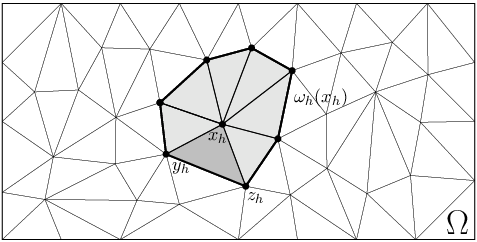
For an interior nodal point $x_{h}\in\Omega_{h}$ we consider the simplicial neighborhood $\omega_{h}(x_{h})$ , that is, the interior of the union of all simplices in $\Sigma_{h}$ that have $x_{h}$ as a vertex (see Figure 1).

Refer to caption — Figure 1. The neighborhood $\omega_{h}(x_{h})$ of $x_{h}\in\Omega_{h}$ , that is, the collection of all simplices (like the one shaded in dark) that have $x_{h}$ as a vertex.

The Idea.

The finite-element discretization which we propose is motivated by the idea of local solutions:

At $x_{h}\in\Omega_{h}$ the finite-element solution $u_{h}\in V_{h}$ takes the value $u_{h}^{*}(x_{h})$ of the exact viscosity solution $u_{h}^{*}\in C^{0,1}(\overline{\omega_{h}(x_{h})})$ that solves a simplified Hamilton-Jacobi equation on $\omega_{h}(x_{h})$ subject to the boundary conditions $u_{h}^{*}|_{\partial\omega_{h}(x_{h})}=u_{h}|_{\partial\omega_{h}(x_{h})}$ .

A good candidate for such a simplification of the Hamilton-Jacobi equation (4) is obtained by freezing locally the dependence of $H$ on its first variable. This way $u^{*}_{h}\in C^{0,1}(\overline{\omega_{h}(x_{h})})$ is obtained as the viscosity solution of the local Dirichlet problem

H(x_{h},Du^{*}_{h}(x))=0\;\;\text{on $\omega(x_{h})$},\qquad u_{h}^{*}|_{\partial\omega_{h}(x_{h})}=u_{h}|_{\partial\omega_{h}(x_{h})}.

(10)

This simplification is particularly suitable, because for $[y,z]\subset\overline{\omega_{h}(x_{h})}$ the optical distance $\delta_{x_{h}}(y,z)$ of the local equation (10) is, by Lemma 4,

\delta_{x_{h}}(y,z)=\rho(x_{h},y-z),

where $\rho(x_{h},\cdot)$ is the support function of the zero-level set of the convex function $H(x_{h},\cdot)$ as defined in (6). Theorem 1 tells us that if the local Dirichlet problem (10) is solvable, then the value $u_{h}^{*}(x_{h})$ is given by the Hopf–Lax formula

u_{h}^{*}(x_{h})=\min_{y\in\partial\omega_{h}(x_{h})}\Big(u_{h}(y)+\rho(x_{h},x_{h}-y)\Big),

that is, by a simple local variational principle. We note that, under the assumptions (H1)–(H4), the Hopf–Lax formula is well-defined independently of the compatibility of the boundary data of the local Dirichlet problem (10). Anyway, we base the finite-element discretization on this formula and the convergence will be proved later without the interpretation of $u_{h}^{*}$ as a local solution.

The Discretization

We define a function $\Lambda_{h}:V_{h}\to V_{h}$ , called the Hopf–Lax update function, by

(\Lambda_{h}u_{h})(x_{h})=\begin{cases}\displaystyle\min_{y\in\partial\omega_{h}(x_{h})}\Big(u_{h}(y)+\rho(x_{h},x_{h}-y)\Big),\qquad&x_{h}\in\Omega_{h},\\[8.53581pt] u_{h}(x_{h}),&x_{h}\in\partial\Omega_{h}.\end{cases}

The finite-element solution $u_{h}\in V_{h}$ that discretizes the Dirichlet problem (1) is now implicitly defined by the fixed-point equation

u_{h}=\Lambda_{h}u_{h},\qquad u_{h}|_{\partial\Omega_{h}}=g|_{\partial\Omega_{h}}.

(11)

As in the continuous case, we call $u_{h}\in V_{h}$ a finite-element subsolution (supersolution) if $u_{h}\leqslant\Lambda_{h}u_{h}$ ( $u_{h}\geqslant\Lambda_{h}u_{h}$ ).

We remark that the evaluation of $(\Lambda_{h}u_{h})(x_{h})$ at an interior nodal point $x_{h}\in\Omega_{h}$ can be calculated by a finite collection of $(d-1)$ -dimensional convex optimization problems. This follows from the representation (see Figure 1)

(\Lambda_{h}u_{h})(x_{h})=\min_{\sigma\in\Sigma_{h}:x_{h}\in\sigma}\min\Big\{u_{h}(y)+\rho(x_{h},x_{h}-y):\\ y\in\text{the ($d-1$)-dimensional face of $\sigma$ opposite to $x_{h}$}\Big\}

(12)

and the observation that $u_{h}$ is affine, and hence $u_{h}+\rho(x_{h},x_{h}-\cdot)$ convex, on $\sigma$ . In §7 we will study an important class of examples for which these $(d-1)$ -dimensional convex optimization problems allow for a particularly simple solution. In general, however, one would have to use suitable iterative numerical methods to solve them.

Remark.

For the particular Hamilton–Jacobi–Bellman equation (8) the finite-element discretization (11) is equivalent to various grid-based methods that are obtained from linear interpolation of the grid values and a direct local application of Bellman’s dynamic programming principle. See, e.g., [Tsi95, Eq. (2.3)] and [SV03, Eq. (25)] as well as the references given therein.

5. Existence and Uniqueness of the Finite-Element Solution

The existence of a finite-element solution as implicitly defined by (11) is based on two simple properties of the Hopf–Lax update function $\Lambda_{h}$ .

Lemma 5.

Assume (H1)–(H4). Let $u_{h},v_{h}\in V_{h}$ .

(1)

$\Lambda_{h}$ is monotone, that is, $u_{h}\leqslant v_{h}$ implies $\Lambda_{h}u_{h}\leqslant\Lambda_{h}v_{h}$ .
(2)

$\Lambda_{h}$ is nonexpanding, that is, $\left\|\Lambda_{h}u_{h}-\Lambda_{h}v_{h}\right\|_{\infty}\leqslant\left\|u_{h}-v_{h}\right\|_{\infty}$ .

Proof.

The first property is an immediate consequence of the definition of $\Lambda_{h}$ . To prove the second, let the maximum be attained at a nodal point $x_{h}\in\overline{\Omega}_{h}$ , without loss of generality $\left\|\Lambda_{h}u_{h}-\Lambda_{h}v_{h}\right\|_{\infty}=(\Lambda_{h}u_{h})(x_{h})-(\Lambda_{h}v_{h})(x_{h})$ . If $x_{h}\in\partial\Omega_{h}$ there is nothing to show; so we can assume $x_{h}\in\Omega_{h}$ . Let $y_{*}\in\partial\omega_{h}(x_{h})$ be such that

(\Lambda_{h}v_{h})(x_{h})=v_{h}(y_{*})+\rho(x_{h},x_{h}-y_{*}).

(13)

Hence

(\Lambda_{h}u_{h})(x_{h})-(\Lambda_{h}v_{h})(x_{h})\\[2.84526pt] \leqslant\Big(u_{h}(y_{*})+\rho(x_{h},x_{h}-y_{*})\Big)-\Big(v_{h}(y_{*})+\rho(x_{h},x_{h}-y_{*})\Big)\leqslant\left\|u_{h}-v_{h}\right\|_{\infty},

which proves the assertion. ∎

Theorem 6.

Assume (H1)–(H4) and $g:\partial\Omega\to\mathbb{R}$ . Then the finite-element discretization (11) has a solution $u_{h}\in V_{h}$ . If $u^{0}_{h}\in V_{h}$ is such that $u^{0}_{h}|_{\partial\Omega_{h}}=g|_{\partial\Omega_{h}}$ and $\Lambda_{h}u_{h}^{0}\geqslant u_{h}^{0}$ , then the fixed point iteration

u_{h}^{n+1}=\Lambda_{h}u^{n}_{h},\qquad n=0,1,2,\ldots,

converges monotonously to a solution of (11).

Proof.

An initial iterate $u^{0}_{h}\in V_{h}$ with $\Lambda_{h}u_{h}^{0}\geqslant u_{h}^{0}$ is given by

u^{0}_{h}|_{\partial\Omega_{h}}=g|_{\partial\Omega_{h}},\qquad u_{h}|_{\Omega_{h}}=\min_{x\in\partial\Omega_{h}}g(x).

Inductively the monotonicity of $\Lambda_{h}$ implies $u^{n+1}_{h}=\Lambda_{h}u^{n}_{h}\geqslant u_{h}^{n}$ . Hence, the monotone convergence of the sequence follows if we establish a uniform bound on the iterates. Since such a bound is trivial for the boundary we consider for a given $x_{h}\in\Omega_{h}$ a shortest path $x_{h}=x_{h}^{0},\ldots,x_{h}^{m}$ of nodal points that connects $x_{h}$ along edges of the triangulation with the boundary: $x_{h}^{m}\in\partial\Omega_{h}$ . There is a bound $L$ on the length of such a path which depends on the triangulation but not on $x_{h}$ . With $\rho^{*}$ as defined in Lemma 3 we get

u_{h}^{n}(x_{h})\leqslant\max_{y\in\partial\Omega_{h}}g(y)+\sum_{i=0}^{m-1}\rho(x_{h}^{i},x_{h}^{i}-x_{h}^{i+1})\leqslant\max_{y\in\partial\Omega_{h}}g(y)+\rho^{*}L.

(14)

Thus, $u_{h}^{n}\to u_{h}\in V_{h}$ for some $u_{h}\in V_{h}$ , which by continuity must be a fixed point of $\Lambda_{h}$ . ∎

Like in the continuous case, uniqueness of the finite-element solution requires the sharper condition (H4^′) and is a simple corollary of the following discrete comparison principle. Thus, the finite-element discretization is a monotone scheme.

Theorem 7.

Assume (H1)–(H3) and (H4^′). Let $u_{h},v_{h}\in V_{h}$ be finite-element sub- and supersolutions, respectively. If $u_{h}\leqslant v_{h}$ on $\partial\Omega_{h}$ then $u_{h}\leqslant v_{h}$ on $\overline{\Omega}$ .

Proof.

Let be $\Delta_{h}=u_{h}-v_{h}\in V_{h}$ . Note that the maximum of $\Delta_{h}$ will be attained in a nodal point. We will show that the existence of $x_{h}\in\Omega_{h}$ with $\Delta_{h}(x_{h})=\max_{x\in\overline{\Omega}}\Delta_{h}(x)=\delta>0$ yields a contradiction. To this end we choose such a maximizing $x_{h}$ with minimal value of $v_{h}(x_{h})$ . With $y_{*}\in\partial\omega_{h}(x_{h})$ as in (13) we get

\delta=u_{h}(x_{h})-v_{h}(x_{h})\leqslant(\Lambda_{h}u_{h})(x_{h})-(\Lambda_{h}v_{h})(x_{h})\leqslant u_{h}(y_{*})-v_{h}(y_{*}).

On the boundary of the face that contains $y_{*}$ in its relative interior there is, by the maximality of $\delta$ , a point $x_{h}^{*}\in\Omega_{h}$ such that $\Delta_{h}(x_{h}^{*})=\delta$ and $v_{h}(x_{h}^{*})\leqslant v_{h}(y_{*})$ . By Lemma 3 we have $\rho(x_{h},x_{h}-y_{*})>0$ and obtain

v_{h}(x_{h}^{*})\leqslant v_{h}(y_{*})=(\Lambda_{h}v_{h})(x_{h})-\rho(x_{h},x_{h}-y_{*})<(\Lambda_{h}v_{h})(x_{h})\leqslant v_{h}(x_{h})

in contradiction to the minimality of $v_{h}(x_{h})$ . ∎

In the discrete case, up to now, we did not impose a compatibility condition on the boundary data such as (H5). This will change in the discussion of a third important property of the finite-element solutions needed for convergence, that is, uniform Lipschitz continuity. Based on the constant $\rho_{*}\geqslant 0$ of Lemma 4 and the regularity constant $\theta\geqslant 1$ of the family of triangulation we consider the condition

(H5^′)

$g(x)-g(y)\leqslant\dfrac{\rho_{*}}{\theta}\left\|x-y\right\|$ for all $x,y\in\partial\Omega$ .

By Lemma 4 this condition is actually stronger than (H5). Note that the homogeneous Dirichlet condition $g=0$ always satisfies (H5^′).

Theorem 8.

Assume (H1)–(H3), (H4^′) and (H5^′). The unique finite-element solution $u_{h}\in V_{h}$ of (11) satisfies the uniform Lipschitz condition

|u_{h}(x)-u_{h}(y)|\leqslant c_{\Omega}\,\theta d\cdot\rho^{*}\cdot\left\|x-y\right\|,\qquad x,y\in\overline{\Omega},

and the uniform bound

\|u_{h}\|_{\infty}\leqslant\max_{x\in\partial\Omega}|g(x)|+c_{\Omega}\,\theta d\cdot\rho^{*}\cdot\operatorname{diam}(\Omega).

Here, $\theta$ denotes the regularity constant of the family of triangulations, $\rho^{*}$ is the constant defined in Lemma 3 and $c_{\Omega}>0$ is a constant depending only on $\Omega$ . If $\Omega$ is convex, we can choose $c_{\Omega}=1$ .

Proof.

The uniform bound on $\left\|u_{h}\right\|_{\infty}$ is a simple consequence of the Lipschitz condition. The proof of the Lipschitz condition proceeds in three steps, imposing less and less restrictions on the possible choices of $x,y\in\overline{\Omega}$ .

Step 1.

For neighboring nodal points $x_{h},y_{h}\in\overline{\Omega}_{h}$ we prove

|u_{h}(x_{h})-u_{h}(y_{h})|\leqslant\rho^{*}\cdot\left\|x_{h}-y_{h}\right\|.

Since $\rho^{*}\geqslant\rho_{*}\geqslant\rho_{*}/\theta$ this is, by (H5^′), obviously true for $x_{h},y_{h}\in\partial\Omega_{h}$ . If $x_{h}\in\Omega_{h}$ we have $y_{h}\in\partial\omega_{h}(x_{h})$ and hence

u_{h}(x_{h})=(\Lambda_{h}u_{h})(x_{h})\leqslant u_{h}(y_{h})+\rho(x_{h},x_{h}-y_{h})\leqslant u_{h}(y_{h})+\rho^{*}\left\|x_{h}-y_{h}\right\|.

If $y_{h}\in\Omega_{h}$ we can change the roles of $x_{h}$ and $y_{h}$ and the Lipschitz bound follows.

Assume on the other hand that $y_{h}\in\partial\Omega_{h}$ . There is a minimizing $y_{*}\in\partial\omega_{h}(x_{h})$ such that

u_{h}(x_{h})=(\Lambda_{h}u_{h})(x_{h})=u_{h}(y_{*})+\rho(x_{h},x_{h}-y_{*})>u_{h}(y_{*}),

where the last inequality follows from Lemma 3. The boundary of the face that contains $y_{*}$ in its relative interior has a point $x_{h}^{1}\in\overline{\Omega}_{h}$ with $u_{h}(x_{h}^{1})\leqslant u_{h}(y_{*})<u_{h}(x_{h})$ . By the definition of $\rho_{*}$ and $\theta$ we obtain

\rho(x_{h},x_{h}-y_{*})\geqslant\rho_{*}\|x_{h}-y_{*}\|\geqslant\frac{\rho_{*}}{\theta}\|x_{h}-x_{h}^{1}\|.

Continuing this construction we obtain a sequence $x_{h}=x_{h}^{0},x_{h}^{1},\ldots,x_{h}^{m}$ of nodal points with strictly decreasing $u_{h}$ -values that necessarily reaches the boundary at some index $m$ : $x_{h}^{m}\in\partial\Omega_{h}$ . Thus, by construction and (H5^′),

u_{h}(x_{h})\geqslant g(x_{h}^{m})+\frac{\rho_{*}}{\theta}\sum_{i=0}^{m-1}\|x_{h}^{i}-x_{h}^{i+1}\|\\[5.69054pt] \geqslant g(y_{h})+\frac{\rho_{*}}{\theta}\left(\sum_{i=0}^{m-1}\|x_{h}^{i}-x_{h}^{i+1}\|-\|x_{h}^{m}-y_{h}\|\right)\\[5.69054pt] \geqslant u_{h}(y_{h})-\frac{\rho_{*}}{\theta}\left\|x_{h}-y_{h}\right\|\geqslant u_{h}(y_{h})-\rho^{*}\left\|x_{h}-y_{h}\right\|,

which concludes the proof of Step 1.

Step 2.

Let $\sigma\in\Sigma_{h}$ be a simplex of the triangulation. For $x,y\in\sigma$ we prove that

|u_{h}(x)-u_{h}(y)|\leqslant\theta d\cdot\rho^{*}\cdot\left\|x-y\right\|.

By an affine transformation $\hat{x}\mapsto B\hat{x}+b$ we map the standard $d$ -dimensional simplex

\hat{\sigma}=\{\hat{x}\in\mathbb{R}^{d}_{\geqslant 0}:\hat{x}_{1}+\ldots+\hat{x}_{d}\leqslant 1\}

onto $\sigma$ . The pullback of $u_{h}|_{\sigma}$ under the transformation will be denoted $\hat{u}$ . By Step 1 we can estimate the length of the (constant) gradient of $u_{h}|_{\sigma}$ by

\|Du_{h}|_{\sigma}\|\leqslant\|B^{-1}\|\,\|D\hat{u}\|\leqslant\|B^{-1}\|\sqrt{d}\,\rho^{*}\cdot h_{1}(\sigma).

Now, $\|B^{-1}\|$ is the largest ratio of the length of a segment in $\hat{\sigma}$ to the length of its image in $\sigma$ . Without loss of generality such a segment can be assumed to join a vertex with the opposite boundary face. Thus $\|B^{-1}\|\leqslant\sqrt{d}/h_{0}(\sigma)$ and, by the shape-regularity assumption, that is, $h_{1}(\sigma)/h_{0}(\sigma)\leqslant\theta$ , we get

\|Du_{h}|_{\sigma}\|\leqslant\theta d\cdot\rho^{*}

and hence the assertion of Step 2.

Step 3.

For $x,y\in\overline{\Omega}$ there is a Lipschitz path $\gamma\in C^{0,1}([0,1],\overline{\Omega})$ joining $x$ and $y$ such that (see [Alt99, p. 304])

\left\|\gamma^{\prime}\right\|_{\infty}\leqslant c_{\Omega}\|x-y\|.

For convex $\Omega$ the path $\gamma$ can be chosen as the segment joining $x$ and $y$ , which yields $c_{\Omega}=1$ . Now, let $0=t_{0}<t_{1}<\ldots<t_{m}=1$ be a subdivision of $[0,1]$ such that $\gamma(t_{i-1})$ and $\gamma(t_{i})$ are elements of a common simplex. By Step 2 we obtain

|u_{h}(x)-u_{h}(y)|\leqslant\sum_{i=0}^{m-1}|u_{h}(\gamma(t_{i}))-u_{h}(\gamma(t_{i+1}))|\leqslant\theta d\cdot\rho^{*}\sum_{i=0}^{m-1}\|\gamma(t_{i})-\gamma(t_{i+1})\|\\[5.69054pt] \leqslant c_{\Omega}\,\theta d\cdot\rho^{*}\cdot\|x-y\|\sum_{i=0}^{m-1}|t_{i}-t_{i+1}|=c_{\Omega}\,\theta d\cdot\rho^{*}\cdot\|x-y\|,

which concludes the proof of the asserted Lipschitz bound. ∎

6. Convergence of the Finite-Element Discretization

The argument will be simplified if we consider a modified Hamiltonian $\tilde{H}$ for which the corresponding Hamilton-Jacobi equation possesses the same viscosity solutions as the original one.

Lemma 9.

Assume (H1)–(H4). Let $x\in\bar{\Omega}$ and $p\in\mathbb{R}^{d}$ . For the modified Hamiltonian

\tilde{H}(x,p)=\max_{\|q\|=1}\left(\langle p,q\rangle-\rho(x,q)\right)

we get that $\tilde{H}(x,p)\leqslant 0$ ( $\tilde{H}(x,p)\geqslant 0$ ) implies $H(x,p)\leqslant 0$ ( $H(x,p)\geqslant 0$ ).

Proof.

First assume $H(x,p)>0$ . There is a hyperplane that separates $p$ strongly from the compact and convex level set $\{\tilde{p}:H(x,\tilde{p})\leqslant 0\}$ (see [Roc70, Cor. 11.4.2]). That is, there is a vector $q\in\mathbb{R}^{d}$ , $\left\|q\right\|=1$ , with $\rho(x,q)<\langle p,q\rangle$ . Hence

\tilde{H}(x,p)\geqslant\langle p,q\rangle-\rho(x,q)>0.

Now assume $H(x,p)<0$ . There is $\epsilon>0$ such that $H(x,p+\delta p)<0$ for $\left\|\delta p\right\|\leqslant\epsilon$ . Hence

\langle p,q\rangle-\rho(x,q)\leqslant\langle p,q\rangle-\max_{\left\|\delta p\right\|\leqslant\epsilon}\langle p+\delta p,q\rangle=-\epsilon\left\|q\right\|,

Taking the supremum over all $q$ with $\left\|q\right\|=1$ yields $\tilde{H}(x,p)\leqslant-\epsilon<0$ . ∎

In particular, each viscosity subsolution (supersolution) of the thus modified Hamilton–Jacobi equation $\tilde{H}(x,Du(x))=0$ , $x\in\Omega$ , is also a viscosity subsolution (supersolution) of the original one $H(x,Du(x))=0$ , $x\in\Omega$ .²² 2 Under the additional assumption (H4^′) the same holds true, since then $\rho(x,q)>0$ for $x\in\Omega$ , if we consider the modified Hamilton–Jacobi equation with the Hamiltonian $\tilde{H}(x,p)=\max_{\|q\|=1}\frac{\left\langle p,q\right\rangle}{\rho(x,q)}-1.$ Hence, we see that the example at the end of §2 in fact covers the general case.

Loosely speaking, in the framework of viscosity solutions the notion of consistency of a discretization means that a smooth function is already a subsolution (supersolution) of the differential equation if it is a subsolution (supersolution) of the discrete scheme. The precise statement is given in the next theorem.

Theorem 10.

Assume (H1)–(H3) and (H4^′). Let $v\in C^{\infty}_{0}(\Omega)$ , $x\in\Omega$ , and $x_{h}\in\Omega_{h}$ be a sequence of nodal points that converges to $x$ as $h\to 0$ . Then

	$\displaystyle v(x_{h})\leqslant(\Lambda_{h}I_{h}v)(x_{h})\;\;\text{for all $h$}$	$\displaystyle\quad\Rightarrow\quad H(x,Dv(x))\leqslant 0,$
	$\displaystyle v(x_{h})\geqslant(\Lambda_{h}I_{h}v)(x_{h})\;\;\text{for all $h$}$	$\displaystyle\quad\Rightarrow\quad H(x,Dv(x))\geqslant 0,$

where $I_{h}:C(\overline{\Omega})\to V_{h}$ denotes the nodal interpolation operator.

Proof.

Since $v$ is smooth we can approximate the directional derivatives of $v$ in $x_{h}$ by first order differences as follows

\frac{v_{h}(x_{h})-(I_{h}v)(y)}{\|x_{h}-y\|}=\left\langle Dv(x_{h}),\frac{x_{h}-y}{\left\|x_{h}-y\right\|}\right\rangle+O(h),\qquad y\in\partial\omega_{h}(x_{h}).

(15)

Now, let $v(x_{h})\leqslant(\Lambda_{h}I_{h}v)(x_{h})$ for all $h$ of the sequence, that is,

v(x_{h})-(I_{h}v)(y)-\rho(x_{h},x_{h}-y)\leqslant 0,\qquad y\in\partial\omega_{h}(x_{h}).

After division by $\|x_{h}-y\|$ we get, by (15), a constant $c>0$ such that

\langle Dv(x_{h}),q\rangle-\rho(x_{h},q)\leqslant ch,\qquad\|q\|=1.

If we pass to the limit $h\to 0$ (note the continuity of $\rho$ at $x\in\Omega$ as stated in Lemma 3) and take thereafter the maximum over all $\|q\|=1$ , we obtain

\tilde{H}(x,Dv(x))=\max_{\|q\|=1}(\langle Dv(x),q\rangle-\rho(x,q))\leqslant 0.

From Lemma 9 we infer the assertion $H(x,Dv(x))\leqslant 0$ .

On the other hand, let $v(x_{h})\geqslant(\Lambda_{h}I_{h}v)(x_{h})$ for all $h$ of the sequence, that is,

v(x_{h})-(I_{h}v)(y_{h})-\rho(x_{h},x_{h}-y_{h})\geqslant 0

for some $y_{h}\in\partial\omega_{h}(x_{h})$ . After devision by $\|x_{h}-y_{h}\|$ we get, by (15), a constant $c>0$ such that

\langle Dv(x_{h}),q_{h}\rangle-\rho(x_{h},q_{h})\geqslant-ch,\qquad q_{h}=(x_{h}-y_{h})/\|x_{h}-y_{h}\|.

By compactness, we can assume that $q_{h}\to q_{*}$ with $\|q_{*}\|=1$ . Passing to the limit $h\to 0$ we thus obtain

\tilde{H}(x,Dv(x))\geqslant\langle Dv(x),q_{*}\rangle-\rho(x,q_{*})\geqslant 0,

from which we infer the assertion $H(x,Dv(x))\geqslant 0$ by Lemma 9. ∎

Now we have all the tools in hand to prove the convergence of the finite-element discretization.

Theorem 11.

Assume (H1)–(H3), (H4^′), and (H5^′). Then, as $h\to 0$ , the sequence of unique finite-element solutions $u_{h}\in V_{h}$ defined by

u_{h}=\Lambda_{h}u_{h},\qquad u_{h}|_{\partial\Omega_{h}}=g|_{\partial\Omega_{h}},

converges uniformly to the unique viscosity solution $u$ of the Dirichlet problem

H(x,Du(x))=0,\qquad u|_{\partial\Omega}=g.

Proof.

Theorems 6 and 7 show the existence and uniqueness of the finite-element solutions $u_{h}\in V_{h}$ . Theorem 8 shows that $u_{h}\in V_{h}$ is a uniform bounded sequence of uniform Lipschitz continuous functions. By the theorem of Arzelà–Ascoli there is a subsequence $(u_{h^{\prime}})$ that converges uniformly to a function $u\in C^{0,1}(\overline{\Omega})$ . Because of (H5^′) and $u_{h}|_{\partial\Omega_{h}}=g|_{\partial\Omega_{h}}$ , this limit satisfies the boundary condition $u|_{\partial\Omega}=g$ .

To show that $u$ is a viscosity subsolution of $H(x,Du(x))=0$ let $v\in C^{\infty}_{0}(\Omega)$ and $x_{0}\in\Omega$ such that $u-v$ attains a local maximum in $x_{0}$ . By adding a quadratic parabola to $v$ if necessary, we may assume that it is in fact a strict local maximum (see [Eva98, p. 542]). Extracting a further subsequence of $h^{\prime}$ if necessary, there is, by uniform convergence and the monotonicity of the nodal interpolation operator $I_{h}:C(\overline{\Omega})\to V_{h}$ , a sequence of nodal points $x_{h^{\prime}}\in\Omega_{h^{\prime}}$ such that $x_{h^{\prime}}\to x_{0}$ and (see the argument given in [Eva98, p. 541])

(u_{h^{\prime}}-v)(x_{h^{\prime}})\geqslant(u_{h^{\prime}}-I_{h^{\prime}}v)(y),\qquad y\in\partial\omega_{h^{\prime}}(x_{h^{\prime}}).

Now let $y_{*}\in\partial\omega_{h^{\prime}}(x_{h^{\prime}})$ be a minimizing argument such that

(\Lambda_{h^{\prime}}I_{h^{\prime}}v)(x_{h^{\prime}})=(I_{h^{\prime}}v)(y_{*})+\rho(x_{h^{\prime}},x_{h^{\prime}}-y_{*}).

Then it holds that

(u_{h^{\prime}}-v)(x_{h^{\prime}})\geqslant u_{h^{\prime}}(y_{*})+\rho(x_{h^{\prime}},x_{h^{\prime}}-y_{*})-(I_{h^{\prime}}v)(y_{*})-\rho(x_{h^{\prime}},x_{h^{\prime}}-y_{*})\\ \geqslant(\Lambda_{h^{\prime}}u_{h^{\prime}}-\Lambda_{h^{\prime}}I_{h^{\prime}}v)(x_{h^{\prime}})=(u_{h^{\prime}}-\Lambda_{h^{\prime}}I_{h^{\prime}}v_{h^{\prime}})(x_{h^{\prime}})

and thus

v(x_{h^{\prime}})\leqslant(\Lambda_{h^{\prime}}I_{h^{\prime}}v)(x_{h^{\prime}}).

The consistency of the discretization, stated in Theorem 10, yields that

H(x_{0},Dv(x_{0}))\leqslant 0,

which concludes the proof that $u$ is a viscosity subsolution.

In the same way we prove that $u$ is a viscosity supersolution of $H(x,Du(x))=0$ . Therefore, $u$ is a viscosity solution, which, by the comparison principle (Theorem 2), is actually unique. Hence, there is exactly one limit point of the sequence $u_{h}$ , which thus has to converge uniformly to the just established viscosity solution $u$ . ∎

Remark

Note that the only use that we have made so far of the existence Theorem 1 was to motivate the local variational principle for the finite-element discretization. In fact, our proof of the convergence result shows the existence of a viscosity solution en route — under the somewhat more restrictive compatibility conditions (H4^′) and (H5^′), however.

7. The Hopf–Lax Update for Generalized Eikonal Equations in 2D

Let $\Omega\subset\mathbb{R}^{2}$ be a polygonal Lipschitz domain and $M:\overline{\Omega}\to\mathbb{R}^{2\times 2}$ be a continuous mapping into the symmetric positive definite $2\times 2$ -matrices. We denote the corresponding inner product by $\langle p,q\rangle_{M(x)}=\langle M(x)p,q\rangle$ , its subordinate norm by $\|p\|_{M(x)}=\langle p,p\rangle_{M(x)}^{1/2}$ .

Now, we consider the Dirichlet problem for the generalized eikonal equation,

\|Du\|_{M(x)}=1\;\;\text{in $\Omega$},\qquad u|_{\partial\Omega}=g.

Its Hamiltonian $H(x,p)=\|p\|_{M(x)}-1$ satisfies the assumptions (H1)–(H3) and (H4^′). The support function of the zero-level set is simply given by the norm that is dual to $\|\cdot\|_{M(x)}$ , namely,

\rho(x,q)=\max_{H(x,p)=0}\langle p,q\rangle=\max_{\|p\|_{M(x)}=1}\langle p,q\rangle=\|q\|_{M(x)^{-1}}.

The Hopf–Lax update function becomes

(\Lambda_{h}u_{h})(x_{h})=\min_{y\in\partial\omega_{h}(x_{h})}\Big(u_{h}(y)+\|x_{h}-y\|_{M(x_{h})^{-1}}\Big),\qquad x_{h}\in\Omega_{h},\;u_{h}\in V_{h}.

There is a simple procedure to evaluate $(\Lambda_{h}u_{h})(x_{h})$ at $x_{h}\in\Omega_{h}$ . To this end let $\sigma_{1},\ldots,\sigma_{m}\in\Sigma_{h}$ be the triangles that have $x_{h}$ as a vertex and $J_{i}$ the (closed) edge of $\sigma_{i}$ opposite to $x_{h}$ . Then, as in (12),

(\Lambda_{h}u_{h})(x_{h})=\min_{1\leqslant i\leqslant m}u_{i}\qquad\text{with}\qquad u_{i}=\min_{y\in J_{i}}\Big(u_{h}(y)+\|x_{h}-y\|_{M(x_{h})^{-1}}\Big).

Let us take one of the triangles, $\sigma_{i}$ , (see Figure 1) and call its vertices $x_{h}$ , $y_{h}$ , $z_{h}$ , hence $J_{i}=[y_{h},z_{h}]$ . In the case of the classic eikonal equation, that is, $M(x)\equiv I$ , the update $u_{i}$ can be determined from an elementary geometric argument.

Lemma 12.

Let $\sigma\in\Sigma_{h}$ be the triangle with the vertices $x_{h}$ , $y_{h}$ , $z_{h}$ and $u_{h}\in V_{h}$ . Denote the angles at $y_{h}$ , $z_{h}$ by $\alpha$ , $\beta$ , respectively. Defining

\Delta=\frac{u_{h}(z_{h})-u_{h}(y_{h})}{\|z_{h}-y_{h}\|}

and $\cos(\delta)=\Delta$ if $|\Delta|\leqslant 1$ , we obtain

u_{i}=\min_{y\in[y_{h},z_{h}]}\Big(u_{h}(y)+\|x_{h}-y\|\Big)=u_{h}(y_{h})+\min_{y\in[y_{h},z_{h}]}\Big(\Delta\cdot\|y-y_{h}\|+\|x_{h}-y\|\Big)\\[5.69054pt] =\begin{cases}u_{h}(y_{h})+\|x_{h}-y_{h}\|,&\qquad\cos(\alpha)\leqslant\Delta,\\[2.84526pt] u_{h}(y_{h})+\cos(\delta-\alpha)\cdot\|x_{h}-y_{h}\|,&\qquad\alpha\leqslant\delta\leqslant\pi-\beta,\\[2.84526pt] u_{h}(z_{h})+\|x_{h}-z_{h}\|,&\qquad\Delta\leqslant\cos(\pi-\beta).\end{cases}

Proof.

For $|\Delta|\geqslant 1$ the assertion follows from a direct application of the triangle inequality; e.g., for $\Delta\geqslant 1$ ,

\Delta\cdot\|y-y_{h}\|+\|x_{h}-y\|\geqslant\|y-y_{h}\|+\|x_{h}-y\|\geqslant\|x_{h}-y_{h}\|.

Now, let $|\Delta|<1$ so that $\cos(\delta)=\Delta$ defines a $\delta\in(0,\pi)$ . A look at Figure 2 shows that

\cos(\delta)\cdot\|y-y_{h}\|+\|x_{h}-y\|

(16)

attains its minimum at the unique intersection $y_{*}$ of two straight lines: the first line running through $y_{h}$ and $z_{h}$ , the second line running through $x_{h}$ perpendicular to $l_{\delta}$ . Here, $l_{\delta}$ is the straight line that encloses at $y_{h}$ with $[y_{h},z_{h}]$ the angle $\pi/2-\delta$ . We observe that the value of the minimum is simply $\cos(\delta-\alpha)\cdot\|x_{h}-y_{h}\|$ . A further look at Figure 2 teaches that $y_{*}\in[y_{h},z_{h}]$ if and only if

0\leqslant\delta-\alpha\leqslant\gamma=\pi-\alpha-\beta,\qquad\text{that is,}\qquad\alpha\leqslant\delta\leqslant\pi-\beta.

If $\delta<\alpha$ , or equivalently $\Delta>\cos(\alpha)$ , $y_{*}$ is to the left of $y_{h}$ and the minimum of (16) in $[y_{h},z_{h}]$ is attained at $y_{h}$ . On the other hand, if $\delta>\pi-\beta$ , or equivalently $\Delta<\cos(\pi-\beta)$ , $y_{*}$ is to the right of $z_{h}$ and the minimum of (16) in $[y_{h},z_{h}]$ is attained at $z_{h}$ . ∎

For the general case we simple apply the triangular update formula of Lemma 12 to the image of the triangle $\sigma_{i}$ under the linear transformation $M(x_{h})^{-1/2}$ . This way we immediately obtain the following update procedure, writing $\langle p,q\rangle_{x}=\langle p,q\rangle_{M(x)^{-1}}$ , $\|p\|_{x}=\|p\|_{M(x)^{-1}}$ , $c_{\alpha}=\cos(\alpha)$ , and $c_{\beta}=\cos(\beta)$ for short (note that we used the addition formula to spell out $\cos(\alpha-\delta)$ for implementation purposes):

		$\displaystyle\Delta=\dfrac{u_{h}(z_{h})-u_{h}(y_{h})}{\\|z_{h}-y_{h}\\|_{x_{h}}};$
		$\displaystyle c_{\alpha}=\dfrac{\langle x_{h}-y_{h},z_{h}-y_{h}\rangle_{x_{h}}}{\\|x_{h}-y_{h}\\|_{x_{h}}\cdot\\|z_{h}-y_{h}\\|_{x_{h}}};\quad c_{\beta}=\dfrac{\langle x_{h}-z_{h},y_{h}-z_{h}\rangle_{x_{h}}}{\\|x_{h}-z_{h}\\|_{x_{h}}\cdot\\|y_{h}-z_{h}\\|_{x_{h}}};$
		$\displaystyle\texttt{if}\;\;c_{\alpha}\leqslant\Delta$
		$\displaystyle\qquad u_{i}=u_{h}(y_{h})+\\|x_{h}-y_{h}\\|_{x_{h}};$
		$\displaystyle\texttt{else if}\;\;\Delta\leqslant-c_{\beta}$
		$\displaystyle\qquad u_{i}=u_{h}(z_{h})+\\|x_{h}-z_{h}\\|_{x_{h}};$
		else
		$\displaystyle\qquad u_{i}=u_{h}(y_{h})+\left(c_{\alpha}\Delta+\sqrt{(1-c_{\alpha}^{2})(1-\Delta^{2})}\right)\\|x_{h}-y_{h}\\|_{x_{h}};$

Remark

With different ideas on a discretization, exactly the same update formula has been obtained for the (classic) eikonal equation by Kimmel and Sethian [KS98] (see also [Set99, §10.3.1]), who use for acute triangulations the methodology of [BS98] to construct upwind schemes on unstructured meshes, and, independently, by the geophysicist Fomel [Fom97], who locally uses Fermat’s principle of shortest travel times (which is closely related to our local use of the Hopf–Lax formula).

Sethian [Set99, §10.1] shows further that this update formula generalizes the upwind finite-difference scheme on structured grids given by Rouy and Tourin [RT92].

8. Solving the Discrete System

A Review of Methods.

Theorem 6 shows that the nonlinear discrete system (11) can be solved by the fixed-point iteration

u_{h}^{n+1}=\Lambda_{h}u_{h}^{n},\quad n=0,1,2,\ldots,

for a suitably chosen initial iterate $u^{0}_{h}$ . Such a fixed-point iteration uses the updated values at a nodal point $x_{j}$ only after all the updated values have been calculated. This corresponds to the classic Jacobi–iteration for linear systems of equations and lends itself to direct parallelization.

If we sequentially traverse the nodal points in a given order and modify the iteration to always use the most recently updated value, we obtain a nonlinear variant of the Gauss–Seidel iteration. Rouy and Tourin [RT92] used such a nonlinear Gauss-Seidel iteration to solve a finite difference discretization of the eikonal equation $\left\|Du(x)\right\|=n(x)$ on a structured mesh.

For both iterative methods the complexity will typically scale as $O(N^{1+1/d})$ , where $N$ denotes the number of nodal points and $d$ the space dimension. This is because the information about the solution, inherent initially to the boundary only, travels by next neighbor interaction at each run trough all nodal points. To spread that information to the whole computational domain about $O(N^{1/d})$ runs are necessary. However, even though this heuristic well explains the experimental observations, to our knowledge there is no rigorous proof of that in the literature.

In 1995 Sethian [Set96] and Tsitsiklis [Tsi95] have shown independently that for eikonal equations on structured meshes the nonlinear equation can be solved exactly in a single pass, that is, by traversing the grid once using local operations only. This fast marching method was later generalized to triangular meshes by Kimmel and Sethian [KS98]. It relies on the causality property, namely that on an acute triangulation the value $u_{h}(x_{h})$ depends only on the values in neighboring nodal points $y_{h}$ that are lower, $u_{h}(y_{h})\leqslant u_{h}(x_{h})$ . So the discrete solution can be computed starting from the neighborhood of the boundary moving further inwards the computational domain along increasing values of $u_{h}$ . However, on non-acute triangulations additional effort is necessary to deal with the loss of this causality property (see [KS98] for details). The complexity of this method is $O(N\log(N))$ where the logarithm comes from administering a priority queue of candidates for the next lowest value of $u_{h}$ , such as a heap data structure.

For the particular Hamilton–Jacobi–Bellman equation (8) a single pass algorithm generalizing the fast marching method, called the ordered upwind method (OUM), was introduced by Sethian and Vladimirsky [SV00] and is discussed in detail in [SV03]. This method is not a fast solver for a given discretization, but the discretization is specifically designed for the needs of the fast solver. Like the Hopf–Lax update the update formulas of the OUM are based on local variational principles (Bellman’s principle). However though, the OUM does not solve (11), since the update in $x_{h}$ is not necessarily computed from the neighborhood $\omega_{h}(x_{h})$ but from larger neighborhoods within the radius $h\cdot\nu$ . Here $\nu=F^{*}/F_{*}$ denotes the anisotropy coefficient of the Hamilton–Jacobi–Bellman equation (see (7)). This quantity $\nu$ affects not only the complexity of the OUM, which is $O(\nu^{d-1}N\log(N))$ , but also its accuracy.

Adaptive Nonlinear Gauss–Seidel Iteration.

In this paper we propose an adaptive version of the nonlinear Gauss-Seidel iteration, which is a modelled after a similar relaxation method [PR93] for the multilevel solution of elliptic boundary value problems. It turns out to be substantially faster than the standard Gauss-Seidel iteration, easy to implement and universal.

The adaptive Gauss-Seidel iteration differs from the standard one in two respects. First, like in the fast marching method, only those nodal points are updated that “have the information”, that is, are neighbors of recently updated points. Second, the order of updates is not fixed but varies as the iteration proceeds. Thus, a queue denoted by $\mathcal{Q}$ is administered to provide the ordering of updates. However, other than in the fast-marching method where using the causality property requires to keep control of the point with minimal function value, the queue is now simply given the structure of a FIFO (first in first out) stack: the nodal point staying longest in the queue is updated next.

The algorithm is passed a user-defined tolerance tol and it ends up with an approximate finite-element solution $u_{h}\in V_{h}$ such that

\left\|u_{h}-\Lambda_{h}u_{h}\right\|_{\infty}\leqslant\text{\rm tol}.

It is organized as follows:

(1)

(Initialization) Let $u_{h}|_{\partial\Omega_{h}}=g|_{\partial\Omega_{h}}$ , $u_{h}|_{\Omega_{h}}\equiv\infty$ .³³ 3 In fact any value larger than the bound (14) will do. However, taking $\infty$ makes the argument more elegant and can correctly be implemented in IEEE arithmetic. Let $\mathcal{Q}$ be the list of all points $x_{h}\in\Omega_{h}$ that are adjacent to some boundary point (in an arbitrary but fixed order).
(2)

(Iteration) Remove the first point $x_{h}$ from $\mathcal{Q}$ and compute the update value $u_{\rm new}=(\Lambda_{h}u_{h})(x_{h})$ .
(3)

If $|u_{\rm new}-u_{h}(x_{h})|>\text{\rm tol}$ then update $u_{h}(x_{h})=u_{\rm new}$ and append all not yet enqueued neighbors $y_{h}$ of $x_{h}$ to the queue $\mathcal{Q}$ .
(4)

If $\mathcal{Q}\not=\emptyset$ , goto (2).

To prove the convergence of this method, we denote the initial finite-element function of step 1 by $u_{h}^{0}$ . After the $n$ th update has been performed in step 3 the actual finite-element function will be denoted by $u_{h}^{n}$ .

Theorem 13.

The algorithm generates a sequence $u_{h}^{0},u_{h}^{1},\ldots$ , that is monotonously decreasing. It terminates after finitely many steps with an approximate finite element solution $u_{h}\in V_{h}$ , such that $\left\|u_{h}-\Lambda_{h}u_{h}\right\|\leqslant\text{\rm tol}$ .

Proof.

The initialization $u_{h}|_{\Omega_{h}}\equiv\infty$ ensures that every point $x_{h}$ is updated at least once, as the residual is $\infty$ when the first update value in $x_{h}$ is computed. After the first update, $u_{h}(x_{h})$ is assigned a finite value, since $x_{h}$ has a neighbor in $\partial\Omega_{h}$ or a neighbor, for which a finitely valued update has already been computed. By induction on $n$ we get that at each later update of a nodal point $x_{h}$ , all neighbors of $x_{h}$ that have been changed over the last update can only have been assigned a lower value of $u_{h}$ . ¿From the monotonicity of $\Lambda_{h}$ we thus get the first assertion.

Since an update in step (3) only affects the residual in the neighboring points, which are are immediately enqueued, it holds that

\{x_{h}\in\Omega_{h}\ :\ u_{h}^{n}(x_{h})<\infty\textrm{~and~}|\Lambda_{h}u_{h}^{n}-u_{h}^{n}|>\text{\rm tol}\}\ \subset\ \mathcal{Q}

for every $n\geqslant 0$ . So if the algorithm terminates with $\mathcal{Q}=\emptyset$ , the tolerance has been reached.

Otherwise, if the iteration does not terminate, then there is at least one nodal point $x_{h}^{*}$ that appears infinitely often as the first element of the queue $\mathcal{Q}$ and gets updated at steps $n_{j}\to\infty$ , $j\to\infty$ . Hence, there must be $|u_{h}^{n_{j}}(x_{h}^{*})-u_{h}^{n_{j}-1}(x_{h}^{*})|>\text{\rm tol}$ in contradiction to the convergence of $u_{h}^{n_{j}}(x_{h}^{*})$ as $j\to\infty$ which is implied by the monotonicity and the trivial lower bound $u_{h}^{n}\geqslant\min_{x\in\partial\Omega}g(x)$ . ∎

Though the run-time complexity of the adaptive Gauss–Seidel iteration behaves probably at worst as $O(N^{1+1/d})$ like in the standard Gauss-Seidel iteration, a lot of unnecessary updates are saved as we will see in the numerical experiments of the next section.

9. Numerical Experiments

For the two following examples the solutions were computed on unstructured meshes with $23^{2}$ , $45^{2}$ , $91^{2}$ , $181^{2}$ , and $725^{2}$ nodal points. A solution on a mesh with $1451^{2}$ points served to estimate the discretization error. The iterative methods were used with an absolute tolerance $\text{\rm tol}=10^{-8}$ .

The first example concerns the distance map on the torus given by the immersion

f(x_{1},x_{2})=\left(\cos(2\pi x_{1})(5+4\cos(2\pi x_{2})),\sin(2\pi x_{1})(5+4\cos(2\pi x_{2})),\sin(2\pi x_{2})\right).

Using the Gram matrix $G(x)=Df(x)^{T}Df(x)$ and $\rho^{2}(x,q)=\left\langle q,G(x)q\right\rangle$ the distance between the points $f(x)$ and $f(y)$ on the manifold is given by the function $\delta(x,y)$ as defined in (2). With the results of §7 and [Lio82, Thm. 5.3(iv)] we obtain that $u(x)=\delta(x,0)$ is the viscosity solution of the Dirichlet problem

\left\|Du\right\|_{G(x)^{-1}}=1\textrm{~on~}\Omega\setminus\{0\},\qquad u(0)=0,

where $\Omega=[-0.5,0.5]^{2}$ . The solution is shown to the left of Figure 3 as a contour plot.

To the right of Figure 3 we compare the accuracy and complexity of the adaptive Gauss-Seidel method with both the standard Gauss-Seidel iteration and the OUM.⁴⁴ 4 We have coded the OUM from [SV03] with a little completion that turned out to be necessary: Considered points have also to be updated, if they depend on an edge that drops out of the accepted front. If some point $x_{h}$ gets accepted this may happen to any edge opposite to $x_{h}$ in $\omega_{h}(x_{h})$ . Here, by complexity we mean the total number of updates calculated on a triangle by a formula such as the one at the end of §7. We observe that the adaptive Gauss–Seidel iteration is more than a factor of 10 faster than the standard Gauss–Seidel iteration but displays the same asymptotic rate of complexity. The OUM show, as theoretically expected, a better rate of complexity that, in this example, becomes significant even at larger tolerances.

The second example is taken from [SV01] and shows the effect of a moderately large anisotropy coefficient $\nu=19$ , which affects the complexity of the OUM. We consider a simple min-time optimal control problem governed by the dynamical system

y^{\prime}(t)=a(t)+b(y(t)),\qquad y(0)=x.

The controls $a(\cdot)$ are taken from $\mathcal{A}=\{a:[0,\infty)\rightarrow S^{1}\textrm{~measurable}\}$ and

b(y)=-0.9\sin(4\pi y_{1})\sin(4\pi y_{2})\cdot\frac{y}{\left\|y\right\|}.

For $x\in\Omega=[-0.5,0.5]^{2}$ and a control $a$ we denote by $T_{x}(a)$ the minimal time that the trajectory $y(\cdot)$ takes to reach the origin.

Following [BCD97, p. 241, Thm. 2.6] the value function $u(x)=\inf_{a\in\mathcal{A}}T_{x}(a)$ is the viscosity solution of the Hamilton–Jacobi–Bellman equation

H(x,Du)=\max_{\|a\|=1}\left\langle a+b(x),-Du\right\rangle-1=0,\qquad u(0)=0.

One figures out that $H(x,p)=\left\|p\right\|-\left\langle b(x),p\right\rangle-1$ ; (H1), (H2), (H4^′), and, as $\left\|b\right\|\leqslant 0.9$ , the coercivity condition (H3) are fullfilled. A short calculation shows that

\rho(x,q)=\frac{\left\|q\right\|}{\left(1-\left\|b(x)\right\|^{2}+\left\langle b(x),q/\|q\|\right\rangle^{2}\right)^{1/2}-\left\langle b(x),q/\|q\|\right\rangle},

compare also (9) and [SV01, Eq. (19)]. The solution calculated on a $253\times 253$ mesh can be found to the left of Figure 4. To the right of this figure the accuracy of the approximate finite-element solution is shown versus the complexity of the iteration. A comparison of the (adaptive) Gauss–Seidel iteration with the OUM is shown to the right of Figure 4. Again we observe that the adaptive variant of the Gauss–Seidel iteration is by about a factor of ten more efficient than the standard one. This time, however, the quite sophisticated order upwind method behaves less favorable: because of the large anisotropy coefficient the break-even point at which the OUM becomes more efficient than the simple adaptive Gauss–Seidel iteration is at a mesh-size of more than $725^{2}=525,\!625$ nodal points. We expect this effect to become even more pronounced in 3D and higher, because of the increasingly better complexity rate of the Gauss–Seidel iteration.

References

[Alt99] Hans Wilhelm Alt, Lineare Funktionalanalysis, third ed., Springer-Verlag, Berlin, 1999.
[BCD97] Martino Bardi and Italo Capuzzo-Dolcetta, Optimal control and viscosity solutions of Hamilton-Jacobi-Bellman equations, Birkhäuser, Boston, 1997. MR 99e:49001.
[BS98] Timothy J. Barth and James A. Sethian, Numerical schemes for the Hamilton-Jacobi and level set equations on triangulated domains, J. Comput. Phys. 145 (1998), no. 1, 1–40. MR 99d:65277.
[CEL84] Michael G. Crandall, Lawrence C. Evans, and Pierre-Louis Lions, Some properties of viscosity solutions of Hamilton-Jacobi equations, Trans. Amer. Math. Soc. 282 (1984), no. 2, 487–502. MR 86a:35031.
[Eva98] Lawrence C. Evans, Partial differential equations, American Mathematical Society, Providence, 1998. MR 99e:35001.
[Fom97] Sergey Fomel, A variational formulation of the fast marching eikonal solver, Tech. Report 95, pp. 127–149, Stanford Exploration Project, Stanford University, 1997,
sepwww.stanford.edu/public/docs/.
[Ish87] Hitoshi Ishii, A simple, direct proof of uniqueness for solutions of the Hamilton-Jacobi equations of eikonal type, Proc. Amer. Math. Soc. 100 (1987), no. 2, 247–251. MR 88d:35040.
[KS98] Ron Kimmel and James A. Sethian, Computing geodesic paths on manifolds, Proc. Natl. Acad. Sci. USA 95 (1998), no. 15, 8431–8435. MR 99d:65359.
[Lio82] Pierre-Louis Lions, Generalized solutions of Hamilton-Jacobi equations, Pitman, Boston, 1982. MR 84a:49038.
[LYC03] Xiang-Gui Li, Wei Yan, and C. K. Chan, Numerical schemes for Hamilton-Jacobi equations on unstructured meshes, Numer. Math. 94 (2003), no. 2, 315–331. MR 2004b:65153.
[OF03] Stanley Osher and Ronald Fedkiw, Level set methods and dynamic implicit surfaces, Springer-Verlag, New York, 2003. MR 2003j:65002.
[OS88] Stanley Osher and James A. Sethian, Fronts propagating with curvature-dependent speed: algorithms based on Hamilton-Jacobi formulations, J. Comput. Phys. 79 (1988), no. 1, 12–49. MR 89h:80012.
[PR93] Christoph Plaum and Ulrich Rüde, Gauß’ adaptive relaxation for the multilevel solution of partial differential equations on sparse grids, Tech. Report SFB-Bericht 342/13/93, Technische Universität München, 1993, www10.informatik.uni-erlangen.de/˜ruede/.
[Roc70] R. Tyrrell Rockafellar, Convex analysis, Princeton Univ. Press, Princeton, 1970. MR 43:445.
[RT92] Elisabeth Rouy and Agnès Tourin, A viscosity solutions approach to shape-from-shading, SIAM J. Numer. Anal. 29 (1992), no. 3, 867–884. MR 93d:65019.
[Set96] James A. Sethian, Theory, algorithms, and applications of level set methods for propagating interfaces, Acta numerica, 1996, Acta Numer., vol. 5, Cambridge Univ. Press, Cambridge, 1996, pp. 309–395. MR 99d:65397.
[Set99] by same author, Level set methods and fast marching methods, second ed., Cambridge Monographs on Applied and Computational Mathematics, vol. 3, Cambridge University Press, Cambridge, 1999, Evolving interfaces in computational geometry, fluid mechanics, computer vision, and materials science. MR 2000c:65015.
[SV00] James A. Sethian and Alexander Vladimirsky, Fast methods for the eikonal and related Hamilton-Jacobi equations on unstructured meshes, Proc. Natl. Acad. Sci. USA 97 (2000), no. 11, 5699–5703. MR 2001b:65100.
[SV01] by same author, Ordered upwind methods for static Hamilton-Jacobi equations, Proc. Natl. Acad. Sci. USA 98 (2001), no. 20, 11069–11074. MR 2002g:65133.
[SV03] by same author, Ordered upwind methods for static Hamilton-Jacobi equations: theory and algorithms, SIAM J. Numer. Anal. 41 (2003), no. 1, 325–363. MR 1 974 505.
[Tsi95] John N. Tsitsiklis, Efficient algorithms for globally optimal trajectories, IEEE Trans. Automat. Control 40 (1995), no. 9, 1528–1538. MR 96d:49039.

		$\displaystyle\Delta=\dfrac{u_{h}(z_{h})-u_{h}(y_{h})}{\\|z_{h}-y_{h}\\|_{x_{h}}};$
		$\displaystyle c_{\alpha}=\dfrac{\langle x_{h}-y_{h},z_{h}-y_{h}\rangle_{x_{h}}}{\\|x_{h}-y_{h}\\|_{x_{h}}\cdot\\|z_{h}-y_{h}\\|_{x_{h}}};\quad c_{\beta}=\dfrac{\langle x_{h}-z_{h},y_{h}-z_{h}\rangle_{x_{h}}}{\\|x_{h}-z_{h}\\|_{x_{h}}\cdot\\|y_{h}-z_{h}\\|_{x_{h}}};$
		$\displaystyle\texttt{if}\;\;c_{\alpha}\leqslant\Delta$
		$\displaystyle\qquad u_{i}=u_{h}(y_{h})+\\|x_{h}-y_{h}\\|_{x_{h}};$
		$\displaystyle\texttt{else if}\;\;\Delta\leqslant-c_{\beta}$
		$\displaystyle\qquad u_{i}=u_{h}(z_{h})+\\|x_{h}-z_{h}\\|_{x_{h}};$
		else
		$\displaystyle\qquad u_{i}=u_{h}(y_{h})+\left(c_{\alpha}\Delta+\sqrt{(1-c_{\alpha}^{2})(1-\Delta^{2})}\right)\\|x_{h}-y_{h}\\|_{x_{h}};$