A volume-ish theorem for the Jones polynomial
of alternating knots

Oliver T. Dasbach Thanks: e-mail: kasten@math.lsu.edu, http://www.math.lsu.edu/$∼$ kasten Thanks: supported in part by an NSF grant Affiliation: Louisiana State University Affiliation: Department of Mathematics Affiliation: Baton Rouge, LA 70803 Xiao-Song Lin Thanks: e-mail: xl@math.ucr.edu, http://www.math.ucr.edu/$∼$ xl Thanks: supported in part by an NSF grant Affiliation: University of California, Riverside Affiliation: Department of Mathematics Affiliation: Riverside, CA 92521 - 0135

Abstract

The Volume conjecture claims that the hyperbolic Volume of a knot is determined by the colored Jones polynomial.

The purpose of this article is to show a Volume-ish theorem for alternating knots in terms of the Jones polynomial, rather than the colored Jones polynomial: The ratio of the Volume and certain sums of coefficients of the Jones polynomial is bounded from above and from below by constants.

Furthermore, we give experimental data on the relation of the growths of the hyperbolic volume and the coefficients of the Jones polynomial, both for alternating and non-alternating knots.

1 Introduction

Since the introduction of the Jones polynomial, there is a strong desire to have a geometrical or topological interpretation for it rather than a combinatorial definition.

The, arguably, first major success in this direction was the proof of the Melvin-Morton Conjecture by Rozanski, Bar-Natan and Garoufalidis (see [BNG96] and compare with [Vai97, Chm98, LW01] for different proofs): The Alexander polynomial is determined by the so-called colored Jones polynomial. For a knot $K$ the colored Jones polynomial is given by the Jones polynomial and the Jones polynomials of cablings of $K$ .

The next major conjecture that relates the Jones polynomial and its offsprings to classical topology and geometry was the Volume conjecture of Kashaev, Murakami and Murakami (e.g. [MM01]). This conjecture states that the colored Jones polynomial determines the Gromov norm of the knot complement. For hyperbolic knots the Gromov norm is proportional to the hyperbolic volume.

A proof of the Volume conjecture for all knots would also imply that the colored Jones polynomial detects the unknot [MM01]. This problem is still wide open; even for the Jones polynomial there is no counterexample known (see e.g. [DH97]).

The purpose of this paper is to show a relation of the coefficients of the Jones polynomial and the hyperbolic volume of alternating knot complements. More specifically we prove:

Volume-ish Theorem. For an alternating, prime, non-torus knot $K$ let

V_{K}(t)=a_{n}t^{n}+\dots+a_{m}t^{m}

be the Jones polynomial of $K$ . Then

2v_{0}(\max(|a_{m-1}|,|a_{n+1}|)-1)\leq\mbox{Vol}(S^{3}-K)\leq 10v_{0}(|a_{n+1}|+|a_{m-1}|-1).

Here, $v_{0}\approx 1.0149416$ is the Volume of an ideal regular hyperbolic tetrahedron.

For the proof of this theorem we make use of Marc Lackenby’s result and its proof that the hyperbolic volume is bounded from above and below linearily by the twist number. His bound was improved by Ian Agol and Dylan Thurston.

In an appendix we give some numerical data on the relation of other coefficients and the hyperbolic volume, both for alternating and for non-alternating knots. These data gives some hope for a Volume-ish theorem for non-alternating knots as well.

Acknowledgement: The first author would like to thank Ian Agol, Joan Birman, Charlie Frohman, Vaughan Jones, Lou Kauffman, James Oxley, and Neal Stoltzfus for helpful conversations at various occasions.

2 The Jones Polynomial evaluation of the Tutte Polynomial

Our goal is to relate the hyperbolic volume of alternating knot complements to the coefficients of the Jones polynomial. For this we will make use of the computation of the Jones polynomial of alternating links via the Tutte polynomial.

2.1 Notations

First, we need a few notations. Our objects are multi-graphs, i.e. parallel edges are allowed. Two edges are called parallel if they connect the same two vertices.

Notation

1.

A multi graph $G=(V,E)$ has a set $V$ of vertices and a set $E$ of edges.
2.

We denote by $\tilde{G}$ a spanning subgraph of $G$ , where parallel edges are deleted. See Figure 1. The subgraph $\tilde{G}=(V,\tilde{E})$ has a set of vertices $V$ and a set $\tilde{E}$ of edges.
3.

Since $\tilde{G}$ is a subgraph of $G$ , each edge $e\in\tilde{E}$ in $\tilde{G}$ comes with a multiplicity $\mu(e)$ . This is the number of edges in $G$ that are parallel to $e$ . For example, the graph in Figure 1 has one edge with multiplicity $2$ , one edge with multiplicity $3$ , one edge with multiplicity $4$ and all other edges have multiplicity $1$ . It is convenient for us to define $n(j)$ to be the number of edges $e\in\tilde{E}$ with $\mu(j)\geq j$ . In particular $n(1)=|\tilde{E}|$ . The graph in Figure 1 has: $n(2)=3,n(3)=2,n(4)=1.$

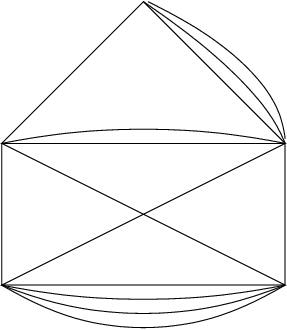
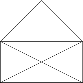
Figure 1: A multi-graph $G$ and its spanning subgraph $\tilde{G}$
4.

The number of components of a graph $G$ is $k(G)$ . If $V$ is apparend from the context and $G=(V,E)$ we set $k(E):=k(G)$ .
5.

The Tutte polynomial of a multi-graph $G$ (see e.g. [Bol98])

$\displaystyle T_{G}(x,y)$ $\displaystyle:=$ $\displaystyle\sum_{F\subseteq E}(x-1)^{k(F)-k(E)}(y-1)^{|F|-|V|+k(F)}$

2.1.1 The Tutte polynomial and the Jones polynomial for alternating links

Let $K$ be an alternating link with an alternating plane projection $P(K)$ . The region of the projection can be colored with 2 colors, say, purple and gold, such that two adjacent faces have different colors.

Two graphs are assigned to the projection, one corresponding to the purple colored regions and one to the golden regions. Every region gives rise to a vertex in the graph and two vertices are connected by an edge if the corresponding regions are adjacent to a common crossing. These graphs are called checkerboard graphs.

Each edge comes with a sign as in Figure 2.

Refer to caption — Figure 2: A positive or negative sign for the shaded region in the checkerboard graph

For an alternating link $K$ all edges are either positive or negative. Thus we have a positive checkerboard graph and a negative checkerboard graph. These two graphs are dual to each other. Let $G$ be the positive checkerboard graph, $a$ be the number of vertices in $G$ and $b$ be the number of vertices in the negative checkerboard graph.

It is well known, e.g. [Bol98], that the Jones Polynomial of an alternating link $K$ with positive checkerboard graph $G$ satisfies:

V_{K}(t)=(-1)^{w}t^{(b-a+3w)/4}T_{G}(-t,-1/t).

Here, $w$ is the writhe number, i.e. the algebraic crossing number of the link projection.

Since we are interested in the absolute values of coefficients of the Jones polynomial, all information relevant to us is contained in the evaluation $T_{G}(-t,-1/t)$ of the Tutte polynomial.

2.2 Reduction of multiple edges to simple edges

Our first step is to reduce the computation of the Tutte polynomial of a multi-graph to the computation of a weighted Tutte polynomial of a spanning simple graph.

Again, for a graph $G=(V,E)$ we denote by $\tilde{G}=(V,\tilde{E})$ a spanning simple graph. If $G$ is connected graph $G$ without vertices of valency $1$ , i.e. without loops then:

$\displaystyle T_{G}(-t,-1/t)$	$\displaystyle=$	$\displaystyle\sum_{F\subseteq E}(-t-1)^{k(F)-1}\left(-\frac{1}{t}-1\right)^{\|F\|-\|V\|+k(F)}$
	$\displaystyle=$	$\displaystyle\sum_{\tilde{F}\subseteq\tilde{E}}(-t-1)^{k(\tilde{F})-1}\left(-\frac{1}{t}-1\right)^{-\|V\|+k(\tilde{F})}\times$
		$\displaystyle\left(\sum_{\stackrel{{\scriptstyle r(e_{1})=1,\dots,r(e_{j})=1}}{{e_{1},\dots,e_{j}\in\tilde{F}}}}^{\mu(e_{1}),\dots,\mu(e_{j})}{\mu(e_{1})\choose r(e_{1})}\cdots{\mu(e_{j})\choose r(e_{j})}\left(-\frac{1}{t}-1\right)^{r(e_{1})+\dots+r(e_{j})}\right)$
	$\displaystyle=$	$\displaystyle\sum_{\tilde{F}\subseteq\tilde{E}}\left((-t-1)^{k(\tilde{F})-1}\left(-\frac{1}{t}-1\right)^{-\|V\|+k(\tilde{F})}\prod_{e\in\tilde{F}}\left(\left(-\frac{1}{t}\right)^{\mu(e)}-1\right)\right).$

So, with

	$\displaystyle P(m)$	$\displaystyle:=$	$\displaystyle\frac{\left(\left(-\frac{1}{t}\right)^{m}-1\right)}{\left(-\frac{1}{t}-1\right)}$
		$\displaystyle=$	$\displaystyle 1-t^{-1}+t^{-2}-\dots\pm t^{-m+1}$

we have

\displaystyle T_{G}(-t,-1/t)

\displaystyle=

\displaystyle\sum_{\tilde{F}\subseteq\tilde{E}}\left((-t-1)^{k(\tilde{F})-1}\left(-\frac{1}{t}-1\right)^{|\tilde{F}|-|V|+k(\tilde{F})}\prod_{e\in\tilde{F}}P(\mu(e))\right).

(1)

2.3 The highest terms of $T_{G}(-t,-1/t)$

Proposition 2.1.

Let $G=(V,E)$ be a planar multi-graph with spanning simple graph $\tilde{G}=(V,\tilde{E})$ . Let the Tutte Polynomial evaluation

T_{G}(-t,-1/t)=a_{n}t^{n}+a_{n+1}t^{n+1}+\dots+a_{m-1}t^{m-1}+a_{m}t^{m},

for suitable $n$ and $m$ .

Then the coefficients of the highest degree terms of $T_{G}(-t,-1/t)$ are:

1.

The highest degree term $t^{m}$ of $T_{G}(-t,-1/t)$ in $t$ is $t^{|V|-1}$ with coefficient

$a_{m}=(-1)^{|V|-1}.$
2.

The second highest degree term is $t^{|V|-2}$ with coefficient:

$a_{m-1}=(-1)^{|V|-1}\left(|V|-1-|\tilde{E}|\right).$

Note that $|a_{m-1}|=|\tilde{E}|+1-|V|$ .
3.

The third highest degree term is $t^{|V|-3}$ with coefficient:

$(-1)^{|V|}\left(-{|V|-1\choose 2}+(|V|-2)|\tilde{E}|-n(2)-{|\tilde{E}|\choose 2}+\mbox{tri}\right),$

where tri is the number of triangles in $\tilde{E}$ .

This term equals

$a_{m-2}=(-1)^{|V|}\left(-{|a_{m-1}|+1\choose 2}-n(2)+\mbox{tri}\right)$

Proof.

It is easy to see that $|\tilde{F}|-|V|+k(F)\geq 0$ for all $F$ .

Therefore,

\left(-\frac{1}{t}-1\right)^{|\tilde{F}|-|V|+k(F)}\prod_{e\in\tilde{F}}P(\mu(e))=\pm 1+\mbox{ higher terms in }t^{-1}

This means to determine the highest terms of $T_{G}(-t,-1/t)$ we have to analyze terms where $k(\tilde{F})$ is large.

Case: $k(\tilde{F})=|V|$ .

This means: $|\tilde{F}|=0.$ Thus the contribution in the sum in (1) is:

(-t-1)^{|V|-1}=(-1)^{|V|-1}\left(t^{|V|-1}+(|V|-1)\,t^{|V|-2}+{|V|-1\choose 2}\,t^{|V|-3}+\dots+1\right)

-

Case: $k(\tilde{F})=|V|-1$ .

This means: $|\tilde{F}|=1.$ Thus the contribution is:

$(-t-1)^{|V|-2}\,\sum_{e\in\tilde{E}}P(\mu(e))$

Recall our notation: For $G$ a multi-graph $n(j)$ is the number of edges in $\tilde{E}$ of multiplicity $\geq j$ . In particular $n(1)=|\tilde{E}|$

Thus

$\sum_{e\in\tilde{E}}P(\mu(e))=|\tilde{E}|-n(2)t^{-1}+n(3)t^{-2}-n(4)t^{-3}+\dots.$

Case: $k(\tilde{F})=|V|-2$ .

In this case either $|\tilde{F}|=2$ or $|\tilde{F}|=3$ and $\tilde{F}$ is a triangle. Thus the contribution is:

	$\displaystyle\sum_{e,f\in\tilde{E}}(-t-1)^{\|V\|-3}\,P(\mu(e))\,P(\mu(f))+$
	$\displaystyle\sum_{\stackrel{{\scriptstyle e,f,g\in\tilde{E}}}{{(e,f,g)\,\mbox{\tiny triangle}}}}(-t-1)^{\|V\|-3}\left(-\frac{1}{t}-1\right)P(\mu(e))P(\mu(f))P(\mu(g))$

By combining these computations we get the result. ∎

3 An Algebraic Point of View

It is interesting to formulate the results of Proposition 2.1 in a purely algebraic way:

Let $G$ be a multi-graph and $A$ it’s $N\times N$ adjacency matrix. Define a matrix $\tilde{A}$ to be the matrix that we get from $A$ by replacing every non-zero entry $A$ by $1$ . Thus, $\tilde{A}$ has only $1$ and $0$ as entries. Furthermore, $n(2)$ is half the number of entries in $A$ that are $\geq 2$ .

Then:

Corollary 3.1.

Let

T_{G}(-t,-1/t)=a_{n}t^{n}+a_{n+1}t^{n+1}+\dots+a_{m-1}t^{m-1}+a_{m}t^{m},

be the Jones evaluation of the Tutte Polynomial of a planar graph $G$ .

Then:

$\displaystyle\|a_{m}\|$	$\displaystyle=$	$\displaystyle 1$
$\displaystyle\|a_{m-1}\|$	$\displaystyle=$	$\displaystyle\frac{1}{2}\mbox{ trace }{\tilde{A}}^{2}-1-N$
$\displaystyle\|a_{m-2}\|$	$\displaystyle=$	$\displaystyle{\|a_{m-1}\|+1\choose 2}+n(2)-\frac{1}{6}\mbox{ trace }\tilde{A}^{3}$

Proof.

This is an immediate consequence of Proposition 2.1 together with the well-known results that for an adjacency matrix $A$ the number of edges is $\frac{1}{2}\mbox{ trace }A^{2}$ and the number of triangles is $\frac{1}{6}\mbox{ trace }A^{3}$ (see e.g [Big93]). ∎

4 Twist number and the Volume of an hyperbolic alternating knot

For a reference on hyperbolic structures on knot complements we refer e.g. to [CR98]. The figure eight knot has minimal volume among all hyperbolic knot complements [CM01]. Moreover, for a hyperbolic knot $K$ with crossing number $c>4$ by a result of Colin Adams (see [CR98]), the hyperbolic volume of its complement is bounded from above by

Vol(S^{3}-K)\leq(4c-16)v_{0},

where $v_{0}$ is the volume of a regular ideal hyperbolic tetrahedron.

For alternating knot complements a better general upper bound is known in terms of the twist number. As shown by Bill Menasco [Men84] a non-torus alternating knot is hyperbolic.

The twist number of a diagram of an alternating knot is the minimal number of twists (see Figure 3) in it. Here, a twist can consist of a single crossing. For example, the diagram of the knot in Figure 4 has twist number 8.

A twist corresponds to parallel edges in one of the checkerboard graphs. Let $D$ be a diagram for an alternating knot $K$ , $G=(V,E)$ be one of the two checkerboard graphs and let $G^{*}=(V^{*},E^{*})$ be the other, which is dual to $G$ . In particular, $|E|=|E^{*}|$ . As above we denote by $\tilde{G}=(V,\tilde{E})$ the reduced (simple) graph and by $\tilde{G}^{*}=(V^{*},\tilde{E}^{*})$ the reduced graph of the dual graph.

We can now define the twist number by

$\displaystyle T(K)$	$\displaystyle:=$	$\displaystyle\|E\|-(\|E\|-\|\tilde{E}\|)-(\|E^{}\|-\|\tilde{E}^{}\|)$
	$\displaystyle=$	$\displaystyle\|E\|-(\|E\|-\|\tilde{E}\|)-(\|E\|-\|\tilde{E}^{*}\|)$
	$\displaystyle=$	$\displaystyle\|\tilde{E}\|+\|\tilde{E}^{*}\|-\|E\|.$

It is an easy exercise to see that

1.

$T(K)$ is indeed realized as the twist number of a diagram of $K$ .
2.

$T(K)$ is an invariant of all alternating projections of $K$ . This follows from the Tait-Menasco-Thistlethwaite flyping theorem [MT93]. Below we will give a different argument for it.

Theorem 4.1 (Lackenby [Lac00], Agol, D. Thurston).

v_{0}\,(T(K)-2)\leq Vol(S^{3}-K)<10v_{0}(T(K)-1),

where $Vol(S^{3}-K)$ is the hyperbolic Volume and $v_{0}$ is the volume of an ideal regular hyperbolic tetrahedron.

5 Coefficients of the Jones polynomial

For an alternating knot $K$ with reduced alternating diagram $D$ with $c$ crossings it holds [Thi87, Kau87, Mur87]:

1.

The span of the Jones polynomial is $c$ .
2.

The signs of the coefficients are alternating
3.

The absolute values of the highest and lowest coefficients are $1$ .

Proposition 2.1 immediately leads to:

Theorem 5.1.

Let $V_{K}(t)=a_{n}t^{n}+a_{n+1}t^{n+1}+\dots+a_{m}t^{m}$ be the Jones polynomial of an alternating knot $K$ and let $G=(V,E)$ be a checkerboard graph of a reduced alternating projection of $K$ .

Then

1.

$|a_{n}|=|a_{m}|=1$
2.

$|a_{n+1}|+|a_{m-1}|=T(K)$
3.

$|a_{n+2}|+|a_{m-2}|+|a_{m-1}||a_{n+1}|=\frac{T(K)+T(K)^{2}}{2}+n(2)+n^{*}(2)-\mbox{tri}-\mbox{tri}^{*},$

where $n(2)$ is the number of edges in $\tilde{E}$ of multiplicity $>1$ and $n^{*}(2)$ the corresponding number in the dual checkerboard graph.

The number tri is the number of triangles in the graph $\tilde{G}=(V,\tilde{E})$ and $\mbox{tri}^{*}$ corresponds to tri in the dual graph.
4.

In particular, the twist number is an invariant of reduced alternating projections of the knot.

Proof.

Let $K$ be an alternating knot with a reduced alternating diagram $D$ having a checkerboard graph $G=(V,E)$ and dual graph $G^{*}=(V^{*},E^{*})$ .

We have:

|E|=|E^{*}|\quad\mbox{ and }\quad|V|+|V^{*}|=|E|+2.

Recall, that the twist number $T(K)$ of $K$ is defined as:

$\displaystyle T(K)$	$\displaystyle:=$	$\displaystyle\|E\|-(\|E\|-\|\tilde{E}\|)-(\|E\|-\|\tilde{E^{*}}\|)$
	$\displaystyle=$	$\displaystyle\|\tilde{E}\|+\|\tilde{E^{*}}\|-\|E\|$
	$\displaystyle=$	$\displaystyle(\|\tilde{E}\|-\|V\|+1)+(\|\tilde{E^{}}\|-\|V^{}\|+1)$

The identities now follow from Proposition 2.1. ∎

Volume-ish Theorem. For an alternating, prime, non-torus knot $K$ let

V_{K}(t)=a_{n}t^{n}+\dots+a_{m}t^{m}

be the Jones polynomial of $K$ . Then

2v_{0}(\max(|a_{m-1}|,|a_{n+1}|)-1)\leq\mbox{Vol}(S^{3}-K)\leq 10v_{0}(|a_{n+1}|+|a_{m-1}|-1).

Here, $v_{0}\approx 1.0149416$ is the Volume of an ideal regular hyperbolic tetrahedron.

Proof.

The upper bound follows from Theorem 4.1 and Theorem 5.1. For the lower bound we need a closer look at [Lac00].

We can suppose that $K$ admits a diagram such that both checkerboard graphs are inbedded so that every pair of edges connecting the same two vertices are adjacent to each other in the plane. This can be done by flypes.

Suppose $G_{p}=(V_{p},E_{p})$ is the positive (colored in purple) and $G_{g}=(V_{g},E_{g})$ is the negative (colored in gold) checkerboard graph. Since $G_{p}^{*}=G_{g}$ we have $|E_{p}|=|E_{g}|$ and

|V_{p}|-|E_{p}|+|V_{g}|=2=|V_{p}|-|E_{g}|+|V_{g}|.

Set $r_{p}$ (resp. $r_{g}$ ) to be the number of vertices in $G_{p}$ (resp. $G_{g}$ ) of valency at least $3$ .

In 4.1 it is proved, using results of Ian Agol that

\mbox{Vol}(S^{3}-K)\geq 2v_{0}(\max(r_{p},r_{g})-2).

If $\tilde{G}_{p}=(V_{p},\tilde{E}_{p})$ and $\tilde{G}_{g}=(V_{g},\tilde{E}_{g})$ are the reduced graphs of $G_{p}$ and $G_{g}$ than it is easy to see that

$\displaystyle r_{p}$	$\displaystyle=$	$\displaystyle\|V_{p}\|-(\|E_{g}\|-\|\tilde{E}_{g}\|)$
	$\displaystyle=$	$\displaystyle 2-\|V_{g}\|+\|\tilde{E}_{g}\|$
	$\displaystyle=$	$\displaystyle\|a_{n+1}\|+1.$

Similarily, $r_{g}=|a_{m-1}|+1$ and the lower bound follows. ∎

5.1 Example

The checkerboard graph $G$ of the knot in Figure 4 has $|V|=8$ vertices, $|\tilde{E}|=11,n(2)=2$ and $tri=1$ .

It’s dual has $|V^{*}|=7$ vertices, $|\tilde{E^{*}}|=10,n^{*}(2)=3$ and $tri^{*}=2$ .

Therefore, with the above notation for the coefficients of the Jones polynomial,

$\displaystyle\|a_{n}\|$	$\displaystyle=$	$\displaystyle 1$
$\displaystyle\|a_{n+1}\|$	$\displaystyle=$	$\displaystyle\|\tilde{E}\|+1-\|V\|=4$
$\displaystyle\|a_{n+2}\|$	$\displaystyle=$	$\displaystyle{\|a_{n+1}\|+1\choose 2}+n(2)-tri=10+2-1=11$
$\displaystyle\|a_{m}\|$	$\displaystyle=$	$\displaystyle 1$
$\displaystyle\|a_{m-1}\|$	$\displaystyle=$	$\displaystyle\|\tilde{E^{}}\|+1-\|V^{}\|=4$
$\displaystyle\|a_{m-2}\|$	$\displaystyle=$	$\displaystyle{\|a_{m-1}\|+1\choose 2}+n^{}(2)-tri^{}=10+3-2=11$

The complete Jones polynomial of the knot is, according to Knotscape:

	$\displaystyle V_{13.121}(t)$	$\displaystyle=$	$\displaystyle t^{-12}-4t^{-11}+11t^{-10}-23t^{-9}+35t^{-8}-47t^{-7}+53t^{-6}$
			$\displaystyle-52t^{-5}+47t^{-4}-34t^{-3}+22t^{-2}-11t^{-1}+4-t$

and the hyperbolic volume is

\mbox{Vol}(S^{3}-K)\approx 21.1052106828.

Appendix A Higher twist numbers of prime alternating knots on $14$ crossings

In this appendix we give experimental data on the relationsship of the twist number, as computed using the Jones polynomial, and the hyperbolic volume of knots. All data are taken from Knotscape, written by Jim Hoste, Morwen Thistlethwaite and Jeff Weeks [HTW98]. We confined ourselves to knots with crossing number 14. As before, let $V_{K}(t)=a_{n}t^{n}+a_{n+1}t^{n+1}+\dots+a_{m}t^{m}$ be the Jones polynomial of an alternating prime knot $K$ .

As shown, the twist number is $T(K)=|a_{n+1}|+|a_{m-1}|$ . We call $T_{i}(K)=|a_{n+i}|+|a_{m-i}|$ the higher “twist” numbers. In particular, $T(L)=T_{1}(L)$ .

Appendix B Higher “twist numbers” of prime non-alternating knots on $14$ crossings

For non-alternating knots we keep the notation, although there is no direct geometrical justification known:

Again, let $V_{L}(t)=a_{n}t^{n}+a_{n+1}t^{n+1}+\dots+a_{m}t^{m}$ be the Jones polynomial of a non-alternating knot $L$ .

Define the twist number is $T(L)=|a_{n+1}|+|a_{m-1}|$ . As in the alternating case, we call $T_{i}(L)=|a_{n+i}|+|a_{m-1}|$ the higher twist numbers. In particular, $T(L)=T_{1}(L)$ .

If the knot is non-hyperbolic we set its volume = 0.

The pictures give, for non-alternating knots with crossing number 14, the relation between the twist number and the Volume, resp. the number $T_{2},T_{3},T_{4}$ and the volume.

References

[Big93] Norman Biggs, Algebraic graph theory, second ed., Cambridge Mathematical Library, Cambridge University Press, Cambridge, 1993. MR 95h:05105
[BNG96] D. Bar-Natan and S. Garoufalidis, On the Melvin-Morton-Rozansky conjecture, Invent. Math. 125 (1996), no. 1, 103–133. MR 97i:57004
[Bol98] Béla Bollobás, Modern graph theory, Graduate Texts in Mathematics, vol. 184, Springer-Verlag, New York, 1998. MR 99h:05001
[Chm98] S. Chmutov, A proof of the Melvin-Morton conjecture and Feynman diagrams, J. Knot Theory Ramifications 7 (1998), no. 1, 23–40. MR 99c:57012
[CM01] Chun Cao and G. Robert Meyerhoff, The orientable cusped hyperbolic $3$ -manifolds of minimum volume, Invent. Math. 146 (2001), no. 3, 451–478. MR 2002i:57016
[CR98] P. J. Callahan and A. W. Reid, Hyperbolic structures on knot complements, Chaos Solitons Fractals 9 (1998), no. 4-5, 705–738, Knot theory and its applications. MR 99e:57022
[DH97] Oliver T. Dasbach and Stefan Hougardy, Does the Jones Polynomial Detect Unknottedness?, Experimental Math. 6 (1997), no. 1, 51 – 56.
[HTW98] Jim Hoste, Morwen Thistlethwaite, and Jeff Weeks, The first 1,701,936 knots, Math. Intelligencer 20 (1998), no. 4, 33–48. MR 99i:57015
[Kau87] Louis H. Kauffman, State models and the Jones polynomial, Topology 26 (1987), no. 3, 395–407. MR 88f:57006
[Lac00] Marc Lackenby, The volume of hyperbolic alternating link complements, to appear in Proc. London Math. Soc., 2000.
[LW01] Xiao-Song Lin and Zhenghan Wang, Random walk on knot diagrams, colored Jones polynomial and Ihara-Selberg zeta function, Knots, braids, and mapping class groups—papers dedicated to Joan S. Birman (New York, 1998), AMS/IP Stud. Adv. Math., vol. 24, Amer. Math. Soc., Providence, RI, 2001, pp. 107–121. MR 2003f:57026
[Men84] William W. Menasco, Closed incompressible surfaces in alternating knot and link complements, Topology 23 (1984), no. 1, 37–44. MR 86b:57004
[MM01] Hitoshi Murakami and Jun Murakami, The colored Jones polynomials and the simplicial volume of a knot, Acta Math. 186 (2001), no. 1, 85–104. MR 2002b:57005
[MT93] William W. Menasco and Morwen B. Thistlethwaite, The classification of alternating links, Ann. of Math. (2) 138 (1993), no. 1, 113–171. MR 95g:57015
[Mur87] Kunio Murasugi, Jones polynomials and classical conjectures in knot theory, Topology 26 (1987), no. 2, 187–194. MR 88m:57010
[Thi87] Morwen B. Thistlethwaite, A spanning tree expansion of the Jones polynomial, Topology 26 (1987), no. 3, 297–309. MR 88h:57007
[Vai97] Arkady Vaintrob, Melvin-Morton conjecture and primitive Feynman diagrams, Internat. J. Math. 8 (1997), no. 4, 537–553. MR 99b:57027

$\displaystyle\|a_{n}\|$	$\displaystyle=$	$\displaystyle 1$
$\displaystyle\|a_{n+1}\|$	$\displaystyle=$	$\displaystyle\|\tilde{E}\|+1-\|V\|=4$
$\displaystyle\|a_{n+2}\|$	$\displaystyle=$	$\displaystyle{\|a_{n+1}\|+1\choose 2}+n(2)-tri=10+2-1=11$
$\displaystyle\|a_{m}\|$	$\displaystyle=$	$\displaystyle 1$
$\displaystyle\|a_{m-1}\|$	$\displaystyle=$	$\displaystyle\|\tilde{E^{}}\|+1-\|V^{}\|=4$
$\displaystyle\|a_{m-2}\|$	$\displaystyle=$	$\displaystyle{\|a_{m-1}\|+1\choose 2}+n^{}(2)-tri^{}=10+3-2=11$

A volume-ish theorem for the Jones polynomial of alternating knots

Abstract

1 Introduction

2 The Jones Polynomial evaluation of the Tutte Polynomial

2.1 Notations

2.1.1 The Tutte polynomial and the Jones polynomial for alternating links

2.2 Reduction of multiple edges to simple edges

2.3 The highest terms of TG(−t,−1/t)T_{G}(-t,-1/t)

Proposition 2.1.

Proof.

3 An Algebraic Point of View

Corollary 3.1.

Proof.

4 Twist number and the Volume of an hyperbolic alternating knot

Theorem 4.1 (Lackenby [Lac00], Agol, D. Thurston).

5 Coefficients of the Jones polynomial

Theorem 5.1.

Proof.

Proof.

5.1 Example

Appendix A Higher twist numbers of prime alternating knots on 1414 crossings

Appendix B Higher “twist numbers” of prime non-alternating knots on 1414 crossings

References

A volume-ish theorem for the Jones polynomial
of alternating knots

2.3 The highest terms of $T_{G}(-t,-1/t)$

Appendix A Higher twist numbers of prime alternating knots on $14$ crossings

Appendix B Higher “twist numbers” of prime non-alternating knots on $14$ crossings