Chebyshev Series Expansion of Inverse Polynomials

Richard J. Mathar Address: Sterrewacht, Universiteit Leiden, Postbus 9513, 2300 RA Leiden, The Netherlands Email address: mathar@strw.leidenuniv.nl

Date: August 11, 2026

Abstract.

An inverse polynomial has a Chebyshev series expansion

1/\sum_{j=0}^{k}b_{j}T_{j}(x)=\mathop{{\sum}^{\prime}}_{n=0}^{\infty}a_{n}T_{n}(x)

if the polynomial has no roots in $[-1,1]$ . If the inverse polynomial is decomposed into partial fractions, the $a_{n}$ are linear combinations of simple functions of the polynomial roots. Also, if the first $k$ of the coefficients $a_{n}$ are known, the others become linear combinations of these with expansion coefficients derived recursively from the $b_{j}$ ’s. On a closely related theme, finding a polynomial with minimum relative error towards a given $f(x)$ is approximately equivalent to finding the $b_{j}$ in $f(x)/\sum_{0}^{k}b_{j}T_{j}(x)=1+\sum_{k+1}^{\infty}a_{n}T_{n}(x)$ , and may be handled with a Newton method providing the Chebyshev expansion of $f(x)$ is known.

Key words and phrases:

Chebyshev series, orthogonal polynomials, approximation

2000 Mathematics Subject Classification

Primary 33C45, 42C20; Secondary 41A50, 41A10; Tertiary 65D15

1. Introduction and Scope

The Chebyshev polynomials $T_{n}(x)$ are even or odd functions of $x$ defined as [1, (22.3.6)][3, (3.6)]

(1.1)

T_{0}(x)=1,\quad T_{n}(x)=\frac{n}{2}\sum_{m=0}^{\lfloor n/2\rfloor}(-)^{m}\frac{(n-m-1)!}{m!(n-2m)!}(2x)^{n-2m},\quad n=1,2,3\ldots

where the Gauss bracket $\lfloor.\rfloor$ denotes the largest integer not greater than the number it embraces. The reverse formula is [7, p. 412][13, p. 52][14]

(1.2)

x^{n}=2^{1-n}{\mathop{{\sum}^{\prime}}_{\genfrac{}{}{0.0pt}{}{j=0}{n-j \text{even}}}^{n}}\binom{n}{(n-j)/2}T_{j}(x)

where the prime at the sum symbol means the first term (at $j=0$ and even $n$ ) is to be halved. The polynomials are orthogonal over the interval $[-1,1]$ with weight function $1/\sqrt{1-x^{2}}$ [1, (22.2.4)][7, (4.2)][2]

(1.3)

\int_{-1}^{1}T_{n}(x)T_{m}(x)\frac{dx}{\sqrt{1-x^{2}}}=\left\{\begin{array}[]{c@{,\quad}c}\pi&n=m=0,\\ \pi/2&n=m\neq 0,\\ 0&n\neq m.\\ \end{array}\right.

The product rule is [1, (22.7.24)][16, (A.1)][14, (2.10)]

(1.4)

T_{n}(x)T_{m}(x)=\frac{1}{2}\left(T_{|m-n|}(x)+T_{m+n}(x)\right).

The indefinite integral is [7, (4.8)][13, p. 54][14, (2.12)]

(1.5)

\int T_{n}(x)dx=\left\{\begin{array}[]{ll}T_{1}(x),&n=0,\\ \frac{1}{4}T_{2}(x),&n=1,\\ \frac{1}{2}\left(\frac{T_{n+1}(x)}{n+1}-\frac{T_{n-1}(x)}{n-1}\right),&n>1,\\ \end{array}\right.

which correlates to the derivative

(1.6)

\frac{d}{dx}T_{n}(x)=2n\mathop{{\sum}^{\prime}}_{\genfrac{}{}{0.0pt}{}{l=0}{n-l\, \text{odd}}}^{n-1}T_{l}(x).

The expansion of an inverse polynomial of degree $k$ in a power series is [1, (3.6.16)]

(1.7)

\frac{1}{\sum_{j=0}^{k}d_{j}x^{j}}=\sum_{n=0}^{\infty}c_{n}x^{n},

with recursively accessible [15, 0.313]

(1.8)

c_{n}=-\frac{1}{d_{0}}\sum_{\genfrac{}{}{0.0pt}{}{j=0}{n-j\le k}}^{n-1}d_{n-j}c_{j},\quad c_{0}=\frac{1}{d_{0}},\quad n\geq 1.

The topic of this script is the equivalent arithmetic expansion of the inverse polynomial in a Chebyshev series,

(1.9)

\frac{1}{\sum_{j=0}^{k}d_{j}x^{j}}=\frac{1}{\sum_{j=0}^{k}b_{j}T_{j}(x)}={\mathop{{\sum}^{\prime}}_{n=0}^{\infty}}a_{n}T_{n}(x),

i.e., computation of the coefficients

(1.10)

a_{n}=\frac{2}{\pi}\int_{-1}^{1}\frac{T_{n}(x)}{\sum_{j=0}^{k}b_{j}T_{j}(x)}\frac{dx}{\sqrt{1-x^{2}}}

given the sets { $b_{j}$ } or { $d_{j}$ } that define the original function. Both sets are related via [30, (3)][31, (37)] and with (1.1) via

(1.11)

d_{l}=\frac{2^{l-1}}{l!}\sum_{\genfrac{}{}{0.0pt}{}{j=0}{j-l \text{even}}}^{k}(-)^{(j-l)/2}j\frac{(\frac{j+l}{2}-1)!}{(\frac{j-l}{2})!}b_{j},\quad l=0,\ldots,k.

The expansion (1.9) exists if the inverse polynomial is bound in the interval $[-1,1]$ , i.e., if $\sum d_{j}x^{j}$ has no roots in $[-1,1]$ .

Characteristic generic methods of evaluating (1.10) are not reviewed here: (i) Fourier transform methods [7, (4.7)][6, 12, 10], (ii) sampling with Gauss-type quadratures [1, (25.4.38)][25, 33, 20] which effectively means using an implicit intermediate interpolatory polynomial to represent $1/\sum_{j=0}^{k}b_{j}T_{j}(x)$ , (iii) approximation by truncation of (1.7), then insertion of (1.2), (iv) using the near-minimax properties of the Chebyshev series [23, 21].

Remark 1.1.

The Fourier-Chebyshev series [18, 27][28, (3.4.1f)]

(1.12)

\frac{T_{n}(z)-tT_{|n-m|}(z)}{1-2tT_{m}(z)+t^{2}}=\sum_{k=0}^{\infty}T_{km+n}(z)t^{k}

provides special cases of polynomials with particularly simple expansions.

Remark 1.2.

Insertion of $n=1$ in (1.4) shows that the coefficients of

(1.13)

f(x)=\mathop{{\sum}^{\prime}}_{n=0}^{\infty}f_{n}T_{n}(x)

and

(1.14)

\frac{f(x)}{x}=\mathop{{\sum}^{\prime}}_{n=0}^{\infty}g_{n}T_{n}(x)

are related as

(1.15)

f_{0}=g_{1},\quad 2f_{n-1}=g_{n-2}+g_{n},\quad n\geq 2.

Chapter 2 explains how the $a_{n}$ of (1.10) could be computed supposed the inverse polynomial has been decomposed into partial fractions. Chapter 3 provides a recursive algorithm to derive high-indexed $a_{n}$ ( $n\geq k$ ) supposed the low-indexed $a_{n}$ are given by other means. Chapter 4 touches on a (standard) integral-free method to compute approximate low-indexed $a_{n}$ , and Chapter 5 deals with a specific inverse problem —which is finding the $b_{j}$ from partially known $a_{n}$ —related to polynomial approximants with minimum relative error.

2. The Case of Known Partial Fractions

The straight way of computing the Chebyshev series uses the decomposition of $1/\sum d_{j}x^{j}$ into partial fractions [15, 2.102], which reduces (1.9) to the calculation of the $a_{n,s}$ in

(2.1)

\frac{1}{(z-x)^{s}}\equiv\mathop{{\sum}^{\prime}}_{n=0}^{\infty}a_{n,s}(z)T_{n}(x),

where $z$ is a root of the polynomial,

(2.2)

\sum_{j=0}^{k}d_{j}z^{j}=0.

Sign flips of $z$ and $x$ in (2.1) show that

(2.3)

a_{n,s}(-z)=(-)^{n+s}a_{n,s}(z).

The case of $s=1$ has been evaluated earlier [17, (A.6)][27, 32] based on [1, (22.9.9)][35, (18)],

(2.4)

a_{n,1}(z)=\frac{2}{(z^{2}-1)^{1/2}}\frac{1}{w^{n}},\quad w\equiv z+(z^{2}-1)^{1/2},\quad z\notin[-1,1].

The branch cuts of $(z^{2}-1)^{1/2}$ must be chosen such that $|w|>1$ .

Example 2.1.

(2.5)

\frac{1}{1+x^{2}}=\frac{i}{2}\frac{1}{i-x}-\frac{i}{2}\frac{1}{-i-x}

consists of two terms,

(2.6)

a_{n,1}(i)=-\frac{\sqrt{2}i^{1-n}}{(1+\sqrt{2})^{n}},\quad a_{n,1}(-i)=(-)^{n}\frac{\sqrt{2}i^{1-n}}{(1+\sqrt{2})^{n}},

which recombine with the two factors $i/2$ and $-i/2$ to [28, (3.4.1a)]

(2.7)

\frac{1}{1+x^{2}}=\sqrt{2}\mathop{{\sum}^{\prime}}_{n=0,2,4,6,\ldots}\frac{(-)^{n/2}}{(1+\sqrt{2})^{n}}T_{n}(x).

Remark 2.2.

The shifted Chebyshev polynomials $T^{*}(x)\equiv T(2x-1)$ are orthogonal over $[0,1]$ with weight $1/\sqrt{x(1-x)}$ [1, (22.2.8)][26]. From (2.1) we get

(2.8)

\frac{1}{(z-x)^{s}}=2^{s}\mathop{{\sum}^{\prime}}_{n=0}^{\infty}a_{n,s}(2z-1)T_{n}^{*}(x),

and (1.5) becomes

(2.9)

\int T_{n}^{*}(x)dx=\left\{\begin{array}[]{ll}\frac{1}{2}T_{1}^{*}(x),&n=0,\\ \frac{1}{8}T_{2}^{*}(x),&n=1,\\ \frac{1}{4}\left(\frac{T_{n+1}^{*}(x)}{n+1}-\frac{T_{n-1}^{*}(x)}{n-1}\right),&n>1.\\ \end{array}\right.

Example 2.3.

An example of $s=1$ , $z=-1$ in (2.8) is

(2.10)

\frac{1}{1+x}=-\frac{1}{-1-x}=-2\mathop{{\sum}^{\prime}}_{n=0}^{\infty}a_{n,1}(-3)T_{n}^{*}(x),

where

(2.11)

a_{n,1}(-3)=\frac{(-)^{n+1}}{\sqrt{2}(3+2\sqrt{2})^{n}}

according to (2.4).

Higher second indices $s$ of the $a_{n,s}$ are obtained from (2.1) by repeated derivation w.r.t. $z$ ,

(2.12)

(-)^{s}s!\frac{1}{(z-x)^{s+1}}={\mathop{{\sum}^{\prime}}_{n=0}^{\infty}}\left(\frac{\partial}{\partial z}\right)^{s}a_{n,1}(z)T_{n}(x),

via [15, 0.432.1],

(2.13)		$\displaystyle a_{0,s+1}(z)$	$\displaystyle=$	$\displaystyle\frac{2}{s!}(-)^{s}\left(\frac{\partial}{\partial z}\right)^{s}\frac{1}{(z^{2}-1)^{1/2}}$
(2.13)			$\displaystyle=$	$\displaystyle 2\sum_{l=0}^{\lfloor s/2\rfloor}\frac{(-)^{l}}{l!(s-2l)!}\left(\frac{1}{2}\right)_{s-l}\frac{(2z)^{s-2l}}{(z^{2}-1)^{\frac{1}{2}+s-l}},\quad s\geq 0,$

with Pochhammer’s Symbol defined as [1, (6.1.22)]

(2.14)

(\alpha)_{k}\equiv\alpha(\alpha+1)(\alpha+2)\cdots(\alpha+k-1)=\Gamma(\alpha+k)/\Gamma(\alpha),\quad(\alpha)_{0}=1.

The formula

	$\displaystyle(s-1)\int\frac{dx}{(z-x)^{s}}$	$\displaystyle=$	$\displaystyle\frac{1}{(z-x)^{s-1}}+A_{s}$
		$\displaystyle=$	$\displaystyle(s-1)\mathop{{\sum}^{\prime}}_{n=0}^{\infty}a_{n,s}\int T_{n}(x)dx=\mathop{{\sum}^{\prime}}_{n=0}^{\infty}a_{n,s-1}T_{n}(x)+A_{s},\quad s\geq 2$

in conjunction with the method quoted by Cody [7, (4.8)][22, (25)] yields

(2.15)

a_{n+1,s}(z)=a_{n-1,s}(z)-\frac{2n}{s-1}a_{n,s-1}(z),\quad n\geq 1,\quad s\geq 2.

One needs (2.13) and

(2.16)		$\displaystyle a_{1,s+1}(z)$	$\displaystyle=$	$\displaystyle\frac{2}{\pi}\int_{-1}^{1}\frac{T_{1}(x)}{(z-x)^{s+1}}\frac{dx}{\sqrt{1-x^{2}}}$
(2.16)			$\displaystyle=$	$\displaystyle-a_{0,s}(z)+za_{0,s+1}(z)$

to start the recurrence (2.15) and to obtain all coefficients in (2.1) for a particular $z$ . Closed form expressions for solving these recurrences in terms of Legendre Polynomials of $z/\sqrt{z^{2}-1}=(w^{2}+1)/(w^{2}-1)$ have been given by Elliott [8].

Remark 2.4.

(2.16) may be generalized to

(2.17)

\frac{2}{\pi}\int_{-1}^{1}\frac{x^{l}}{(z-x)^{n}}\frac{dx}{\sqrt{1-x^{2}}}=\sum_{m=0}^{l}(-)^{m}\binom{l}{m}z^{l-m}a_{0,n-m},\quad l<n.

and with (1.2) and (1.4) to

(2.18)

\frac{2}{\pi}\int_{-1}^{1}\frac{x^{l}}{(z-x)^{n}}\frac{T_{s}(x)}{\sqrt{1-x^{2}}}dx=\frac{1}{2^{l}}\mathop{{\sum}^{\prime}}_{\genfrac{}{}{0.0pt}{}{i=0}{l-i \text{even}}}^{l}\binom{l}{\frac{l-i}{2}}\left[a_{|i-s|,n}+a_{i+s,n}\right].

Example 2.5.

An example of degree $k=3$ is

(2.19)		$\displaystyle\frac{1}{(4-x)^{2}(5+x)}$	$\displaystyle=$	$\displaystyle\frac{1}{78\frac{1}{2}T_{0}(x)-23\frac{1}{4}T_{1}(x)-1\frac{1}{2}T_{2}(x)+\frac{1}{4}T_{3}(x)}$
(2.20)			$\displaystyle=$	$\displaystyle\frac{1}{9}\frac{1}{(4-x)^{2}}+\frac{1}{81}\frac{1}{(4-x)}-\frac{1}{81}\frac{1}{(-5-x)}.$

The root at $z=4$ yields

(2.21)

a_{0,1}(4)=2/\sqrt{15}\approx 0.5164

from (2.4) and

(2.22)

a_{0,2}(4)=2\cdot\frac{1}{2}\cdot\frac{2\cdot 4}{\sqrt{15}^{3}}\approx 0.1377

from (2.13). The root at $z=-5$ yields

(2.23)

a_{0,1}(-5)=2/(-\sqrt{24})\approx-0.4082

from (2.4). The combined total in (2.20) is

(2.24)

a_{0}=\frac{2}{\pi}\int_{-1}^{1}\frac{1}{(4-x)^{2}(5+x)}\frac{dx}{\sqrt{1-x^{2}}}\approx\frac{1}{9}\cdot 0.1377+\frac{1}{81}\cdot 0.5164-\frac{1}{81}\cdot(-0.4082)\approx 0.0267.

Example 2.6.

A case of $k=\infty$ is [15, 1.421.2]

(2.25)

\frac{\tanh(\pi x/2)}{x}=\frac{4}{\pi}\sum_{m=1}^{\infty}\frac{i}{2(2m-1)}\left[\frac{1}{i(2m-1)-x}-\frac{1}{-i(2m-1)-x}\right].

The roots at $z=\pm i(2m-1)$ yield

(2.26)

a_{0,1}(z)=2/\left(\pm i\sqrt{4m^{2}-4m+2}\right),

and the combined total is

(2.27)

a_{0}=\frac{2}{\pi}\int_{-1}^{1}\frac{\tanh(\pi x/2)}{x}\frac{dx}{\sqrt{1-x^{2}}}=\frac{4}{\pi}\sum_{m=1}^{\infty}\frac{1}{(2m-1)\sqrt{m^{2}-m+1/2}}\approx 2.38.

Remark 2.7.

From (2.4)

(2.28)

\frac{\partial a_{n,1}(z)}{\partial z}=-a_{n,1}\left[\frac{z}{z^{2}-1}+\frac{n}{(z^{2}-1)^{1/2}}\right],

so the (linear) propagation of the absolute relative error in the root $z$ to the error in the coefficient $a_{n,1}$ is

(2.29)

\left|\frac{\Delta a_{n,1}}{a_{n,1}}\right|=\left|\frac{\Delta z}{z}\right|\cdot\left|\frac{z^{2}}{z^{2}-1}+\frac{nz}{(z^{2}-1)^{1/2}}\right|.

Remark 2.8.

An associated factorization $\sum_{j=0}^{k}b_{j}T_{j}(x)\propto\prod_{m=1}^{l}(z_{m}-x)^{s_{m}}$ , with $l$ different roots of multiplicities $s_{m}$ , decomposes the square root of the polynomial into a $l$ -fold product of series of the prototypical forms

(2.30)		$\displaystyle\sqrt{z-x}$	$\displaystyle=$	$\displaystyle\mathop{{\sum}^{\prime}}_{n=0}^{\infty}q_{n}(z)T_{n}(x),\quad s_{m}=1,$
(2.31)		$\displaystyle z-x$	$\displaystyle=$	$\displaystyle zT_{0}(x)-T_{1}(x),\quad s_{m}=2,$

where [15, 2.576.2]

(2.32)

q_{0}(z)=\frac{2}{\pi}\int_{0}^{\pi}dt\sqrt{z-\cos t}=\frac{4}{\pi}\sqrt{1+z}E(\frac{2}{1+z})

is related to Complete Elliptic Integrals of the Second Kind $E$ in the notation of [1, (17.3.4)]. The $q_{n}(z)$ with $n\geq 1$ follow recursively using [1, (17.1.4)]. In particular, one may expand $T_{n}(x)$ in terms of $P_{n}^{(0,-1/2)}(x)$ with [11, (1.4)] to obtain

(2.33)

q_{n}(1)=\frac{2^{5/2}}{\pi}\sum_{l=0}^{n}\frac{(-n)_{l}(n)_{l}}{(3/2)_{l}(1/2)_{l}},\quad n=0,1,2,\ldots

for the Chebyshev coefficients of $\sqrt{1-x}$ . See [29] for an application.

3. Recurrence of Expansion Coefficients

The $T_{n}$ in (1.10) may be decomposed into a unique product of a polynomial by the denominator plus a remainder of polynomial degree less than $k$ . [The dependence on $x$ is omitted at all $T_{n}(x)$ for brevity.]

(3.1)		$\displaystyle T_{n}$	$\displaystyle=$	$\displaystyle(d_{0}^{(n)}T_{0}+d_{1}^{(n)}T_{1}+\cdots+d_{n-k}^{(n)}T_{n-k})(b_{0}T_{0}+b_{1}T_{1}+\cdots+b_{k}T_{k})$
(3.1)				$\displaystyle+\frac{c_{0}^{(n)}}{2}T_{0}+c_{1}^{(n)}T_{1}+c_{2}^{(n)}T_{2}+\cdots+c_{k-1}^{(n)}T_{k-1}.$

Expansion with (1.4) yields a system of linear equations for the vector of the unknowns $d_{j}^{(n)}$ and $c_{j}^{(n)}$ :

(3.2)

\left(\begin{array}[]{ccccc@{|}ccccc}1&0&\ldots&\ldots&0&2b_{0}&b_{1}&b_{2}&b_{3}&\ldots\\ 0&1&0&\ldots&0&b_{1}&b_{0}+\frac{b_{2}}{2}&\frac{b_{1}+b_{3}}{2}&\frac{b_{2}+b_{4}}{2}&\ldots\\ \vdots&0&\ddots&\ddots&\vdots&b_{2}&\frac{b_{1}+b_{3}}{2}&b_{0}+\frac{b_{4}}{2}&\frac{b_{1}+b_{5}}{2}&\ldots\\ \vdots&\vdots&\ddots&1&0&\vdots&\vdots&\vdots&\vdots&\vdots\\ 0&\ldots&\ldots&0&1&b_{k-1}&\frac{b_{k-2}+b_{k}}{2}&\frac{b_{k-3}}{2}&\ldots&\ldots\\ \hline\cr 0&\ldots&\ldots&\ldots&0&b_{k}&\frac{b_{k-1}}{2}&\frac{b_{k-2}}{2}&\frac{b_{k-3}}{2}&\ldots\\ \vdots&\ldots&\ldots&\ldots&\vdots&0&\frac{b_{k}}{2}&\frac{b_{k-1}}{2}&\ldots&\ldots\\ \vdots&\ldots&\ldots&\ldots&\vdots&\vdots&0&\\ \vdots&\vdots&\vdots&\vdots&\vdots&\vdots&\vdots&\ddots&&\frac{b_{k-1}}{2}\\ 0&\ldots&\ldots&\ldots&0&0&\ldots&\ldots&0&\frac{b_{k}}{2}\\ \end{array}\right)\cdot\left(\begin{array}[]{c}c_{0}^{(n)}\\ c_{1}^{(n)}\\ \vdots\\ \vdots\\ c_{k-1}^{(n)}\\ \hline\cr d_{0}^{(n)}\\ d_{1}^{(n)}\\ \vdots\\ d_{n-k-1}^{(n)}\\ d_{n-k}^{(n)}\end{array}\right)=\left(\begin{array}[]{c}0\\ \vdots\\ \vdots\\ \vdots\\ 0\\ \hline\cr 0\\ \vdots\\ \vdots\\ 0\\ 1\end{array}\right)

The $(n+1)\times(n+1)$ coefficient matrix $A_{r,c}$ (row index $r$ and column index $c$ from 0 to $n$ ) is an upper triangular matrix. It hosts a $k\times k$ unit matrix in the upper left corner, and is symmetric w.r.t. the minor diagonal that stretches from $A_{0,k}$ to $A_{n-k,n}$ :

(3.3)

A_{r,c}=\delta_{r,c},\quad 0\leq c\leq k-1.

(3.4)

A_{r,k+c}=A_{c,k+r}=\left\{\begin{array}[]{c@{,\quad}c}2b_{0}&r=c=0\\ b_{c}&r=0,\quad 1\leq c\leq k\\ \frac{1}{2}(b_{|r-c|}+b_{r+c})&r\neq c\\ b_{0}+b_{2c}/2&r=c=1,2,\ldots,n-k\\ \end{array}\right.

This works with the auxiliary definition

(3.5)

b_{i}=0,\quad i>k\quad\text{or}\quad i<0.

Insertion of (3.1) into (1.10) yields

(3.6)

a_{n}=2d_{0}^{(n)}+\mathop{{\sum}^{\prime}}_{i=0}^{k-1}c_{i}^{(n)}a_{i},\quad n\geq k,

which means that entire sequence $a_{n}$ can be generated recursively from its first $k$ terms, if the $d_{0}^{(n)}$ and $c_{i}^{(n)}$ are generated at the same time via (3.2) or an equivalent method. Iterated full solution of (3.2) can be avoided through recursive generation of the set { $d_{i}^{(n+1)},c_{i}^{(n+1)}$ } from { $d_{i}^{(n)},c_{i}^{(n)}$ } and { $d_{i}^{(n-1)},c_{i}^{(n-1)}$ } as follows:

(3.7)	$\displaystyle d_{0}^{(n+1)}$	$\displaystyle=$	$\displaystyle d_{1}^{(n)}+\frac{c_{k-1}^{(n)}}{b_{k}}-d_{0}^{(n-1)},$
(3.8)	$\displaystyle d_{1}^{(n+1)}$	$\displaystyle=$	$\displaystyle 2d_{0}^{(n)}+d_{2}^{(n)}-d_{1}^{(n-1)},$
(3.9)	$\displaystyle d_{j}^{(n+1)}$	$\displaystyle=$	$\displaystyle d_{j-1}^{(n)}+d_{j+1}^{(n)}-d_{j}^{(n-1)},\quad j=2,3,\ldots,n-k+1.$
(3.10)	$\displaystyle\frac{c_{0}^{(n+1)}}{2}$	$\displaystyle=$	$\displaystyle c_{1}^{(n)}-\frac{b_{0}c_{k-1}^{(n)}}{b_{k}}-\frac{c_{0}^{(n-1)}}{2},$
(3.11)	$\displaystyle c_{j}^{(n+1)}$	$\displaystyle=$	$\displaystyle c_{j-1}^{(n)}+c_{j+1}^{(n)}-\frac{b_{j}c_{k-1}^{(n)}}{b_{k}}-c_{j}^{(n-1)},\quad j=1,2,\ldots,k-1,$

where the auxiliary definitions

(3.12)

c_{j}^{(n)}=0,\quad j\geq k,\quad\text{or}\quad j<0,

(3.13)

d_{j}^{(n)}=0,\quad j>n-k,\quad\text{or}\quad j<0,

are made to condense the notation.

Proof.

Multiply (3.1) by $2T_{1}$ and use (1.4) as

(3.14)		$\displaystyle 2T_{1}\sum_{j=0}^{n-k}d_{j}^{(n)}T_{j}$	$\displaystyle=$	$\displaystyle d_{1}^{(n)}T_{0}+(2d_{0}^{(n)}+d_{2}^{(n)})T_{1}$
(3.14)				$\displaystyle+\sum_{j=2}^{n-k-1}(d_{j-1}^{(n)}+d_{j+1}^{(n)})T_{j}+d_{n-k-1}^{(n)}T_{n-k}+d_{n-k}^{(n)}T_{n-k+1},$

(3.15)

2T_{1}\mathop{{\sum}^{\prime}}_{j=0}^{k-1}c_{j}^{(n)}T_{j}=c_{1}^{(n)}T_{0}+\sum_{j=1}^{k-2}(c_{j-1}^{(n)}+c_{j+1}^{(n)})T_{j}+c_{k-2}^{(n)}T_{k-1}+c_{k-1}^{(n)}T_{k}.

Rewrite the last term in the previous equation

(3.16)

c_{k-1}^{(n)}T_{k}=\frac{c_{k-1}^{(n)}}{b_{k}}\sum_{j=0}^{k}b_{j}T_{j}-\frac{c_{k-1}^{(n)}}{b_{k}}b_{0}T_{0}-\ldots-\frac{c_{k-1}^{(n)}}{b_{k}}b_{k-1}T_{k-1}.

Construct

$\displaystyle 2T_{1}T_{n}$	$\displaystyle=$	$\displaystyle\big[(d_{1}^{(n)}+\frac{c_{k-1}^{(n)}}{b_{k}})T_{0}+(2d_{0}^{(n)}+d_{2}^{(n)})T_{1}$
		$\displaystyle\quad+\sum_{j=2}^{n-k-1}(d_{j-1}^{(n)}+d_{j+1}^{(n)})T_{j}+d_{n-k-1}^{(n)}T_{n-k}+d_{n-k}^{(n)}T_{n-k+1}\big]\cdot\big[\sum_{j=0}^{k}b_{j}T_{j}\big]$
		$\displaystyle+(c_{1}^{(n)}-\frac{c_{k-1}^{(n)}}{b_{k}}b_{0})T_{0}+\sum_{j=1}^{k-2}(c_{j-1}^{(n)}+c_{j+1}^{(n)}-\frac{c_{k-1}^{(n)}}{b_{k}}b_{j})T_{j}+(c_{k-2}^{(n)}-\frac{c_{k-1}^{(n)}}{b_{k}}b_{k-1})T_{k-1},$

and subtract $T_{n-1}$ for identification of the $d_{j}^{(n+1)}$ and $c_{j}^{(n+1)}$ ,

(3.17)

T_{n+1}=2T_{1}T_{n}-T_{n-1}=(\sum_{j=0}^{n-k+1}d_{j}^{(n+1)}T_{j})(\sum_{j=0}^{k}b_{j}T_{j})+\mathop{{\sum}^{\prime}}_{j=0}^{k-1}c_{j}^{(n+1)}T_{j}.

∎

Example 3.1.

For (2.19), we obviously have

(3.18)

c_{0}^{(1)}=c_{2}^{(1)}=c_{0}^{(2)}=c_{1}^{(2)}=0,\quad c_{1}^{(1)}=c_{2}^{(2)}=1.

in (3.1). The formulas (3.7)–(3.11) predict at $n=2$

(3.19)

d_{0}^{(3)}=\frac{1}{1/4},\quad\frac{c_{0}^{(3)}}{2}=-\frac{78\frac{1}{2}\cdot 1}{1/4},\quad c_{1}^{(3)}=1-\frac{-23\frac{1}{4}\cdot 1}{1/4}-1,\quad c_{2}^{(3)}=-\frac{-1\frac{1}{2}\cdot 1}{1/4}.

With these, (3.6) gives at $n=3$

(3.20)

a_{3}=8+(-314)\cdot a_{0}+93\cdot a_{1}+6\cdot a_{2}

which is correct since

(3.21)

a_{0}\approx 0.02671606,a_{1}\approx 0.00412578,a_{2}\approx 0.00087916,a_{3}\approx 0.00013030.

The next step of the recursion is

(3.22)

d_{0}^{(4)}=\frac{6}{1/4},\quad\frac{c_{0}^{(4)}}{2}=93-\frac{78\frac{1}{2}\cdot 6}{1/4},\quad c_{1}^{(4)}=2\cdot(-314)+6-\frac{-23\frac{1}{4}\cdot 6}{1/4},\quad c_{2}^{(4)}=93-\frac{-1\frac{1}{2}\cdot 6}{1/4}-1,

(3.23)

a_{4}=48+(-1791)\cdot a_{0}+(-64)\cdot a_{1}+128\cdot a_{2}

which is also correct with

(3.24)

a_{4}\approx 0.00002159.

4. Approximation by the Truncated Chebyshev Series

Approximations $\hat{a}_{n}$ to the $a_{n}$ of (1.9) may be calculated assuming that the $a_{n}$ are negligible beyond some index $N$ :

(4.1)

\frac{1}{\sum_{j=0}^{k}b_{j}T_{j}(x)}\approx\mathop{{\sum}^{\prime}}_{n=0}^{N}\hat{a}_{n}T_{n}(x).

If this equation is multiplied by $2\sum b_{j}T_{j}$ , and we stay with (3.5) to keep the notation simple,

(4.2)

2\approx\mathop{{\sum}^{\prime}}_{n=0}^{N}\hat{a}_{n}\sum_{l=0}^{k+n}(b_{n-l}+b_{l+n}+b_{l-n})T_{l}.

If the coefficients in front of $T_{0}$ to $T_{N}$ are set equal on both sides, a system of linear equations for the $\hat{a}_{n}$ ensues:

(4.3)

\left(\begin{array}[]{ccccc}b_{0}&b_{1}&b_{2}&b_{3}&\ldots\\ b_{1}&2b_{0}+b_{2}&b_{1}+b_{3}&b_{2}+b_{4}&\ldots\\ b_{2}&b_{1}+b_{3}&2b_{0}+b_{4}&b_{1}+b_{5}&\ldots\\ b_{3}&b_{2}+b_{4}&b_{1}+b_{5}&2b_{0}+b_{6}&\ldots\\ \vdots&\vdots&\vdots&\vdots&\ddots\\ \end{array}\right)\cdot\left(\begin{array}[]{c}\hat{a}_{0}\\ \hat{a}_{1}\\ \vdots\\ \vdots\\ \hat{a}_{N}\\ \end{array}\right)=\left(\begin{array}[]{c}2\\ 0\\ \vdots\\ \vdots\\ 0\end{array}\right)

where the coefficient matrix $B_{r,c}$ is symmetric and has a band width of $2k+1$ :

(4.4)

B_{r,c}=\left\{\begin{array}[]{c@{\quad}c}b_{c},&r=0\\ b_{r},&c=0\\ 2b_{0}+b_{2r},&r=c\neq 0\\ b_{|r-c|}+b_{r+c},&r\neq c,\quad c>0,\quad r>0\\ \end{array}\right.

This gives access to a set of approximate, low-indexed $a_{n}$ with no need to evaluate integrals nor reference to the roots of $\sum b_{j}T_{j}$ .

Example 4.1.

Again for (2.19), the choice of $N=3$ yields the coefficient vector

(4.5)

\hat{a}_{0}=0.02671602,\hat{a}_{1}=0.00412567,\hat{a}_{2}=0.00087845,\hat{a}_{3}=0.00012696.

At $N=4$ , this improves to

(4.6)

\begin{array}[]{l}\hat{a}_{0}=0.02671606,\hat{a}_{1}=0.00412578,\hat{a}_{2}=0.00087914,\hat{a}_{3}=0.00013019,\\ \hat{a}_{4}=0.00002111,\end{array}

which is close to the exact results in (3.21) and (3.24). At $N=5$ , this improves further to

(4.7)

\begin{array}[]{l}\hat{a}_{0}=0.02671606,\hat{a}_{1}=0.00412578,\hat{a}_{2}=0.00087916,\hat{a}_{3}=0.00013029,\\ \hat{a}_{4}=0.00002158,\ldots\end{array}

Remark 4.2.

The matrix in (4.3) is the approximate, square upper left $(N+1)\times(N+1)$ submatrix of the “exact” solution. The approximate solution obtained could be considered as if the terms $\sum_{n=N+1}^{l+k}\hat{a}_{n}(b_{n-l}+b_{n+l}+b_{l-n})$ of (4.2) in the $l$ ’th row of the system of linear equations had been neglected (as if the columns $N+1$ up to $l+k$ had been chopped off). The neglected sum is nonzero only if $l\geq N+1-k$ . An idea of an improvement of this algorithm is: reduce the $\hat{a}_{n}$ ( $N+1\leq n\leq l+k$ ) in the neglected terms via (3.6) to a linear combination of $\hat{a}_{1,\ldots,k}$ , and re-introduce (add) these components (in)to the matrix—add the constant to the right hand side— in these rows $l\geq N+1-k$ . This update of the system of linear equations reduces the rank of the matrix and does therefore not improve on what is obtained from (4.3).

The algorithm may be extended to the division problem of finding the $\hat{a}_{n}$ from given $f_{n}$ in

(4.8)

\frac{f(x)}{\sum_{j=0}^{k}b_{j}T_{j}(x)}\approx\mathop{{\sum}^{\prime}}_{n=0}^{N}\hat{a}_{n}T_{n}(x);\quad f(x)\equiv\mathop{{\sum}^{\prime}}_{n=0}^{\infty}f_{n}T_{n}(x),

with the right hand side in (4.3) replaced as follows:

(4.9)

\sum_{c=0}^{N}B_{r,c}\hat{a}_{c}=\left\{\begin{array}[]{c@{,\quad}c}f_{r}&r=0,\\ 2f_{r}&r=1,2,3,\ldots\\ \end{array}\right.

Example 4.3.

The Chebyshev series of $f(x)=\sin(\frac{\pi}{2}x)/x$ starts with [5, 30]

(4.10)	$\displaystyle f_{0}$	$\displaystyle=$	$\displaystyle\pi\sum_{s=0}^{\infty}\frac{(-)^{s}}{(2s+1)(s!)^{2}}\left(\frac{\pi}{4}\right)^{2s}\approx 2.552557924804531760415274,$
(4.11)	$\displaystyle f_{2}$	$\displaystyle\approx$	$\displaystyle-0.2852615691810360095702941,$
(4.12)	$\displaystyle f_{4}$	$\displaystyle\approx$	$\displaystyle 0.009118016006651802497767923,$
(4.13)	$\displaystyle f_{6}$	$\displaystyle\approx$	$\displaystyle-0.0001365875135419666724364765,$
(4.14)	$\displaystyle f_{8}$	$\displaystyle\approx$	$\displaystyle 0.000001184961857661690108290062,$

(4.15)

f_{n}=\left\{\begin{array}[]{c@{,\quad}c}4(-)^{n/2}\sum_{s=n/2}^{\infty}J_{2s+1}(\pi/2)&n\quad\text{even},\\ 0&n\quad\text{odd}.\end{array}\right.

(Schonfelder [30] lists $2f_{2n}/\pi$ for $n\leq 16$ .) If we approximate $f(x)$ by the polynomial $\mathop{{\sum}^{\prime}}_{n=0}^{4}f_{n}T_{n}(x)$ , calculation of the $\hat{a}_{n}$ in

(4.16)

\frac{f(x)}{\mathop{{\sum}^{\prime}}_{j=0}^{4}f_{j}T_{j}(x)}\approx\mathop{{\sum}^{\prime}}_{n=0}^{N}\hat{a}_{n}T_{n}(x)

via (4.9) at $N=8$ predicts the relative error

(4.17)		$\displaystyle\mathop{{\sum}^{\prime}}_{n=0}^{N}\hat{a}_{n}T_{n}(x)-1$	$\displaystyle\approx$	$\displaystyle-6.74\cdot 10^{-8}T_{0}(x)-9.97\cdot 10^{-7}T_{2}(x)$
(4.17)				$\displaystyle-1.23\cdot 10^{-5}T_{4}(x)-1.09\cdot 10^{-4}T_{6}(x)-1.13\cdot 10^{-5}T_{8}(x).$

Remark 4.4.

The functional relations (4.8) hold also for the shifted Chebyshev polynomials $T^{*}(x)$ :

(4.18)

\frac{f(x)}{\sum_{j=0}^{k}b_{j}T_{j}^{*}(x)}\approx\mathop{{\sum}^{\prime}}_{n=0}^{N}\hat{a}_{n}T_{n}^{*}(x);\quad f(x)\equiv\mathop{{\sum}^{\prime}}_{n=0}^{\infty}f_{n}T_{n}^{*}(x),

5. Chebyshev Approximation for the Relative Error

The previous example of a truncated Chebyshev series had a maximum absolute error estimated at $\sum_{n=6}^{8}|f_{n}|\approx 0.000138$ if terms up to $k=4$ were retained, and the maximum relative error of the same polynomial was estimated at $\mathop{{\sum}^{\prime}}_{n=0}^{8}|\hat{a}_{n}|-1\approx 0.000134$ —dominated by the $\hat{a}_{6}$ term in (4.17). To optimize the approximation of $f(x)$ for the relative error in $[-1,1]$ , one would rather like to find the $k+1$ coefficients $b_{j}$ in (4.8) which force the relative error to be close to zero in the sense of

(5.1)

\hat{a}_{0}=2,\quad\hat{a}_{1}=\hat{a}_{2}=\hat{a}_{3}=\ldots=\hat{a}_{k}=0.

As an inversion of the problem of Sec. 4, the matrix $B$ in (4.9) is presumed unknown (up to some symmetry), and the first $k+1$ elements of the vector $\hat{a}_{c}$ and all elements of $f_{r}$ are known. The rationale is that removal of the ripples of $T_{1}(x)$ to $T_{k}(x)$ from the quotient expansion leaves a quotient with an appropriate number of “critical” points required by the alternating maximum theorem [7, 24, 36].

Remark 5.1.

The case $r=0$ in (4.9) in conjunction with (5.1) mandate

(5.2)

b_{0}=f_{0}/2.

Finding the constituents $b_{j}$ of $B$ that solve the bi-linear equation (4.9) may proceed with a vectorized first-order Newton method as follows:

•

Chose a start solution $b_{j}$ , for example the obvious

(5.3) $b_{j}=\left\{\begin{array}[]{c@{\quad}c}f_{0}/2,&j=0\\ f_{j},&j=1,2,\ldots,k\\ \end{array}\right.$
•

Compute the $\hat{a}_{n}$ ( $n=0,\ldots,N$ ) from $b_{j}$ by solving the linear system of equations (4.9).

•

Compute an approximate $(N+1)\times k$ Jacobi matrix

(5.4)

J_{r,c}=\left(\begin{array}[]{ccccc}\frac{\partial\hat{a}_{0}}{\partial b_{1}}&\frac{\partial\hat{a}_{0}}{\partial b_{2}}&\ldots&\frac{\partial\hat{a}_{0}}{\partial b_{k}}\\ \frac{\partial\hat{a}_{1}}{\partial b_{1}}&\frac{\partial\hat{a}_{1}}{\partial b_{2}}&\ldots&\frac{\partial\hat{a}_{1}}{\partial b_{k}}\\ \vdots&\vdots&\ldots&\vdots\\ \frac{\partial\hat{a}_{N}}{\partial b_{1}}&\frac{\partial\hat{a}_{N}}{\partial b_{2}}&\ldots&\frac{\partial\hat{a}_{N}}{\partial b_{k}}\\ \end{array}\right)

by partial derivation of the first $N+1$ equations of (4.9) w.r.t. the $b_{j}$ , i.e., by solving the $k$ systems of $N+1$ linear equations

(5.5)

\sum_{c=0}^{N}B_{r,c}J_{c,j}=-\left(\begin{array}[]{cccccc}\hat{a}_{1}&\hat{a}_{2}&\hat{a}_{3}&\ldots&\hat{a}_{k-1}&\hat{a}_{k}\\ \hat{a}_{0}+\hat{a}_{2}&\hat{a}_{1}+\hat{a}_{3}&\hat{a}_{2}+\hat{a}_{4}&\ldots&\ldots&\hat{a}_{k-1}+\hat{a}_{k+1}\\ \hat{a}_{1}+\hat{a}_{3}&\hat{a}_{0}+\hat{a}_{4}&\hat{a}_{1}+\hat{a}_{5}&\ldots&\ldots&\hat{a}_{k-2}+\hat{a}_{k+2}\\ \vdots&\vdots&\vdots&\ldots&\vdots&\vdots\\ \hat{a}_{N-1}&\hat{a}_{N-2}&\hat{a}_{N-3}&\ldots&\hat{a}_{N-k-1}&\hat{a}_{N-k}\end{array}\right)

for $r=0,\ldots,N$ and $j=0,\ldots,k-1$ . The column $\partial\hat{a}_{c}/\partial b_{0}$ of the Jacobi matrix is not calculated, as $b_{0}$ is assumed fixed according to (5.2).

•

Compute the next iterated solution $b_{j}+\Delta_{j}$ ( $j=1,2,\ldots,k$ ) of the polynomial coefficients by solving the system of $k$ linear equations

(5.6) $\sum_{j=1}^{k}\frac{\partial\hat{a}_{l}}{\partial b_{j}}\Delta_{j}=-\hat{a}_{l},\quad l=1,\ldots,k$

for the first-order differences $\Delta_{j}$ . This equation is the first-order Taylor expansion of $\hat{a}_{l}$ as a function of the $b_{j}$ set to the target (5.1) for this update. The $k\times k$ coefficient matrix $\partial\hat{a}_{l}/\partial b_{j}$ is a square submatrix of the Jacobi matrix calculated in the previous step.
•

Return to the second bullet for the next cycle until the $\hat{a}_{0}$ to $\hat{a}_{k}$ are sufficiently close to (5.1).

Remark 5.2.

This algorithm involves only $f_{0}$ to $f_{N}$ , but no higher order approximants to $f(x)$ . It therefore adapts a polynomial of degree $k$ to a polynomial of degree $N$ .

Example 5.3.

The error terms (4.17) for the polynomial $\sum_{j=0}^{4}b_{j}T_{j}(x)$ change to

(5.7)		$\displaystyle\mathop{{\sum}^{\prime}}_{n=0}^{N}\hat{a}_{n}T_{n}(x)-1$	$\displaystyle\approx$	$\displaystyle 5.2\cdot 10^{-12}T_{0}(x)+4.7\cdot 10^{-11}T_{2}(x)+6.3\cdot 10^{-12}T_{4}(x)$
(5.7)				$\displaystyle-1.08\cdot 10^{-4}T_{6}(x)-1.11\cdot 10^{-5}T_{8}(x)$

after one Newton iteration, reducing the relative error to $\mathop{{\sum}^{\prime}}_{n=0}^{8}|\hat{a}_{n}|-1\approx 0.000119$ . During further iteration cycles the relative error stays about the same because it is dominated by $\hat{a}_{6}T_{6}(x)$ which is out of reach of the polynomial base with $k=4$ .

Example 5.4.

An IEEE “single” precision accuracy of $f(x)=\sin(\frac{\pi}{2}x)/x$ with a relative error smaller than $2^{-24}\approx 6.0\cdot 10^{-8}$ needs $k=8$ . Truncation of the Chebyshev series for $f(x)$ after $k=8$ yields an estimated maximum absolute error of $\sum_{n=k+1}^{N}|f_{n}|\approx 6.7\cdot 10^{-9}$ evaluated at $N=16$ . The relative error of the same polynomial is also $\mathop{{\sum}^{\prime}}_{n=0}^{N}|\hat{a}_{n}|-1\approx 6.7\cdot 10^{-9}$ . After four Newton iterations, this value drops to $5.9\cdot 10^{-9}$ with coefficients given in the following table—remaining very close to those cited after (4.10):

$n$	$b_{n}$
0	1.276278962402265880207637
2	-0.2852615691810328617761446
4	0.9118016006289075331306166 $\cdot 10^{-2}$
6	-0.1365874893444115901818408 $\cdot 10^{-3}$
8	0.1184206224108742454613850 $\cdot 10^{-5}$

Example 5.5.

$g(x)=\cos(\frac{\pi}{2}x)$ has the expansion coefficients [5, 23, 30]

(5.8)

g_{n}=\left\{\begin{array}[]{c@{,\quad}c}2(-)^{n/2}J_{n}(\pi/2)&n\,\text{even},\\ 0&n\,\text{odd}.\end{array}\right.

The approximation $g(x)\approx\mathop{{\sum}^{\prime}}_{n=0}^{k}g_{n}T_{n}(x)$ has an estimated maximum absolute error of $\sum_{n=k+1}^{N}|g_{n}|\approx 4.7\cdot 10^{-8}$ for the polynomial of degree $k=8$ evaluated at $N=16$ . Because $g(x)$ is zero at both ends of the interval $[-1,1]$ , the algorithm does not find polynomials $\sum_{j=0}^{k}b_{j}T_{j}(x)$ with a uniformly convergent Chebyshev expansion of the relative error—any $\hat{a}_{n}$ obtained depend strongly on $N$ . We therefore “lift” both zeros by looking at $f(x)=\cos(\frac{\pi}{2}x)/(1-x^{2})$ instead, which has the expansion coefficients

(5.9)	$\displaystyle f_{0}$	$\displaystyle=$	$\displaystyle\pi J_{1}(\pi/2),$
(5.10)	$\displaystyle f_{2}$	$\displaystyle=$	$\displaystyle f_{0}-2g_{0},$
(5.11)	$\displaystyle f_{n}$	$\displaystyle=$	$\displaystyle 2f_{n-2}-f_{n-4}-4g_{n-2},\quad n=4,6,8,\ldots,$
(5.12)	$\displaystyle f_{n}$	$\displaystyle=$	$\displaystyle 0,\quad n\,\text{odd}.$

Truncation of the Chebyshev series for $f(x)$ after $k=4$ yields an estimated maximum absolute error of $\sum_{n=k+1}^{N}|f_{n}|\approx 2.7\cdot 10^{-5}$ evaluated at $N=8$ . The relative error of the same polynomial is $\mathop{{\sum}^{\prime}}_{n=0}^{N}|\hat{a}_{n}|-1\approx 3.3\cdot 10^{-5}$ . After four Newton iterations, this value drops to $3.1\cdot 10^{-5}$ with coefficients given in the following table:

$n$	$b_{n}$
0	0.8903651967922106931461297
2	-0.1072744347398521266520654
4	0.002332103968386755210894198

Example 5.6.

The coefficients of the Chebyshev series of $\arcsin x$ and $(\arcsin x)/x$ (App. C) are slowly descending. The infinite slope of $\arcsin x$ at $x=\pm 1$ renders both series inefficient, so we turn to $\frac{1}{x}\arcsin\frac{x}{\sqrt{2}}$ instead as configured in (D.10). Keeping terms up to $f_{36}$ yields an estimated maximum absolute error of $\sum_{n=38}^{N}|f_{n}|\approx 1.4\cdot 10^{-17}$ evaluated at $N=108$ . The relative error of the same polynomial is $\approx 1.9\cdot 10^{-17}$ . After four Newton iterations, this value drops only slightly to $1.8\cdot 10^{-17}$ ; obviously, there is not much room to improve the polynomial representation w.r.t. an optimized relative error in cases where the amplitude of the function is small over the $x$ -interval.

Example 5.7.

The expansion for $\exp(x)$ in $-1\leq x\leq 1$ reads [1, (9.6.19)] [28, (3.4.1e)][13, p. 69][9, (33)]

(5.13)

\exp(x)=2\mathop{{\sum}^{\prime}}_{n=0}^{\infty}I_{n}(1)T_{n}(x).

Truncation after $k=14$ yields an estimated maximum absolute error of $\sum_{n=k+1}^{N}|f_{n}|\approx 4.9\cdot 10^{-17}$ evaluated at $N=42$ . The relative error of the same polynomial is $\mathop{{\sum}^{\prime}}_{n=0}^{N}|\hat{a}_{n}|-1\approx 1.3\cdot 10^{-16}$ . After four Newton iterations, this value drops to $7.5\cdot 10^{-17}$ with coefficients given in the following table, also listed as $f(x)\approx\sum_{n=0}^{N}d_{n}x^{n}$ :

$n$	$b_{n}$	$d_{n}$
0	1.2660658777520083355982446	1.00000000000000002107745526254
1	1.1303182079849700544153921	1.00000000000000063548946139343
2	0.2714953395340765623657051	0.499999999999997953936666685291
3	0.4433684984866380495257150 $\cdot 10^{-1}$	0.1666666666666422610320391
4	0.5474240442093732650276168 $\cdot 10^{-2}$	0.4166666666669875817272051 $\cdot 10^{-1}$
5	0.5429263119139437503621352 $\cdot 10^{-3}$	0.8333333333602639662588442 $\cdot 10^{-2}$
6	0.4497732295429514665443872 $\cdot 10^{-4}$	0.1388888888702869286166025 $\cdot 10^{-2}$
7	0.3198436462401990501334121 $\cdot 10^{-5}$	0.1984126971086418099245159 $\cdot 10^{-3}$
8	0.1992124806672795001043316 $\cdot 10^{-6}$	0.2480158780231612103680909 $\cdot 10^{-4}$
9	0.1103677172551632915777862 $\cdot 10^{-7}$	0.2755735152373104259316644 $\cdot 10^{-5}$
10	0.5505896079551881657982078 $\cdot 10^{-9}$	0.2755725369287090362239172 $\cdot 10^{-6}$
11	0.2497956604792065959497342 $\cdot 10^{-10}$	0.2504783672757589754944252 $\cdot 10^{-7}$
12	0.1039151254481832513826561 $\cdot 10^{-11}$	0.2088034159586738951818317 $\cdot 10^{-8}$
13	0.3990676874210170341122722 $\cdot 10^{-13}$	0.1634581247676485771723867 $\cdot 10^{-9}$
14	0.1400237499722866786358850 $\cdot 10^{-14}$	0.1147074559772972471385170 $\cdot 10^{-10}$

Example 5.8.

The expansion for $J_{0}(\frac{\pi}{2}x)$ in $-1\leq x\leq 1$ reads [15, 6.681.5]

(5.14)

J_{0}(\frac{\pi}{2}x)=2\mathop{{\sum}^{\prime}}_{n=0,2,4,\ldots}^{\infty}(-)^{n/2}J_{n/2}^{2}(\frac{\pi}{4})T_{n}(x).

Truncation after $T_{16}(x)$ yields an estimated maximum absolute error of $\sum_{n=k+1}^{N}|f_{n}|\approx 7.3\cdot 10^{-19}$ evaluated at $N=48$ . The relative error of the same polynomial is $\mathop{{\sum}^{\prime}}_{n=0}^{N}|\hat{a}_{n}|-1\approx 1.6\cdot 10^{-18}$ . After four Newton iterations, this value drops to $1.3\cdot 10^{-18}$ with coefficients given in the following table:

$n$	$b_{n}$	$d_{n}$
0	0.7252769164405135618043045	0.9999999999999999991311745
2	-0.2638108118461404734713153	-0.6168502750680847778603892
4	0.1072184541022420669256084 $\cdot 10^{-1}$	0.9512606546288948620024320 $\cdot 10^{-1}$
6	-0.1885687642135952967199171 $\cdot 10^{-3}$	-0.6519837738512518004083602 $\cdot 10^{-2}$
8	0.1845983728936489887451460 $\cdot 10^{-5}$	0.2513602312234872245916252 $\cdot 10^{-3}$
10	-0.1150537142155094251800350 $\cdot 10^{-7}$	-0.6202064609606906421245435 $\cdot 10^{-5}$
12	0.4965029850154789447530764 $\cdot 10^{-10}$	0.1062698637612363296679714 $\cdot 10^{-6}$
14	-0.1571252252452718608949964 $\cdot 10^{-11}$	-0.1336990135568532922581048 $\cdot 10^{-8}$
16	0.3800986508122698831881511 $\cdot 10^{-15}$	0.1245507258981645953230933 $\cdot 10^{-10}$

A set of $b_{j}$ in

(5.15)

R(x)\equiv\frac{f(x)}{\sum_{j=0}^{k}b_{j}T_{j}(x)}-1

found that way is also a starting point to calculate the solution with the minimax property of the relative error: This locates the local minima and maxima of $R(x)$ , computes the mean of their absolute values, and iteratively adjusts the $b_{j}$ such that the absolute values of the new alternating extrema equal that mean. The corrections $\Delta_{j}$ to the $b_{j}$ can be computed by expansion of (5.15) to first order in $\Delta_{j}$ keeping the abscissa of the extrema fixed, which ends up in a linear system of equations for the $\Delta_{j}$ .

Example 5.9.

An IEEE “double” precision accuracy of $f(x)=\sin(\frac{\pi}{2}x)/x$ with a relative error smaller than $2^{-53}\approx 1.1\cdot 10^{-16}$ needs $k=16$ . Truncation of the Chebyshev series of Example (4.3) for $f(x)$ after $k=16$ yields an estimated maximum absolute error of $\sum_{n=k+1}^{N}|f_{n}|\approx 4.1\cdot 10^{-19}$ evaluated at $N=32$ . The relative error of the same polynomial is $\mathop{{\sum}^{\prime}}_{n=0}^{N}|\hat{a}_{n}|-1\approx 3.8\cdot 10^{-19}$ . After four Newton iterations, this value drops to $3.5\cdot 10^{-19}$ with coefficients $b_{n}$ given in the following table:

$n$	$b_{n}$	$d_{n}$
0	1.276278962402265880207637	1.5707963267948966188688195
2	-0.2852615691810360095702941	-0.6459640975062461962319336
4	0.9118016006651802497767923 $\cdot 10^{-2}$	0.7969262624616554097627533 $\cdot 10^{-1}$
6	-0.1365875135419666724364765 $\cdot 10^{-3}$	-0.4681754135303468240882506 $\cdot 10^{-2}$
8	0.1184961857661690108288872 $\cdot 10^{-5}$	0.1604411847100114088031881 $\cdot 10^{-3}$
10	-0.6702791603827441081706121 $\cdot 10^{-8}$	-0.3598843013917326159520456 $\cdot 10^{-5}$
12	0.2667278599017903283863443 $\cdot 10^{-10}$	0.5692135656122429901944357 $\cdot 10^{-7}$
14	-0.7872922004615709018594325 $\cdot 10^{-13}$	-0.6684369436484103757933363 $\cdot 10^{-9}$
16	0.1791929094718284072119916 $\cdot 10^{-15}$	0.5871793257572873247522307 $\cdot 10^{-11}$

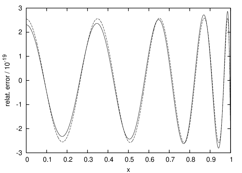
The actual relative error of this approximation is shown in Fig. 1 as a continuous line, with a maximum of $2.9\cdot 10^{-19}$ . The dashed line with a relative error of $2.6\cdot 10^{-19}$ in comparison results from further minimax optimization with coefficients shown in the next table:

Refer to caption — Figure 1. The relative error $R(x)$ to $f(x)=\sin(\pi x/2)/x$ for both tabulated parameter sets of $\sum_{n=0,2,\ldots}^{16}b_{n}T_{n}(x)$ of Example 5.9.

$n$	$b_{n}$	$d_{n}$
0	1.2762789624022658802075437	1.5707963267948966188314659
2	-0.2852615691810360095705230	- 0.6459640975062461915471363
4	0.9118016006651802497528156 $\cdot 10^{-2}$	0.7969262624616544421893744 $\cdot 10^{-1}$
6	-0.1365875135419666726405733 $\cdot 10^{-3}$	-0.4681754135302704719117724 $\cdot 10^{-2}$
8	0.1184961857661689920542732 $\cdot 10^{-5}$	0.1604411847070460989830944 $\cdot 10^{-3}$
10	-0.6702791603827612608171959 $\cdot 10^{-8}$	-0.3598843007652658555526627 $\cdot 10^{-5}$
12	0.2667278599019855592489579 $\cdot 10^{-10}$	0.5692134921914455833455723 $\cdot 10^{-7}$
14	-0.7872921659616258733890169 $\cdot 10^{-13}$	-0.6684324580312975131354658 $\cdot 10^{-9}$
16	0.1791589025538146793760922 $\cdot 10^{-15}$	0.5870678918883399413795788 $\cdot 10^{-11}$

Example 5.10.

As an example for (4.18), consider $\exp(x)=\mathop{{\sum}^{\prime}}_{n=0}^{\infty}f_{n}T^{*}_{n}(x)$ over $0\leq x\leq 1$ [1, (4.2.48)][5, 19]. The $f_{n}$ are represented via [1, (9.6.26] through modified Bessel Functions $I_{n}$ ,

(5.16)

f_{n}=2\sqrt{e}I_{n}(1/2);\quad f_{n+1}=-4nf_{n}+f_{n-1},

$n$	$f_{n}$
0	3.506775308754180791443893
1	0.8503916537808109665352350
2	0.1052086936309369253029528
3	0.008722104733315564111612874
4	0.0005434368311501559635982758
5	0.00002711543491306869404046064

Truncation of the Chebyshev series for $f(x)$ after $k=3$ yields an estimated maximum absolute error of $\sum_{n=k+1}^{N}|f_{n}|\approx 5.7\cdot 10^{-4}$ evaluated at $N=9$ . The relative error of the same polynomial is $\mathop{{\sum}^{\prime}}_{n=0}^{N}|\hat{a}_{n}|-1\approx 5.1\cdot 10^{-4}$ . After four Newton iterations, this value drops to $4.0\cdot 10^{-4}$ with coefficients given in the following table:

$n$	$b_{n}$
0	1.753387654377090395721946
1	0.8503902561425088936327743
2	0.1051918520893768747555014
3	0.008587089960927766771654559

If we proceed to $k=12$ at $N=36$ , the estimated maximum relative error becomes $6.1\cdot 10^{-18}$ with the following coefficients:

$n$	$b_{n}$	$d_{n}$
0	1.7533876543770903957219464	1.0000000000000000060373678
1	0.8503916537808109665352350	0.9999999999999978889799411
2	0.1052086936309369253029528	0.5000000000001216148194572
3	0.8722104733315564111612874 $\cdot 10^{-2}$	0.1666666666639271874501180
4	0.5434368311501559635982758 $\cdot 10^{-3}$	0.4166666669859109153386033 $\cdot 10^{-1}$
5	0.2711543491306869404045765 $\cdot 10^{-4}$	0.8333333112815145481691497 $\cdot 10^{-2}$
6	0.1128132888782082788967416 $\cdot 10^{-5}$	0.1388889862738933258163839 $\cdot 10^{-2}$
7	0.4024558229870710027066467 $\cdot 10^{-7}$	0.1984098287973665146421103 $\cdot 10^{-3}$
8	0.1256584418283842256517024 $\cdot 10^{-8}$	0.2480734627092463176804164 $\cdot 10^{-4}$
9	0.3488091362080888722258141 $\cdot 10^{-10}$	0.2747848541489261879291146 $\cdot 10^{-5}$
10	0.8715278679388174731063544 $\cdot 10^{-12}$	0.2827881515524984459349078 $\cdot 10^{-6}$
11	0.1979783472020383084286900 $\cdot 10^{-13}$	0.2086709669366350082217004 $\cdot 10^{-7}$
12	0.4103178180353125619414324 $\cdot 10^{-15}$	0.3441995330913567239602395 $\cdot 10^{-8}$

Equilibration of the local extrema with the following coefficients reduces this error to $5.0\cdot 10^{-18}$ :

$n$	$b_{n}$	$d_{n}$
0	1.7533876543770903961757996	1.0000000000000000049913878
1	0.8503916537808109674449984	0.9999999999999982006556032
2	0.1052086936309369262175803	0.5000000000001063630793784
3	0.8722104733315565035195027 $\cdot 10^{-2}$	0.1666666666642173677701902
4	0.5434368311501568988037582 $\cdot 10^{-3}$	0.4166666669575619866774579 $\cdot 10^{-1}$
5	0.2711543491306964588901369 $\cdot 10^{-4}$	0.8333333129071360606767972 $\cdot 10^{-2}$
6	0.1128132888783054546376918 $\cdot 10^{-5}$	0.1388889803905621871712292 $\cdot 10^{-2}$
7	0.4024558229970401854905218 $\cdot 10^{-7}$	0.1984099684263107292542263 $\cdot 10^{-3}$
8	0.1256584419307581158766302 $\cdot 10^{-8}$	0.2480712594971168345247335 $\cdot 10^{-4}$
9	0.3488091466142981067488685 $\cdot 10^{-10}$	0.2748077480706561519632930 $\cdot 10^{-5}$
10	0.8715288225355426665019433 $\cdot 10^{-12}$	0.2826376902452534679601836 $\cdot 10^{-6}$
11	0.1979820112783685973416909 $\cdot 10^{-13}$	0.2092376435267840500466468 $\cdot 10^{-7}$
12	0.4092071997914099904014169 $\cdot 10^{-15}$	0.3432678789827820176761249 $\cdot 10^{-8}$

6. Summary

Besides some generic algorithms to compute the Chebyshev series of inverse polynomials, there are two specific aspects that facilitate this task: (i) the expansion coefficients can be derived from the partial fractions of the inverse polynomial. (ii) Expansion coefficients with indices larger than the polynomial degree are recursively linked to those of lower order. (iii) An algorithm has been presented which derives a polynomial of a given degree such that the first terms of the Chebyshev expansion of the relative error of a given function represented by this polynomial vanish.

Appendix A Chebyshev Series of $\ln(1+x)$

The integral representation

(A.1)

\ln(1+x)=\int\frac{dx}{1+x}

and term-by-term integration of (2.10) on the r.h.s. with (2.9) yield that the Chebyshev coefficients of

(A.2)

f(x)=\ln(1+x)\equiv\mathop{{\sum}^{\prime}}_{n=0}^{\infty}f_{n}T_{n}^{*}(x)\,\quad 0\leq x\leq 1,

obey

(A.3)

2nf_{n}=a_{n+1,1}(-3)-a_{n-1,1}(-3),\quad n\geq 1,

explicitly [13, p. 88][14]

(A.4)

f_{n}=\frac{2(-)^{n+1}}{n(3+2\sqrt{2})^{n}},\quad n\geq 1

from (2.11), as tabulated in [1, 4.1.45]. The missing $f_{0}$ is

(A.5)

f_{0}=\frac{2}{\pi}\int_{0}^{1}\frac{\ln(1+x)}{\sqrt{x(1-x)}}dx=2\ln\frac{3+2\sqrt{2}}{4},

because insertion of $x=1$ in (A.2) yields

(A.6)

f_{0}=2\left(f(1)-\sum_{n=1}^{\infty}f_{n}\right)

and $f(1)=\ln 2$ and $\sum_{n=1}^{\infty}f_{n}=2\ln(1+\frac{1}{3+2\sqrt{2}})$ via [1, 4.1.24].

Appendix B Chebyshev Series of $\arctan x$

Integrating (2.7) over $x$ with

(B.1)

\int\frac{1}{1+x^{2}}dx=\arctan x

and (1.5) we get [13, p. 89][14]

(B.2)

\arctan x=2\sum_{j=1,3,5,7,\ldots}\frac{(-)^{\lfloor j/2\rfloor}}{j(1+\sqrt{2})^{j}}T_{j}(x),\quad-1\leq x\leq 1,

in particular at $x=1$

(B.3)

\frac{\pi}{8}=\sum_{j=1,3,5,7,\ldots}\frac{(-)^{\lfloor j/2\rfloor}}{j(1+\sqrt{2})^{j}}.

From (B.2) and (1.15), the coefficients of

(B.4)

\frac{\arctan x}{x}\equiv\mathop{{\sum}^{\prime}}_{n=0,2,4,6,\ldots}g_{n}T_{n}(x)

as listed in [1, (4.4.50)][5] follow recursively, where $g_{0}=2\ln(1+\sqrt{2})$ is obtained via [15, 4.531.12].

Appendix C Chebyshev Series of $\arcsin x$

The series of $\arcsin x=\sum_{n=1,3,5,\ldots}^{\infty}g_{n}T_{n}(x)$ starts with $g_{1}=4/\pi$ . A combination of [1, (4.4.58)], (1.4), (1.5) and [28, (3.4.1d)]

(C.1)

\sqrt{1-x^{2}}=\frac{4}{\pi}\mathop{{\sum}^{\prime}}_{\genfrac{}{}{0.0pt}{}{n=0}{n\, \text{even}}}^{\infty}\frac{1}{1-n^{2}}T_{n}(x)

yields

(C.2)

(n+1)g_{n+1}+(n-1)g_{n-1}=\frac{8}{\pi}\frac{n}{n^{2}-1},\quad n=2,4,6,.\dots

in this case, which can be unwound as $g_{n}=4/(\pi n^{2})$ . To find a formulation with controlled relative error, we would switch to $h(x)=(\arcsin x)/x=\mathop{{\sum}^{\prime}}_{n=0}^{\infty}h_{n}T_{n}(x)$ to remove the zero in the spirit of example 5.5. With (1.15), the expansion coefficients are

(C.3)		$\displaystyle h_{0}$	$\displaystyle=$	$\displaystyle 8\beta(2)/\pi,$
(C.4)		$\displaystyle h_{n+2}$	$\displaystyle=$	$\displaystyle-h_{n}+\frac{8}{\pi(n+1)^{2}},$

where $\beta(2)\approx 0.915965594177219015054603515$ is Catalan’s constant [1, Tab 23.3][15, 0.234.3].

Appendix D Chebyshev Series of $\arcsin(x/\surd 2)$

The coefficients of

(D.1)

\arcsin(x/\sqrt{2})=\sum_{n=1,3,5,\ldots}^{\infty}k_{n}T_{n}(x)

are found by partial integration of $\int\arcsin([\cos\theta]/\surd 2)\cos(n\theta)d\theta$

(D.2)

k_{n}=\frac{1}{n\pi}\left[\int_{0}^{\pi}\frac{\cos[(n-1)\theta]}{\sqrt{2-\cos^{2}\theta}}d\theta-\int_{0}^{\pi}\frac{\cos[(n+1)\theta]}{\sqrt{2-\cos^{2}\theta}}d\theta\right],\quad n\,\text{odd}

where

(D.3)

\int_{0}^{\pi}\frac{\cos(2m\theta)}{\sqrt{2-\cos^{2}\theta}}d\theta=G_{2m}=\left\{\begin{array}[]{ll}\sqrt{2}F(\frac{1}{\sqrt{2}})\approx 2.6220575542921198104648395899,&m=0,\\ \sqrt{2}[3F(\frac{1}{\sqrt{2}})-4E(\frac{1}{\sqrt{2}})]\approx 0.22577708482093539558499460534,&m=1,\\ \end{array}\right.

are Complete Elliptic Integrals. To find a recurrence for these

(D.4)

G_{s}\equiv\int_{-1}^{1}\frac{T_{s}(x)}{\sqrt{(2-x^{2})(1-x^{2})}}dx,

we apply the method of [1, (17.1.4)] to the quartic $y^{2}\equiv(2-x^{2})(1-x^{2})$ , with $d(yT_{s}(x))/dx=y(dT_{s}(x)/dx)+T_{s}\frac{1}{2y}(T_{3}(x)-3T_{1}(x))$ , insert (1.6) for the derivative on the r.h.s, replace the first $y$ on the r.h.s. by $y^{2}/y=(T_{4}/8-T_{2}+7/8)/y$ , expand all products with (1.4), and finally insert the upper limit $x=1$ where $y(x)T_{s}(x)=0$ :

(D.5)

G_{s+3}+G_{|s-3|}-3(G_{s+1}+G_{|s-1|})+\frac{s}{2}\mathop{{\sum}^{\prime}}_{\genfrac{}{}{0.0pt}{}{l=0}{l-s\, \text{odd}}}^{s-1}\left[G_{l+4}+G_{|l-4|}-8(G_{l+2}+G_{|l-2|})+14G_{l}\right]=0.

Inserting $s=1,3,5$ and 7, for example, yields

(D.6)	$\displaystyle 3G_{4}-12G_{2}+G_{0}$	$\displaystyle=$	$\displaystyle 0,$
(D.7)	$\displaystyle 5G_{6}-27G_{4}+15G_{2}-G_{0}$	$\displaystyle=$	$\displaystyle 0,$
(D.8)	$\displaystyle 7G_{8}-41G_{6}+29G_{4}-3G_{2}$	$\displaystyle=$	$\displaystyle 0,$
(D.9)	$\displaystyle 9G_{10}-55G_{8}+43G_{6}-5G_{4}$	$\displaystyle=$	$\displaystyle 0,$

and generates $k_{1}$ to $k_{9}$ in (D.2) from $G_{0}$ and $G_{2}$ shown in (D.3). A slowly converging series expansion is also known [4, 806.01]. With (1.15) we find the coefficients $f_{n}=2k_{n-1}-f_{n-2}$ for

(D.10)

\frac{1}{x}\arcsin\frac{x}{\sqrt{2}}=\mathop{{\sum}^{\prime}}_{n=0,2,4,\ldots}^{\infty}f_{n}T_{n}(x),\quad-1\leq x\leq 1,

starting at

(D.11)		$\displaystyle f_{0}$	$\displaystyle=$	$\displaystyle\frac{4}{\pi}\int_{0}^{1}\frac{\arcsin\frac{x}{\sqrt{2}}}{x\sqrt{1-x^{2}}}dx=\sqrt{2}\sum_{l=0}^{\infty}\frac{[(2l-1)!!]^{2}}{2^{l}(2l+1)[(2l)!!]^{2}}$
(D.11)			$\displaystyle=$	$\displaystyle\frac{\pi}{2}-\frac{4}{\pi}\sum_{q=1}^{\infty}\frac{1}{4q-1}\left[G_{4q-2}-G_{4q}\right]\approx 1.4866664932871034689603296833.$

The four coefficients $\alpha_{i}$ that span

(D.12)

k_{n-1}=\frac{\surd 2}{\pi}\left[\alpha_{1}K(\frac{1}{\sqrt{2}})+\alpha_{2}E(\frac{1}{\sqrt{2}})\right],\quad f_{n}=\frac{\surd 2}{\pi}\left[\alpha_{3}K(\frac{1}{\sqrt{2}})+\alpha_{4}E(\frac{1}{\sqrt{2}})\right]+(-)^{[n/2]}f_{0},

start as follows:

$n$	$\alpha_{1}$	$\alpha_{2}$	$\alpha_{3}$	$\alpha_{4}$
2	-2	4	-4	8
4	-26/9	4	-16/9	0
6	-638/75	292/25	-3428/225	584/25
8	-22702/735	212/5	-513088/11025	1536/25
10	-23722/189	4652/27	-6763436/33075	191128/675
12	-463174/847	2252/3	-3558618544/4002075	822272/675
14	-162508858/65065	8691484/2535	-2777152623884/676350675	643269592/114075

Because $T_{2j}(x)=T_{j}^{*}(x^{2})$ , the following numbers coincide with [1, (4.4.51)] up to a factor $\surd 2$ :

$n$	$f_{n}$	$n$	$f_{n}$
2	0.3885303371652290716432228 $\cdot 10^{-1}$
4	0.2885441422084471126676825 $\cdot 10^{-2}$	6	0.2884218334475536563483289 $\cdot 10^{-3}$
8	0.3322367192785279209254231 $\cdot 10^{-4}$	10	0.4158477878052832866177270 $\cdot 10^{-5}$
12	0.5496504525974164467345493 $\cdot 10^{-6}$	14	0.7550078449371525934251585 $\cdot 10^{-7}$
16	0.1067193805629843129424091 $\cdot 10^{-7}$	18	0.1542180379281470021561106 $\cdot 10^{-8}$
20	0.2268114598545151963877153 $\cdot 10^{-9}$	22	0.3383885639342775871004709 $\cdot 10^{-10}$
24	0.5108937524377197224216916 $\cdot 10^{-11}$	26	0.7791139213632464421446539 $\cdot 10^{-12}$
28	0.1198378589352895337866326 $\cdot 10^{-12}$	30	0.1856972621821342234640637 $\cdot 10^{-13}$
32	0.2896189154386304361020997 $\cdot 10^{-14}$	34	0.4542792886328823081478511 $\cdot 10^{-15}$
36	0.7161678029265506176831289 $\cdot 10^{-16}$	38	0.1134144256904559996509711 $\cdot 10^{-16}$

Appendix E Chebyshev Series of $\psi(x+2)$

An expansion of the Digamma function [34] is [1, (6.3.16)]

(E.1)

\psi(2+x)=1-\gamma+x\sum_{k=2}^{\infty}\frac{1}{k(x+k)},

where $\gamma\approx 0.5772$ is Euler’s constant. Employing $a_{n,1}(-k)$ of (2.4),

(E.2)

\frac{1}{x+k}=-\frac{1}{-k-x}=\frac{2}{\sqrt{k^{2}-1}}\mathop{{\sum}^{\prime}}_{n=0}^{\infty}\frac{(-)^{n}}{(k+\sqrt{k^{2}-1})^{n}}T_{n}(x),\quad-1\leq x\leq 1,

(E.3)

\psi(2+x)=1-\gamma+2x\sum_{k=2}^{\infty}\frac{1}{k\sqrt{k^{2}-1}}\mathop{{\sum}^{\prime}}_{n=0}^{\infty}\frac{(-)^{n}}{(k+\sqrt{k^{2}-1})^{n}}T_{n}(x).

The auxiliary definition

(E.4)

K_{n}\equiv\sum_{k=2}^{\infty}\frac{1}{k\sqrt{k^{2}-1}(k+\sqrt{k^{2}-1})^{n}},\quad n=0,1,2,\ldots

turns (E.3) with the aid of (1.4) into

(E.5)

\psi(x+2)=(1-\gamma-K_{1})T_{0}(x)-\sum_{n=1}^{\infty}(-)^{n}(K_{n-1}+K_{n+1})T_{n}(x),\quad-1\leq x\leq 1,

where

(E.6)

K_{n}+K_{n+2}=2\sum_{k=2}^{\infty}\frac{1}{\sqrt{k^{2}-1}(k+\sqrt{k^{2}-1})^{n+1}},\quad n=0,1,2,\ldots

Alternatives to the slowly converging original series (E.4) at small $n$ are obtained in terms of the Riemann Zeta function $\zeta$ after reducing the fraction in (E.4) and/or (E.6) by $k-\sqrt{k^{2}-1}$ ,

(E.7)	$\displaystyle K_{0}$	$\displaystyle=$	$\displaystyle\sum_{k=2}^{\infty}\frac{1}{k^{2}}\left(1-\frac{1}{k^{2}}\right)^{-1/2}=\sum_{l=0}^{\infty}(-)^{l}\genfrac{(}{)}{0.0pt}{}{-1/2}{l}[\zeta(2l+2)-1],$
(E.8)	$\displaystyle K_{1}$	$\displaystyle=$	$\displaystyle\sum_{k=2}^{\infty}\frac{k-\sqrt{k^{2}-1}}{k\sqrt{k^{2}-1}}=\sum_{l=1}^{\infty}(-)^{l}\genfrac{(}{)}{0.0pt}{}{-1/2}{l}[\zeta(2l+1)-1],$
(E.9)	$\displaystyle K_{0}+K_{2}$	$\displaystyle=$	$\displaystyle 2\sum_{l=1}^{\infty}(-)^{l}\genfrac{(}{)}{0.0pt}{}{-1/2}{l}[\zeta(2l)-1],$
(E.10)	$\displaystyle K_{1}+K_{3}$	$\displaystyle=$	$\displaystyle 2\sum_{l=2}^{\infty}(-)^{l}\left(\genfrac{(}{)}{0.0pt}{}{-1/2}{l}+\genfrac{(}{)}{0.0pt}{}{1/2}{l}\right)[\zeta(2l-1)-1],$
(E.11)	$\displaystyle K_{n}+K_{n+2}$	$\displaystyle=$	$\displaystyle 2\sum_{l=[(n+3)/2]}^{\infty}(-)^{l}[\zeta(2l-n)-1]\sum_{s=0}^{n+1}\genfrac{(}{)}{0.0pt}{}{n+1}{s}\genfrac{(}{)}{0.0pt}{}{(s-1)/2}{l}.$

$n$	$K_{n}$	$n$	$K_{n}$
0	0.6942240199692270653811973	1	0.1181923495113155830503315
2	0.2615575442260127035429158 $\cdot 10^{-1}$	3	0.6357242927298094244957032 $\cdot 10^{-2}$
4	0.1613702909326556648518537 $\cdot 10^{-2}$	5	0.4189942166841513997803225 $\cdot 10^{-3}$
6	0.1101726048982138724638504 $\cdot 10^{-3}$	7	0.2918277395837793537278094 $\cdot 10^{-4}$
8	0.7763995103341854698876680 $\cdot 10^{-5}$	9	0.2071120322602199079344235 $\cdot 10^{-5}$
10	0.5534045978754736410165904 $\cdot 10^{-6}$	11	0.1480224417758054637706871 $\cdot 10^{-6}$
12	0.3961806941781982189370558 $\cdot 10^{-7}$	13	0.1060807013890109056491206 $\cdot 10^{-7}$
14	0.2841134565373781348071928 $\cdot 10^{-8}$	15	0.7610594780500236739360477 $\cdot 10^{-9}$
16	0.2038876075855356359426642 $\cdot 10^{-9}$	17	0.5462507275750785409310247 $\cdot 10^{-10}$
18	0.1463563991421891531670298 $\cdot 10^{-10}$	19	0.3921418684181661587649434 $\cdot 10^{-11}$
20	0.1050708536652289553110610 $\cdot 10^{-11}$	21	0.2815309431326615497301838 $\cdot 10^{-12}$
22	0.7543503527420115661214215 $\cdot 10^{-13}$	23	0.2021259323594124792356794 $\cdot 10^{-13}$
24	0.5415919982188370035264436 $\cdot 10^{-14}$	25	0.1451186573479985220441655 $\cdot 10^{-14}$
26	0.3888434449455691142432431 $\cdot 10^{-15}$	27	0.1041901454404881356692972 $\cdot 10^{-15}$
28	0.2791764103483896329393674 $\cdot 10^{-16}$

As a by-product, insertion of $x=\pm 1$ in (E.3) with $\psi(1)=-\gamma$ shows

(E.12)		$\displaystyle\sum_{k=2}^{\infty}\frac{1}{k\sqrt{k^{2}-1}}\frac{k-1+\sqrt{k^{2}-1}}{k+1+\sqrt{k^{2}-1}}$	$\displaystyle=$	$\displaystyle\frac{1}{2},$
(E.13)		$\displaystyle\sum_{k=2}^{\infty}\frac{1}{k\sqrt{k^{2}-1}}\frac{k+1+\sqrt{k^{2}-1}}{k-1+\sqrt{k^{2}-1}}$	$\displaystyle=$	$\displaystyle 1.$

Linear combinations of these two equations are

(E.14)		$\displaystyle\sum_{k=2}^{\infty}\frac{(k-3)(k+\sqrt{k^{2}-1})}{k\sqrt{k^{2}-1}[(k+\sqrt{k^{2}-1})^{2}-1]}$	$\displaystyle=$	$\displaystyle 0,$
(E.15)		$\displaystyle\sum_{k=2}^{\infty}\frac{k+\sqrt{k^{2}-1}}{k\sqrt{k^{2}-1}[(k+\sqrt{k^{2}-1})^{2}-1]}$	$\displaystyle=$	$\displaystyle\frac{1}{8},$

and these two can be combined to

(E.16)

\sum_{k=2}^{\infty}\frac{k+\sqrt{k^{2}-1}}{\sqrt{k^{2}-1}[(k+\sqrt{k^{2}-1})^{2}-1]}=\frac{3}{8}.

References

[1] Milton Abramowitz and Irene A. Stegun (eds.), Handbook of mathematical functions, 9th ed., Dover Publications, New York, 1972.
[2] R. Barrio, Algorithms for the integration and derivation of Chebyshev series, Appl. Math. Comp. 150 (2004), 707–717. MR MR2039669 (2005a:65019)
[3] Yu. G. Bulychev and E. Yu. Bulycheva, Some new properties of the Chebychev polynomials and their use in analysis and design of dynamic systems, Autom. Remote Control 64 (2003), no. 4, 554–563.
[4] Paul F. Byrd and Morris D. Friedman, Handbook of elliptical integrals for engineers and physicists, 2nd ed., Die Grundlehren der mathematischen Wissenschaften in Einzeldarstellungen, vol. LXVII, Springer, Berlin, Göttingen, 1971. MR MR0277773 (43 #3506)
[5] C. W. Clenshaw, Polynomial approximations to elementary functions, Math. Tabl. Aids Comput. 8 (1954), no. 47, 143–147. MR 16,128f
[6] C. W. Clenshaw and A. R. Curtis, A method for numerical integration on an automatic computer, Numer. Math. 2 (1960), 197–205. MR 22 #8659
[7] W. J. Cody, A survey of practical rational and polynomial approximation of functions, SIAM Rev. 12 (1970), no. 3, 400–423. MR 42 #2627
[8] David Elliott, The evaluation and estimation of the coefficients in the Chebyshev series expansion of a function, Math. Comp. 18 (1964), no. 86, 274–284.
[9] David Elliott and George Szekeres, Some estimates of the coefficients in the Chebyshev series expanion of a function, Math. Comp. 19 (1965), no. 89, 25–32.
[10] Henry E. Fettis, Numerical calculation of certain definite integrals by Poisson’s summation formula, Math. Tabl. Aids Comput. 9 (1955), no. 51, 85–92. MR 17,302f
[11] Jerry L. Fields and Jet Wimp, Expansions of hypergeometric functions in series of other hypergeometric functions, Math. Comp. 15 (1961), no. 76, 390–395, In the second line of (2.10), the fraction bar in the argument of ${}_{1}F_{1}$ should be removed. MR 23 #A3289
[12] Lloyd D. Fosdick, A special case of the Filon quadrature formula, Math. Comp. 22 (1968), no. 101, 77–81. MR 37 #1078
[13] Leslie Fox and Ian Bax Parker, Chebyshev polynomials in numerical analysis, Oxford mathematical handbooks, Oxford University Press, Oxford, 1968.
[14] W. Fraser, A survey of methods of computing minimax and near-minimax polynomial approximations for functions of a single independent variable, J. ACM 12 (1965), no. 3, 295–314.
[15] I. Gradstein and I. Ryshik, Summen-, Produkt- und Integraltafeln, 1st ed., Harri Deutsch, Thun, 1981. MR 83i:00012
[16] Takemitsu Hasegawa and Tatsuo Torii, An automatic quadrature for Cauchy principal value integrals, Math. Comp. 56 (1991), no. 194, 741–754. MR 91j:65051
[17] Takemitsu Hasegawa, Tatsuo Torii, and Ichizo Ninomiya, Generalized Chebyshev interpolation and its application to automatic quadrature, Math. Comp. 41 (1983), no. 164, 537–553. MR 84m:65037
[18] A. P. Holub, Pade-Chebyshev approximants for one class of functions, Ukr. Math. J. 54 (2002), no. 1, 15–19.
[19] H. G. Khajah and E. L. Ortiz, Ultra-high precision computations, Comp. Math. Applic. 27 (1994), no. 7, 41–57. MR MR1265397
[20] M. Kzaz and M. Prévost, Convergence acceleration of Gauss-Chebyshev quadrature formulae, Numer. Algorithms 34 (2003), no. 2–4, 379–391. MR 2 043 910
[21] J. C. Mason, The minimality properties of Chebyshev polynomials and their lacunary series, Numer. Algorithms 38 (2005), no. 1, 61–78.
[22] J. C. Mason and E. Venturino, A Chebyshev polynomial method for line integrals with singularities, Adv. Comput. Math. 10 (1999), 187–208. MR 2000a:65029
[23] F. D. Murnaghan and J. W. Wrench Jr., The determination of the Chebyshev approximating polynomial for a differentiable function, Math. Tabl. Aids Comput. 13 (1959), no. 67, 185–193. MR 21 #4526
[24] Johannes C. C. Nitsche, Über die Abhängigkeit der Tschebyscheffschen Approximierenden einer differenzierbaren Funktion vom Intervall, Numer. Math. 4 (1962), 262–276. MR 26 #6657
[25] F. Pérez-Acosta and P. González Vera, A note on quadrature formulas for the Chebyshev weight function of the First Kind, Appl. Math. Lett. 7 (1994), no. 3, 97–100. MR 1 350 384
[26] Abedallah Rababah, Transformaion of Chebyshev-Bernstein polynomial basis, Comput. Meth. Appl. Math. 3 (2003), no. 4, 608–622.
[27] T. J. Rivlin, Polynomials of best uniform approximation to certain rational functions, Numer. Math. 4 (1962), 345–349. MR 26 #6653
[28] Theodore J. Rivlin, The Chebyshev Polynomials, Pure and Applied Mathematics, John Wiley, New York, London, 1974. MR MR0450850 (56 #9142)
[29] Jun Sawada and Ruben Gamboa, Mechanical verification of a square root algorithm using taylor’s theorem, Formal Methods in Computer-Aided Design: 4th International Conference, FMCAD 2002, Portland, OR, USA, November 6–8, 2002 (M. D. Aagaard and J. W. O’Leary, eds.), Lecture Notes in Computer Science, vol. 2517, Springer, Berlin, Heidelberg, 2003, pp. 274–291.
[30] J. L. Schonfelder, Very high accuracy Chebyshev expansions for the basic trigonometric functions, Math. Comp. 34 (1980), no. 149, 237–244. MR 81f:65016
[31] R. E. Scraton, A comparison of some Taylor and Chebyshev series, Math. Comput. 50 (1988), no. 181, 207–213.
[32] Rahul Sen, Closed-form expressions for certain induction integrals involving Jacobi and Chebyshev polynomials, J. Comput. Phys. 156 (1999), no. 2, 393–398. MR 1 727 338
[33] H. V. Smith, Some error expansions for certain Gaussian quadrature rules, J. Comput. Appl. Math. 155 (2003), no. 2, 331–337. MR 2004e:65025
[34] John L. Spouge, Computation of the gamma, digamma and trigamma functions, SIAM J. Numer. Anal. 31 (1994), no. 3, 931–944.
[35] Balth van der Pol and Th. J. Weijers, Tchebyscheff polynomials and their relation to circular functions, Besselfunctions and Lissajous-figures, Physica 1 (1934), 78–96.
[36] L. Veidinger, On the numerical determination of the best approximations in the Chebyshev sense, Numer. Math. 2 (1960), 99–105. MR 25 #3316

Chebyshev Series Expansion of Inverse Polynomials

Abstract.

Key words and phrases:

2000 Mathematics Subject Classification

1. Introduction and Scope

Remark 1.1.

Remark 1.2.

2. The Case of Known Partial Fractions

Example 2.1.

Remark 2.2.

Example 2.3.

Remark 2.4.

Example 2.5.

Example 2.6.

Remark 2.7.

Remark 2.8.

3. Recurrence of Expansion Coefficients

Proof.

Example 3.1.

4. Approximation by the Truncated Chebyshev Series

Example 4.1.

Remark 4.2.

Example 4.3.

Remark 4.4.

5. Chebyshev Approximation for the Relative Error

Remark 5.1.

Remark 5.2.

Example 5.3.

Example 5.4.

Example 5.5.

Example 5.6.

Example 5.7.

Example 5.8.

Example 5.9.

Example 5.10.

6. Summary

Appendix A Chebyshev Series of ln⁡(1+x)\ln(1+x)

Appendix B Chebyshev Series of arctan⁡x\arctan x

Appendix C Chebyshev Series of arcsin⁡x\arcsin x

Appendix D Chebyshev Series of arcsin⁡(x/2)\arcsin(x/\surd 2)

Appendix E Chebyshev Series of ψ⁡(x+2)\psi(x+2)

References

Appendix A Chebyshev Series of $\ln(1+x)$

Appendix B Chebyshev Series of $\arctan x$

Appendix C Chebyshev Series of $\arcsin x$

Appendix D Chebyshev Series of $\arcsin(x/\surd 2)$

Appendix E Chebyshev Series of $\psi(x+2)$