On the additivity of knot width

In [G] Gabai associated to a knot in $3$–space an even number called its width (see Definition 2 below for the precise definition). Width can be viewed as a generalization of bridge number, an invariant first studied by Schubert [S]. Schubert’s remarkable discovery was that, for $b(K)$ the bridge number of $K\subset S^{3}$, it is always true that

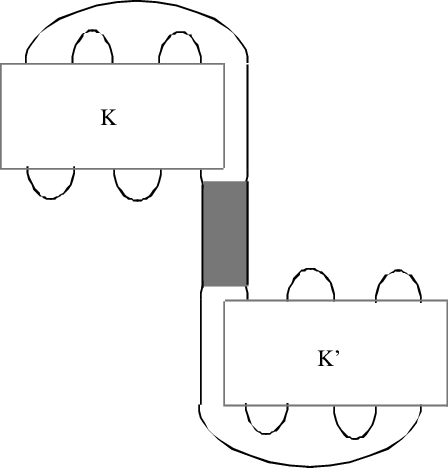
An alternative formulation of what Schubert showed is this: one way of putting the knot sum $K\#K^{\prime}$ into minimal bridge position is to put both $K,K^{\prime}$ into minimal bridge position, then place them vertically adjacent in $S^{3}$. Then create their knot sum via a vertical band (see Figure 1).

Because width generalizes the notion of bridge number, it is natural to hope that a similar equality is true for width. Just as the construction described above and shown in Figure 1 makes it obvious that

(Schubert’s deep contribution is the proof of the reverse inequality, see [Sch]), it also shows that knot width $w$ satisfies the inequality

That is, the resulting presentation of $K\#K^{\prime}$ has width precisely equal to $w(K)+w(K^{\prime})-2$. The inequality reflects uncertainty over whether this presentation is of minimal width (that is, thin) among all possible presentations for $K\#K^{\prime}$. This suggests the following

Beyond the analogy with bridge number, and the ease of the inequality in one direction, there are two pieces of evidence for Conjecture 1. One piece of evidence is the proof in [RS] that the conjecture is true for knots that are small, that is, knots which have no closed essential surfaces in their complements. A second but weaker piece of evidence is the proof in [ScSc] that in any case,

This shows that at least some inequality in the reverse direction is true.

The aim here is to present an example of a knot (actually a family of knots) $K_{1}$ which appears to have the property that

whenever $K_{2}$ is a $2$–bridge knot. Since the width of a $2$–bridge knot is $8$, this would be a counterexample to Conjecture 1. Although we are not able to prove this equality, the construction of $K_{1}$ is so flexible that the example does seem to undercut any hope that the conjecture is true. Only the absence so far of a good method to prove that our presentation of the knot (family) $K_{1}$ is the presentation of least width stands in the way of a complete proof that at least some of these knots are counterexamples to Conjecture 1.

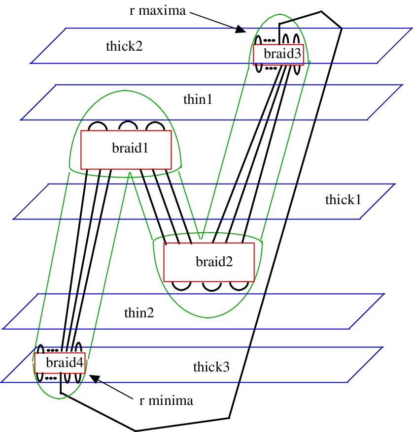
The example $K_{1}$ is shown in Figure 2. It is actually a family of examples, because specific braids inside of boxes are not specified; the point will be that, in search of an example, the number of critical points $r$ can be made arbitrarily high and the braids themselves be made arbitrarily complicated.

Figure 3 shows an imbedding of $K_{1}\#(\rm{trefoil})$ into $S^{3}$; a decomposing sphere is shown in the figure. Note that the width of the presentations of $K_{1}$ and $K_{1}\#(\rm{trefoil})$ with respect to the vertical height function are the same, since there is an obvious level-preserving reimbedding of one to the other. (The construction of $K_{1}$ was inspired by the extensive use of level-preserving reimbeddings in [ScSc].) Moreover, the only property of the trefoil knot that is used in the level-preserving reimbedding is the fact that it is $2$–bridge — any other $2$–bridge knot would do.

If we knew that the given presentation of the knot $K_{1}$ is thin (that is, of minimal width) we would be done. We do not yet know a full proof of this, but cite two pieces of evidence:

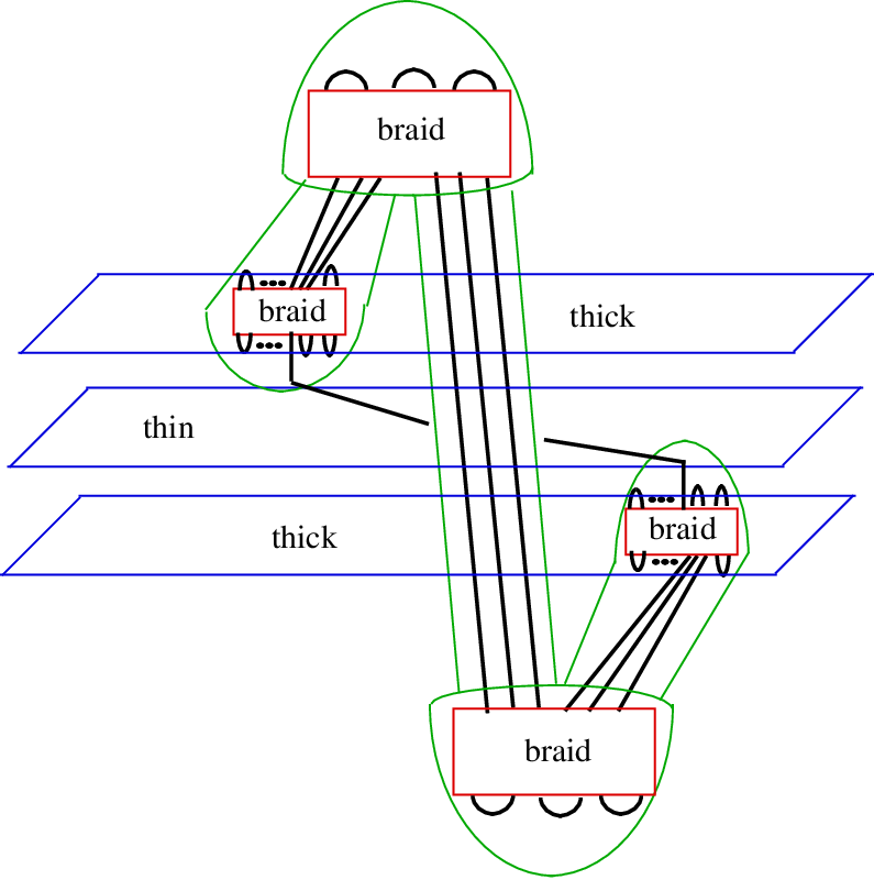
First of all, the braids in the four braid boxes of Figure 2 may be made very complicated so that the number of critical points of a plane sweeping across the boxes in any direction except the vertical will have a large number of critical points and arbitrarily high width. Although this does not obviously rule out the possibility of more complicated sweep-outs, it seems very likely that with sufficiently complicated braids in place a sweep-out can only be thin for the whole knot if the sweep-out passes through these braid-boxes vertically, that is as horizontal planes, just as in the given presentation. (This is a stronger requirement than merely ensuring that the tangles within the braid boxes are thin.) Once this is ensured, the order in which the sweep-out passes through each tangle could be compared to the given order; alternative orders, such as the order shown in Figure 4, will give rise to greater width (see calculation below) as long as $r\geq 4$.

This second but indirect bit of evidence that $K_{1}$ is thin is this: According to Schubert’s theorem, there is a presentation of $K_{1}$ with lower bridge number than that of $K_{1}\#(\rm{trefoil})$ shown in Figure 3. But the Figure 3 presentation has the same bridge number as the presentation of $K_{1}$ shown in Figure 2. Given that width is a generalization of bridge number, we ought to check that the presentation that lowers bridge number from that in Figure 2 does not also lower width. Figure 4 shows a presentation of $K_{1}$ that has lower bridge number than the original presentation, shown in Figure 2. But in fact the presentation of $K_{1}$ in Figure 4 is not as thin as that in Figure 2.

To explicitly compare the widths of the two presentations, recall the definitions (see [ScSc]):

The key operational feature of width is that it is reduced if a minimum is pushed up above a maximum whereas switching the levels of two adjacent minima or two adjacent maxima has no effect.

There is an easier way to calculate width. For the levels $r_{i}$ described above, call $r_{i}$ a thin level of $K$ (and the sphere $S^{r_{i}}$ a thin sphere for $K$) with respect to $p$ if $c_{i}$ is a maximum value for $p|K$ and $c_{i+1}$ is a minimum value for $p|K$. Dually $r_{i}$ is a thick level of $K$ (and the sphere $S^{r_{i}}$ a thick sphere for $K$) with respect to $p$ if $c_{i}$ is a minimum value for $p|K$ and $c_{i+1}$ is a maximum value for $p|K$. Since the lowest critical point of $p|K$ is a minimum and the highest is a maximum, there is one more thick level than thin level.

Now apply this formula to the presentations of $K_{1}$ given in Figures 2 and 4, with thick and thin spheres (appearing as planes) noted in the figures. The former has width

The latter has width

So as long as $r\geq 4\Rightarrow 8r+4>4r+19$ the presentation of $K_{1}$ in Figure 2 is thinner.

It is reasonable to ask whether likely counterexamples to the conjecture are limited to knots, such as those above, whose width is unchanged by adding $2$–bridge knots. After all, $2$–bridge knots often play a special role in knot theory. Almost certainly the answer is no; in this section we briefly note how a $3$–bridge counterexample might be constructed. In principle the same ideas should work with arbitrary bridge number, though this would appear to be increasingly difficult to demonstrate.

Consider a knot $K_{3}$ of the form described in Figure 5. The notation $r_{i}$ denotes the number of strands of the part of the knot that lies inside the “braid-box”, that is, twice the number of maxima appearing above the upper boxes (respectively, below the lower boxes). The notation $s_{i}$ refers to the number of parallel strands between the boxes. The thin unmarked strand represents a single strand. We have earlier seen that the knot $K_{1}$ in Figure 2 can be added to any $2$–bridge knot, without apparently affecting its width, by reimbedding it in a level-preserving way as a satellite of any $2$–bridge knot. In the same way, the knot $K_{3}$ in Figure 5 can be reimbedded in a level-preserving way as a satellite of any $3$–bridge knot $K_{4}$. This reimbedding gives a presentation of the sum $K_{3}\#K_{4}$ that has the same width as the original presentation of $K_{3}$. So if the given presentation of $K_{3}$ is thin, we have a counterexample to Conjecture 1 in which one of the summand knots is the specific knot $K_{3}$ and the other is any $3$–bridge knot.

Of course there is still the difficulty of showing that the presentation of $K_{3}$ in Figure 5 is thin. But again the flexibility in how the braid-boxes are filled in suggests that filling in with complicated braids will force any thin presentation also to sweep across the braid boxes vertically. So a thin presentation is likely to preserve the braid-box structure. It is perhaps less plausible here than in the case of $K_{1}$ that a presentation which preserves the braid-box structure cannot be thinner than the original presentation; indeed, an example of a significantly different presentation of $K_{3}$ that preserves the braid-box structure is given in Figure 6.

However, it is straightforward (though not particularly easy) to show that with appropriate choice of $r_{i},s_{j}$ the first presentation is thinner than the second. A comparison of the two widths is unaffected by the size of $r_{3}$. In addition, so long as we

• •

  take the other values of $r_{i},s_{j}$ sufficiently large

• •

  set $r_{1}$ only minimally larger than $s_{1}+s_{2}$

• •

  set $s_{1}>s_{3}$, and, with these numbers set,

• •

  take $r_{2}>s_{2}+s_{3}$ sufficiently high,

then the second presentation of $K_{3}$ will be wider than the first.

Another typical braid-box preserving presentation of $K_{3}$ is given in Figure 7. For this presentation, width can be made arbitrarily high simply by increasing $r_{3}$ sufficiently. As already noted, this has no effect on the comparison above, so ultimately we have values for $r_{i},s_{j}$ that guarantee the first presentation is thinnest of the three. Other braid-box preserving presentations are easily dealt with in a similar manner. As was the case for the $2$–bridge examples of the previous section, there remains the challenge of showing that putting sufficiently complicated braids into the braid-boxes will guarantee that a thin presentation will preserve those braid-boxes.

This research was partially supported by NSF grants.

References

- [G] D Gabai, Foliations and the topology of –manifolds. III, J. Differential Geom. 26 (1987) 479–536 \MR0910018
- [RS] Y Rieck, E Sedgwick, Thin position for a connected sum of small knots, \agtref2200214297309 \MR1917054
- [ScSc] M Scharlemann, J Schultens, 3–manifolds with planar presentations and the width of satellite knots, \arxivmath.GT/0304271
- [S] H Schubert, Über eine numerische Knoteninvariante, Math. Z. 61 (1954) 245–288 \MR0072483
- [Sch] J Schultens, Additivity of bridge numbers of knots, Math. Proc. Cambridge Philos. Soc. 135 (2003) 539–544 \MR2018265
Received:\qua19 March 2004 Revised:\qua28 July 2004