Formality and Star Products

Alberto S. Cattaneo Affiliation: Lecture notes taken by Davide Indelicato Affiliation: Institut für Mathematik, Affiliation: Universität Zürich–Irchel, Affiliation: Winterthurerstrasse 190, Affiliation: CH-8057 Zürich, Switzerland Email: asc@math.unizh.ch Email: inde@math.unizh.ch

Abstract

These notes, based on the mini-course given at the PQR2003 Euroschool held in Brussels in 2003, aim to review Kontsevich’s formality theorem together with his formula for the star product on a given Poisson manifold. A brief introduction to the employed mathematical tools and physical motivations is also given.

Acknowledgments

We thank the hospitality and financial support at Euroschool and Euroconference PQR2003. A. S. C. acknowledges partial support of SNF Grant No. 20-100029/1.

We are very grateful to Carlo A. Rossi and Jim Stasheff for carefully reading the manuscript and making several suggestions to improve the text. We also want to thank Benoit Dherin and Luca Stefanini for the stimulating discussions we have had with them.

1 Introduction

This work is based on the course given during the international Euroschool on Poisson Geometry, Deformation Quantisation and Group Representations held in Brussels in 2003.

The main goal is to describe Kontsevich’s proof of the formality of the (differential graded) Lie algebra of multidifferential operators on ${\mathbb{R}}^{d}$ and its relationship to the existence and classification of star products on a given Poisson manifold. We start with a survey of the physical background which gave origin to such a problem and a historical review of the subsequent steps which led to the final solution.

Physical motivation

In this Section we give a brief overview of physical motivations that led to the genesis of the deformation quantization problem, referring to the next Sections and to the literature cited throughout the paper for a precise definition of the mathematical structures we introduce.

In the hamiltonian formalism of classical mechanics, a physical system is described by an even-dimensional manifold $M$ — the phase space — endowed with a symplectic (or more generally a Poisson) structure together with a smooth function $H$ — the hamiltonian function — on it. A physical state of the system is represented by a point in $M$ while the physical observables (energy, momentum and so on) correspond to (real) smooth functions on $M$ . The time evolution of an observable $O$ is governed by an equation of the form

\frac{d\,O}{d\,t}=\left\{{\,{H}\,,\,{O}\,}\right\}

where $\left\{{\,{}\,,\,{}\,}\right\}$ is the Poisson bracket on ${C^{\infty}\!\!\left(M\right)}$ . This bracket is completely determined by its action on the coordinate functions

\left\{{\,{p_{i}}\,,\,{q_{j}}\,}\right\}=\delta_{ij}

(together with $\left\{{\,{p_{i}}\,,\,{p_{j}}\,}\right\}=\left\{{\,{q_{i}}\,,\,{q_{j}}\,}\right\}=0$ ) where $(q_{1},\ldots,q_{n},p_{1},\ldots,p_{n})$ are local coordinates on the $2n$ -dimensional manifold $M$ .

On the other hand, a quantum system is described by a complex Hilbert space $\mathcal{H}$ together with an operator $\widehat{H}$ . A physical state of the system is represented by a vector¹¹ 1 Actually, due to the linearity of the dynamical equations, there is a non-physical multiplicity which can be avoided rephrasing the quantum formalism on a projective Hilbert space, thus identifying a physical state with a ray in $\mathcal{H}$ in $\mathcal{H}$ while the physical observables are now self-adjoint operators in $\mathcal{L}(\mathcal{H})$ . The time evolution of such an operator in the Heisenberg picture is given by

\frac{d\,\widehat{O}}{d\,t}=\frac{i}{\hbar}{\left[{\,{\widehat{H}}\,,\,{\widehat{O}}\,}\right]}

where ${\left[{\,{}\,,\,{}\,}\right]}$ is the usual commutator which endows $\mathcal{L}(\mathcal{H})$ with a Lie algebra structure. The correspondence with classical mechanics is completed by the introduction of the position $\widehat{q}_{i}$ and momentum $\widehat{p}_{j}$ operators, which satisfy the canonical commutation relations:

{\left[{\,{\widehat{p}_{i}}\,,\,{\widehat{q}_{j}}\,}\right]}=\frac{i}{\hbar}\delta_{ij}.

This correspondence is by no means a mere analogy, since quantum mechanic was born to replace the hamiltonian formalism in such a way that the classical picture could still be recovered as a “particular case”. This is a general principle in the development of a new physical theory: whenever experimental phenomena contradict an accepted theory, a new one is sought which can account for the new data, but still reduces to the previous formalism when the new parameters introduced go to zero. In this sense, classical mechanics can be regained from the quantum theory in the limit where $\hbar$ goes to zero.

The following question naturally arises: is there a precise mathematical formulation of this quantization procedure in the form of a well-defined map between classical objects and their quantum counterpart?

Starting from the canonical quantization method for ${\mathbb{R}}^{2n}$ , in which the central role is played by the canonical commutation relation, a first approach was given by geometric quantization: the basic idea underlying this theory was to set a relation between the phase space ${\mathbb{R}}^{2n}$ and the corresponding Hilbert space $\mathcal{L}({\mathbb{R}}^{n})$ on which the Schrödinger equation is defined. The first works on geometric quantization are due to Souriau [So], Kostant [Kos] and Segal [Se], although many of their ideas were based on previous works by Kirillov [Kir]. We will not discuss further this approach, referring the reader to the cited works.

On the other hand, one can focus attention on the observables instead of the physical states, looking for a procedure to get the non-commutative structure of the algebra of operators from the commutative one on ${C^{\infty}\!\!\left({\mathbb{R}}^{2n}\right)}$ . However, one of the first result achieved was the “no go” theorem by Groenwold [Gro] which states the impossibility of quantizing the Poisson algebra ${C^{\infty}\!\!\left({\mathbb{R}}^{2n}\right)}$ in such a way that the Poisson bracket of any two functions is sent onto the Lie bracket of the two corresponding operators. Nevertheless, instead of mapping functions to operators, one can “deform” the pointwise product on functions into a non-commutative one, realizing, in an autonomous manner, quantum mechanics directly on ${C^{\infty}\!\!\left({\mathbb{R}}^{2n}\right)}$ : this is the content of the deformation quantization program promoted by Flato in collaboration with Bayen, Fronsdal, Lichnerowicz and Sternheimer,

Historical review of deformation quantization

The origins of the deformation quantization approach can be traced back to works of Weyl’s [We], who gave an explicit formula for the operator $\Omega(f)$ on $\mathcal{L}({\mathbb{R}}^{n})$ associated to a smooth function $f$ on the phase space ${\mathbb{R}}^{2n}$ :

\Omega(f):=\int_{{\mathbb{R}}^{2n}}\check{f}(\xi,\eta)\;e^{\frac{i}{\hbar}(P\cdot\xi+Q\cdot\eta)}d^{n}\xi\,d^{n}\eta,

where $\check{f}$ is the inverse Fourier transform of $f$ , $P_{i}$ and $Q_{j}$ are operators satisfying the canonical commutation relations and the integral is taken in the weak sense. The arising problem of finding an inverse formula was solved shortly afterwards by Wigner [Wi], who gave a way to recover the classical observable from the quantum one taking the symbol of the operator. It was then Moyal [Mo] who interpreted the symbol of the commutator of two operators corresponding to the functions $f$ and $g$ as what is now called a Moyal bracket $\mathcal{M}$ :

\mathcal{M}(f,g)=\frac{\sinh(\epsilon\;P)}{\epsilon}(f,g)=\sum_{k=0}^{\infty}\frac{\epsilon^{2k}}{(2k+1)!}\;P^{2k+1}(f,g),

where $\epsilon=\frac{i\hbar}{2}$ and $P^{k}$ is the $k$ -th power of the Poisson bracket on ${C^{\infty}\!\!\left(R^{2n}\right)}$ . A similar formula for the symbol of a product $\Omega(f)\Omega(g)$ had already been found by Groenewold [Gro] and can now be interpreted as the first appearance of the Moyal star product $\star$ , in terms of which the above bracket can be rewritten as

\mathcal{M}(f,g)=\frac{1}{2\epsilon}(f\star g-g\star f).

However, it was not until Flato gave birth to his program for deformation quantization that this star product was recognized as a non commutative deformation of the (commutative) pointwise product on the algebra of functions. This led to the first paper [FLS1] in which the problem was posed of giving a general recipe to deform the product in ${C^{\infty}\!\!\left(M\right)}$ in such a way that $\frac{1}{2\epsilon}(f\star g-g\star f)$ would still be a deformation of the given Poisson structure on $M$ . Shortly afterward Vey [Ve] extended the first approach, which considered only $1$ -differentiable deformation, to more general differentiable deformations, rediscovering in an independent way the Moyal bracket. This opened the way to subsequent works ([FLS2] and [BFFLS]) in which quantum mechanics was formulated as a deformation (in the sense of Gerstenhaber theory) of classical mechanics and the first significant applications were found.

The first proof of the existence of star products on a generic symplectic manifold was given by DeWilde and Lecomte [DL] and relies on the fact that locally any symplectic manifold of dimension $2n$ can be identified with ${\mathbb{R}}^{2n}$ via a Darboux chart. A star product can thus be defined locally by the Moyal formula and these local expressions can be glued together by using cohomological arguments.

A few years later and independently of this previous result, Fedosov [Fed] gave an explicit algorithm to construct star products on a given symplectic manifold: starting from a symplectic connection on $M$ , he defined a flat connection $D$ on the Weyl bundle associated to the manifold, to which the local Moyal expression for $\star$ is extended; the algebra of (formal) functions on $M$ can then be identified with the subalgebra of horizontal sections w.r.t. $D$ . We refer the reader to Fedosov’s book for the details. This provided a new proof of existence which could be extended to regular Poisson manifolds and opened the way to further developments.

Once the problem of existence was settled, it was natural to focus on the classification of equivalent star products, where the equivalence of two star products has to be understood in the sense that they give rise to the same algebra up to the action of formal automorphisms which are deformations of the identity. Several authors came to the same classification result using very different approaches, confirming what was already in the seminal paper [BFFLS] by Flato et al. namely that the obstruction to equivalence lies in the second de Rham cohomology of the manifold $M$ . For a comprehensive enumeration of the different proofs we address the reader to [DS].

The ultimate generalization to the case of a generic Poisson manifold relies on the formality theorem Kontsevich announced in [Ko1] and subsequently proved in [Ko2]. In this last work he derived an explicit formula for a star product on ${\mathbb{R}}^{d}$ , which can be used to define it locally on any $M$ . Finally, Cattaneo, Felder and Tomassini [CFT1] gave a globalization procedure to realize explicitly what Kontsevich proposed, thus completing the program outlined some thirty years before by Flato.

For a complete overview of the process which led from the origins of quantum mechanics to this last result and over, we refer to the extensive review given by Dito and Sternheimer in [DS].

As a concluding remark, we would like to mention that the Kontsevich formula can also be expressed as the perturbative expression of the functional integral of a topological field theory — the so-called Poisson sigma model ([Ik], [SS]) — as Cattaneo and Felder showed in [CF1]. The diagrams Kontsevich introduced for his construction of the local expression of the star product arise naturally in this context as Feynman diagrams corresponding to the perturbative evaluation of a certain observable.

Plan of the work

In the first Section we introduce the basic definition and properties of the star product in the most general setting and give the explicit expression of the Moyal product on ${\mathbb{R}}^{2d}$ as an example. The equivalence relation on star products is also discussed, leading to the formulation of the classification problem.

In the subsequent Section we establish the relation between the existence of a star product on a given manifold $M$ and the formality of the (differential graded) Lie algebra $\mathcal{D}$ of multidifferential operators on $M$ . We introduce the main tools used in Kontsevich’s construction and present the fundamental result of Hochschild, Kostant and Rosenberg on which the formality approach is based.

A brief digression follows, in which the formality condition is examined from a dual point of view. The equation that the formality map from the (differential graded) Lie algebra $\mathcal{V}$ of multivector fields to $\mathcal{D}$ must fulfill is rephrased in terms of an infinite family of equations on the Taylor coefficients of the dual map.

In the third Section Kontsevich’s construction is worked out explicitly and the formality theorem for ${\mathbb{R}}^{d}$ is proved following the outline given in [Ko2]. Finally, the result is generalized to any Poisson manifold $M$ with the help of the globalization procedure contained in [CFT1].

2 The star product

In this Section we will briefly give the definition and main properties of the star product.
Morally speaking, a star product is a formal non-commutative deformation of the usual pointwise product of functions on a given manifold. To give a more general definition, one can start with a commutative associative algebra ${\mathsf{A}}$ with unity over a base ring ${\mathbb{K}}$ and deform it to the algebra ${\mathsf{A}}{\vbox{\hbox{\scriptsize{$[[\epsilon]]$}}}}$ over the ring of formal power series ${\mathbb{K}}{\vbox{\hbox{\scriptsize{$[[\epsilon]]$}}}}$ . Its elements are of the form

\hskip 71.13188ptC=\sum_{i=0}^{\infty}c_{i}\,\epsilon^{i}\hskip 56.9055ptc_{i}\in{\mathsf{A}}

and the product is given by the Cauchy formula, multiplying the coefficients according to the original product on ${\mathsf{A}}$

\Big(\sum_{i=0}^{\infty}a_{i}\,\epsilon^{i}\Big)\bullet_{\epsilon}\Big(\sum_{j=0}^{\infty}b_{j}\,\epsilon^{j}\Big)=\sum_{k=0}^{\infty}\Big(\sum_{l=0}^{k}a_{k-l}\cdot b_{l}\Big)\,\epsilon^{k}

The star product is then a ${\mathbb{K}}{\vbox{\hbox{\scriptsize{$[[\epsilon]]$}}}}$ -linear associative product $\star$ on ${\mathsf{A}}{\vbox{\hbox{\scriptsize{$[[\epsilon]]$}}}}$ which deforms this trivial extension $\bullet_{\epsilon}\colon{\mathsf{A}}{\vbox{\hbox{\scriptsize{$[[\epsilon]]$}}}}\otimes_{{\mathbb{K}}{\vbox{\hbox{\scriptsize{$[[\epsilon]]$}}}}}{\mathsf{A}}{\vbox{\hbox{\scriptsize{$[[\epsilon]]$}}}}\to{\mathsf{A}}{\vbox{\hbox{\scriptsize{$[[\epsilon]]$}}}}$ in the sense that for any two $v,w\in{\mathsf{A}}{\vbox{\hbox{\scriptsize{$[[\epsilon]]$}}}}$

v\star w=v\bullet_{\epsilon}w\mod\epsilon.

In the following we will restrict our attention to the case in which ${\mathsf{A}}$ is the Poisson algebra ${C^{\infty}\!\!\left(M\right)}$ of smooth functions on $M$ endowed with the usual pointwise product

\hskip 71.13188ptf\cdot g(x):=f(x)\;g(x)\hskip 42.67912pt\forall x\in M

and ${\mathbb{K}}$ is ${\mathbb{R}}$ .

With these premises we can give the following

Definition 2.1.

A star product on $M$ is an ${\mathbb{R}}{\vbox{\hbox{\scriptsize{$[[\epsilon]]$}}}}$ -bilinear map

\begin{array}[]{ccc}{C^{\infty}\!\!\left(M\right)}{\vbox{\hbox{\scriptsize{$[[\epsilon]]$}}}}\times{C^{\infty}\!\!\left(M\right)}{\vbox{\hbox{\scriptsize{$[[\epsilon]]$}}}}&\to&{C^{\infty}\!\!\left(M\right)}{\vbox{\hbox{\scriptsize{$[[\epsilon]]$}}}}\\ (f,g)&\mapsto&f\star g\end{array}

such that

i)

$f\star g=f\cdot g+\sum_{i=1}^{\infty}B_{i}(f,g)\;\epsilon^{i}$ ,
ii)

$(f\star g)\star h=f\star(g\star h)\hskip 42.67912pt\forall f,g,h\in{C^{\infty}\!\!\left(M\right)}\hskip 28.45274pt(associativity)$ ,
iii)

$1\star f=f\star 1=f\hskip 71.13188pt\forall f\in{C^{\infty}\!\!\left(M\right)}$ .

The $B_{i}$ could in principle be just bilinear operators, but, in order to encode locality from a physical point of view, one requires them to be bidifferential operators on ${C^{\infty}\!\!\left(M\right)}$ of globally bounded order, that is, bilinear operators which moreover are differential operators w.r.t. each argument; writing the $i$ -th term in local coordinates:

B_{i}(f,g)=\sum_{K,L}\beta_{i}^{KL}\,\partial_{K}f\,\partial_{L}g

where the sum runs over all multi-indices $K=(k_{1},\ldots,k_{m})$ and $L=(l_{1},\ldots,l_{n})$ of any length $m,n\in{\mathbb{N}}$ and the usual notation for higher order derivatives is applied; the $\beta_{i}^{KL}$ ’s are smooth functions, which are non-zero only for finitely many choices of the multi-indices $K$ and $L$ .

Example 2.2.

The Moyal star product

We have already introduced the Moyal star product as the first example of a deformed product on the algebra of functions on ${\mathbb{R}}^{2d}$ endowed with the canonical symplectic form. Choosing Darboux coordinates $(q,p)=(q_{1},\dots,q_{d},p_{1},\ldots,p_{d})$ we can now give an explicit formula for the product of two functions $f,g\in{C^{\infty}\!\!\left({\mathbb{R}}^{2d}\right)}$ :

f\star g\;(q,p):=f(q,p)\;\exp\left({\mathrm{i}}\frac{\hbar}{2}\left(\overleftarrow{\partial}_{q}\overrightarrow{\partial}_{p}-\overleftarrow{\partial}_{p}\overrightarrow{\partial}_{q}\right)\right)\;g(q,p),

where the $\overleftarrow{\partial}$ ’s operate on $f$ and the $\overrightarrow{\partial}$ ’s on $g$ ; the parameter $\epsilon$ has been replaced by the expression ${\mathrm{i}}\frac{\hbar}{2}$ that usually appears in the physical literature.

More generally, given a constant skew-symmetric tensor $\{\alpha^{ij}\}$ on ${\mathbb{R}}^{d}$ with $i,j=1,\ldots,d$ , we can define a star product by:

f\star g\;(x)=\exp\left({\mathrm{i}}\frac{\hslash}{2}\;\alpha^{ij}{\frac{\partial}{\partial{x^{i}}}}{\frac{\partial}{\partial{y^{j}}}}\right)f(x)\,g(y)\Big|_{y=x}.

(2.1)

We can easily check that such a star product is associative for any choice of $\alpha_{ij}$

	$\displaystyle((f\star g)\star h)\;(x)$	$\displaystyle=e^{\left({\mathrm{i}}\frac{\hslash}{2}\;\alpha^{ij}{\frac{\partial}{\partial{x^{i}}}}{\frac{\partial}{\partial{z^{j}}}}\right)}(f\star g)(x)h(z)\Big\|_{x=z}=$
		$\displaystyle=e^{\left({\mathrm{i}}\frac{\hslash}{2}\;\alpha^{ij}({\frac{\partial}{\partial{x^{i}}}}+{\frac{\partial}{\partial{y^{i}}}}){\frac{\partial}{\partial{z^{j}}}}\right)}e^{\left({\mathrm{i}}\frac{\hslash}{2}\;\alpha^{kl}{\frac{\partial}{\partial{x^{k}}}}{\frac{\partial}{\partial{y^{l}}}}\right)}f(x)g(y)h(z)\Big\|_{x=y=z}=$
		$\displaystyle=e^{\left({\mathrm{i}}\frac{\hslash}{2}\;\alpha^{ij}{\frac{\partial}{\partial{x^{i}}}}{\frac{\partial}{\partial{z^{j}}}}+\alpha^{kl}{\frac{\partial}{\partial{y^{k}}}}{\frac{\partial}{\partial{z^{l}}}}+\alpha^{mn}{\frac{\partial}{\partial{x^{m}}}}{\frac{\partial}{\partial{y^{n}}}}\right)}f(x)g(y)h(z)\Big\|_{x=y=z}=$
		$\displaystyle=e^{\left({\mathrm{i}}\frac{\hslash}{2}\;\alpha^{ij}{\frac{\partial}{\partial{x^{i}}}}({\frac{\partial}{\partial{y^{j}}}}+{\frac{\partial}{\partial{z^{j}}}})\right)}e^{\left({\mathrm{i}}\frac{\hslash}{2}\;\alpha^{kl}{\frac{\partial}{\partial{y^{k}}}}{\frac{\partial}{\partial{z^{l}}}}\right)}f(x)g(y)h(z)\Big\|_{x=y=z}=$
		$\displaystyle=(f\star(g\star h))\;(x).$

Point $i)$ and $iii)$ in Definition (2.1) and the ${\mathbb{R}}{\vbox{\hbox{\scriptsize{$[[\epsilon]]$}}}}$ -linearity can be checked as well directly from the formula (2.1).

We would like to emphasize that condition $iii)$ in the Definition 2.1 implies that the degree 0 term in the r.h.s. of $i)$ has to be the usual product and it moreover ensures that the $B_{i}$ ’s are bidifferential operators in the strict sense, i.e. they have no term of order $0$

B_{i}(f,1)=B_{i}(1,f)=0\qquad\forall i\in{\mathbb{N}}_{0}.

(2.2)

As another consequence of the previous requirements on the $B_{i}$ ’s, it is straightforward to prove that the skew-symmetric part ${B_{1}^{{}^{{}_{-}}}}$ of the first bidifferential operator, defined by

{B_{1}^{{}^{{}_{-}}}}(f,g):=\frac{1}{2}\Big(B_{1}(f,g)-B_{1}(g,f)\Big)

satisfies the following equations:

-

${B_{1}^{{}^{{}_{-}}}}(f,g)=-{B_{1}^{{}^{{}_{-}}}}(g,f)$ ,
-

${B_{1}^{{}^{{}_{-}}}}(f,g\cdot h)=g\cdot{B_{1}^{{}^{{}_{-}}}}(f,h)+{B_{1}^{{}^{{}_{-}}}}(f,g)\cdot h$ ,
-

${B_{1}^{{}^{{}_{-}}}}({B_{1}^{{}^{{}_{-}}}}(f,g),h)+{B_{1}^{{}^{{}_{-}}}}({B_{1}^{{}^{{}_{-}}}}(g,h),f)+{B_{1}^{{}^{{}_{-}}}}({B_{1}^{{}^{{}_{-}}}}(h,f),g)=0$ .

A bilinear operator on ${C^{\infty}\!\!\left(M\right)}$ which satisfies these three identities is called a Poisson bracket. A smooth manifold $M$ endowed with a Poisson bracket on the algebra of smooth functions is called a Poisson manifold (see also [BW] and references therein).

It is therefore natural to look at the inverse problem: given a Poisson manifold $M$ , can we define an associative, but possibly non commutative, product $\star$ on the algebra of smooth functions, which is a deformation of the pointwise product and such that

\frac{f\star g-g\star f}{\epsilon}\mod\epsilon=\left\{{\,{f}\,,\,{g}\,}\right\}

for any pair of functions $f,g\in{C^{\infty}\!\!\left(M\right)}$ ?

In order to reduce an irrelevant multiplicity of solutions, the problem can be brought down to the study of equivalence classes of such products, where the equivalence is to be understood in the sense of the following

Definition 2.3.

Two star products $\star$ and $\star^{\prime}$ on ${C^{\infty}\!\!\left(M\right)}$ are said to be equivalent iff there exists a linear operator $\mathcal{D}\colon{C^{\infty}\!\!\left(M\right)}{\vbox{\hbox{\scriptsize{$[[\epsilon]]$}}}}\to{C^{\infty}\!\!\left(M\right)}{\vbox{\hbox{\scriptsize{$[[\epsilon]]$}}}}$ of the form

\mathcal{D}f:=f+\sum_{i=1}^{\infty}D_{i}(f)\;\epsilon^{i}

such that

f\star^{\prime}g=\mathcal{D}^{-1}\left(\mathcal{D}f\star\mathcal{D}g\right)

(2.3)

where $\mathcal{D}^{-1}$ has to be understood as the inverse in the sense of formal power series.

It follows from the very definition of star product that also the $D_{i}$ ’s have to be differential operators which vanish on constants, as was shown in [GR] (and without proof in [Ve]).

This notion of equivalence leads immediately to a generalization of the previously stated problem, according to the following

Lemma 2.4.

In any equivalence class of star products, there exists a representative whose first term $B_{1}$ in the $\epsilon$ expansion is skew-symmetric.

Proof.

Given any star product

f\star g:=f\cdot g+\epsilon\;B_{1}(f,g)+\epsilon^{2}B_{2}(f,g)+\cdots

we can define an equivalent star product as in (2.3) with the help of a formal differential operator

\mathcal{D}=\id+\epsilon\;D_{1}+\epsilon^{2}D_{2}+\cdots.

The condition for the first term of the new star product to be skew-symmetric $B_{1}^{\prime}(f,g)+B_{1}^{\prime}(g,f)=0$ gives rise to an equation for the first term of the differential operator

D_{1}(f\;g)=D_{1}f\;g+f\;D_{1}g+\frac{1}{2}\Big(B_{1}(f,g)+B_{1}(g,f)\Big),

(2.4)

which can be used to define $D_{1}$ locally on polynomials and hence by completion on any smooth function. By choosing a partition of unity, we may finally apply $D_{1}$ to any smooth function on $M$ .

We can start by choosing $D_{1}$ to vanish on linear functions. Then the equation (2.4) defines uniquely the action of $D_{1}$ on quadratic terms, given by the symmetric part $B_{1}^{+}$ of the bilinear operator $B_{1}$ :

D_{1}(x^{i}x^{j})=B_{1}^{+}(x^{i},x^{j}):=\frac{1}{2}\Big(B_{1}(x^{i},x^{j})+B_{1}(x^{j},x^{i})\Big).

where $\{x^{k}\}$ are local coordinates on the manifold $M$ . The process extends to any monomial and — as a consequence of the associativity of $\star$ — gives rise to a well defined operator since it does not depend on the way we group the factors. We check this on a cubic term:

	$\displaystyle D_{1}((x^{i}x^{j})\,x^{k})$	$\displaystyle=D_{1}(x^{i}x^{j})\,x^{k}+x^{i}x^{j}\,D_{1}(x_{k})+B_{1}^{+}(x^{i}x^{j},x^{k})=$
		$\displaystyle=B_{1}^{+}(x^{i},x^{j})\,x^{k}+B_{1}^{+}(x^{i}x^{j},x^{k})=$
		$\displaystyle=B_{1}^{+}(x^{i},x^{j}x^{k})+x^{i}\,B_{1}^{+}(x^{j},x^{k})=$
		$\displaystyle=x^{i}\,D_{1}(x^{j}x^{k})+D_{1}(x_{i})\,x^{j}x^{k}+B_{1}^{+}(x^{i},x^{j}x^{k})=D_{1}(x^{i}\,(x^{j}x^{k})).$

The equality between the second and the third lines is a consequence of the associativity of the star product: it is indeed the term of order $\epsilon$ in $(x^{i}\star x^{j})\star x^{k}=x^{i}\star(x^{j}\star x^{k})$ once we restrict the operators appearing on both sides to their symmetric part. ∎

The above proof is actually a particular case of the Hochschild–Kostant–Rosenberg theorem. Associativity implies in fact that $B_{1}^{+}$ is a Hochschild cocycle, while in (2.4) we want to express it as a Hochschild coboundary: the HKR theorem states exactly that this is always possible on ${\mathbb{R}}^{d}$ and thus locally on any manifold.

From this point of view, the natural subsequent step is to look for the existence and uniqueness of equivalence classes of star products which are deformations of a given Poisson structure on the smooth manifold $M$ . As already mentioned in the introduction, the existence of such products was first proved by DeWilde and Lecomte [DL] in the symplectic case, where the Poisson structure is defined via a symplectic form (a non degenerate closed $2$ -form). Independently of this previous result, Fedosov [Fed] gave an explicit geometric construction: the star product is obtained “glueing” together local expressions obtained via the Moyal formula.

As for the classification, the role played by the second de Rham cohomology of the manifold, whose occurrence in connection with this problem can be traced back to [BFFLS], has been clarified in subsequent works by different authors ([NT], [BCG], [Gth], [Xu], [Bon], [De]) until it came out that equivalence classes of star products on a symplectic manifold are in one-to-one correspondence with elements in $H^{2}_{dR}(M){\vbox{\hbox{\scriptsize{$[[\epsilon]]$}}}}$ .

The general case was solved by Kontsevich in [Ko2], who gave an explicit recipe for the construction of a star product starting from any Poisson structure on ${\mathbb{R}}^{d}$ . This formula can thus be used to define locally a star product on any Poisson manifold; the local expressions can be once again glued together to obtain a global star product, as explained in Section 6. As already mentioned, this result is a straightforward consequence of the formality theorem, which was already announced as a conjecture in [Ko1] and subsequently proved in [Ko2]. In the following, we will review this stronger result which relates two apparently very different mathematical objects — multivector fields and multidifferential operators — and we will come to the explicit formula as a consequence in the end.

As a concluding act, we anticipate the Kontsevich formula even though we will fully understand its meaning only in the forthcoming Sections.

f\star g:=f\cdot g+\sum_{n=1}^{\infty}\epsilon^{n}\hskip-8.5359pt\sum_{\Gamma\in G_{n,2}}w_{\Gamma}\;B_{\Gamma}(f,g)

(2.5)

The bidifferential operators as well as the weight coefficients are indexed by the elements $\Gamma$ of a suitable subset $G_{n,2}$ of the set of graphs on $n+2$ vertices, the so-called admissible graphs.

3 Rephrasing the main problem: the formality

In this Section we introduce the main tools that we will need to review Kontsevich’s construction of a star product on a Poisson manifold.

The problem of classifying star products on a given Poisson manifold $M$ is solved by proving that there is a one-to-one correspondence between equivalence classes of star products and equivalence classes of formal Poisson structures.

While the former were defined in the previous Section, the equivalence relation on the set of formal Poisson structures is defined as follows. First of all, to give a Poisson structure on $M$ is the same as to choose a Poisson bivector field, i.e. a section $\pi$ of $\bigwedge^{2}\tange\!M$ with certain properties that we will specify later, and define the Poisson bracket via the pairing between (exterior powers of the) tangent and cotangent space:

\hskip 99.58464pt\left\{{\,{f}\,,\,{g}\,}\right\}:=\frac{1}{2}\;\left\langle{\,{\pi}\,,\,{\mathrm{d}f\wedge\mathrm{d}g}\,}\right\rangle\qquad\forall f,g\in{C^{\infty}\!\!\left(M\right)}.

(3.1)

The set of Poisson structures is acted on by the group of diffeomorphisms of $M$ , the action being given through the push-forward by

\pi_{\phi}:=\phi_{*}\pi.

(3.2)

To extend this notion to formal power series, we can introduce a bracket on ${C^{\infty}\!\!\left(M\right)}{\vbox{\hbox{\scriptsize{$[[\epsilon]]$}}}}$ by:

\left\{{\,{f}\,,\,{g}\,}\right\}_{\epsilon}:=\sum_{m=0}^{\infty}\epsilon^{m}\hskip-11.38092pt\mathop{\sum_{i,j,k=0}^{m}}_{i+j+k=m}\left\langle{\,{\pi_{i}}\,,\,{\mathrm{d}f_{j}\wedge\mathrm{d}g_{k}}\,}\right\rangle

(3.3)

where

f=\sum_{j=0}^{\infty}\epsilon^{j}f_{j}\qquad\text{and}\qquad g=\sum_{k=0}^{\infty}\epsilon^{k}g_{k}

One says that

\pi_{\epsilon}:=\pi_{0}+\pi_{1}\,\epsilon+\pi_{2}\,\epsilon^{2}+\cdots

is a formal Poisson structure if $\left\{{\,{}\,,\,{}\,}\right\}_{\epsilon}$ is a Lie bracket on ${C^{\infty}\!\!\left(M\right)}{\vbox{\hbox{\scriptsize{$[[\epsilon]]$}}}}$ .

The gauge group in this case is given by formal diffeomorphisms, i.e. formal power series of the form

\phi_{\epsilon}:=\exp(\epsilon\,{\mathsf{X}})

where ${\mathsf{X}}:=\sum_{k=0}^{\infty}\epsilon^{k}X_{k}$ is a formal vector field, i.e. a formal power series whose coefficients are vector fields. This set is given the structure of a group defining the product of two such exponentials via the Baker–Campbell–Hausdorff formula:

\exp(\epsilon\,{\mathsf{X}})\cdot\exp(\epsilon\,{\mathsf{Y}}):=\exp(\epsilon\;{\mathsf{X}}+\epsilon\;{\mathsf{Y}}+\frac{1}{2}\epsilon\;{\left[{\,{{\mathsf{X}}}\,,\,{{\mathsf{Y}}}\,}\right]}+\cdots).

(3.4)

The action which generalizes (3.2) is then given via the Lie derivatives $\mathcal{L}$ on bivector fields by

\exp\left(\epsilon\,{\mathsf{X}}\right)_{*}\pi:=\sum_{m=0}^{\infty}\epsilon^{m}\hskip-11.38092pt\mathop{\sum_{i,j,k=0}^{m}}_{i+j+k=m}(\mathcal{L}_{{\mathsf{X}}_{i}})^{j}\pi_{k}

(3.5)

Kontsevich’s main result in [Ko2] was to find an identification between the set of star products modulo the action of the differential operators defined in (2.3) and the set of formal Poisson structure modulo this gauge group. (For further details the reader is referred to [Arb] and [Ma])

3.1 DGLA’s, L_∞- algebras and deformation functors

In the classical approach to deformation theory, (see e.g [Art]) to each deformation is attached a DGLA via the solutions to the Maurer–Cartan equation modulo the action of a gauge group. The first tools we need to approach our problem are then contained in the following definitions.

Definition 3.1.

A graded Lie algebra (briefly GLA) is a ${\mathbb{Z}}$ -graded vector space $\mathfrak{g}=\bigoplus_{i\in{\mathbb{Z}}}\mathfrak{g}^{i}$ endowed with a bilinear operation

{\left[{\,{}\,,\,{}\,}\right]}\colon\mathfrak{g}\otimes\mathfrak{g}\to\mathfrak{g}

satisfying the following conditions:

a)

${\left[{\,{a}\,,\,{b}\,}\right]}\in\mathfrak{g}^{\alpha+\beta}$ (homogeneity)
b)

${\left[{\,{a}\,,\,{b}\,}\right]}=-(-)^{\alpha\beta}{\left[{\,{b}\,,\,{a}\,}\right]}$ (skew-symmetry)
c)

${\left[{\,{a}\,,\,{{\left[{\,{b}\,,\,{c}\,}\right]}}\,}\right]}={\left[{\,{{\left[{\,{a}\,,\,{b}\,}\right]}}\,,\,{c}\,}\right]}+(-)^{\alpha\beta}{\left[{\,{b}\,,\,{{\left[{\,{a}\,,\,{c}\,}\right]}}\,}\right]}$ (Jacobi identity)

for any $a\in\mathfrak{g}^{\alpha}$ , $b\in\mathfrak{g}^{\beta}$ and $c\in\mathfrak{g}^{\gamma}$

As an example we can consider any Lie algebra as a GLA concentrated in degree 0. Conversely, for any GLA $\mathfrak{g}$ , its degree zero part $\mathfrak{g}^{0}$ (as well as the even part $\mathfrak{g}^{even}:=\bigoplus_{i\in{\mathbb{Z}}}\mathfrak{g}^{2i}$ ) is a Lie algebra in the usual sense.

Definition 3.2.

A differential graded Lie algebra is a GLA $\mathfrak{g}$ together with a differential, $\mathrm{d}\colon\mathfrak{g}\to\mathfrak{g}$ , i.e. a linear operator of degree 1 ( $\mathrm{d}\colon\mathfrak{g}^{i}\to\mathfrak{g}^{i+1}$ ) which satisfies the Leibniz rule

\qquad\qquad\qquad\qquad\mathrm{d}{\left[{\,{a}\,,\,{b}\,}\right]}={\left[{\,{\mathrm{d}\,a}\,,\,{b}\,}\right]}+(-)^{\alpha}{\left[{\,{a}\,,\,{\mathrm{d}\,b}\,}\right]}\qquad\qquad a\in\mathfrak{g}^{\alpha},b\in\mathfrak{g}^{\beta}

and squares to zero ( $\mathrm{d}\circ\mathrm{d}=0$ ).

Again we can make any Lie algebra into a DGLA concentrated in degree $0$ with trivial differential $\mathrm{d}=0$ . More examples can be found for instance in [Ma]. In the next Section we will introduce the two DGLA’s that play a role in deformation quantization.

The categories of graded and differential graded Lie algebras are completed with the natural notions of morphisms as graded linear maps which moreover commute with the differentials and the brackets ²² 2 We recall that a graded linear map $\phi\colon\mathfrak{g}\to\mathfrak{h}$ of degree $k$ is a linear map such that $\phi(\mathfrak{g}^{i})\subset\mathfrak{h}^{i+k}$ $\forall i\in{\mathbb{N}}$ . We remark that, in the case of DGLA’s, a morphism has to be a degree $0$ linear map in order to commute with the other structures. . Since we have a differential, we can form a cohomology complex out of any DGLA defining the cohomology of $\mathfrak{g}$ as

\mathcal{H}^{i}(\mathfrak{g}):=\Ker(\mathrm{d}\colon\mathfrak{g}^{i}\to\mathfrak{g}^{i+1})\Big/\Imm(\mathrm{d}\colon\mathfrak{g}^{i-1}\to\mathfrak{g}^{i}).

The set $\mathcal{H}:=\bigoplus_{i}\mathcal{H}^{i}(\mathfrak{g})$ has a natural structure of graded vector space and, because of the compatibility condition between the differential $\mathrm{d}$ and the bracket on $\mathfrak{g}$ , it inherits the structure of a GLA, defined unambiguously on equivalence classes $|a|,|b|\in\mathcal{H}$ by:

{\left[{\,{|a|}\,,\,{|b|}\,}\right]}_{\mathcal{H}}:=\left|{\left[{\,{a}\,,\,{b}\,}\right]}_{\mathfrak{g}}\right|.

Finally, the cohomology of a DGLA can itself be turned into a DGLA with zero differential.

It is evident that every morphism $\phi\colon\mathfrak{g}_{1}\to\mathfrak{g}_{2}$ of DGLA’s induces a morphism $\mathcal{H}(\phi)\colon\mathcal{H}_{1}\to\mathcal{H}_{2}$ between cohomologies. Among these, we are particularly interested in the so-called quasi-isomorphisms, i.e. morphisms of DGLA’s inducing isomorphisms in cohomology. Such maps generate an equivalence relation: two DGLA’s $\mathfrak{g}_{1}$ and $\mathfrak{g}_{2}$ are called quasi-isomorphic if they are equivalent under this relation.³³ 3 We want to stress the fact that the existence of a quasi-isomorphism $\phi\colon\mathfrak{g}_{1}\to\mathfrak{g}_{2}$ does not imply the existence of a “quasi-inverse” $\phi^{-1}\colon\mathfrak{g}_{2}\to\mathfrak{g}_{1}$ : therefore these maps do not define automatically an equivalence relation. This is the main reason why we have to consider the broader category of $L_{\infty}$ -algebras.

Definition 3.3.

A differential graded Lie algebra $\mathfrak{g}$ is called formal if it is quasi-isomorphic to its cohomology, regarded as a DGLA with zero differential and the induced bracket.

The main result of Kontsevich’s work — the formality theorem contained in [Ko2] – was to show that the DGLA of multidifferential operators, which we are going to introduce in the next Section, is formal.

In order to achieve this goal, however, one has to rephrase the problem in a broader category, which we will define in this Section, though its structure will become clearer in Section 4, where it will be analyzed from a dual point of view.

To introduce the notation that will be useful throughout, we start from the very basic definitions.

Definition 3.4.

A graded coalgebra (briefly GCA in the following) on the base ring ${\mathbb{K}}$ is a ${\mathbb{Z}}$ -graded vector space $\mathfrak{h}=\bigoplus_{i\in{\mathbb{Z}}}\mathfrak{h}^{i}$ endowed with a comultiplication, i.e. a graded linear map

\Delta\colon\mathfrak{h}\to\mathfrak{h}\otimes\mathfrak{h}

such that

\Delta(\mathfrak{h}^{i})\subset\bigoplus_{j+k=i}\mathfrak{h}^{j}\otimes\mathfrak{h}^{k}

and which moreover satisfies the coassociativity condition

(\Delta\otimes\id)\Delta(a)=(\id\otimes\Delta)\Delta(a)

for every $a\in\mathfrak{h}$ . It is said to be with counit if there exists a morphism

\epsilon\colon\mathfrak{h}\to{\mathbb{K}}

such that $\epsilon(\mathfrak{h}^{i})=0$ for any $i>0$ and

(\epsilon\otimes\id)\Delta(a)=(\id\otimes\epsilon)\Delta(a)=a

for every $a\in\mathfrak{h}$ . It is said to be cocommutative if

{\mathsf{T}}\circ\Delta=\Delta

where ${\mathsf{T}}\colon\mathfrak{h}\otimes\mathfrak{h}\to\mathfrak{h}\otimes\mathfrak{h}$ is the twisting map, defined on a product $x\otimes y$ of homogeneous elements of degree respectively $|x|$ and $|y|$ by

{\mathsf{T}}(x\otimes y):=(-)^{|x||y|}\,y\otimes x

and extended by linearity.

Given a (graded) vector space $V$ over ${\mathbb{K}}$ , we can define new graded vector spaces over the same ground field by:

\begin{array}[]{lr}\begin{array}[]{rcl}T(V)&:=&\bigoplus_{n=0}^{\infty}V^{\otimes n}\\ &&\\ \overline{T}(V)&:=&\bigoplus_{n=1}^{\infty}V^{\otimes n}\end{array}&\qquad V^{\otimes n}:=\left\{\begin{array}[]{lr}\underbrace{V\otimes\cdots\otimes V}_{n}&n\geq 1\\ {\mathbb{K}}&n=0\end{array}\right.,\end{array}

(3.6)

and turn them into associative algebras w.r.t. the tensor product. $T(V)$ has also a unit given by $1\in{\mathbb{K}}$ . They are called respectively the tensor algebra and the reduced tensor algebra. As a graded vector space, $T(V)$ can be endowed with a coalgebra structure defining the comultiplication $\Delta_{T}$ on homogeneous elements by:

	$\displaystyle\Delta_{T}(v_{1}{\vbox{\hbox{\tiny{$\otimes$}}}}\cdots{\vbox{\hbox{\tiny{$\otimes$}}}}v_{n}):=$	$\displaystyle 1\otimes(v_{1}{\vbox{\hbox{\tiny{$\otimes$}}}}\cdots{\vbox{\hbox{\tiny{$\otimes$}}}}v_{n})$
	$\displaystyle+$	$\displaystyle\sum_{j=1}^{j=n-1}(v_{1}{\vbox{\hbox{\tiny{$\otimes$}}}}\cdots{\vbox{\hbox{\tiny{$\otimes$}}}}v_{j})\otimes(v_{j+1}{\vbox{\hbox{\tiny{$\otimes$}}}}\cdots{\vbox{\hbox{\tiny{$\otimes$}}}}v_{n})$
	$\displaystyle+$	$\displaystyle(v_{1}{\vbox{\hbox{\tiny{$\otimes$}}}}\cdots{\vbox{\hbox{\tiny{$\otimes$}}}}v_{n})\otimes 1$

and the counit $\epsilon_{T}$ as the canonical projection $\epsilon_{T}\colon T(V)\to V^{\otimes 0}={\mathbb{K}}$ . The projection $T(V)\stackrel{{\scriptstyle\overline{\pi}}}{{\rightarrow}}\overline{T}(V)$ and the inclusion $\overline{T}(V)\stackrel{{\scriptstyle i}}{{\hookrightarrow}}T(V)$ induce a comultiplication also on the reduced algebra, which gives rise to a coalgebra without counit.

The tensor algebra gives rise to two other special algebras, the symmetric ${S\!\left(V\right)}$ and exterior ${\Lambda\!\left(V\right)}$ algebras, defined as vector spaces as the quotients of $T(V)$ by the two-sided ideals — respectively $\mathcal{I}_{S}$ and $\mathcal{I}_{\Lambda}$ — generated by homogeneous elements of the form $v\otimes w-{\mathsf{T}}(v\otimes w)$ and $v\otimes w+{\mathsf{T}}(v\otimes w)$ . These graded vector spaces inherit the structure of associative algebras w.r.t. the tensor product. The reduced versions ${\overline{S}\!\left(V\right)}$ and ${\overline{\Lambda}\!\left(V\right)}$ are defined replacing $T(V)$ by the reduced algebra $\overline{T}(V)$ .

Also in this case, the underlying vector spaces can be endowed with a comultiplication which gives them the structure of coalgebras (without counit in the reduced cases). In particular on $S(V)$ the comultiplication is given on homogeneous elements $v\in V$ by

\Delta_{S}(v):=1\otimes v+v\otimes 1,

and extended as an algebra homomorphism w.r.t. the tensor product.

All the usual additional structures that can be put on an algebra can be dualized to give a dual version on coalgebras. Having in mind the structure of DGLA’s, we introduce the analog of a differential by defining first coderivations.

Definition 3.5.

A coderivation of degree $k$ on a GCA $\mathfrak{h}$ is a graded linear map $\delta\colon\mathfrak{h}^{i}\to\mathfrak{h}^{i+k}$ which satisfies the (co–)Leibniz identity:

\Delta\delta(v)=(\delta\otimes\id)\Delta(v)+((-)^{k|v|}\id\otimes\delta)\Delta(v)\qquad\forall v\in\mathfrak{h}^{|v|}

A differential $Q$ on a coalgebra is a coderivation of degree one that squares to zero.

With these premises, we can give the definition of the main object we will deal with.

Definition 3.6.

An $L_{\infty}$ -algebra is a graded vector space $\mathfrak{g}$ on ${\mathbb{K}}$ endowed with a degree 1 coalgebra differential $Q$ on the reduced symmetric space $\overline{S}(\mathfrak{g}[1])$ .⁴⁴ 4 We recall that given any graded vector space $\mathfrak{g}$ , we can obtain a new graded vector space $\mathfrak{g}[k]$ by shifting each component by $k$ , i.e. $\mathfrak{g}[k]=\bigoplus_{i\in{\mathbb{Z}}}\mathfrak{g}[k]^{i}\qquad\text{where}\qquad\mathfrak{g}[k]^{i}:=\mathfrak{g}^{i+k}.$ An $L_{\infty}$ -morphism $F\colon(\mathfrak{g},Q)\to(\tilde{\mathfrak{g}},\widetilde{Q})$ is a morphism

F\colon{\overline{S}\!\left(\mathfrak{g}[1]\right)}\longrightarrow{\overline{S}\!\left(\tilde{\mathfrak{g}}[1]\right)}

of graded coalgebras (sometimes called pre- $L_{\infty}$ -morphism), which moreover commutes with the differentials ( $FQ=\widetilde{Q}F$ ).

As in the dual case an algebra morphism $f\colon{S\!\left({\mathsf{A}}\right)}\to{S\!\left({\mathsf{A}}\right)}$ (resp. a derivation $\delta\colon{S\!\left({\mathsf{A}}\right)}\to{S\!\left({\mathsf{A}}\right)}$ ) is uniquely determined by its restriction to an algebra ${\mathsf{A}}={S^{1}\!\left({\mathsf{A}}\right)}$ because of the homomorphism condition $f(ab)=f(a)f(b)$ (resp. the Leibniz rule), an $L_{\infty}$ -morphism $F$ and a coderivation $Q$ are uniquely determined by their projection onto the first component $F^{1}$ resp. $Q^{1}$ . It is useful to generalize this notation introducing the symbol $F^{i}_{j}$ (resp. $Q^{i}_{j}$ ) for the projection to the $i$ -th component of the target vector space restricted to the $j$ -th component of the domain space.⁵⁵ 5 With the help of this decomposition, it can be showed that for any given $j$ , only finitely many $F^{i}_{j}$ (and analogously $Q^{i}_{j}$ ) are non trivial, namely $F^{i}_{j}=0$ for $i>j$ . For an explicit formula we refer the reader to [Gra] and [C]. With this notation, we can express in a more explicit way the condition which $F$ (resp. $Q$ ) has to satisfy to be an $L_{\infty}$ -morphism (resp. a differential). Since, with the above notation, $QQ$ , $FQ$ and $\widetilde{Q}F$ are coderivations (as it can be checked by a straightforward computation), it is sufficient to verify these conditions on their projection to the first component.

We deduce that a coderivation $Q$ is a differential iff

\sum_{i=1}^{n}Q^{1}_{i}Q^{i}_{n}=0\qquad\forall n\in{\mathbb{N}}_{0}

(3.7)

while a morphism $F$ of graded coalgebras is an $L_{\infty}$ -morphism iff

\sum_{i=1}^{n}F^{1}_{i}Q^{i}_{n}\;=\;\sum_{i=1}^{n}\widetilde{Q}^{1}_{i}F^{i}_{n}\qquad\forall n\in{\mathbb{N}}_{0}.

(3.8)

In particular, for $n=1$ we have

Q^{1}_{1}Q^{1}_{1}=0\qquad\text{and}\qquad F^{1}_{1}Q^{1}_{1}\;=\;\widetilde{Q}^{1}_{1}F^{1}_{1};

therefore every coderivation $Q$ induces the structure of a complex of vector spaces on $\mathfrak{g}$ and every $L_{\infty}$ -morphism restricts to a morphism of complexes $F^{1}_{1}$ . We can thus generalize the definitions given for a DGLA to this case, defining a quasi-isomorphism of $L_{\infty}$ -algebras to be an $L_{\infty}$ -morphism $F$ such that $F^{1}_{1}$ is a quasi-isomorphism of complexes. The notion of formality can be extended in a similar way. We quote a result on $L_{\infty}$ -quasi-isomorphisms we will need later, which follows from a classification theorem on $L_{\infty}$ -algebras.

Lemma 3.7.

Let $F\colon(\mathfrak{g},Q)\to(\tilde{\mathfrak{g}},\widetilde{Q})$ be an $L_{\infty}$ -morphism. If $F$ is a quasi-isomorphism it admits a quasi-inverse, i.e. there exists an $L_{\infty}$ -morphism $G\colon(\tilde{\mathfrak{g}},\widetilde{Q})\to(\mathfrak{g},Q)$ which induces the inverse isomorphism in the corresponding cohomologies.

For a complete proof of this Lemma together with an explicit expression of the quasi-inverse and a discussion of the above mentioned classification theorem we refer the reader to [C].

In particular, Lemma 3.7 implies that $L_{\infty}$ -quasi-isomorphisms define equivalence relations, i.e. two $L_{\infty}$ -algebras are $L_{\infty}$ -quasi-isomorphic iff there is an $L_{\infty}$ -quasi-isomorphism between them. This is considerably simpler then in the case of DGLA’s, where the equivalence relation is only generated by the corresponding quasi-isomorphisms, and explains finally why $L_{\infty}$ -algebras are a preferred tool in the solution of the problem at hand.

Example 3.8.

To clarify in what sense we previously introduced $L_{\infty}$ -algebras as a generalization of DGLA’s, we will show how to induce an $L_{\infty}$ -algebra structure on any given DGLA $\mathfrak{g}$ .

We have already a suitable candidate for $Q^{1}_{1}$ , since we know that it fulfills the same equation as the differential $\mathrm{d}$ : we may then define $Q^{1}_{1}$ to be a multiple of the differential. If we write down explicitly (3.7) for $n=2$ , we get:

Q^{1}_{1}\,Q^{1}_{2}+Q^{1}_{2}\,Q^{2}_{2}=0;

since every $Q^{i}_{j}$ can be expressed in term of a combination of products of some $Q^{1}_{k}$ , $Q^{2}_{2}$ must be a combination of $Q^{1}_{1}$ acting on the first or on the second argument of $Q^{1}_{2}$ (for an explicit expression of the general case see [Gra]). Identifying $Q^{1}_{1}$ with $\mathrm{d}$ (up to a sign), the above equation has thus the same form as the compatibility condition between the bracket ${\left[{\,{}\,,\,{}\,}\right]}$ and the differential and suggests that $Q^{1}_{2}$ should be defined in terms of the Lie bracket. A simple computation points out the right signs, so that the coderivation is completely determined by

\begin{array}[]{lll}Q^{1}_{1}(a):=(-)^{\alpha}\mathrm{d}a&&a\in\mathfrak{g}^{\alpha},\\ Q^{1}_{2}(b\,c):=(-)^{\beta(\gamma-1)}{\left[{\,{b}\,,\,{c}\,}\right]}&&b\in\mathfrak{g}^{\beta},c\in\mathfrak{g}^{\gamma},\\ Q^{1}_{n}=0&&\forall n\geq 3.\end{array}

The only other equation involving non trivial terms follows from (3.7) when $n=3$ :

Q^{1}_{1}\,Q^{1}_{3}+Q^{1}_{2}\,Q^{2}_{3}+Q^{1}_{3}\,Q^{3}_{3}=0.

Inserting the previous definition and expanding $Q^{2}_{3}$ in terms of $Q^{1}_{2}$ we get

$\displaystyle(-)^{(\alpha+\beta)(\gamma-1)}$	$\displaystyle{\displaystyle\left[{\,{(-)^{\alpha(\beta-1)}{\left[{\,{a}\,,\,{b}\,}\right]}}\,,\,{c}\,}\right]}+$	(3.9)
$\displaystyle(-)^{(\alpha+\gamma)(\beta-1)}(-)^{(\gamma-1)(\beta-1)}$	$\displaystyle{\displaystyle\left[{\,{(-)^{\alpha(\gamma-1)}{\left[{\,{a}\,,\,{c}\,}\right]}}\,,\,{b}\,}\right]}+$
$\displaystyle(-)^{(\beta+\gamma)(\alpha-1)}(-)^{(\beta+\gamma)(\alpha-1)}$	$\displaystyle{\displaystyle\left[{\,{(-)^{\beta(\gamma-1)}{\left[{\,{b}\,,\,{c}\,}\right]}}\,,\,{a}\,}\right]}=0,$

which, after a rearrangement of the signs, turns out to be the (graded) Jacobi identity.

According to the same philosophy, a DGLA morphism $F\colon\mathfrak{g}\to\tilde{\mathfrak{g}}$ induces an $L_{\infty}$ -morphism $\overline{F}$ which is completely determined by its first component $\overline{F}_{1}^{1}:=F$ . In fact, the only two non trivial conditions on $\overline{F}$ coming from (3.8) with $n=0$ resp. $n=1$ are:

	$\displaystyle\overline{F}_{1}^{1}Q_{1}^{1}(f)=\widetilde{Q}_{1}^{1}\overline{F}_{1}^{1}(f)$	$\displaystyle\Leftrightarrow F(d\,f)=\tilde{d}\,F(f)$
	$\displaystyle\overline{F}_{1}^{1}Q^{1}_{2}(fg)+\overline{F}_{1}^{2}Q^{2}_{2}(fg)=\widetilde{Q}^{1}_{1}\overline{F}_{1}^{2}(fg)+\widetilde{Q}^{1}_{2}\overline{F}_{2}^{2}(fg)$	$\displaystyle\Leftrightarrow F\Big({\left[{\,{f}\,,\,{g}\,}\right]}\Big)={\left[{\,{F(f)}\,,\,{F(g)}\,}\right]}$

If we had chosen $Q^{1}_{3}$ not to vanish, the identity (3.9) would have been fulfilled up to homotopy, i.e. up to a term of the form

\mathrm{d}\rho(g,h,k)\pm\rho(\mathrm{d}g,h,k)\pm\rho(g,\mathrm{d}h,k)\pm\rho(g,h,\mathrm{d}k),

where $\rho\colon\Lambda^{3}\mathfrak{g}\to\mathfrak{g}[-1]$ ; in this case $\mathfrak{g}$ is said to have the structure of a homotopy Lie algebra.

This construction can be generalized, introducing the canonical isomorphism between the symmetric and exterior algebra (usually called décalage isomorphism⁶⁶ 6 More precisely, the décalage isomorphism is given on the $n$ -symmetric power of $\mathfrak{g}$ shifted by one by $\displaystyle\dec_{n}\colon{S^{n}\!\left(\mathfrak{g}[1]\right)}$ $\displaystyle\to{\Lambda^{n}\!\left(\mathfrak{g}\right)}[n]$ $\displaystyle x_{1}\cdots x_{n}$ $\displaystyle\mapsto(-1)^{\sum_{i=1}^{n}(n-i)(|x_{i}|-1)}x_{1}\wedge\ldots\wedge x_{n},$ where the sign is chosen precisely to compensate for the graded antisymmetry of the wedge product. ) to define for each $n$ a multibracket of degree $2-n$

[\cdot,\cdots,\cdot]_{n}\colon\Lambda^{n}\mathfrak{g}\to\mathfrak{g}[2-n]

starting from the corresponding $Q^{1}_{n}$ . Equation (3.7) gives rise to an infinite family of condition on these multibracket. A graded vector space $\mathfrak{g}$ together with such a family of operators is a strong homotopy Lie algebra(SHLA).

To conclude this overview of the main tools we will need in the following — and to give an account of the last term in the title of this Section — we introduce now the Maurer–Cartan equation of a DGLA $\mathfrak{g}$ :

\mathrm{d}\,a+\frac{1}{2}{\left[{\,{a}\,,\,{a}\,}\right]}=0\qquad a\in\mathfrak{g}^{1},

(3.10)

which plays a central role in deformation theory, as will exemplified in next Section, in (3.12) and (3.17).

It is a straightforward application of the definition 3.1 to show that the set of solutions to this equation is preserved under the action of any morphism of DGLA’s and — as we will see in the next Section — of any $L_{\infty}$ -morphism between the corresponding $L_{\infty}$ -algebras.

There is another group which preserve the solutions to the Maurer–Cartan equation, namely the gauge group that can be defined canonically starting from the degree zero part of any formal DGLA.

It is a basic result of Lie algebra theory that there exists a functor $\exp$ from the category of nilpotent Lie algebras to the category of groups. For every such Lie algebra $\mathfrak{g}$ , the set defined formally as $\exp(\mathfrak{g})$ can be endowed with the structure of a group defining the product via the Baker–Campbell–Hausdorff formula as in (3.4); the definition is well-posed since the nilpotency ensures that the infinite sum reduces to a finite one.

In the case at hand, generalizing what was somehow anticipated in (3.4), we can introduce the formal counterpart $\mathfrak{g}{\vbox{\hbox{\scriptsize{$[[\epsilon]]$}}}}$ of any DGLA $\mathfrak{g}$ defined as a vector space by $\mathfrak{g}{\vbox{\hbox{\scriptsize{$[[\epsilon]]$}}}}:=\mathfrak{g}\otimes{\mathbb{K}}{\vbox{\hbox{\scriptsize{$[[\epsilon]]$}}}}$ and show that it has the natural structure of a DGLA. It is clear that the degree zero part $\mathfrak{g}^{0}{\vbox{\hbox{\scriptsize{$[[\epsilon]]$}}}}$ is a Lie algebra, although non–nilpotent. Nevertheless, we can define the gauge group formally as the set ${\mathsf{G}}:=\exp(\epsilon\,\mathfrak{g}^{0}{\vbox{\hbox{\scriptsize{$[[\epsilon]]$}}}})$ and introduce a well–defined product taking the Baker–Campbell–Hausdorff formula as the definition of a formal power series. Finally, the action of the group on $\epsilon\,\mathfrak{g}^{1}{\vbox{\hbox{\scriptsize{$[[\epsilon]]$}}}}$ can be defined generalizing the adjoint action in (3.4).

Namely:

	$\displaystyle\exp(\epsilon\,g){\mathsf{a}}:=$	$\displaystyle\sum_{n=0}^{\infty}\frac{(\ad g)^{n}}{n!}({\mathsf{a}})-\sum_{n=0}^{\infty}\frac{(\ad g)^{n}}{(n+1)!}(\mathrm{d}g)$
	$\displaystyle=$	$\displaystyle{\displaystyle\mathsf{a}}+\epsilon\,{\left[{\,{g}\,,\,{{\mathsf{a}}}\,}\right]}-\epsilon\;\mathrm{d}g+o(\epsilon^{2})$

for any $g\in\mathfrak{g}^{0}{\vbox{\hbox{\scriptsize{$[[\epsilon]]$}}}}$ and ${\mathsf{a}}\in\mathfrak{g}^{1}{\vbox{\hbox{\scriptsize{$[[\epsilon]]$}}}}$ .

It is a straightforward computation to show that this action preserves the subset $\maurer(\mathfrak{g})\subset\epsilon\,\mathfrak{g}^{1}{\vbox{\hbox{\scriptsize{$[[\epsilon]]$}}}}$ of solutions to the (formal) Maurer–Cartan equation.

3.2 Multivector fields and multidifferential operators

As we already mentioned, a Poisson structure is completely defined by the choice of a bivector field satisfying certain properties; on the other hand a star product is specified by a family of bidifferential operators. In order to work out the correspondence between these two objects, we are finally going to introduce the two DGLA’s they belong to: multivector fields $\mathcal{V}$ and multidifferential operators $\mathcal{D}$ .

3.2.1 The DGLA $\mathcal{V}$

A $k$ -multivector field ${\mathsf{X}}$ is a Section of the $k$ -th exterior power $\bigwedge^{k}\tange\!M$ of the tangent space $\tange\!M$ ; choosing local coordinates $\{x^{i}\}_{{}_{i=1,\ldots,\dim M}}$ and denoting by $\{\partial_{i}\}_{{}_{i=1,\dots,\dim M}}$ the corresponding basis of the tangent space:

{\mathsf{X}}=\sum_{i_{1},\ldots,i_{k}=1}^{\dim M}X^{i_{1}\cdots i_{k}}(x)\;\partial_{i_{1}}\wedge\cdots\wedge\partial_{i_{k}}.

The direct sum of such vector spaces has thus the natural structure of a graded vector space

\hskip 56.9055pt\widetilde{\mathcal{V}}:=\bigoplus_{i=0}^{\infty}\widetilde{\mathcal{V}}^{i}\hskip 56.9055pt\widetilde{\mathcal{V}}^{i}:=\left\{\begin{array}[]{lr}{C^{\infty}\!\!\left(M\right)}&\qquad i=0\\ \Gamma(\bigwedge^{i}\tange\!M)&i\geq 1\end{array}\right.,

having added smooth functions in degree 0.

The most natural way to define a Lie structure on $\widetilde{\mathcal{V}}$ is by extending the usual Lie bracket on vector fields given in terms of the Lie derivative w.r.t. the first vector field:

{\left[{\,{{\mathsf{X}}}\,,\,{{\mathsf{Y}}}\,}\right]}:=\mathcal{L}_{{\mathsf{X}}}{\mathsf{Y}}.

The same definition can be applied to the case when the second argument is a function, setting:

{\left[{\,{{\mathsf{X}}}\,,\,{f}\,}\right]}:=\mathcal{L}_{{\mathsf{X}}}(f)=\sum_{i=1}^{\dim M}X^{i}\frac{\partial f}{\partial x^{i}}.

where we have given also an explicit expression in local coordinates. Setting then the Lie bracket of any two functions to vanish makes $\widetilde{\mathcal{V}}^{0}\oplus\widetilde{\mathcal{V}}^{1}$ into a GLA.

Then we define the bracket between a vector field ${\mathsf{X}}$ and a homogeneous element ${\mathsf{Y}}_{1}\wedge\ldots\wedge{\mathsf{Y}}_{k}\in\widetilde{\mathcal{V}}^{k}$ with $k>1$ by the following formula:

{\left[{\,{{\mathsf{X}}}\,,\,{{\mathsf{Y}}_{1}\wedge\ldots\wedge{\mathsf{Y}}_{k}}\,}\right]}:=\sum_{i=1}^{k}(-)^{i+1}{\left[{\,{{\mathsf{X}}}\,,\,{{\mathsf{Y}}_{i}}\,}\right]}\wedge{\mathsf{Y}}_{1}\wedge\ldots\wedge\widehat{{\mathsf{Y}}}_{i}\wedge\ldots\wedge{\mathsf{Y}}_{k},

where the bracket on the r.h.s. is just the usual bracket on $\widetilde{\mathcal{V}}^{1}$ ; we can then extend it to the case of two generic multivector fields by requiring it to be linear, graded commutative and such that for any ${\mathsf{X}}\in\widetilde{\mathcal{V}}^{k}$ , $\ad_{{\mathsf{X}}}:={\left[{\,{{\mathsf{X}}}\,,\,{\cdot}\,}\right]}$ is a derivation of degree $k-1$ w.r.t. the wedge product.

Finally, by iterated application of the Leibniz rule, we can find also an explicit expression for the case of a function and a $k$ -vector field:

{\left[{\,{{\mathsf{X}}_{1}\wedge\cdots\wedge{\mathsf{X}}_{k}}\,,\,{f}\,}\right]}:=\sum_{i=1}^{k}\;(-)^{k-i}\;\mathcal{L}_{{\mathsf{X}}_{i}}(f)\;{\mathsf{X}}_{1}\wedge\cdots\wedge\widehat{\mathsf{X}}_{i}\wedge\cdots\wedge{\mathsf{X}}_{k}

and two homogeneous multivector fields of degree greater than 1:

	$\displaystyle{\left[{\,{{\mathsf{X}}_{1}\wedge\cdots\wedge{\mathsf{X}}_{k}}\,,\,{{\mathsf{Y}}_{1}\wedge\cdots\wedge{\mathsf{Y}}_{l}}\,}\right]}$	$\displaystyle:=$
	$\displaystyle\sum_{i=1}^{k}\sum_{j=1}^{l}(-)^{i+j}\;{\left[{\,{{\mathsf{X}}_{i}}\,,\,{{\mathsf{Y}}_{j}}\,}\right]}\wedge{\mathsf{X}}_{1}\wedge$	$\displaystyle\cdots\wedge\widehat{{\mathsf{X}}}_{i}\wedge\cdots\wedge{\mathsf{X}}_{k}\wedge{\mathsf{Y}}_{1}\wedge\cdots\wedge\widehat{{\mathsf{Y}}}_{j}\wedge\cdots\wedge{\mathsf{Y}}_{l}.$

With the help of these formulae, we can finally check that the bracket defined so far satisfies also the Jacobi identity.⁷⁷ 7 We give here a sketchy proof; to simplify the notation the wedge product has not been explicitly written, a small caret ${\mathop{\hat{\mathsf{V}}}_{i}}$ represents the $i$ -th component of the missing vector field ${\mathsf{V}}$ and $\theta^{a}_{b}$ is equal to 1 if $a>b$ and zero otherwise. Given any three multivector fields ${\mathsf{X}}$ , ${\mathsf{Y}}$ and ${\mathsf{Z}}$ of positive degree $n$ , $l$ and $m$ respectively: $\displaystyle{\displaystyle\left[{\,{{\mathsf{X}}}\,,\,{{\left[{\,{{\mathsf{Y}}}\,,\,{{\mathsf{Z}}}\,}\right]}}\,}\right]}=\sum_{i,j}^{l,m}(-)^{i+j}{\left[{\,{{\mathsf{X}}}\,,\,{{\left[{\,{{\mathsf{Y}}_{i}}\,,\,{{\mathsf{Z}}_{j}}\,}\right]}\;{\mathop{\hat{\mathsf{Y}}}_{i}}\;{\mathop{\hat{\mathsf{Z}}}_{j}}}\,}\right]}=$ $\displaystyle=\sum_{i,j,k}^{l,m,n}(-)^{i+j+k+1}[{\mathsf{X}}_{k},[{\mathsf{Y}}_{i},{\mathsf{Z}}_{j}]]\;{\mathop{\hat{\mathsf{X}}}_{k}}\;{\mathop{\hat{\mathsf{Y}}}_{i}}\;{\mathop{\hat{\mathsf{Z}}}_{j}}+\sum_{i,j,k,r\neq i}^{l,m,n}(-)^{i+j+k+r+\theta^{r}_{i}}[{\mathsf{X}}_{k},{\mathsf{Y}}_{r}][{\mathsf{Y}}_{i},{\mathsf{Z}}_{j}]\;{\mathop{\hat{\mathsf{X}}}_{k}}\;{\mathop{\hat{\mathsf{Y}}}_{i,r}}\;{\mathop{\hat{\mathsf{Z}}}_{j}}+$ $\displaystyle+\sum_{i,j,k,s\neq j}^{l,m,n}(-)^{i+j+k+s+l-1+\theta^{s}_{l}}[{\mathsf{X}}_{k},{\mathsf{Z}}_{s}][{\mathsf{Y}}_{i},{\mathsf{Z}}_{j}]\;{\mathop{\hat{\mathsf{X}}}_{k}}\;{\mathop{\hat{\mathsf{Y}}}_{i}}\;{\mathop{\hat{\mathsf{Z}}}_{j,s}}=$ $\displaystyle=\sum_{i,j,k}^{l,m,n}(-)^{i+j+k+1}\Big([[{\mathsf{X}}_{k},{\mathsf{Y}}_{i}],{\mathsf{Z}}_{j}]\;{\mathop{\hat{\mathsf{X}}}_{k}}\;{\mathop{\hat{\mathsf{Y}}}_{i}}\;{\mathop{\hat{\mathsf{Z}}}_{j}}+(-)^{(n+1)(l+1)}[{\mathsf{Y}}_{i},[{\mathsf{X}}_{k},{\mathsf{Z}}_{j}]]\;{\mathop{\hat{\mathsf{Y}}}_{i}}\;{\mathop{\hat{\mathsf{X}}}_{k}}\;{\mathop{\hat{\mathsf{Z}}}_{j}}\Big)+\cdots$ $\displaystyle={\left[{\,{{\left[{\,{{\mathsf{X}}}\,,\,{{\mathsf{Y}}}\,}\right]}}\,,\,{{\mathsf{Z}}}\,}\right]}+(-)^{(n+1)(l+1)}\;{\left[{\,{{\mathsf{Y}}}\,,\,{{\left[{\,{{\mathsf{X}}}\,,\,{{\mathsf{Z}}}\,}\right]}}\,}\right]}$ Analogous computations show that the Jacobi identity is fulfilled also in the case when one or two of the multivector fields is of degree 0, while in the case of three functions the identity becomes trivial.

This inductive recipe to construct a Lie bracket out of its action on the components of lowest degree of the GLA together with its defining properties completely determines the bracket on the whole algebra, as the following proposition summarizes.

Proposition 3.9.

There exists a unique extension of the Lie bracket on $\widetilde{\mathcal{V}}^{0}\oplus\widetilde{\mathcal{V}}^{1}$ — called Schouten–Nijenhuis bracket — onto the whole $\widetilde{\mathcal{V}}$

{\left[{\,{}\,,\,{}\,}\right]_{{}_{\sf SN}}}\colon\widetilde{\mathcal{V}}^{k}\otimes\widetilde{\mathcal{V}}^{l}\to\widetilde{\mathcal{V}}^{k+l-1}

for which the following identities hold:

i)

${\left[{\,{{\mathsf{X}}}\,,\,{{\mathsf{Y}}}\,}\right]_{{}_{\sf SN}}}=-(-)^{(x+1)(y+1)}\;{\left[{\,{{\mathsf{Y}}}\,,\,{{\mathsf{X}}}\,}\right]_{{}_{\sf SN}}}$
ii)

${\left[{\,{{\mathsf{X}}}\,,\,{{\mathsf{Y}}\wedge{\mathsf{Z}}}\,}\right]_{{}_{\sf SN}}}={\left[{\,{{\mathsf{X}}}\,,\,{{\mathsf{Y}}}\,}\right]_{{}_{\sf SN}}}\wedge{\mathsf{Z}}+(-)^{(y+1)z}\;{\mathsf{Y}}\wedge{\left[{\,{{\mathsf{X}}}\,,\,{{\mathsf{Z}}}\,}\right]_{{}_{\sf SN}}}$
iii)

${\left[{\,{{\mathsf{X}}}\,,\,{{\left[{\,{{\mathsf{Y}}}\,,\,{{\mathsf{Z}}}\,}\right]_{{}_{\sf SN}}}}\,}\right]_{{}_{\sf SN}}}={\left[{\,{{\left[{\,{{\mathsf{X}}}\,,\,{{\mathsf{Y}}}\,}\right]_{{}_{\sf SN}}}}\,,\,{{\mathsf{Z}}}\,}\right]_{{}_{\sf SN}}}+(-)^{(x+1)(y+1)}\;{\left[{\,{{\mathsf{Y}}}\,,\,{{\left[{\,{{\mathsf{X}}}\,,\,{{\mathsf{Z}}}\,}\right]_{{}_{\sf SN}}}}\,}\right]_{{}_{\sf SN}}}$

for any triple ${\mathsf{X}}$ , ${\mathsf{Y}}$ and ${\mathsf{Z}}$ of degree resp. $x$ , $y$ and $z$ .

The sign convention adopted thus far is the original one, as can be found for instance in the seminal paper [BFFLS]. In order to recover the signs we introduced in 3.1, we have to shift the degree of each element by one, defining the graded Lie algebra of multivector fields $\mathcal{V}$ as

\hskip 56.9055pt\mathcal{V}:=\bigoplus_{i=-1}^{\infty}\mathcal{V}^{i}\qquad\mathcal{V}^{i}:=\widetilde{\mathcal{V}}^{i+1}\qquad i=-1,0,\ldots,

(3.11)

which in a shorthand notation is indicated by $\mathcal{V}:=\widetilde{\mathcal{V}}[1]$ , together with the above defined Schouten–Nijenhuis bracket.

The GLA $\mathcal{V}$ is then turned into a differential graded Lie algebra setting the differential $\mathrm{d}\colon\mathcal{V}\to\mathcal{V}$ to be identically zero.

We now turn our attention to the particular class of multivector fields we are most interested in: Poisson bivector fields. We recall that given a bivector field $\pi\in\mathcal{V}^{1}$ , we can uniquely define a bilinear bracket $\left\{{\,{}\,,\,{}\,}\right\}$ as in (3.1), which is by construction skew-symmetric and satisfies Leibniz rule. The last condition for $\left\{{\,{}\,,\,{}\,}\right\}$ to be a Poisson bracket — the Jacobi identity — translates into a quadratic equation on the bivector field, which in local coordinates is:

\begin{array}[]{c}\left\{{\,{\left\{{\,{f}\,,\,{g}\,}\right\}}\,,\,{h}\,}\right\}+\left\{{\,{\left\{{\,{g}\,,\,{h}\,}\right\}}\,,\,{f}\,}\right\}+\left\{{\,{\left\{{\,{h}\,,\,{f}\,}\right\}}\,,\,{g}\,}\right\}=0\\ \Updownarrow\\ \pi^{ij}\,\partial_{j}\pi^{kl}\,\partial_{j}f\,\partial_{k}g\,\partial_{l}h+\pi^{ij}\,\partial_{j}\pi^{kl}\,\partial_{j}g\,\partial_{k}h\,\partial_{l}f+\pi^{ij}\,\partial_{j}\pi^{kl}\,\partial_{j}h\,\partial_{k}f\,\partial_{l}g=0\\ \Updownarrow\\ \pi^{ij}\,\partial_{j}\pi^{kl}\;\partial_{i}\wedge\partial_{k}\wedge\partial_{l}=0\end{array}

The last line is nothing but the expression in local coordinates of the vanishing of the Schouten–Nijenhuis bracket of $\pi$ with itself. If we finally recall that we defined $\mathcal{V}$ to be a DGLA with zero differential, we see that Poisson bivector fields are exactly the solutions to the Maurer–Cartan equation (3.10) on $\mathcal{V}$

\mathrm{d}\pi+\frac{1}{2}{\left[{\,{\pi}\,,\,{\pi}\,}\right]_{{}_{\sf SN}}}=0,\qquad\pi\in\mathcal{V}^{1}.

(3.12)

Finally, formal Poisson structures $\left\{{\,{}\,,\,{}\,}\right\}_{\epsilon}$ are associated to a formal bivector $\pi\in\epsilon\,\mathcal{V}^{1}{\vbox{\hbox{\scriptsize{$[[\epsilon]]$}}}}$ as in (3.3) and the action defined in (3.5) is exactly the gauge group action in the sense of Section 3.1, since the formal diffeomorphisms acting on $\left\{{\,{}\,,\,{}\,}\right\}_{\epsilon}$ are generated by elements of $\mathcal{V}^{0}{\vbox{\hbox{\scriptsize{$[[\epsilon]]$}}}}$ .

3.2.2 The DGLA $\mathcal{D}$

The second DGLA that plays a role in the formality theorem is a subalgebra of the Hochschild DGLA, whose definition and main properties we are going to review in what follows.

To any associative algebra with unit $A$ on a field ${\mathbb{K}}$ we can associate the complex of multilinear maps from $A$ to itself.

\mathcal{C}:=\sum_{i=-1}^{\infty}\mathcal{C}^{i}\qquad\mathcal{C}^{i}:=\Hom_{\mathbb{K}}(A^{\otimes(i+1)},A)

In analogy to what we have done for the case of multivector fields, we shifted the degree by one in order to match our convention for the signs that will appear in the definition of the bracket.

Having the case of linear operators in mind, on which the Lie algebra structure arises from the underlying associative structure given by the composition of operators, we try to extend this notion to multilinear operators. Clearly, when composing an $(m+1)$ -linear operator $\phi$ with an $(n+1)$ -linear operator $\psi$ we have to specify an inclusion $A\hookrightarrow A^{\otimes(m+1)}$ to identify the target space of $\psi$ with one of the component of the domain of $\phi$ : loosely speaking we have to know where to plug in the output of $\psi$ into the inputs of $\phi$ . We therefore define a whole family of compositions $\{\circ_{i}\}$ such that for $\phi$ and $\psi$ as above

(\phi\circ_{i}\psi)(f_{0},\dots,f_{m+n}):=\phi(f_{0},\ldots,f_{i-1},\psi(f_{i},\dots,f_{i+n}),f_{i+n+1},\ldots,f_{m+n})

for any $(m+n+1)$ -tuple of elements of $A$ ; this operation can be better understood through the pictorial representation in Fig. 1.

Refer to caption — Figure 1: The i- composition.

We can further sum up with signs all the possible partial compositions to find a product on $\mathcal{C}$ — in fact a pre-Lie structure — given by

\phi\circ\psi:=\sum_{i=0}^{m}(-)^{ni}\phi\circ_{i}\psi

with the help of which we can give $\mathcal{C}$ the structure of a GLA.

Proposition 3.10.

The graded vector space $\mathcal{C}$ together with the Gerstenhaber bracket ${\left[{\,{}\,,\,{}\,}\right]_{{}_{\sf G}}}\colon\mathcal{C}^{m}\otimes\mathcal{C}^{n}\to\mathcal{C}^{m+n}$ defined (on homogeneous elements) by

{\left[{\,{\phi}\,,\,{\psi}\,}\right]_{{}_{\sf G}}}:=\phi\circ\psi-(-)^{mn}\psi\circ\phi

(3.13)

is a graded Lie algebra, called the Hochschild GLA.

Proof.

Since this bracket, introduced by Gerstenhaber in [Ger], is defined as a linear combination of terms of the form $\phi\circ_{i}\psi$ and $\psi\circ_{i}\phi$ , it is clearly linear and homogeneous by construction. The presence of the sign $(-)^{mn}$ ensures that it is also (graded) skew-symmetric, since clearly

{\left[{\,{\phi}\,,\,{\psi}\,}\right]_{{}_{\sf G}}}=-(-)^{mn}\Big(\psi\circ\phi-(-)^{mn}\phi\circ\psi\Big)=-(-)^{mn}{\left[{\,{\psi}\,,\,{\phi}\,}\right]_{{}_{\sf G}}}

for any $\phi\in\mathcal{C}^{m}$ and $\psi\in\mathcal{C}^{n}$ .

As for the Jacobi identity, we have to prove that the following holds:

{\left[{\,{\phi}\,,\,{{\left[{\,{\psi}\,,\,{\chi}\,}\right]_{{}_{\sf G}}}}\,}\right]_{{}_{\sf G}}}={\left[{\,{{\left[{\,{\phi}\,,\,{\psi}\,}\right]_{{}_{\sf G}}}}\,,\,{\chi}\,}\right]_{{}_{\sf G}}}+(-)^{mn}{\left[{\,{\psi}\,,\,{{\left[{\,{\phi}\,,\,{\chi}\,}\right]_{{}_{\sf G}}}}\,}\right]_{{}_{\sf G}}}

(3.14)

for any triple $\phi,\psi,\chi$ of multilinear operator of degree resp. $m$ , $n$ and $p$ . Expanding the first term on r.h.s. of (3.14) we get

		$\displaystyle\Big(\phi\circ\psi-(-)^{mn}\psi\circ\phi\Big)\circ\chi-(-)^{(m+n)p}\chi\circ\Big(\phi\circ\psi-(-)^{mn}\psi\circ\phi\Big)=$
	$\displaystyle=$	$\displaystyle\sum_{i,k=0}^{m,m+n}{\hbox{\tiny{$(-)$}}}^{ni+kp}\;(\phi\circ_{i}\psi)\circ_{k}\chi-\sum_{j,k=0}^{n,m+n}{\hbox{\tiny{$(-)$}}}^{m(j+n)+kp}\;(\psi\circ_{j}\phi)\circ_{k}\chi+$
	$\displaystyle-$	$\displaystyle\sum_{i,k=0}^{m,p}{\hbox{\tiny{$(-)$}}}^{(m+n)(k+p)+ni}\;\chi\circ_{k}(\phi\circ_{i}\psi)+\sum_{j,k=0}^{n,p}{\hbox{\tiny{$(-)$}}}^{(m+n)(k+p)+m(j+n)}\;\chi\circ_{k}(\psi\circ_{j}\phi)$

The first sum can be decomposed according to the following rule for iterated partial compositions

(\phi\circ_{i}\psi)\circ_{k}\chi=\left\{\begin{array}[]{lcc}(\phi\circ_{k}\chi)\circ_{i}\psi&&k<i\\ \phi\circ_{i}(\psi\circ_{k-i}\chi)&&i\leq k\leq i+n\\ (\phi\circ_{k-n}\chi)\circ_{i}\psi&&i+n<k\end{array}\right.

in a term of the form

\mathop{\sum_{i}^{m}}_{i\leq k\leq i+n}{\hbox{\tiny{$(-)$}}}^{ni+kp}\;\phi\circ_{i}(\psi\circ_{k-i}\chi)=\sum_{i,k=0}^{m,n}{\hbox{\tiny{$(-)$}}}^{(n+p)i+kp}\;\phi\circ_{i}(\psi\circ_{k}\chi),

whose sign matches the one of the corresponding term coming from $(\phi\circ\psi)\circ\chi$ on the l.h.s, plus those terms in which the $i$ -th and $k$ -th composition commute, which cancel with the corresponding terms coming from the expansion of the second term of the r.h.s. of (3.14).

Upon application of the same procedure to the remaining terms, the claim follows. ∎

For a different approach refer to [St], where, after having identified multilinear maps on $A$ with graded coderivations of the free cocommutative coalgebra cogenerated by $A$ as a module, the bracket is interpreted as the commutator w.r.t. the composition of coderivations.

Before introducing a differential on $\mathcal{C}$ , we have to pick out a particular class of degree one linear operators. It is clear from the above definitions that associative multiplications are elements of $\mathcal{C}^{1}$ which moreover satisfy the associativity condition. Writing this equation explicitly in terms of such an element $\mathfrak{m}$

(f\cdot g)\cdot h=f\cdot(g\cdot h)\Leftrightarrow\mathfrak{m}(\mathfrak{m}(f,g),h)-\mathfrak{m}(f,\mathfrak{m}(g,h))=0

(3.15)

we realize immediately that this is — up to a multiplicative factor — the requirement that the Gerstenhaber bracket of $\mathfrak{m}$ with itself vanishes, since

	$\displaystyle{\left[{\,{\mathfrak{m}}\,,\,{\mathfrak{m}}\,}\right]_{{}_{\sf G}}}(f,g,h)$	$\displaystyle=\sum_{i=0}^{1}(-)^{i}(\mathfrak{m}\circ_{i}\mathfrak{m})(f,g,h)-(-)^{1}\sum_{i=0}^{1}(-)^{i}(\mathfrak{m}\circ_{i}\mathfrak{m})(f,g,h)$		(3.16)
		$\displaystyle=2\Big(\mathfrak{m}(\mathfrak{m}(f,g),h)-\mathfrak{m}(f,\mathfrak{m}(g,h))\Big),$		(3.16)

as is shown in a pictorial way in Fig. 2

Now, for each element $\phi$ of degree $k$ of a (DG) Lie algebra $\mathfrak{g}$ , $\ad_{\phi}:={\left[{\,{\phi}\,,\,{}\,}\right]}$ is a derivation (of degree $k$ ), since the Jacobi identity can also be written as:

\ad_{\phi}{\left[{\,{\psi}\,,\,{\xi}\,}\right]}={\left[{\,{\ad_{\phi}\psi}\,,\,{\xi}\,}\right]}+(-)^{km}{\left[{\,{\psi}\,,\,{\ad_{\phi}\xi}\,}\right]}

for any $\psi\in\mathfrak{g}^{m}$ and $\xi\in\mathfrak{g}^{n}$ . It is therefore natural to introduce the Hochschild differential

\begin{array}[]{rcl}\mathrm{d}_{\mathfrak{m}}\colon\mathcal{C}^{i}&\to&\mathcal{C}^{i+1}\\ \psi&\mapsto&\mathrm{d}_{\mathfrak{m}}\psi:={\left[{\,{\mathfrak{m}}\,,\,{\psi}\,}\right]_{{}_{\sf G}}}.\end{array}

The only thing that we still have to check is that $\mathrm{d}_{\mathfrak{m}}$ squares to zero, which follows immediately from the Jacobi identity and the associativity constraint on $\mathfrak{m}$ expressed in terms of the Gerstenhaber bracket as shown in (3.15) and (3.16):

	$\displaystyle(\mathrm{d}_{\mathfrak{m}}\circ\mathrm{d}_{\mathfrak{m}})\,\psi$	$\displaystyle={\left[{\,{\mathfrak{m}}\,,\,{{\left[{\,{\mathfrak{m}}\,,\,{\psi}\,}\right]_{{}_{\sf G}}}}\,}\right]_{{}_{\sf G}}}={\left[{\,{{\left[{\,{\mathfrak{m}}\,,\,{\mathfrak{m}}\,}\right]_{{}_{\sf G}}}}\,,\,{\psi}\,}\right]_{{}_{\sf G}}}-{\left[{\,{\mathfrak{m}}\,,\,{{\left[{\,{\mathfrak{m}}\,,\,{\psi}\,}\right]_{{}_{\sf G}}}}\,}\right]_{{}_{\sf G}}}=$
		$\displaystyle=-{\left[{\,{\mathfrak{m}}\,,\,{{\left[{\,{\mathfrak{m}}\,,\,{\psi}\,}\right]_{{}_{\sf G}}}}\,}\right]_{{}_{\sf G}}}\qquad\Leftrightarrow\qquad\mathrm{d}_{\mathfrak{m}}^{2}=0$

So we have proved the following

Proposition 3.11.

The GLA $\mathcal{C}$ together with the differential $\mathrm{d}_{\mathfrak{m}}$ is a differential graded Lie algebra.

We can also give an explicit expression of the action of the differential on an element $\psi\in\mathcal{C}^{n}$ :

	$\displaystyle(\mathrm{d}_{\mathfrak{m}}\psi)(f_{0},\ldots,f_{n+1})$	$\displaystyle=\sum_{i=0}^{n}(-)^{i+1}\psi(f_{0},\ldots,f_{i-1},f_{i}\cdot f_{i+1},\ldots,f_{n+1})+$
		$\displaystyle+f_{0}\cdot\psi(f_{1},\ldots,f_{n+1})+(-)^{(n+1)}\psi(f_{0},\ldots,f_{n})\cdot f_{n+1}.$

As we already mentioned, in the case $A={C^{\infty}\!\!\left(M\right)}$ , what we are actually interested in is not the whole Hochschild DGLA, but rather a subalgebra of $\mathcal{C}$ : the DGLA of multidifferential operators $\widetilde{\mathcal{D}}$ . It is defined as a (graded) vector space as the collection $\widetilde{\mathcal{D}}:=\bigoplus\widetilde{\mathcal{D}}^{i}$ of the subspaces $\widetilde{\mathcal{D}}^{i}\subset\mathcal{C}^{i}$ consisting of differential operators acting on smooth functions on $M$ . It is an easy exercise to verify that $\widetilde{\mathcal{D}}$ is closed under Gerstenhaber bracket and the action of $\mathrm{d}_{\mathfrak{m}}$ and thus is a DGL subalgebra.

We stress the fact that $\widetilde{\mathcal{D}}$ also includes operators of order $0$ , i.e. loosely speaking operators which “do not differentiate”: this way also the associative product $\mathfrak{m}$ is still an element of $\widetilde{\mathcal{D}}^{1}$ .

Having in mind the defining properties of the star product given in Section 2 and in particular the requirement that $B_{i}(1,f)=0\quad\forall i\in{\mathbb{N}},f\in{C^{\infty}\!\!\left(M\right)}$ , which ensures that the unity is preserved through deformation, we restrict our choice further, considering only differential operators which vanish on constant functions; they build a new DGL subalgebra $\mathcal{D}\subset\widetilde{\mathcal{D}}$ . We remark, however, that $\mathrm{d}_{\mathfrak{m}}$ is no longer an inner derivation when restricted to $\mathcal{D}$ , since clearly the multiplication does not vanish on constants.

Finally, we want to work out also for this DGLA the role played by the Maurer–Cartan equation: we will show that in this case this equation encodes the associativity of the product.

Given an element ${\mathsf{B}}\in\mathcal{D}^{1}$ , we can interpret $\mathfrak{m}+{\mathsf{B}}$ as a deformation of the original product. As shown in (3.15) and (3.16), the associativity constraint on $\mathfrak{m}+{\mathsf{B}}$ translates into

{\left[{\,{\mathfrak{m}+{\mathsf{B}}}\,,\,{\mathfrak{m}+{\mathsf{B}}}\,}\right]_{{}_{\sf G}}}=0

which in turn, since $\mathfrak{m}$ is already associative and ${\left[{\,{\mathfrak{m}}\,,\,{{\mathsf{B}}}\,}\right]_{{}_{\sf G}}}={\left[{\,{{\mathsf{B}}}\,,\,{\mathfrak{m}}\,}\right]_{{}_{\sf G}}}=\mathrm{d}_{\mathfrak{m}}{\mathsf{B}}$ gives exactly the desired Maurer–Cartan equation (3.10)

\mathrm{d}_{\mathfrak{m}}{\mathsf{B}}+\frac{1}{2}{\left[{\,{{\mathsf{B}}}\,,\,{{\mathsf{B}}}\,}\right]_{{}_{\sf G}}}=0.

(3.17)

Introducing the formal counterpart of $\mathcal{D}$ , it is clear that the deformed product turns out to be nothing but a star product as in Definition 2.1, since now ${\mathsf{B}}\in\epsilon\,\mathcal{D}^{1}{\vbox{\hbox{\scriptsize{$[[\epsilon]]$}}}}$ is a formal sum of bidifferential operators. Analogously, the gauge group is given exactly by formal differential operators and the action on the star product is the one given in (2.3), since the adjoint action, due to the definition of the Gerstenhaber bracket, is nothing but the composition of $D_{i}$ with $B_{j}$ .

3.3 The first term: $U_{1}$

In this last Section we will give an account for the structures we had to introduce and for the two particular cases of DGLA we defined above.

As we already mentioned, our main goal is to prove the formality of the DGLA $\mathcal{D}$ of multidifferential operators. This approach relies on the existence of a previous result by Hochschild, Kostant and Rosenberg [HKR] which, for any given smooth manifold $M$ , establishes an isomorphism between the cohomology of the algebra of multidifferential operators and the algebra of multivector fields which, according to our previous definition, coincides with its cohomology.

\hkr\colon\mathcal{H}(\widetilde{\mathcal{D}}){\stackrel{{\scriptstyle\sim}}{{\longrightarrow}}}\widetilde{\mathcal{V}}=\mathcal{H}(\widetilde{\mathcal{V}})

Actually the original result concerned smooth affine algebraic varieties, but it can be extended to smooth manifolds, as is shown for instance in [Ko2]. This isomorphism is induced by the natural map

U_{1}^{(0)}\colon\widetilde{\mathcal{V}}\longrightarrow\widetilde{\mathcal{D}}

which extends the usual identification between vector fields and first order differential operators, mapping a homogeneous element of the form $\xi_{0}\wedge\cdots\wedge\xi_{n}$ to the multidifferential operator whose action on functions $f_{0},\ldots,f_{n}$ is given by

\frac{1}{(n+1)!}\;\sum_{\sigma\in S_{n+1}}\sgn(\sigma)\;\xi_{{\sigma\hbox{\tiny{$(0)$}}}}(f_{0})\cdots\xi_{{\sigma\hbox{\tiny{$(n)$}}}}(f_{n}),

where we made use of the above mentioned identification for each $\xi_{i}$ ; the definition is extended to $0$ -th order vector fields as the identity map. Unfortunately this map, which can be easily checked to be a chain map, fails to preserve the Lie structure, as can be easily verified already at order $2$ . Given two homogeneous bivector fields $\chi_{1}\wedge\chi_{2}$ and $\xi_{1}\wedge\xi_{2}$ , we can verify explicitly that in general

U_{1}^{(0)}\left({\left[{\,{\chi_{1}\wedge\chi_{2}}\,,\,{\xi_{1}\wedge\xi_{2}}\,}\right]}\right)\neq{\left[{\,{U_{1}^{(0)}(\chi_{1}\wedge\chi_{2})}\,,\,{U_{1}^{(0)}(\xi_{1}\wedge\xi_{2})}\,}\right]}.

Omitting the subscripts SN and G and the wedge products to ease the notation, the l.h.s. applied to a triple of functions gives

	$\displaystyle U_{1}^{(0)}$	$\displaystyle\left({\left[{\,{\chi_{1}}\,,\,{\xi_{1}}\,}\right]}\,\chi_{2}\,\xi_{2}-{\left[{\,{\chi_{1}}\,,\,{\xi_{2}}\,}\right]}\chi_{2}\xi_{1}-{\left[{\,{\chi_{2}}\,,\,{\xi_{1}}\,}\right]}\chi_{1}\xi_{2}+{\left[{\,{\chi_{2}}\,,\,{\xi_{2}}\,}\right]}\chi_{1}\xi_{1}\right)(f{\vbox{\hbox{\tiny{$\otimes$}}}}g{\vbox{\hbox{\tiny{$\otimes$}}}}h)=$
	$\displaystyle=\frac{1}{6}$	$\displaystyle\Big(\chi_{1}\xi_{1}f\,\chi_{2}g\,\xi_{2}h-\xi_{1}\chi_{1}f\,\chi_{2}g\,\xi_{2}h-\chi_{1}\xi_{2}f\,\chi_{2}g\,\xi_{1}h+\xi_{2}\chi_{1}f\,\chi_{2}g\,\xi_{1}h+$
		$\displaystyle-\chi_{2}\xi_{1}f\,\chi_{1}g\,\xi_{2}h+\xi_{1}\chi_{2}f\,\chi_{1}g\,\xi_{2}h+\chi_{2}\xi_{2}f\,\chi_{1}g\,\xi_{1}h+\xi_{2}\chi_{2}f\,\chi_{1}g\,\xi_{1}h\Big)+\text{perm.}$

while the r.h.s. is

		$\displaystyle{\displaystyle\left[{\,{\frac{1}{2}\left(\chi_{1}\cdot\chi_{2}-\chi_{2}\cdot\chi_{1}\right)}\,,\,{\frac{1}{2}\left(\xi_{1}\cdot\xi_{2}-\xi_{2}\cdot\xi_{1}\right)}\,}\right]}(f{\vbox{\hbox{\tiny{$\otimes$}}}}g{\vbox{\hbox{\tiny{$\otimes$}}}}h)=$
	$\displaystyle=$	$\displaystyle\frac{1}{4}\Big(\chi_{1}(\xi_{1}f\,\xi_{2}g)\,\chi_{2}h+\cdots\Big).$

However the difference between the two terms is the image of a closed term in the cohomology of $\mathcal{D}$ . We have therefore a way to control the defect of this map in being a Lie algebra morphism and we can hope to find a way to extend it somehow to a morphism whose first order approximation is this isomorphism of complexes. This is exactly the role played by the $L_{\infty}$ -morphism $U$ we will define in the next Sections: in order to give a geometric interpretation of this approximation we will look at the same problem from a dual perspective.

4 Digression: what happens in the dual

The whole machinery of the Kontsevich’s construction can be better understood by looking at the mathematical objects and structures we previously introduced from a dual point of view.

Given a vector space $V$ , polynomials on $V$ can be naturally identified with symmetric functions on the dual space $V^{*}$ defining

f(v):=\sum\frac{1}{k!}\;f_{k}(v\cdots v)\qquad\forall v\in V

where the coefficients $f_{k}$ are elements of ${S^{k}\!\left(V^{*}\right)}$ .

To extend this construction to the case when $V$ is a graded vector space we have to consider the exterior algebra instead. If we introduce the completion ${\overline{\Lambda}\!\left(V^{*}\right)}$ of this algebra⁸⁸ 8 To be more precise, we should specify the topology w.r.t. which we define this completion. This can be done in a natural way considering ${\overline{S}\!\left(V^{*}\right)}$ (resp. ${\overline{\Lambda}\!\left(V^{*}\right)}$ ) as the injective limit of the ${S^{k}\!\left(V^{*}\right)}$ (resp. ${\Lambda^{k}\!\left(V^{*}\right)}$ ) with the induced topology, as in the case of formal power series., we can define in a similar way a function in a formal neighborhood of $0$ to be given by the formal Taylor expansion in the parameter $\epsilon$

f(\epsilon v):=\sum\frac{\epsilon^{k}}{k!}\;f_{k}(v\cdots v)\qquad\forall v\in V.

Following this recipe, a vector field ${\mathsf{X}}$ on $V$ can be identified with a derivation on ${\overline{\Lambda}\!\left(V^{*}\right)}$ and Leibniz rule ensures that ${\mathsf{X}}$ is completely determined by its restriction on $V^{*}$ . In an analogous way an algebra homomorphism

\phi\colon{\overline{\Lambda}\!\left(W^{*}\right)}\to{\overline{\Lambda}\!\left(V^{*}\right)},

determines a map $f=\phi^{*}\colon{\overline{\Lambda}\!\left(V\right)}\to{\overline{\Lambda}\!\left(W\right)}$ whose components $f_{k}$ are completely determined by their projection on $W$ as the $\phi_{k}$ are determined by their restriction on $W^{*}$ .

In the following we will need the pointed version of these objects, namely we will consider the pair $(V,0)$ as a pointed manifold and define a (formal) pointed map to be an algebra homomorphism between the reduced symmetric algebras (as introduced in 3.6)

\phi\colon{\overline{\Lambda}\!\left(W^{*}\right)}_{>0}\to{\overline{\Lambda}\!\left(V^{*}\right)}_{>0},

where the subscript “ $>0$ ” indicates that we are considering the two coalgebras as the (completion of the) quotients of $\overline{T}(W^{*})$ (resp. $\overline{T}(V^{*})$ ). Analogously, a pointed vector field ${\mathsf{X}}$ is a vector field which has zero as a fixed point, i.e. such that

{\mathsf{X}}(f)(0)=0\qquad\forall f

or equivalently such that $(Xf)_{0}=0$ for every map $f$ .

We will further call a pointed vector field cohomological — or $Q$ -field — iff it commutes with itself, i.e. iff ${\mathsf{X}}^{2}=\frac{1}{2}[{\mathsf{X}},{\mathsf{X}}]=0$ and pointed $Q$ -manifold a (formal) pointed manifold together with a cohomological vector field.

We turn now our attention to the non commutative case, taking a Lie algebra $\mathfrak{g}$ . The bracket ${\left[{\,{}\,,\,{}\,}\right]}\colon\Lambda^{2}\mathfrak{g}\to\mathfrak{g}$ gives rise to a linear map

{\left[{\,{}\,,\,{}\,}\right]}^{*}\colon\mathfrak{g}^{*}\to{\Lambda^{2}\!\left(\mathfrak{g}\right)}^{*}.

We can extend it to whole exterior algebra to

\delta\colon{\Lambda^{\bullet}\!\left(\mathfrak{g}\right)}^{*}\to{\Lambda^{\bullet+1}\!\left(\mathfrak{g}\right)}^{*}

requiring that $\delta|_{\mathfrak{g}^{*}}\equiv{\left[{\,{}\,,\,{}\,}\right]}^{*}$ and imposing the Leibniz rule to get a derivation.

The exterior algebra can now be interpreted as some odd analog of a manifold, on which $\delta$ plays the role of a (pointed) vector field. Since the Jacobi identity on ${\left[{\,{}\,,\,{}\,}\right]}$ translates to the equation $\delta^{2}=0$ , $\delta$ is a cohomological pointed vector field.

If we now consider two Lie algebras $\mathfrak{g}$ and $\mathfrak{h}$ and endow their exterior algebras with differentials $\delta_{\mathfrak{g}}$ and $\delta_{\mathfrak{h}}$ , a Lie algebra homomorphism $\phi\colon\mathfrak{g}\to\mathfrak{h}$ will correspond in this case to a chain map $\phi^{*}\mathfrak{h}^{*}\to\mathfrak{g}^{*}$ , since

\phi\left({\left[{\,{\cdot}\,,\,{\cdot}\,}\right]}_{\mathfrak{g}}\right)={\left[{\,{\phi(\cdot)}\,,\,{\phi(\cdot)}\,}\right]}_{\mathfrak{h}}\qquad\Longleftrightarrow\qquad\delta_{\mathfrak{g}}\circ\phi^{*}=\phi^{*}\circ\delta_{\mathfrak{h}}

This is the first glimpse of the correspondence between $L_{\infty}$ -algebras and pointed $Q$ -manifolds: a Lie algebra is a particular case of DGLA, which in turn can be endowed with an $L_{\infty}$ -structure; from this point of view the map $\phi$ satisfies the same equation of the first component of an $L_{\infty}$ -morphism as given in (3.8) for $n=1$ .

To get the full picture, we have to extend the previous construction to the case of a graded vector space $Z$ which has odd and even parts. Functions on such a space can be identified with elements in the tensor product ${S\!\left(Z^{*}\right)}:={S\!\left(V^{*}\right)}\otimes{\Lambda\!\left(W^{*}\right)}$ , where $Z=V\oplus\Pi W$ is the natural decomposition of the graded space in even and odd subspaces.⁹⁹ 9 In the following we will denote by $\Pi W$ the (odd) space defined by a parity reversal on the vector space $W$ , which can be also written as $W[1]$ , using the notation introduced in Section 3.1.

The conditions for a vector field $\delta\colon{S^{\bullet}\!\left(Z*\right)}\to{S^{\bullet+1}\!\left(Z*\right)}$ to be cohomological can now be expressed in terms of its coefficients

\delta_{k}\colon{S^{k}\!\left(Z^{*}\right)}\to{S^{k+1}\!\left(Z^{*}\right)}

expanding the equation $\delta^{2}=0$ . This gives rise to an infinite family of equations:

\left\{\begin{aligned} &\delta_{0}\,\delta_{0}=0\\ &\delta_{1}\,\delta_{0}+\delta_{0}\,\delta_{1}=0\\ &\delta_{2}\,\delta_{0}+\,\delta_{1}\delta_{1}+\,\delta_{0}\delta_{2}=0\\ &\cdots\end{aligned}\right.

If we now define the dual coefficients $m_{k}:=\left(\delta_{k}|_{Z^{*}}\right)^{*}$ and introduce the natural pairing $\left\langle{\,{}\,,\,{}\,}\right\rangle\colon Z^{*}\otimes Z\to{\mathbb{C}}$ , we can express the same condition in terms of the maps

m_{k}\colon{S^{k+1}\!\left(Z\right)}\to Z,

paying attention to the signs we have to introduce for $\delta$ to be a (graded) derivation.

The first equation ( $m_{0}\,m_{0}=0$ ) tells us that $m_{0}$ is a differential on $Z$ and defines therefore a cohomology $\mathcal{H}_{m_{0}}(Z)$ .

For $k=1$ , with an obvious notation, we get

\left\langle{\,{\delta_{1}\,\delta_{0}\,f}\,,\,{xy}\,}\right\rangle=\left\langle{\,{\delta_{0}\,f}\,,\,{m_{1}(xy)}\,}\right\rangle=\left\langle{\,{f}\,,\,{m_{0}(m_{1}(xy))}\,}\right\rangle

and

		$\displaystyle\left\langle{\,{\delta_{0}\,\delta_{1}\,f}\,,\,{xy}\,}\right\rangle=\left\langle{\,{\delta_{1}\,f}\,,\,{m_{0}(x)\,y}\,}\right\rangle+(-)^{\|x\|}\left\langle{\,{\delta_{1}\,f}\,,\,{x\,m_{0}(y)}\,}\right\rangle=$
	$\displaystyle=$	$\displaystyle\left\langle{\,{f}\,,\,{m_{1}(m_{0}(x)\,y)}\,}\right\rangle+(-)^{\|x\|}\left\langle{\,{f}\,,\,{m_{1}(x\,m_{0}(y))}\,}\right\rangle,$

i.e. $m_{0}$ is a derivation w.r.t. the multiplication defined by $m_{1}$ .

If we now write $Z$ as $\mathfrak{g}[1]$ and identify the symmetric and exterior algebras with the décalage isomorphism ${S^{n}\!\left(\mathfrak{g}[1]\right)}{\stackrel{{\scriptstyle\sim}}{{\longrightarrow}}}{\Lambda^{n}\!\left(V[n]\right)}$ , $m_{1}$ can be interpreted as a bilinear skew-symmetric operator on $\mathfrak{g}$ .

The next equation, which involves $m_{1}$ composed with itself, tells us exactly that this operator is indeed a Lie bracket for which the Jacobi identity is satisfied up to terms containing $m_{0}$ , i.e. — since $m_{0}$ is a differential — up to homotopy.

Putting the equations together, this gives rise to a strong homotopy Lie algebra structure on $\mathfrak{g}$ , thus establishing a one-to-one correspondence between pointed $Q$ -manifolds and SHLA’s, which in turn are equivalent to $L_{\infty}$ -algebras, as we already observed in Section 3.1.

Finally, to complete this equivalence and to express the formality condition (3.8) more explicitly, we spell out the equations for the coefficients of a $Q$ -map, i.e. a (formal) pointed map between two $Q$ -manifolds $Z$ and $\widetilde{Z}$ which commutes with the $Q$ -fields; namely:

\begin{array}[]{rcl}\phi\colon{S\!\left(\widetilde{Z}^{*}_{>0}\right)}&\longrightarrow&{S\!\left(Z^{*}_{>0}\right)}\\ &\text{s. t.}&\\ \phi\circ\tilde{\delta}&=&\delta\circ\phi.\end{array}

(4.1)

As for the case of the vector field $\delta$ , we consider only the restriction of this map to the original space $\widetilde{Z}$ and define the coefficients of the dual map as

U_{k}:=\left(\phi_{k}|_{\widetilde{Z}^{*}}\right)^{*}\colon{S^{k}\!\left(Z\right)}\to\widetilde{Z}.

With the same notation as above, we can express the condition (4.1) on the dual coefficients with the help of the natural pairing. The first equation reads:

\begin{array}[]{rcl}\left\langle{\,{\phi\,\tilde{\delta}\,f}\,,\,{x}\,}\right\rangle&=&\left\langle{\,{\delta\,\phi\,f}\,,\,{x}\,}\right\rangle\\ &\Downarrow&\\ \left\langle{\,{\tilde{\delta_{0}}\,f}\,,\,{U_{1}(x)}\,}\right\rangle&=&\left\langle{\,{\phi\,f}\,,\,{m_{0}(x)}\,}\right\rangle\\ &\Downarrow&\\ \left\langle{\,{f}\,,\,{\widetilde{m}_{0}(U_{1}(x))}\,}\right\rangle&=&\left\langle{\,{f}\,,\,{U_{1}(m_{0}(x))}\,}\right\rangle.\end{array}

As we could have guessed from the discussion in Section 3.1, the first coefficient $U_{1}$ is a chain map w.r.t. the differential defined by the first coefficient of the $Q$ -structures.

\left[U_{1}\right]\colon\mathcal{H}_{m_{0}}(Z)\to\mathcal{H}_{\widetilde{m}_{0}}(\widetilde{Z}).

An analogous computation gives the equation for the next coefficient:

\widetilde{m}_{1}(U_{1}(x)\,U_{1}(y))+\widetilde{m}_{1}(U_{2}(x\,y))=U_{2}(m_{0}(x)\,y)+(-)^{|x|}U_{2}(x\,m_{0}(y))+U_{1}(m_{1}(x\,y)),

which shows that $U_{1}$ preserves the Lie structure induced by $m_{1}$ and $\widetilde{m}_{1}$ up to terms containing $m_{0}$ and $\widetilde{m}_{0}$ , i.e. up to homotopy.

This is exactly what we were looking for: as the map $U_{1}^{(0)}$ defined in Section 3.3 is a chain map which fails to be a DGLA morphism, a $Q$ -map $U$ (or equivalently an $L_{\infty}$ -morphism) induces a map $U_{1}$ which shares the same property.

We restrict thus our attention to DGLA’s, considering now a pair of pointed $Q$ -manifolds $Z$ and $\widetilde{Z}$ such that $m_{k}=\widetilde{m}_{k}=0$ for $k>1$ . Equivalently, we consider two $L_{\infty}$ -algebras as in Example 3.8, whose coderivation have only two non-vanishing components.

A straightforward computation which follows the same steps as above for $k=1,2$ , leads in this case to the following condition on the $n$ -th coefficient of $U$ :

$\displaystyle\widetilde{m}_{0}\left(U_{n}(x_{1}\cdots x_{n})\right)+\frac{1}{2}\sum_{{\genfrac{}{}{0.0pt}{}{I \sqcup J = \lbrace 1, \ldots n \rbrace}{I,J \neq\emptyset}}}$	$\displaystyle\varepsilon_{x}(I,J)\;\widetilde{m}_{1}\left(U_{\|I\|}(x_{I})\cdot U_{\|J\|}(x_{J})\right)=$	(4.2)
$\displaystyle=\sum_{k=1}^{n}$	$\displaystyle\varepsilon_{x}^{k}\;U_{n}\left(m_{0}(x_{k})\cdot x_{1}\cdots\widehat{x}_{k}\cdots x_{n}\right)+$
$\displaystyle+\frac{1}{2}\sum_{k\neq l}$	$\displaystyle\varepsilon_{x}^{kl}\;U_{n-1}\left(m_{1}(x_{k}\cdot x_{l})\cdot x_{1}\cdots\widehat{x}_{k}\cdots\widehat{x}_{l}\cdots x_{n}\right)$

To avoid a cumbersome expression involving lots of signs, we introduced a shorthand notation $\varepsilon_{x}(I,J)$ for the Koszul sign associated to the $(|I|,|J|)$ -shuffle permutation associated to the partition $I\sqcup J=\{1,\ldots,n\}$ ¹⁰¹⁰ 10 Whenever a vector space $V$ is endowed with a graded commutative product, the Koszul sign $\varepsilon(\sigma)$ of a permutation $\sigma$ is the sign defined by $x_{1}\cdots x_{n}=\varepsilon(\sigma)\;x_{{\sigma\hbox{\tiny{$(1)$}}}}\cdots x_{{\sigma\hbox{\tiny{$(n)$}}}}\qquad x_{i}\in V.$ An $(l,n-l)$ -shuffle permutation is a permutation $\sigma$ of $(1,\ldots,n)$ such that $\sigma(1)<\cdots<\sigma(l)$ and $\sigma(l+1)<\cdots\sigma(n)$ . The shuffle permutation associated to a partition $I_{1}\sqcup\cdots\sqcup I_{k}=\{1,\ldots,n\}$ is the permutation that takes first all the elements indexed by the subset $I_{1}$ in the given order, then those indexed by $I_{2}$ and so on. and $\varepsilon_{x}^{k}$ (resp. $\varepsilon_{x}^{kl}$ ) for the particular case $I=\{k\}$ (resp. $I=\{k,l\}$ ); we further simplified the expression adopting the multiindex notation $x_{I}:=\prod_{i\in I}x_{i}$ .

This expression will be specialized in next Section to the case of the $L_{\infty}$ -morphism introduced by Kontsevich to give a formula for the star product on ${\mathbb{R}}^{d}$ : we will choose as $Z$ the DGLA $\mathcal{V}$ of multivector fields and as $\widetilde{Z}$ the DGLA $\mathcal{V}$ of multidifferential operators and derive the equation that the coefficients $U_{n}$ must satisfy to determine the required formality map.

As a concluding act of this digression, we will establish once and for all the relation between the formality of $\mathcal{D}$ and the solution of the problem of classifying all possible star products on ${\mathbb{R}}^{d}$ .

As we already worked out in Section 3.1, the associativity of the star product as well as the Jacobi identity for a bivector field are encoded in the Maurer–Cartan equations 3.17 resp. 3.12. In order to translate these equations in the language of pointed $Q$ -manifolds, we have first to introduce the generalized Maurer–Cartan equation on an (formal) $L_{\infty}$ -algebra $(\mathfrak{g}{\vbox{\hbox{\scriptsize{$[[\epsilon]]$}}}},Q)$ :

Q(\exp\epsilon\,x)=0\qquad x\in\mathfrak{g}^{1}{\vbox{\hbox{\scriptsize{$[[\epsilon]]$}}}},

where the exponential function $\exp$ maps an element of degree $1$ to a formal power series in $\epsilon\mathfrak{g}{\vbox{\hbox{\scriptsize{$[[\epsilon]]$}}}}$ .

From a dual point of view, this amounts to the request that $x$ is a fixed point of the cohomological vector field $\delta$ , i.e. that for every $f$ in ${S\!\left(\mathfrak{g}^{*}{\vbox{\hbox{\scriptsize{$[[\epsilon]]$}}}}[1]\right)}$

\delta\,f(\epsilon\,x)=0.

Since $(\delta f)_{k}=\delta_{k-1}f$ , expanding the previous equation in a formal Taylor series and using the pairing as above to get $\left\langle{\,{\delta_{k-1}f}\,,\,{x\cdots x}\,}\right\rangle=\left\langle{\,{f}\,,\,{m_{k-1}(x\cdots x)}\,}\right\rangle$ , the generalized Maurer–Cartan equation can be written in the form

\sum_{k=1}^{\infty}\frac{\epsilon^{k}}{k!}m_{k-1}(x\cdots x)=\epsilon\;m_{0}(x)+\frac{\epsilon^{2}}{2}\;m_{1}(x\,x)+o(\epsilon^{3})=0.

(4.3)

It is evident that (the formal counterpart of) equation 3.10 is recovered as a particular case when $m_{k}=0$ for $k>1$ .

Finally, as a morphism of DGLA’s preserves the solutions of the Maurer–Cartan equation, since it commutes both with the differential and with the Lie bracket, an $L_{\infty}$ -morphism $\phi\colon{S\!\left((\mathfrak{h}^{*}{\vbox{\hbox{\scriptsize{$[[\epsilon]]$}}}}[1])\right)}\to{S\!\left((\mathfrak{g}^{*}{\vbox{\hbox{\scriptsize{$[[\epsilon]]$}}}}[1])\right)}$ , according to (4.1), preserves the solutions of the above generalization; with the usual notation, if $x$ is a solution to (4.3) on $\mathfrak{g}{\vbox{\hbox{\scriptsize{$[[\epsilon]]$}}}}$ ,

U(\epsilon\,x)=\sum_{k=1}\frac{\epsilon^{k}}{k!}\;U_{k}(x\cdots x)

is a solution of the same equation on $\mathfrak{h}$ .

The action of the gauge group on the set $\maurer(\mathfrak{g})$ can analogously be generalized to the case of $L_{\infty}$ -algebras and a similar computation shows that, if $x$ and $x^{\prime}$ are equivalent modulo this generalized action, their images under $U$ are still equivalent solutions.

In conclusion, reducing the previous discussion to the specific case we are interested in, namely when $\mathfrak{g}=\mathcal{V}$ and $\mathfrak{h}=\mathcal{D}$ , given an $L_{\infty}$ -morphism $U$ we have a formula to construct out of any (formal) Poisson bivector field $\pi$ an associative star product given by

U(\pi)=\sum_{k=0}\frac{\epsilon^{k}}{k!}\;U_{k}(\pi\cdots\pi)

(4.4)

where we reinserted the coefficient of order $0$ corresponding to the original non deformed product. If moreover $U$ is a quasi-isomorphism, the correspondence between (formal) Poisson structures on $M$ and formal deformations of the pointwise product on ${C^{\infty}\!\!\left(M\right)}$ is one-to-one: in other terms once we give a formality map, we have solved the problem of existence and classification of star products on $M$ .

This is exactly the procedure followed by Kontsevich to give his formula for the star product on ${\mathbb{R}}^{d}$ .

5 The Kontsevich formula

In this Section we will finally give an explicit expression of Kontsevich’s formality map from $\mathcal{V}$ to $\mathcal{D}$ which induces the one-to-one map from (formal) Poisson structures on ${\mathbb{R}}^{d}$ to star products on ${C^{\infty}\!\!\left({\mathbb{R}}^{d}\right)}$ .

The main idea is to introduce a pictorial way to describe how a multivector field can be interpreted as a multidifferential operator and to rewrite the equations introduced in 4.1 in terms of graphs.

As a toy model we can consider the Moyal star product introduced in Section 2 and give a pictorial version of formula (2.1) as follows:

To the $n$ -th term of the series we associate a graph with $n$ “unfilled” vertices – which represent the $n$ copies of the Poisson tensor $\pi$ – and two “filled” vertices – which stand for the two functions that are to be differentiated; the left (resp. right) arrow emerging from the vertex corresponding to $\pi^{ij}$ represent $\partial_{i}$ (resp. $\partial_{j}$ ) acting on $f$ (resp. $g$ ) and the sum over all indices involved is understood.

This setting can be generalized introducing vertices of higher order, i.e. with more outgoing arrows, to represent multivector fields and letting arrows point also to “unfilled” vertices, to represent the composition of differential operators: in the Moyal case, since the Poisson tensor is constant such graphs do not appear.

The main intuition behind the Kontsevich formula for the star product is that one can introduce an appropriate set of graphs and assign to each graph $\Gamma$ a multidifferential operator $B_{\Gamma}$ and a weight $w_{\Gamma}$ in such a way that the map that sends an $n$ -tuple of multivector fields to the corresponding weighted sum over all possible graphs in this set of multidifferential operators is an $L_{\infty}$ -morphism.

This procedure will become more explicit in the next Section, where we will go into the details of Kontsevich’s construction.

5.1 Admissible graphs, weights and $B_{\Gamma}$ ’s

First of all, we have to introduce the above mentioned set of graphs we will deal with in the following.

Definition 5.1.

The set $\mathcal{G}_{n,\bar{n}}$ of admissible graphs consists of all connected graphs $\Gamma$ which satisfy the following properties:

-

the set of vertices $V(\Gamma)$ is decomposed in two ordered subsets $V_{1}(\Gamma)$ and $V_{2}(\Gamma)$ isomorphic to $\{1,\ldots,n\}$ resp. $\{\bar{1},\ldots,\bar{n}\}$ whose elements are called vertices of the first resp. second type;
-

the following inequalities involving the number of vertices of the two types are fulfilled: $n\geq 0$ , $\bar{n}\geq 0$ and $2n+\bar{n}-2\geq 0$ ;
-

the set of edges $E(\Gamma)$ is finite and does not contain small loops, i.e. edges starting and ending at the same vertex;
-

all edges in $E(\Gamma)$ are oriented and start from a vertex of the first type;
-

the set of edges starting at a given vertex $v\in V_{1}(\Gamma)$ , which will be denoted in the following by $\Star(v)$ , is ordered.

Example 5.2.

Admissible graphs

Graphs $i)$ and $ii)$ in Fig. 4 are admissible, while graphs $iii)$ and $iv)$ are not.

We now introduce the procedure to associate to each pair $(\Gamma,\xi_{1}\otimes\cdots\otimes\xi_{n})$ consisting of a graph $\Gamma\in\mathcal{G}_{n,\bar{n}}$ with $2n+m-2$ edges and of a tensor product of $n$ multivector fields on ${\mathbb{R}}^{d}$ a multidifferential operator $B_{\Gamma}\in\mathcal{D}^{\bar{n}-1}$ .

•

We associate to each vertex $v$ of the first type with $k$ outgoing arrows the skew-symmetric tensor $\xi_{i}^{j_{1},\ldots,j_{k}}$ corresponding to a given $\xi_{i}$ via the natural identification.
•

We place a function at each vertex of the second type.
•

We associate to the $l$ -th arrow in $\Star(v)$ a partial derivative w.r.t. the coordinate labeled by the $l$ -th index of $\xi_{i}$ acting on the function or the tensor appearing at its endpoint.
•

We multiply such elements in the order prescribed by the labeling of the graph.

As an example, the multidifferential operator corresponding to the first graph in Fig.4 and to the triple $(\alpha,\beta,\gamma)$ of bivector fields is given by

U_{\Gamma_{1}}(\alpha,\beta,\gamma)(f,g):=\beta^{b_{1}b_{2}}\,\partial_{b_{1}}\alpha^{a_{1}a_{2}}\,\partial_{b_{2}}\gamma^{c_{1}c_{2}}\,\partial_{a_{1}}\partial_{c_{1}}f\,\partial_{a_{2}}\partial_{c_{2}}g,

while the operator corresponding to the second graph and the pair $(\pi,\rho)$ is

U_{\Gamma_{1}}(\pi,\rho)(f,g,h):=\pi^{p_{1}p_{2}}\partial_{p_{1}}\rho^{r_{1}r_{2}r_{3}}\partial_{r_{1}}f\partial_{r_{2}}g\partial_{r_{3}}\partial_{p_{2}}h

This construction gives rise for each $\Gamma$ to a linear map $U_{\Gamma}\colon T^{n}(\mathcal{V})\to\mathcal{D}$ which is equivariant w.r.t. the action of the symmetric group, i.e. permuting the order in which we choose the edges we get a sign equal to the signature of the permutation. The main point in Kontsevich’s formality theorem was to show that there exist a choice of weights $w_{\Gamma}$ such that the linear combination

U:=\sum_{\Gamma}w_{\Gamma}B_{\Gamma}

defines an $L_{\infty}$ -morphism, where the sum runs over all admissible graphs.

These weights are given by the product of a combinatorial coefficient times the integral of a differential form $\omega_{\Gamma}$ over the configuration space $C_{n,\bar{n}}$ defined in the following. The expression of the weight $w_{\Gamma}$ associated to $\Gamma\in\mathcal{G}_{n,\bar{n}}$ is then:

w_{\Gamma}:=\prod_{k=1}^{n}\frac{1}{(\#\Star(k))!}\frac{1}{(2\pi)^{2n+\bar{n}-2}}\int_{\bar{C}^{+}_{n,\bar{n}}}\!\!\!\!\!\omega_{\Gamma}

(5.1)

if $\Gamma$ has exactly $2n+\bar{n}-2$ edges, while the weight is set to vanish otherwise. The definition of $\omega_{\Gamma}$ and of the configuration space can be better understood if we imagine embedding the graph $\Gamma$ in the upper half plane $\mathcal{H}:=\{z\in{\mathbb{C}}|\;\Im(z)\geq 0\}$ binding the vertices of the second type to the real line.

We can now introduce the open configuration space of the $n+\bar{n}$ distinct vertices of $\Gamma$ as the smooth manifold:

	$\displaystyle\Conf_{n,\bar{n}}:=\Big\{(z_{1},\ldots,z_{n},z_{\bar{1}},\ldots,z_{\bar{n}})\in{\mathbb{C}}^{n+\bar{n}}\Big\|$	$\displaystyle z_{i}\in\mathcal{H}^{+},z_{\bar{i}}\in{\mathbb{R}},$
		$\displaystyle z_{i}\neq z_{j}\;\text{for}\;i\neq j,\;z_{\bar{i}}\neq z_{\bar{j}}\;\text{for}\;\bar{i}\neq\bar{j}\Big\}.$

In order to get the right configuration space we have to quotient $\Conf_{n,\bar{n}}$ by the action of the $2$ -dimensional Lie group $G$ consisting of translations in the horizontal direction and rescaling, whose action on a given point $z\in\mathcal{H}$ is given by:

\qquad\qquad z\mapsto az+b\qquad\qquad a\in{\mathbb{R}}^{+},b\in{\mathbb{R}}.

In virtue of the condition imposed on the number of vertices in (5.1), the action of $G$ is free; therefore the quotient space, which will be denoted by $C_{n,\bar{n}}$ , is again a smooth manifold, of (real) dimension $2n+\bar{n}-2$ .

Particular care has to be devoted to the case when the graph has no vertices of the second type. In this situation, having no points on the real line, the open configuration space can be defined as a subset of ${\mathbb{C}}^{n}$ instead of $\mathcal{H}^{n}$ and we can introduce a more general Lie group $G^{\prime}$ , acting by rescaling and translation in any direction; the quotient space $C_{n}:=\Conf_{n,0}/_{G^{\prime}}$ for $n\geq 2$ is again a smooth manifold, of dimension $2n-3$ .

In order to get a connected manifold, we restrict further our attention to the component $C^{+}_{n,\bar{n}}$ in which the vertices of the second type are ordered along the real line in ascending order, namely:

C^{+}_{n,\bar{n}}:=\Big\{(z_{1},\ldots,z_{n},z_{\bar{1}},\ldots,z_{\bar{n}})\in C_{n,\bar{n}}\Big|\;z_{\bar{i}}<z_{\bar{j}}\;\text{for}\;\bar{i}<\bar{j}\Big\}.

On these spaces we can finally introduce the differential form $\omega_{\Gamma}$ . We first define an angle map

\phi\colon C_{2,0}\longrightarrow S^{1}

which associates to each pair of distinct points $z_{1},z_{2}$ in the upper half plane the angle between the geodesics w.r.t. the Poincaré metric connecting $z_{1}$ to $+\,i\,\infty$ and to $z_{2}$ , measured in the counterclockwise direction (cfr. Fig. 5).

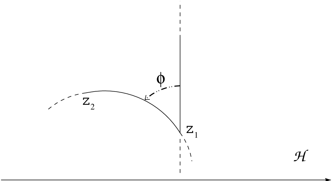
The differential of this function is now a well-defined $1$ -form on $C_{2,0}$ which we can pull-back to the configuration space corresponding to the whole graph with the help of the natural projection $\pi_{e}$ associated to each edge $e=(z_{i},z_{j})$ of $\Gamma$

\begin{array}[]{rccc}\pi_{e}\colon&C_{n,\bar{n}}&\longrightarrow&C_{2,0}\\ &(z_{1},\ldots,z_{\bar{n}})&\mapsto&(z_{i},z_{j})\end{array}

to obtain $d\phi_{e}:=\pi_{e}^{*}\,d\phi\in\Omega^{1}(C_{n,\bar{n}})$ . The form that appears in the definition of the weight $w_{\Gamma}$ can now be defined as

\omega_{\Gamma}:=\bigwedge_{e\in\Gamma}d\phi_{e}

where the ordering of the $1$ -forms in the product is the one induced on the set of all edges by the ordering on the (first) vertices and the ordering on the set $\Star(v)$ of edges emerging from the vertex $v$ . We want to remark hereby that, as long as we consider graphs with $2n+\bar{n}-2$ edges, the degree of the form matches exactly the dimension of the space over which it has to be integrated, which gives us a real valued weight.

This geometric construction has a more natural interpretation if one derives the Kontsevich formula for the star product from a path integral approach, as it was done for the first time in [CF1].

For the weights to be well-defined, we also have to require that the integrals involved converge. However, as the geometric construction of $\phi$ suggests, as soon as two points approach each other, the differential form $d\phi$ is not defined. The solution to this problem has already been given implicitly in (5.1): the differential form is not integrated over the open configuration space, but on a suitable compact space whose definition and properties are contained in the following

Lemma 5.3.

For any configuration space $C_{n,\bar{n}}$ (resp. $C_{n}$ ) there exists a compact space $\bar{C}_{n,\bar{n}}$ (resp. $\bar{C}_{n}$ ) whose interior is the open configuration space and such that the projections $\pi_{e}$ , the angle map $\phi$ and thus the differential form $\omega_{\Gamma}$ extend smoothly to the corresponding compactifications.

The compactified configuration spaces are (compact) smooth manifolds with corners. We recall that a smooth manifold with corner of dimension $m$ is a topological Hausdorff space $M$ which is locally homeomorphic to ${\mathbb{R}}^{m-n}\times{\mathbb{R}}_{+}^{n}$ with $n=0,\ldots,m$ . The points $x\in M$ whose local expression in some (and thus any) chart has the form $x_{1},\ldots,x_{m-n},0,\ldots,0)$ are said to be of type $n$ and form submanifolds of $M$ called strata of codimension $n$ .

The general idea behind such a compactification is that the naive approach of considering the closure of the open space in the cartesian product would not take into account the different speeds with which two or more points “collapse” together on the boundary of the configuration space.

For a more detailed description of the compactification we refer the reader to [FMP] for an algebraic approach and to [AS] and [BT] for an explicit description in local coordinates. More recently Sinha [S] gave a simplified construction in the spirit of Kontsevich’s original ideas. In [AMM] the orientation of such spaces and of their codimension one strata – whose relevance will be clarified in the following – is discussed.

Finally, the integral in (5.1) is well-defined and yields a weight $w_{\Gamma}\in{\mathbb{R}}$ for any admissible graph $\Gamma$ , since we defined $w_{\Gamma}$ to be non zero only when $\Gamma$ has exactly $2n+m-2$ edges, i.e. when the degree of $\omega_{\Gamma}$ matches the dimension of the corresponding configuration space.

5.2 The proof: Lemmas, Stokes’ theorem, Vanishing theorems

Having defined all the tools we will need, we can now give a sketch of the proof.

In order to verify that $U$ defines the required $L_{\infty}$ -morphism we have to check that the following conditions hold:

I

The first component of the restriction of $U$ to $\mathcal{V}$ is – up to a shift in the degrees of the two DGLAs – the natural map introduced in Section (3.3).
II

$U$ is a graded linear map of degree $0$ .
III

$U$ satisfies the equations for an $L_{\infty}$ -morphism defined in Section (4).

Lemma 5.4.

I The map

U_{1}\colon\mathcal{V}\longrightarrow\mathcal{D}

is the natural map that identifies each multivector field with the corresponding multiderivation.

Proof.

The set $\mathcal{G}_{1,\bar{n}}$ consist of only one element, namely the graph $\Gamma_{\bar{n}}$ with one vertex of the first type with $2\cdot 1+\bar{n}-2=\bar{n}$ arrows with an equal number of vertices of the second type as endpoints.

To each $k$ -vector field $\xi$ we associate thus the multidifferential operator given by

U_{\Gamma_{\bar{n}}}(\xi)(f_{\bar{1}},\ldots,f_{\bar{n}}):=w_{\Gamma_{\bar{n}}}\;\xi^{i_{\bar{1}},\ldots,i_{\bar{n}}}\;\partial_{i_{\bar{1}}}f_{\bar{1}}\cdots\partial_{i_{\bar{n}}}f_{\bar{n}}.

An easy computation shows that the integral of $\omega_{\Gamma_{\bar{n}}}$ over $\bar{C}_{1,\bar{n}}$ cancels the power of $\frac{1}{2\pi}$ and leaves us with the right weight

w_{\Gamma_{\bar{n}}}=\frac{1}{\bar{n}!}

we expect for $U_{1}$ to be the natural map that induces the HKR isomorphism. ∎

Lemma 5.5.

II The $n$ -th component

U_{n}:=\sum_{\bar{n}=1}^{\infty}\sum_{\Gamma\in\mathcal{G}_{n,\bar{n}}}w_{\Gamma}B_{\Gamma}

has the right degree for $U$ to be an $L_{\infty}$ -morphism.

Proof.

To each vertex $v_{i}$ with $\#\Star(v_{i})$ outgoing arrows corresponds an element of $\mathcal{V}^{r_{i}}=\widetilde{\mathcal{V}}^{r_{i}+1}$ where $r_{i}=\#\Star(v_{i})$ . On the other side, each graph with $\bar{n}$ vertices of the second type together with an $n$ -tuple of multivector fields gives rise to a differential operator of degree $s=\bar{n}-1$ . Since we consider only graphs with $2n+\bar{n}-2$ edges and this is equal by construction to

\sum_{i=1}^{n}\#\Star(v_{i}),

the degree of $U_{n}(\xi_{1},\ldots,\xi_{n})$ can be written as

s=(2n+\bar{n}-2)+1-n=\sum_{i=1}^{n}r_{i}+1-n

which is exactly the prescribed degree for the $n$ -th component of an $L_{\infty}$ -morphism.

Although the construction we gave in the previous section involves a tensor product of multivector fields, the signs and weights in $U_{n}$ are chosen in such a way that, upon symmetrization, it descends to the symmetric algebra. ∎

We come now to the main part of Kontsevich’s construction: the geometric proof of the formality.

First of all we have to extend our morphism $U$ to include also a $0$ -th component which represents the usual multiplication between smooth functions — the associative product we want to deform via the higher order corrections. We can now specialize the $L_{\infty}$ condition (4.2) to the case at hand, where $m_{0}$ $\widetilde{m}_{0}$ can be expressed in terms of of the Taylor coefficients $U_{n}$ as:

$\displaystyle\sum_{l=0}^{n}$	$\displaystyle\sum_{k=-1}^{m}\sum_{i=0}^{m-k}\varepsilon_{kim}\!\!\!\!\sum_{\sigma\in S_{l,n-l}}\!\!\!\!\!\varepsilon_{\xi}(\sigma)\;U_{l}\Big(\xi_{{\sigma\hbox{\tiny{$(1)$}}}},\ldots,\xi_{{\sigma\hbox{\tiny{$(l)$}}}}\Big)$	(5.2)
	$\displaystyle\Big(f_{0}{\vbox{\hbox{\tiny{$\otimes$}}}}\cdots{\vbox{\hbox{\tiny{$\otimes$}}}}f_{i-1}{\vbox{\hbox{\tiny{$\otimes$}}}}U_{n-l}(\xi_{{\sigma\hbox{\tiny{$(l+1)$}}}},\ldots,\xi_{{\sigma\hbox{\tiny{$(n)$}}}})(f_{i}{\vbox{\hbox{\tiny{$\otimes$}}}}\cdots{\vbox{\hbox{\tiny{$\otimes$}}}}f_{i+k}){\vbox{\hbox{\tiny{$\otimes$}}}}f_{i+k+1}{\vbox{\hbox{\tiny{$\otimes$}}}}\cdots{\vbox{\hbox{\tiny{$\otimes$}}}}f_{m}\Big)$
$\displaystyle=$	$\displaystyle\sum_{i\neq j=1}^{n}\varepsilon_{\xi}^{ij}\;U_{n-1}(\xi_{i}\circ\xi_{j},\xi_{1},\ldots,\widehat{\xi_{i}},\ldots,\widehat{\xi_{j}},\ldots,\xi_{n})(f_{0}{\vbox{\hbox{\tiny{$\otimes$}}}}\cdots{\vbox{\hbox{\tiny{$\otimes$}}}}f_{n}),$

where

-

$\{\xi_{j}\}_{j=1,\ldots,n}$ are multivector fields;
-

$f_{0},\ldots,f_{m}$ are the smooth functions on which the multidifferential operator is acting;
-

$S_{l,n-l}$ is the subset of $S_{n}$ consisting of $(l,n-l)$ -shuffles
-

the product $\xi_{i}\circ\xi_{j}$ is defined in such a way that the Schouten–Nijenhuis bracket can be expressed in terms of this composition by a formula similar to the one relating the Gerstenhaber bracket to the analogous composition $\circ$ on $\mathcal{D}$ given in 3.2.2;
-

the signs involved are defined as follows: $\varepsilon_{kim}:=(-1)^{k(m+i)}$ , $\varepsilon_{\xi}(\sigma)$ is the Koszul sign associated to the permutation $\sigma$ and $\varepsilon_{\xi}^{ij}$ is defined as in (4.2).

This equation encodes the formality condition since the l.h.s. corresponds to the Gerstenhaber bracket between multidifferential operators while the r.h.s. contains “one half” of the Schouten–Nijenhuis bracket; the differentials do not appear explicitly since on $\mathcal{V}$ we defined $\mathrm{d}$ to be identically zero, while on $\mathcal{D}$ it is expressed in terms of the bracket with the multiplication $\mathfrak{m}$ , which we included in the equation as $U_{0}$ .

For a detailed explanation of the signs involved we refer once more to [AMM].

We can now rewrite equation (5.2) in a form that involves again admissible graphs and weights to show that it actually holds. It should be clear from the previous construction of the coefficients $U_{k}$ that the difference between the l.h.s. and the r.h.s. of equation (5.2) can be written as a linear combination of the form

\sum_{\Gamma\in\mathcal{G}_{n,\bar{n}}}c_{\Gamma}U_{\Gamma}(\xi_{1},\ldots,\xi_{n})(f_{0}{\vbox{\hbox{\tiny{$\otimes$}}}}\cdots{\vbox{\hbox{\tiny{$\otimes$}}}}f_{n})

(5.3)

where the the sum runs in this case over the set of admissible graphs with $2n+\bar{n}-3$ edges. Equation (5.2) is thus fulfilled for every $n$ if these coefficients $c_{\Gamma}$ vanish for every such graph.

The main tool to prove the vanishing of these coefficients is the Stokes Theorem for manifolds with corners, which ensures that also in this case the integral of an exact form $\mathrm{d}\Omega$ on a manifold $M$ can be expressed as the integral of $\Omega$ on the boundary $\partial M$ . In the case at hand, this implies that if we choose as $\Omega$ the differential form $\omega_{\gamma}$ corresponding to an admissible graph, since each $d\phi_{e}$ is obviously closed and the manifolds $\bar{C}^{+}_{n,\bar{n}}$ are compact by construction, the following holds:

\int_{\partial\bar{C}^{+}_{n,\bar{n}}}\!\!\omega_{\Gamma}=\int_{\bar{C}^{+}_{n,\bar{n}}}\!\!d\,\omega_{\Gamma}=0.

(5.4)

We will now expand the l.h.s. of (5.4) to show that it gives exactly the coefficient $c_{\Gamma}$ occurring in (5.3) for the corresponding admissible graph.

First of all, we want to give an explicit description of the manifold $\partial\bar{C}^{+}_{n,\bar{n}}$ on which the integration is performed. Since the weights $w_{\Gamma}$ involved in (5.2) are set to vanish identically if the degree of the differential form does not match the dimension of the space on which we integrate, we can restrict our attention to codimension $1$ strata of $\partial\bar{C}^{+}_{n,\bar{n}}$ , which have the required dimension $2n+\bar{n}-3$ equal to the number of edges and thus of the $1$ -forms $d\phi_{e}$ .

In an intuitive description of the configuration space $\bar{C}_{n,\bar{n}}$ , the boundary represents the degenerate configurations in which some of the $n+\bar{n}$ points “collapse together”. The codimension $1$ strata of the boundary can thus be classified as follows:

•

strata of type S1, in which $i\geq 2$ points in the upper half plane $\mathcal{H}^{+}$ collapse together to a point still lying above the real line. Points in such a stratum can be locally described by the product

$C_{i}\times C_{n-i+1,\bar{n}}.$ (5.5)

where the first term stand for the relative position of the collapsing points as viewed “through a magnifying glass” and the second is the space of the remaining points plus a single point toward which the first $i$ collapse.
•

strata of type S2, in which $i>0$ points in $\mathcal{H}^{+}$ and $j>0$ points in ${\mathbb{R}}$ with $2i+j\geq 2$ collapse to a single point on the real line. The limit configuration is given in this case by

$C_{i,j}\times C_{n-i,\bar{n}-j+1}.$ (5.6)

These strata have a pictorial representation in Figure 7. In both cases the integral of $\omega_{\Gamma}$ over the stratum can be split into a product of two integrals of the form (5.1): the product of those $d\phi_{e}$ for which the edge $e$ connects two collapsing points is integrated over the first component in the decomposition of the stratum given by (5.5) resp. (5.6), while the remaining $1$ -forms are integrated over the second.

According to this description, we can split the integral in the l.h.s. of (5.4) into a sum over different terms coming from strata of type S1 and S2. Now we are going to list all the possible configurations leading to such strata to show that most of these terms vanish and that the only remaining terms are exactly those required to give rise to (5.2). We will not check directly that the signs we get by the integration match with those in (5.2), since we did not give explicitly the orientation of the configuration spaces and of their boundaries, but we refer once again the reader to the only paper completely devoted to the careful computation of all signs involved in Kontsevich’s construction [AMM].

Among the strata of type S1, we distinguish two subcases, according to the number $i$ of vertices collapsing. Since the integrals are set to vanish if the degree of the form does not match the dimension of the domain, a simple dimensional argument shows that the only contributions come from those graphs $\Gamma$ whose subgraph $\Gamma_{1}$ spanned by the collapsing vertices contains exactly $2i-3$ edges.

If $i=2$ there is only an edge $e$ involved and in the first integral coming from the decomposition (5.5) the differential of the angle function is integrated over $C_{2}\cong S^{1}$ and we get (up to a sign) a factor $2\pi$ which cancels the coefficient in (5.1). The remaining integral represents the weight of the corresponding quotient graph $\Gamma_{2}$ obtained from the original graph after the contraction of $e$ : to the vertex $j$ of type I resulting from this contraction is now associated the $j$ -composition of the two multivector fields that were associated to the endpoints of $e$ . Therefore, summing over all graphs and all strata of this subtype we get the r.h.s. of the desired equation (5.2).

If $i\geq 3$ , the integral corresponding to this stratum involves the product of $2i-3$ angle forms over $C_{i}$ and vanishes according to the following Lemma, which contains the most technical result among Kontsevich’s “vanishing theorems”.

The two possible situations are exemplified in Figure 8.

Lemma 5.6.

The integral over the configuration space $C_{n}$ of $n\geq 3$ points in the upper half plane of any $2n-3$ ( $=\dim C_{n}$ ) angle forms $d\phi_{e_{i}}$ with $i=1,\ldots n$ vanishes for $n\geq 3$

Proof.

The first step consists in restricting the integration to an even number of angle forms. This is achieved by identifying the configuration space $C_{n}$ with the subset of $\mathcal{H}^{n}$ where one of the endpoints of $e_{1}$ is set to be the origin and the second is bounded to lie on the unit circle (this particular configuration can always be achieved with the help of the action of the Lie group $G^{\prime}$ ). The integral decomposes then into a product of $d\phi_{e_{1}}$ integrated over $S^{1}$ and the remaining $2n-4=:2N$ forms integrated over the resulting complex manifold $U$ given by the isomorphism $C_{n}\cong S^{1}\times U$ . The claim is then a consequence of the following chain of equalities:

	$\displaystyle\int_{U}\bigwedge_{j=1}^{2N}d\arg(f_{j})=$	$\displaystyle\int_{U}\bigwedge_{j=1}^{2N}d\log\|f_{j}\|=\int_{\overline{U}}\mathcal{I}\Big(d\big(\log\|f_{1}\|\bigwedge_{j=2}^{2N}d\log\|z_{j}\|\big)\Big)=$		(5.7)
	$\displaystyle=$	$\displaystyle\int_{\overline{U}}d\mathcal{I}\Big(\big(\log\|f_{1}\|\bigwedge_{j=2}^{2N}d\log\|z_{j}\|\big)\Big)=0$		(5.7)

where we gave an expression for the angle function $\phi_{e_{j}}$ in terms of the argument of the (holomorphic) function $f_{j}$ (which is nothing but the difference of the coordinates of the endpoints of $e_{j}$ ).

The first equality is what Kontsevich calls a “trick using logarithms” and follows from the decompositions

d\arg(f_{j})=\frac{1}{2i}\,\big(d\log(f_{j})-d\log(\overline{f}_{j})\big)

and

d\log|f_{j}|=\frac{1}{2}\,\big(d\log(f_{j})+d\log(\overline{f}_{j})\big).

The product of $2N$ such expressions is thus a linear combination of products of $k$ holomorphic and $2N-k$ anti-holomorphic forms. A basic result in complex analysis ensures that, upon integration over the complex manifold $U$ , the only terms that do not vanish are those with $k=N$ . It is a straightforward computation to check that the non vanishing terms coming from the first decomposition match with those coming from the second.

In the second equality the integral of the differential form is replaced by the integration of a suitable $1$ -form with values in the space of distributions over the compactification $\overline{U}$ of $U$ . A final Lemma in [Ko2] shows that this map $\mathcal{I}$ from standard to distributional $1$ -forms commutes with the differential, thus proving the last step in (5.7). In [Kho], Khovanskii gave a more elegant proof of this result in the category of complete complex algebraic varieties, deriving the first equality rigorously on the set of non singular points of $X$ and resolving the singularities with the help of a local representation in polar coordinates. ∎

Finally, turning our attention to the strata of type S2, the same dimensional argument introduced for the previous case restricts the possible non vanishing terms to the condition that the subgraph $\Gamma_{1}$ spanned by the $i+j$ collapsing vertices (resp. of the first and of the second type) contains exactly $2i+j-2$ edges.

With the same definition as before for the quotient graph $\Gamma_{2}$ obtained by contracting $\Gamma_{1}$ , we claim that the only non vanishing contributions come from those graphs for which both graphs obtained from a given $\Gamma$ are admissible. In this case the weight $w_{\Gamma}$ will decompose into the product $w_{\Gamma_{1}}\cdot w_{\Gamma_{2}}$ which in general, by the conditions on the number of edges of $\Gamma$ and $\Gamma_{1}$ , does not vanish.

Since all other properties required by Definition 5.1 are inherited from $\Gamma$ , we have only to check that we do not get “bad edges” by contraction. The only such possibility is depicted in the graph on the right in Figure 9 and occurs when $\Gamma_{2}$ contains an edge which starts from a vertex of the second type: in this case the corresponding integral vanishes because it contains the differential of an angle function evaluated on the pair $(z_{1},z_{2})$ , where the first point is constrained to lie on the real line and such a function vanishes for every $z_{2}$ because the angle is measured w.r.t. the Poincaré metric (as it can be inferred intuitively from Figure 5).

The only non vanishing terms thus correspond to the case when we plug the differential operator corresponding to the subgraph $\Gamma_{1}$ as $k$ -th argument of the one corresponding to $\Gamma_{2}$ , where $k$ is the vertex of the second type emerging from the collapse. Summing over all such possibilities and having checked (up to a sign as usual) that we get the right weights, it should be clear that the contribution due to the strata of type S2 accounts for the l.h.s. of (5.2).

In conclusion, we have proved that the morphism $U$ is an $L_{\infty}$ -morphism and since its first coefficient $U_{1}$ coincides with the map $U_{1}^{(0)}$ given in Section 3.3 it is also a quasi-isomorphism and thus determines uniquely a star product given by (4.4) for any given bivector field $\pi$ on ${\mathbb{R}}^{d}$ .

6 From local to global deformation quantization

The content of this last section is based mainly on the work of Cattaneo, Felder and Tomassini [CFT1] (see also [CFT2] and [CF2]), who gave a direct construction of the quantization of a general Poisson manifold.

The Kontsevich formula, in fact, gives a quantization only for the case $M={\mathbb{R}}^{d}$ for any Poisson bivector field $\pi$ and can thus be adopted in the general case to give only a local expression of the star product.

The globalization Kontsevich sketched in [Ko2] was carried through in [Ko3] by abstract arguments, extending the formality theorem to the general case.

The works of Cattaneo, Felder and Tomassini instead give an explicit recipe to define the star product globally, in a similar way to what Fedosov has done in the symplectic category [Fed]. Also in their approach, the main tool is a flat connection ${\overline{D}}$ on a vector bundle over $M$ such that the algebra of the horizontal sections w.r.t. to ${\overline{D}}$ is a quantization of the Poisson algebra of the manifold.

We give now an outline of the construction, addressing the reader to [CFT1] for details and proofs.

In the first step, we introduce the vector bundle $E_{0}\to M$ of infinite jets of functions together with the canonical flat connection $D_{0}$ . The fiber $E_{0}^{x}$ over $x\in M$ is naturally a commutative algebra and inherits the Poisson structure induced fiberwise by the Poisson structure on ${C^{\infty}\!\!\left(M\right)}$ . The canonical map which associates to any globally defined function its infinite jet at each point $x$ is a Poisson isomorphism onto the Poisson algebra of horizontal sections of $E_{0}$ w.r.t. $D_{0}$ .

As the star product yields a deformation of the pointwise product on ${C^{\infty}\!\!\left(M\right)}$ , we need also a “quantum version” of the vector bundle and of the flat connection in order to find an analogous isomorphism. The vector bundle $E\to M$ is defined in terms of a section ${\phi}^{\mathit{aff}}$ of the fiber bundle ${M}^{\mathit{aff}}\to M$ , where ${M}^{\mathit{aff}}$ is the quotient of the manifold ${M}^{\mathit{coor}}$ of jets of coordinates systems on $M$ by the action of the group $\GL(d,{\mathbb{R}})$ of linear diffeomorphisms, namely $E:=({\phi}^{\mathit{aff}})^{*}\widetilde{E}$ where $\widetilde{E}$ is the bundle of ${\mathbb{R}}{\vbox{\hbox{\scriptsize{$[[\epsilon]]$}}}}$ -modules

{M}^{\mathit{coor}}\;\times_{\GL(d,{\mathbb{R}})}\;{\mathbb{R}}[[y^{1},\ldots,y^{d}]]{\vbox{\hbox{\scriptsize{$[[\epsilon]]$}}}}\to{M}^{\mathit{aff}}.

Since the section ${\phi}^{\mathit{aff}}$ can be realized explicitly by a collection of infinite jets at $0$ of maps $\phi_{x}\colon{\mathbb{R}}^{d}\to M$ such that $\phi_{x}(0)=x$ for every $x\in M$ (defined modulo the action of $GL(d,{\mathbb{R}})$ ), we can suppose for simplicity that we have fixed a representative $\phi_{x}$ of the equivalence class for each open set of a given covering, thus realizing a trivialization of the bundle $E$ . Therefore, from now on we will identify $E$ with the trivial bundle with fiber ${\mathbb{R}}[[y^{1},\ldots,Y^{d}]]{\vbox{\hbox{\scriptsize{$[[\epsilon]]$}}}}$ ; in this way $E$ realizes the desired quantization, since it is isomorphic (as a bundle of ${\mathbb{R}}{\vbox{\hbox{\scriptsize{$[[\epsilon]]$}}}}$ -modules) to the bundle $E_{0}{\vbox{\hbox{\scriptsize{$[[\epsilon]]$}}}}$ whose elements are formal power series with infinite jets of functions as coefficients.

In order to define the star product and the connection on $E$ , we have first to introduce some new objects whose existence and properties are byproducts of the formality theorem. Given a Poisson bivector field $\pi$ and two vector fields $\xi$ and $\eta$ on ${\mathbb{R}}^{d}$ , we define:

$\displaystyle P(\pi)$	$\displaystyle:=\sum_{k=0}^{\infty}\frac{\epsilon^{k}}{k!}\;U_{k}(\pi,\dots,\pi),$	(6.1)
$\displaystyle A(\xi,\pi)$	$\displaystyle:=\sum_{k=0}^{\infty}\frac{\epsilon^{k}}{k!}\;U_{k+1}(\xi,\pi,\dots,\pi),$
$\displaystyle F(\xi,\eta,\pi)$	$\displaystyle:=\sum_{k=0}^{\infty}\frac{\epsilon^{k}}{k!}\;U_{k+2}(\xi,\eta,\pi,\dots,\pi).$

A straightforward computation of the degree of the multidifferential operators on the r.h.s. of (6.1) shows that $P(\pi)$ is a (formal) bidifferential operator, $A(\xi,\pi)$ a differential operator and $F(\xi,\eta,\pi)$ a function. Indeed $P(\pi)$ is nothing but the star product associated to $\pi$ as introduced at the end of Section 4.

More precisely, $P$ , $A$ and $F$ are elements of degree resp. $0$ , $1$ and $2$ of the Lie algebra cohomology complex of (formal) vector fields with values in the space of local polynomial maps, i.e. multidifferential operators depending polynomially on $\pi$ : an element of degree $k$ of this complex is a map that sends $\xi_{1}\wedge\cdots\wedge\xi_{k}$ to a multidifferential operator $S(\xi_{1},\ldots,\xi_{k},\pi)$ (we refer the reader to [CFT1] for details). The differential $\delta$ on this complex is then defined by

	$\displaystyle\delta\,S(\xi_{1},\ldots,\xi_{k+1},\pi):=$	$\displaystyle\sum_{i=1}^{k+1}(-)^{i}\frac{d}{dt}\Big\|_{t=0}S(\xi_{1},\ldots,\hat{\xi}_{i},\ldots,\xi_{k+1},(\Phi_{\xi}^{t})_{*}\,\pi)\;+$		(6.2)
	$\displaystyle+$	$\displaystyle\sum_{i<j}(-)^{i+j}\;S({\left[{\,{\xi_{i}}\,,\,{\xi_{j}}\,}\right]},\xi_{1},\ldots,\hat{\xi}_{i},\ldots,\hat{\xi}_{j},x\ldots,\xi_{k+1},\pi)$		(6.2)

where a caret denotes as usual the omission of the corresponding argument and $\Phi_{\xi}^{t}$ is the flow of the vector field $\xi$ .

As the associativity condition on the star product, which can now be written in the form $P\circ(P\otimes\id-\id\otimes P)=0$ , follows from the formality theorem, the following equations are a corollary of the same result and can be proved with analogous computations:

•

$P(\pi)\circ(A(\xi,\pi)\otimes\id+\id\otimes A(\xi,\pi))=A(\xi,\pi)\circ P(\pi)+\delta P(\xi,\pi)$
•

$P(\pi)\circ(F(\xi,\eta,\pi)\otimes\id-\id\otimes F(\xi,\eta,\pi))=$

$=A(\xi,\pi)\circ A(\eta,\pi)-A(\eta,\pi)\circ A(\xi,\pi)+\delta A(\xi,\eta,\pi)$
•

$-A(\xi,\pi)\circ F(\eta,\zeta,\pi)-A(\eta,\pi)\circ F(\zeta,\xi,\pi)-A(\zeta,\pi)\circ F(\xi,\eta,\pi)=\delta F(\xi,\eta,\zeta,\pi)$

(6.3)

The first of these equations describes the fact that under the coordinate transformation induced by $\xi$ the star product $P(\pi)$ is changed to an equivalent one up to higher order terms. The last two equations will be used in the construction of the connection and its curvature, since they represent an analogous of the defining relations between a connection $1$ -form $A$ and its curvature $F_{A}$ .

Upon explicit computation of the configuration space integrals involved in the definition of the Taylor coefficients $U_{k}$ , we can also give the lowest order terms in the expansion of $P$ , $A$ and $F$ and their action on functions:

(i)

$P(\pi)(f\otimes g)=f\,g+\epsilon\,\pi(df,dg)+O(\epsilon^{2})$ ;
(ii)

$A(\xi,\pi)=\xi+O(\epsilon)$ , where we identify $\xi$ with a first order differential operator on the r.h.s.;
(iii)

$A(\xi,\pi)=\xi$ , if $\xi$ is a linear vector field;
(iv)

$F(\xi,\eta,\alpha)=O(\epsilon)$ ;
(v)

$P(\pi)(1\otimes f)=P(\pi)(f\otimes 1)=f$ ;
(vi)

$A(\xi,\pi)1=0$ .

Equations $i)$ and $v)$ where already introduced in Definition 2.1 as two of the defining conditions of a star product, while the ones involving $A$ are used to construct a connection $D$ on sections of $E$ .

A section $f\in\Gamma(E)$ is given locally by a map $x\to f_{x}$ where for every $y$ , $f_{x}(y)$ is a formal power series whose coefficients are infinite jets. On the space of such sections we can introduce a deformed product $\star$ which will give us the desired star product on ${C^{\infty}\!\!\left(M\right)}$ once we identify horizontal sections with ordinary functions. Denoting analogously by $\pi_{x}$ the push-forward by $\phi_{x}^{-1}$ of the Poisson bivector $\pi$ on ${\mathbb{R}}^{d}$ , we can define the deformed product through the formal bidifferential operator $P(\pi_{x})$ in the same way as $P(\pi)$ represents the usual star product:

(f\star g)_{x}(y):=f_{x}(y)\;g_{x}(y)+\epsilon\;\pi_{x}^{ij}(y)\frac{\partial f_{x}(y)}{\partial y^{i}}\frac{\partial g_{x}(y)}{\partial y^{j}}+O(\epsilon^{2}).

We can define the connection $D$ on $\Gamma(E)$ by

(D\,f)_{x}=d_{x}f+A_{x}^{M}f

where $d_{x}f$ is the de Rham differential of $f$ regarded as a function with values in ${\mathbb{R}}[[y^{1},\ldots,y^{d}]]{\vbox{\hbox{\scriptsize{$[[\epsilon]]$}}}}$ and the formal connection $1$ -form is specified by its action on a tangent vector $\xi$ by

A_{x}^{M}(\xi)=A(\hat{\xi}_{x},\pi_{x})

where $A$ is the operator defined in (6.1) evaluated on the multivector fields $\xi$ and $\pi$ expressed in the local coordinates system given by $\phi_{x}$ .

The important point is that since the coefficients $U_{k}$ of the formality map that appear in the definition of $P$ and $A$ are polynomial in the derivatives of the coordinate of the arguments $\xi$ and $\pi$ , all results holding for $P(\pi)$ and $A(\xi,\pi)$ are inherited by their formal counterparts. In particular equalities $i)$ and $v)$ above (together with the formality theorem from which they are derived) ensure that $\star$ is an associative deformation of the pointwise product on sections and equalities $ii)$ and $iii)$ can be used to prove that $D$ is indeed independent of the choice of $\phi$ and therefore induces a global connection on $E$ .

We can finally extend $D$ and $\star$ by the (graded) Leibniz rule to the whole complex of formal differential forms $\Omega^{\bullet}(E)=\Omega{M}\otimes_{{C^{\infty}\!\!\left(M\right)}}\Gamma(E)$ and use (6.3) to verify the following

Lemma 6.1.

Let $F^{M}$ be the $E$ -valued $2$ -form given by $x\to F_{x}^{M}$ where $F_{x}^{M}(\xi,\eta)=F(\hat{\xi}_{x},\hat{\eta}_{x},\pi_{x})$ for any pair of vector fields $\xi$ , $\eta$ . Then $F^{M}$ represent the curvature of $D$ and the two are related to each other and to the star product by the usual identities:

a)

$D(f\star g)=D(f)\star g+f\star D(g)$ ;
b)

$D^{2}(\cdot)={\left[{\,{F^{M}}\,\overset{\star}{,}\,{\cdot}\,}\right]}$ ;
c)

$D\,F^{M}=0$

Proof.

The identities follow directly from the relations (6.3), in which the star commutator ${\left[{\,{f}\,\overset{\star}{,}\,{g}\,}\right]}=f\star g-g\star f$ is already implicitly defined, once we identify the complex of formal multivector fields endowed with the differential $\delta$ with the complex of formal multidifferential operators with the de Rham differential. The map that realizes this isomorphism is explicitly defined in [CFT1]. ∎

A connection $D$ satisfying the above relations on a bundle $E$ of associative algebras is called a Fedosov connection with Weyl curvature $F$ : it is the kind of connection Fedosov introduced to give a global construction in the symplectic case. Following Fedosov, the last step to the required globalization is to deform $D$ into a new connection ${\overline{D}}$ which enjoys the same properties and moreover has zero Weyl curvature, so that we can define the complex $H^{k}(E,{\overline{D}})$ and in particular the (sub)algebra of horizontal sections $H^{0}(E,{\overline{D}})$ .

The construction of ${\overline{D}}$ relies on the following Lemmata.

Lemma 6.2.

Let $D$ be a Fedosov connection on $E$ with Weyl curvature $F$ and $\gamma$ an $E$ -valued $1$ -form, then

{\overline{D}}:=D+{\left[{\,{\gamma}\,\overset{\star}{,}\,{\cdot}\,}\right]}

is also a Fedosov connection whose Weyl curvature is $\overline{F}=F+D\,\gamma+\gamma\star\gamma$ .

Proof.

For any given section $f$ , a direct computation shows

	$\displaystyle{\overline{D}}^{2}f$	$\displaystyle={\left[{\,{F}\,\overset{\star}{,}\,{f}\,}\right]}+D{\left[{\,{\gamma}\,\overset{\star}{,}\,{f}\,}\right]}+{\left[{\,{\gamma}\,\overset{\star}{,}\,{Df}\,}\right]}+{\left[{\,{\gamma}\,\overset{\star}{,}\,{{\left[{\,{\gamma}\,\overset{\star}{,}\,{f}\,}\right]}}\,}\right]}=$
		$\displaystyle={\left[{\,{F}\,\overset{\star}{,}\,{f}\,}\right]}+{\left[{\,{D\gamma}\,\overset{\star}{,}\,{f}\,}\right]}+{\left[{\,{\gamma}\,\overset{\star}{,}\,{{\left[{\,{\gamma}\,\overset{\star}{,}\,{f}\,}\right]}}\,}\right]}={\left[{\,{F+D\,\gamma+\frac{1}{2}{\left[{\,{\gamma}\,\overset{\star}{,}\,{\gamma}\,}\right]}}\,\overset{\star}{,}\,{f}\,}\right]}$

where the last equality follows from the Jacobi identity for the star commutator, since every associative product induces a Lie bracket given by the commutator.

Applying ${\overline{D}}$ on the new curvature, we can check explicitly that

	$\displaystyle{\overline{D}}\Big(F+D\,\gamma+\frac{1}{2}{\left[{\,{\gamma}\,\overset{\star}{,}\,{\gamma}\,}\right]}\Big)$	$\displaystyle=D^{2}\gamma+\frac{1}{2}{\left[{\,{D\gamma}\,\overset{\star}{,}\,{\gamma}\,}\right]}-\frac{1}{2}{\left[{\,{\gamma}\,\overset{\star}{,}\,{D\gamma}\,}\right]}+{\left[{\,{\gamma}\,\overset{\star}{,}\,{F+D\gamma}\,}\right]}=$
		$\displaystyle={\left[{\,{F}\,\overset{\star}{,}\,{\gamma}\,}\right]}+{\left[{\,{\gamma}\,\overset{\star}{,}\,{F}\,}\right]}=0$

where we made use again of the (graded) Jacobi identity and of the (graded) skew-symmetry of ${\left[{\,{}\,\overset{\star}{,}\,{}\,}\right]}$ . ∎

Lemma 6.3.

Let $D$ be a Fedosov connection on a bundle $E=E_{0}{\vbox{\hbox{\scriptsize{$[[\epsilon]]$}}}}$ and $F$ its Weyl curvature and let

D=D_{0}+\epsilon D_{1}+\cdots\qquad\text{and}\qquad F=F_{0}+\epsilon F_{1}+\cdots

be their expansions as formal power series. If $F_{0}=0$ and the second cohomology of $E_{0}$ w.r.t. $D_{0}$ is trivial, there exist a $1$ -form $\gamma$ such that ${\overline{D}}$ has zero Weyl curvature.

Proof.

By the previous Lemma, the claim is equivalent to the existence of a solution to the equation

\overline{F}=F+D\,\gamma+\frac{1}{2}{\left[{\,{\gamma}\,\overset{\star}{,}\,{\gamma}\,}\right]}=0.

A solution can be explicitly constructed by induction on the order in $\epsilon$ , starting from $\gamma_{0}=0$ and assuming that $\gamma^{(k)}$ is a solution $\mod\epsilon^{k+1}$ . We can thus add to $\overline{F}^{k}=F+D\,\gamma^{(k)}+\frac{1}{2}{\left[{\,{\gamma^{(k)}}\,\overset{\star}{,}\,{\gamma^{(k)}}\,}\right]}$ the next term $\epsilon^{k+1}D_{0}\,\gamma_{k+1}$ to get $\overline{F}^{(k+1)}$ modulo higher terms. From $D\overline{F}^{(k)}+{\left[{\,{\gamma^{(k)}}\,\overset{\star}{,}\,{\overline{F}^{(k)}}\,}\right]}=0$ and the induction hypothesis $\overline{F}^{(k)}=0$ $\mod\epsilon^{k+1}$ we get $D_{0}\,\overline{F}^{(k)}=0$ . Since now $H^{2}(E_{0},D_{0})=0$ , we can invert $D_{0}$ to define $\gamma_{k+1}$ in terms of the lower order terms $\overline{F}^{(k)}$ in such a way that $\overline{F}^{(k+1)}=0$ is satisfied $\mod\epsilon^{k+2}$ , thus completing the induction step. ∎

Since in our case $D$ is a deformation of the natural flat connection $D_{0}$ on sections of the bundle of infinite jets, the hypothesis of the previous Lemma are satisfied and we can actually find a flat connection ${\overline{D}}$ which is still a good deformation of $D_{0}$ .

A last technical Lemma gives us an isomorphism between the algebra of the horizontal sections $H^{0}(E,{\overline{D}})$ and its non-deformed counterpart $H^{0}(E_{0},D_{0})$ , which in turn is isomorphic to the Poisson algebra ${C^{\infty}\!\!\left(M\right)}$ : this concludes the globalization procedure.

Only recently, Dolgushev [Do] gave a new proof of Kontsevich’s formality theorem for a general manifold. The main difference in this approach is that it is based on the use of covariant tensors unlike Kontsevich’s original proof, which is based on $\infty$ -jets of multidifferential operators and multivector fields and is therefore intrinsically local. In particular, he gave a solution of the deformation quantization problem for an arbitrary Poisson orbifold.

References

[Arb] E. Arbarello, “Introduction to Kontsevich’s Result on Deformation–Quantization of Poisson Structures,” in: Seminari di geometria algebrica, Pisa (1999), 5–20.
[Art] M. Artin, “Deformation of singularities,” Tata Institute of Fundamental Research, Bombay (1976).
[AMM] D. Arnal, D. Manchon, M. Masmoudi, “Choix de signes pour la formalité de M. Kontsevich,” math.QA/0003003.
[AS] S. Axelrod and I. Singer, “Chern-Simons perturbation theory II,” J. Diff. Geom. 39 (1994), no. 1, 173–213.
[BFFLS] F. Bayen, M. Flato, C. Fronsdal, A. Lichnerowicz and D. Sternheimer, “Quantum mechanics as a deformation of classical mechanics,” Lett. Math. Phys. 1 (1977), 521–530.
[BCG] M. Bertelson, M. Cahen and S. Gutt, “Equivalence of star products,” Class. Quantum Grav. 14 (1997), A93–A107.
[Bon] P. Bonneau, “Fedosov star products and one-differentiable deformations”. Lett. Math. Phys. 45 (1998), 363–376.
[BT] R. Bott and C. Taubes, “On the self-linking of knots. Topology and physics,” J. Math. Phys 35 (1994), no. 10, 5247–5287.
[BW] H. Bursztyn and A. Weinstein, “Poisson geometry and Morita equivalence,” math.SG/0402347
[C] A. Canonaco, “ $L_{\infty}$ -Algebras and Quasi–Isomorphisms,” in: Seminari di geometria algebrica, Pisa (1999), 67–86.
[CF1] A. S. Cattaneo and G. Felder, “A Path Integral Approach to the Kontsevich Quantization Formula,” Commun. Math. Phys. 212 (2000), 591–611.
[CF2] A. S. Cattaneo and G. Felder, “On the globalization of Kontsevich’s star product and the perturbative Poisson sigma model,” Prog. Theor. Phys. Suppl. 144 (2001), 38–53.
[CFT1] A. S. Cattaneo, G. Felder and L. Tomassini, “From local to global deformation quantization of Poisson manifolds,” Duke Math. J. 115 (2002), 329–352.
[CFT2] A. S. Cattaneo, G. Felder and L. Tomassini, “Fedosov connections on jet bundles and deformation quantization,” in: Deformation Quantization (ed. G. Halbout), IRMA Lectures in Mathematics and Theoretical Physics (ed. V. Turaev), de Gruyter, Berlin, (2002), 191–202.
[De] P. Deligne, “Déformations de l’Algèbre des Fonctions d’une Variété Symplectique : Comparaison entre Fedosov et DeWilde, Lecomte,” Selecta Math. N.S. 1 (1995), 667–697.
[DL] M. De Wilde and P. B. A. Lecomte, “Existence of star-products and of formal deformations of the Poisson Lie algebra of arbitrary symplectic manifolds,” Lett. Math. Phys. 7 (1983), no. 6, 487–496.
[DS] G. Dito and D. Sternheimer, “Deformation quantization: genesis, developments and metamorphoses,” in Deformation quantization, Strasbourg (2001), 9–54, IRMA Lect. Math. Theor. Phys., 1, de Gruyter, Berlin (2002).
[Do] V. Dolgushev, “Covariant and Equivariant Formality Theorems,” math.QA/0307212.
[Fed] B. Fedosov, “Deformation quantization and index theory,” Mathematical Topics 9, Akademie Verlag, Berlin (1996).
[FLS1] M. Flato, A. Lichnerowicz and D. Sternheimer, “Déformations $1$ -différentiables des algèbres de Lie attachées à une variété symplectique ou de contact,”. Compositio Math. 31 (1975), no. 1, 47–82.
[FLS2] M. Flato, A. Lichnerowicz and D. Sternheimer, “Crochet de Moyal-Vey et quantification,” C. R. Acad. Sci. Paris Sér. A-B 283 (1976), no. 1, Aii, A19–A24.
[FMP] W. Fulton and R. MacPherson, “Compactification of configuration spaces,” Annals of Mathematics 139 (1994), 183–225.
[Ger] M. Gerstenhaber, “The cohomology structure of an associative ring,” Ann. Math.(2) 78 (1963), 267–288.
[Gra] M. Grassi, “DG (Co)Algebras, DG Lie Algebras and $L_{\infty}$ Algebras,” in: Seminari di geometria algebrica, Pisa (1999), 49–66.
[Gro] H. J. Groenewold,”On the principles of elementary quantum mechanics,” Physics 12 (1946), 405–460.
[Gth] S. Gutt, Déformations formelles de l’algèbre des fonctions différentiables sur une variété symplectique, Thesis, Université Libre de Bruxelles (1980).
[GR] S. Gutt and J. Rawnsley, “Equivalence of star-products on a symplectic manifold: an introduction to Deligne’s Čech cohomology class,” J. Geom. Phys. 29 (1999), 347–392.
[HKR] G. Hochschild, B. Kostant and A. Rosenberg, “Differential forms on regular affine algebras,” Trans. Amer. Math. Soc. 02 (1962), 383–408.
[Ik] N. Ikeda, “Two-dimensional gravity and nonlinear gauge theory,” Ann. Phys. 235, (1994) 435–464.
[Kho] A. G. Khovanskii, “On a Lemma of Kontsevich,” Funktsional. Anal. i Prilozhen. 31 (1997), no. 4, 89–91; translation in Funct. Anal. Appl. 31 (1997), no. 4, 296–298.
[Kir] A. A. Kirillov, “Unitary representations of nilpotent Lie groups”, Russian Math. Surveys 17 (4), (1962), 53–104; “Elements of the theory of representations”, Springer, Berlin, (1976).
[Kos] B. Kostant, “Quantization and unitary representations”, Lects. in Mod. Anal. and Appl. III, Lecture Notes in Mathematics 170, Springer, New York (1970), 87–208.
[Ko1] M. Kontsevich, “Formality conjecture,” pp. 139–156 in: D. Sternheimer, J. Rawnsley and S. Gutt (eds.) Deformation theory and symplectic geometry, Ascona (1996), Math. Phys. Stud. 20, Kluwer Acad. Publ., Dordrecht (1997).
[Ko2] M. Kontsevich, “Deformation quantization of Poisson manifolds I,” math.QA/9709040.
[Ko3] M. Kontsevich, “Deformation quantization of algebraic varieties,” EuroConférence Moshé Flato 2000, Part III, Dijon. Lett. Math. Phys. 56 (2001), no. 3, 271–294.
[Ma] M. Manetti, “Deformation Theory Via Differential Graded Lie Algebras,” in: Seminari di geometria algebrica, Pisa (1999), 21–48.
[Mo] J. E. Moyal, “Quantum mechanics as a statistical theory,” Proc. Cambridge Phyl. Soc. (1949), 99–124.
[NT] R. Nest and R. Tsygan, “Algebraic index theorem,” Comm. Math. Phys. 172 (1995), 223–262; “Algebraic index theorem for families,” Adv. Math. 113 (1995), 151–205; “Formal deformations of symplectic manifolds with boundary,” J. Reine Angew. Math. 481 (1996), 27–54.
[SS] P. Schaller and T. Strobl, “Poisson structure induced (topological) field theories,” Modern Phys. Lett. A 9 (1994), no. 33, 3129–3136.
[SSt] M. Schlessinger and J. Stasheff, “The Lie algebra structure on tangent cohomology and deformation theory,” J. Pure Appl. Algebra 38 (1985), 313–322.
[Se] I. E. Segal, “Quantization of non-linear systems”, J. Math. Phys. 1 (1960), 468–488.
[S] D. Sinha, “Manifold theoretic compactifications of configuration spaces,” math.GT/0306385.
[So] J. M. Souriau, “Structure des Systèmes Dynamiques,” Dunod, Paris (1969)
[St] J. Stasheff, “The intrinsic bracket on the deformation complex of an associative algebra,” J. Pure Appl. Algebra, 89 (1993), 231–235.
[Ve] J. Vey, “Déformation du crochet de Poisson sur une variété symplectique,” Comment. Math. Helv. 50 (1975), 421–454.
[We] H. Weyl, “The theory of groups and quantum mechanics,” Dover, New York (1931), translated from “Gruppentheorie und Quantenmechanik,” Hirzel Verlag, Leipzig (1928); “Quantenmechanik und Gruppentheorie,” Z. Physik 46 (1927), 1–46.
[Wi] E. P. Wigner, “Quantum corrections for thermodynamic equilibrium,” Phys Rev. 40 (1932), 749–759.
[Xu] P. Xu, “Fedosov $\star$ -Products and Quantum Momentum Maps,” Comm. Math. Phys. 197 (1998), 167–197.

	$\displaystyle((f\star g)\star h)\;(x)$	$\displaystyle=e^{\left({\mathrm{i}}\frac{\hslash}{2}\;\alpha^{ij}{\frac{\partial}{\partial{x^{i}}}}{\frac{\partial}{\partial{z^{j}}}}\right)}(f\star g)(x)h(z)\Big\|_{x=z}=$
		$\displaystyle=e^{\left({\mathrm{i}}\frac{\hslash}{2}\;\alpha^{ij}({\frac{\partial}{\partial{x^{i}}}}+{\frac{\partial}{\partial{y^{i}}}}){\frac{\partial}{\partial{z^{j}}}}\right)}e^{\left({\mathrm{i}}\frac{\hslash}{2}\;\alpha^{kl}{\frac{\partial}{\partial{x^{k}}}}{\frac{\partial}{\partial{y^{l}}}}\right)}f(x)g(y)h(z)\Big\|_{x=y=z}=$
		$\displaystyle=e^{\left({\mathrm{i}}\frac{\hslash}{2}\;\alpha^{ij}{\frac{\partial}{\partial{x^{i}}}}{\frac{\partial}{\partial{z^{j}}}}+\alpha^{kl}{\frac{\partial}{\partial{y^{k}}}}{\frac{\partial}{\partial{z^{l}}}}+\alpha^{mn}{\frac{\partial}{\partial{x^{m}}}}{\frac{\partial}{\partial{y^{n}}}}\right)}f(x)g(y)h(z)\Big\|_{x=y=z}=$
		$\displaystyle=e^{\left({\mathrm{i}}\frac{\hslash}{2}\;\alpha^{ij}{\frac{\partial}{\partial{x^{i}}}}({\frac{\partial}{\partial{y^{j}}}}+{\frac{\partial}{\partial{z^{j}}}})\right)}e^{\left({\mathrm{i}}\frac{\hslash}{2}\;\alpha^{kl}{\frac{\partial}{\partial{y^{k}}}}{\frac{\partial}{\partial{z^{l}}}}\right)}f(x)g(y)h(z)\Big\|_{x=y=z}=$
		$\displaystyle=(f\star(g\star h))\;(x).$

Formality and Star Products

Abstract

Acknowledgments

1 Introduction

Physical motivation

Historical review of deformation quantization

Plan of the work

2 The star product

Definition 2.1.

Example 2.2.

Definition 2.3.

Lemma 2.4.

Proof.

3 Rephrasing the main problem: the formality

3.1 DGLA’s, L∞- algebras and deformation functors

Definition 3.1.

Definition 3.2.

Definition 3.3.

Definition 3.4.

Definition 3.5.

Definition 3.6.

Lemma 3.7.

Example 3.8.

3.2 Multivector fields and multidifferential operators

3.2.1 The DGLA 𝒱\mathcal{V}

Proposition 3.9.

3.2.2 The DGLA 𝒟\mathcal{D}

Proposition 3.10.

Proof.

Proposition 3.11.

3.3 The first term: U1U_{1}

4 Digression: what happens in the dual

5 The Kontsevich formula

5.1 Admissible graphs, weights and BΓB_{\Gamma}’s

Definition 5.1.

Example 5.2.

Lemma 5.3.

5.2 The proof: Lemmas, Stokes’ theorem, Vanishing theorems

Lemma 5.4.

Proof.

Lemma 5.5.

Proof.

Lemma 5.6.

Proof.

6 From local to global deformation quantization

Lemma 6.1.

Proof.

Lemma 6.2.

Proof.

Lemma 6.3.

Proof.

References

3.1 DGLA’s, L_∞- algebras and deformation functors

3.2.1 The DGLA $\mathcal{V}$

3.2.2 The DGLA $\mathcal{D}$

3.3 The first term: $U_{1}$

5.1 Admissible graphs, weights and $B_{\Gamma}$ ’s