A triple lacunary generating function for Hermite polynomials
Mathematics Subject Classifications: 05A15, 05A19, 05A40, 33C45
Abstract
Some of the classical orthogonal polynomials such as Hermite, Laguerre, Charlier, etc. have been shown to be the generating polynomials for certain combinatorial objects. These combinatorial interpretations are used to prove new identities and generating functions involving these polynomials. In this paper we apply Foata’s approach to generating functions for the Hermite polynomials to obtain a triple lacunary generating function. We define renormalized Hermite polynomials by
and give a combinatorial proof of the following generating function:
where and is the Catalan generating function. We also give an umbral proof of this generating function.
1 Introduction
The Hermite polynomials may be defined by the exponential generating function
| (1) |
In this paper we will give a combinatorial proof of an identity for Hermite polynomials. For our combinatorial interpretation, it is more convenient to take a different normalization of the Hermite polynomials, which makes all the coefficients positive. Therefore, we work with the polynomials , where , which have the generating function
All of our formulas for are easily converted into formulas for .
Foata [5] gave a combinatorial proof of Doetsch’s identity [2] giving a generating function for :
| (2) |
We will prove the following generating function for :
| (3) |
in which , where is the Catalan number generating function. Note that the formula can be written in terms of hypergeometric series:
where , and
is the rising factorial.
We prove formula (3) by two methods—umbral and combinatorial. In section 2, we define an umbra and study some of its properties and then give the umbral proof. An umbral proof of a generating function for is given in [6].
In section 3 we prove (3) combinatorially by showing that both sides enumerate the same weighted objects. We first describe the combinatorial interpretation of the Hermite polynomials and then give the details of the weighted objects counted by both sides of the formula.
By using these methods, it would be possible to give umbral and combinatorial proofs of a more general generating function for .
2 The Umbral Proof
Rota and Taylor in [7] laid a rigorous foundation for the classical umbral calculus. They consider a vector space of polynomials in several variables or “umbrae” and define the linear functional on it. A sequence is represented by an umbra if for all . In practice, the word is usually dropped and we simply write with the understanding that the functional has been applied. When we write , we mean . We consider formal power series with coefficients in a ring of formal power series .
Definition 2.1
A formal power series is admissible if for every monomial in , the coefficient of in is nonzero for only finitely many values of .
So, for example, is an admissible formal power series, while is not. Some computations similar to those of this section can be found in section 4 of Gessel [6].
2.1 The umbra and its properties
We now define an umbra whose relation to the Hermite polynomials will be described in the next section. In this section, we study some properties of this umbra that we will need. We define the umbra by so that
| (4) |
The following two formulas hold for .
Lemma 2.2
(i) For any admissible formal power series ,
(ii)
Proof. (i) We first observe that it is sufficient to prove that the formula holds for : If the formula is true for , then comparing coefficients of on both sides we get that the formula holds for . But this implies by linearity that the formula is true for all admissible formal power series . To prove the formula for , we have
(ii) We have
Corollary 2.3
For any admissible formal power series ,
Proof. As in the lemma, it is sufficient to prove the formula for . Here If we apply Lemma 2.2 (i) directly, we cannot eliminate the linear term in . So we introduce a parameter and rewrite as . We will choose a value for later. Now applying Lemma 2.2 (i) we get
Now we choose the value of to eliminate the term in on the right; i.e., we solve and get . Substituting this value of in the above expression and simplifying, we obtain that . By Lemma 2.2 (ii), this is equal to . But applying the definition of directly gives
Applying the corollary to gives the formula
| (5) |
which we will need in the next section.
2.2 Proof of the formula
To prove formula (3), we first express the Hermite polynomial in terms of the umbra . We have
Comparing the coefficients of on both sides, we get . Using this, we get
We follow the same procedure as in the proof of Corollary 2.3. We introduce a parameter and rewrite the last expression as . Now applying Lemma 2.2 (i) we get
| (6) |
In order to apply formula (5), we need to eliminate the linear term in . So we choose a value of that makes the coefficient of equal to zero. By solving a quadratic and taking the solution with a power series expansion, we get We know that the Catalan generating function is given by . In terms of this generating function, where . Using this value of to simplify expression (6), we get that
We know that satisfies the equation . Substituting and using the fact that , we obtain ; i.e., . This gives us
Applying formula (5) with , we get that
Then writing the second exponential function as a series and using (4), we obtain the final result:
Now we turn to the combinatorial method of proof. We begin with a combinatorial interpretation of the Hermite polynomials that will be used in the combinatorial proofs.
3 The Combinatorial Proof
We assume that the reader is familiar with enumerative applications of exponential generating functions, as described, for example, in [8, Chapter 5] and [1]. The product formula and the exponential formula for exponential generating functions discussed in these references play an important role in the combinatorial proofs.
3.1 Combinatorial interpretation of Hermite polynomials
The exponential generating function counts sets with one or two elements, where a one-element set is weighted . Then by the exponential formula, the coefficient of in , which is , is the generating polynomial for partitions of an -element set into blocks of size one or two, where each block of size one is weighted . (If we used as Foata did, instead of , we would need to attach a weight of to each two-element block and a weight of to each one element block.) It is convenient to represent these partitions as graphs in which the vertices in a two-element block are joined by an edge. We call these graphs, in which every vertex has degree at most one, matchings.
Thus the Hermite polynomial can be viewed as the generating polynomial for the number of vertices of degree zero over the set of all matchings on vertices, where each vertex of degree zero is assigned the weight . With this combinatorial interpretation we will prove the following formula:
| (7) |
We will describe the graphs enumerated by the left side of formula (7). Then we will describe the same graphs in terms of their connected components and use the product formula for exponential generating functions to complete the proof.
3.2 Graphs counted by the left side.
In order to give a combinatorial interpretation to , we must interpret , which counts matchings of a -element set, as counting labeled objects with labels. To accomplish this, we take labels and attach to each one three vertices marked , , and . Figure 1 shows a labeled vertex connected to three marked vertices.

Then counts graphs constructed by taking components like that in Figure 1, with labels 1, 2, …, and adding to them a matching of the marked vertices, where each unmatched marked vertex is weighted . Figure 2 shows such a graph.

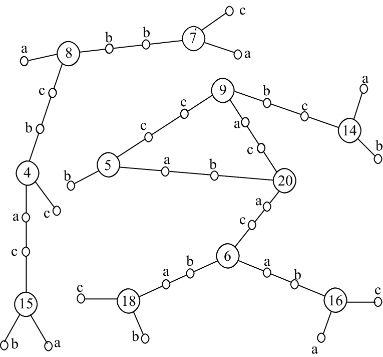
Let be the set of all graphs enumerated by the left side of formula (7). For a graph in , each vertex has degree one, two, or three. The trivalent vertices are labeled with the integers 1 to , where is the total number of trivalent vertices, and are weighted by the exponential generating function variable . The bivalent and monovalent vertices are marked with , , and ; the monovalent vertices have weight and the bivalent vertices have weight 1.
We first make a preliminary simplification of the graphs in : we eliminate all the bivalent marked vertices, moving their “marks” to the adjacent trivalent vertices.
More precisely, we think of each edge joining two trivalent vertices as consisting of two “half-edges”, each of which has a mark. Although we retain the monovalent vertices, we move their marks to the half-edge of the adjacent trivalent vertices. Note that some trivalent vertices now have loops. Figure 3, which shows the transformed version of the graph in Figure 2, should make this simplification clear.


We will express the generating function for graphs in as a product of three factors corresponding to connected components with no cycles, with exactly one cycle, and with at least two cycles. Note that a loop is a cycle.
3.3 Counting -trees
The graph in Figure 3 has three connected components. One component is a tree. The component with one cycle may be viewed as a cycle of trees. The third component may also be decomposed into trees and cycles. Thus the first step of our enumeration is to count the rooted trees from which we will construct our graphs, which we call -trees.
Definition 3.1
A -tree is a rooted tree with labeled trivalent internal vertices and unlabeled leaves in which the three half-edges incident with every internal vertex are marked with the letters , and , and one of the half-edges incident with the root has no matching half-edge.

Figure 4 shows a -tree. A special case of a -tree is the one with no internal vertices and no marks: it is simply a leaf with a half-edge attached to it.
We denote by the exponential generating function in for -trees where each internal vertex is weighted with and each leaf is weighted with . Let be the number of -trees with internal vertices. There are ways to draw such a tree (with the root at the top) by choosing an ordering of the two children of each internal vertex, so there are such drawings. But these drawings can be counted in another way. If we remove the labels and marks from such a drawing, we have a binary tree counted by the Catalan number . The marks can be added in ways and the labels in ways. Thus , so . Each such tree has leaves, so the exponential generating function for weighted -trees is . This relation to the Catalan generating function gives the equation as shown in section 2.2.
3.4 Acyclic components.
The connected components of graphs in with no cycles are trees. Such a tree appears in the lower left corner of Figure 3.
To count these trees we use a known method (see, e.g., [3]) for relating labeled unrooted trees of various types to rooted trees: we subtract the edge-rooted versions from the vertex-rooted versions.
First we count trees rooted at a trivalent vertex. In such a tree, the three half-edges at the root are joined to -trees. So we can construct such a rooted tree by taking an ordered triple of -trees, with exponential generating function , and a new root vertex with its three half-edges marked , , and , and attaching the first -tree to half-edge , the second to half-edge , and the third to half-edge . Thus the exponential generating function for these vertex-rooted trees is .
Next we count versions of these trees rooted at an edge joining two trivalent vertices. With the help of Figure 5 we see that the exponential generating function for such edge-rooted trees is .

An unrooted tree with trivalent vertices is counted times in the generating function for vertex-rooted trees and times in the generating function for edge-rooted trees. Thus the difference counts every unrooted tree once. A straightforward computation shows that can be expressed most simply as . Thus the exponential generating function for graphs whose connected components are trees is
| (8) |
As pointed out by the referee, other derivations of this generating function can be obtained by using the combinatorial interpretation of derivatives. Here is one such derivation: If is the generating function for these trees, then
| (9) |
since if we remove one of the monovalent vertices (weighted ) from a tree counted by , leaving an unmatched half-edge, we obtain a -tree with at least one trivalent vertex. Integrating with respect to , and using the fact that has constant term 0, we get
and this is easily checked to be equal to .
We also note that the coefficients of are given explicitly by
Now let us look at the connected components with one or more cycles. The two components other than the tree in Figure 3 are of this form. First we reduce these components by shrinking all the -trees present in them. Figure 6 illustrates this process.

As we see in the picture, the process of shrinking -trees leaves behind vertices weighted with which are now bivalent. We further reduce the components by eliminating these newly created bivalent vertices. Figure 7 shows what we get after this further reduction.

Thus we get either circles with no vertices or components (with multiple edges and loops) in which each vertex is trivalent. We will consider the two cases separately.
3.5 Components with one cycle.
If the reduction of a component of a graph in results in a circle, then the original component has exactly one cycle and each trivalent vertex on the cycle has a -tree attached at its third half-edge. The exponential generating function for directed cycles is . To count directed cycles with -trees attached, we replace by , and to add three marks to the half-edges of each vertex in the cycle, we multiply by . Finally, to undirect the cycles, we divide by 2. (Note that marking the half-edges for the cases and 2 destroys the symmetry that would prevent us from dividing by 2 before the marks are added.)
Thus the exponential generating function for cycles of -trees is
and so the exponential generating function for graphs whose connected components are cycles of -trees is
| (10) |
3.6 Components with more than one cycle.
The components of graphs in with more than one cycle reduce to connected graphs with only trivalent vertices. The connected graph on the left in Figure 7 is of this type. Rather than counting connected graphs of this type, as we did in the previous two sections, and then exponentiating, we count graphs, not necessarily connected, whose connected components are of this type. These graphs with labeled vertices are precisely the graphs counted by with no monovalent vertices. To see this, recall that in section 3.2 we described how each labeled vertex has three marked vertices attached to it and after constructing the matching on the marked vertices, the bivalent (or matched) marked vertices are eliminated as a preliminary simplification. If there are no unmatched marked vertices, the preliminary simplification gives a graph with only trivalent labeled vertices which have marks on their half-edges. Thus these graphs are counted by , the number of complete matchings of vertices. This number is 0 for odd and for .
We can recover the original graph from the reduced graph by introducing an ordered sequence of trivalent vertices on each edge, giving each new vertex marked half-edges and attaching a -tree to one of the half-edges. We can see this for the component with trivalent vertices in Figure 7 by tracing it back to its original component in Figure 3. Thus we get a factor for each of the edges in the reduced graph, where the 6 is the number of ways to specify the marks at a trivalent vertex. Hence the exponential generating function for graphs whose components have more than one cycle is
| (11) |
References
- [1] F. Bergeron, G. Labelle, and P. Leroux, Combinatorial Species and Tree-like Structures, Encyclopedia of Mathematics and its Applications, 67, Cambridge University Press, Cambridge, 1997, Translated from the 1994 French original by Margaret Readdy.
- [2] G. Doetsch, Integraleigenschaften der Hermiteschen Polynome, Math. Z. 32 (1930), 557–559.
- [3] P. Flajolet, D. Knuth, and B. Pittel, The first cycles in an evolving graph, Discrete Math. 75 (1989), 167–215.
- [4] D. Foata, A combinatorial proof of the Mehler formula, J. Combinatorial Theory Ser. A 24 (1978), 367–376.
- [5] D. Foata, Some Hermite polynomial identities and their combinatorics, Adv. in Appl. Math. 2 (1981), 250–259.
- [6] I. M. Gessel, Applications of the classical umbral calculus, Algebra Universalis 49 (2003), 397–434.
- [7] G.-C. Rota and B. D. Taylor, An introduction to the umbral calculus, Analysis, geometry and groups: a Riemann legacy volume, Hadronic Press, Palm Harbor, FL, 1993, pp. 513–525.
- [8] R. P. Stanley, Enumerative Combinatorics. Vol. 2, Cambridge University Press, Cambridge, 1999.