Heegaard diagrams and holomorphic disksThanks: PSO was partially supported by NSF grant numbers DMS-0234311, DMS-0111298, and FRG-0244663Thanks: ZSz was partially supported by NSF grant numbers DMS-0107792 and FRG-0244663, and a Packard Fellowship.
1. Introduction
Gromov’s theory of pseudo-holomorphic disks [39] has wide-reaching consequences in symplectic geometry and low-dimensional topology. Our aim here is to describe certain invariants for low-dimensional manifolds built on this theory.
The invariants we describe here associate a graded Abelian group to each closed, oriented three-manifold , the Heegaard Floer homology of . These invariants also have a four-dimensional counterpart, which associates to each smooth cobordisms between two such three-manifolds, a map between the corresponding Floer homology groups. In another direction, there is a variant which gives rise to an invariant of knots in .
1.1. Some background on Floer homology
To place Heegaard Floer homology into a wider context, we begin with Casson’s invariant. Starting with a Heegaard decomposition of an integer homology three-sphere , Casson constructs a numerical invariant which roughly speaking gives an obstruction to disjoining the character varieties of the two handlebodies inside the character variety for the Heegaard surface , c.f. [1], [94].
During the time when Casson introduced his invariants to three-dimensional topology, smooth four-dimensional topology was being revolutionized by the work of Donaldson [10], who showed that the moduli spaces of solutions to certain non-linear, elliptic PDEs – gauge theory equations which were first written down by physicists – revealed a great deal about the underlying smooth four-manifold topology. Indeed, he constructed certain diffeomorphism invariants, called Donaldson polynomials, defined by counting (in a suitable sense) solutions to these PDEs, the anti-self-dual Yang-Mills equations [11], [12], [16], [31], [53].
It was proved by Taubes in [99] that Casson’s invariant admits a gauge-theoretic interpretation. This interpretation was carried further by Floer [26], who constructed a homology theory whose Euler characteristic is Casson’s invariant. The construction of this instanton Floer homology proceeds by defining a chain complex whose generators are equivalence classes of flat connections over (or, more precisely, a suitably perturbed notion of flat connections, as required for transversality), and whose differentials count solutions to the anti-self-dual Yang-Mills equations. In fact, Floer’s instanton homology quickly became a central tool in the calculation of Donaldson’s invariants, see for example [67], [24], [15]. More specifically, under suitable conditions, the Donaldson invariant of a four-manifold separated along a three-manifold could be viewed as a pairing, in the Floer homology of , of relative Donaldson invariants coming from the two sides.
Floer’s construction seemed closely related to an earlier construction Floer gave in the context of Hamiltonian dynamics, known as “Lagrangian Floer homology” [27]. That theory – which is also very closely related to Gromov’s invariants for symplectic manifolds, c.f. [39] – associates to a symplectic manifold , equipped with a pair of Lagrangian submanifolds and (that in generic position, and satisfy certain topological restrictions), a homology theory whose Euler characteristic is the algebraic intersection number of and , but which gives a refined symplectic obstruction to disjoining the Lagrangians through exact Hamiltonian isotopies. More specifically, the generators for this chain complex are intersection points for and , and its differentials count holomorphic Whitney disks which interpolate between these intersection points, see also [33].
The close parallel between Floer’s two constructions, which take us back to Casson’s original picture, were further explored by Atiyah [3]. Atiyah conjectured that Floer’s instanton theory coincides with a suitably version of Floer’s Lagrangian theory, where one considers the character variety of as the ambient symplectic manifold, equipped with the Lagrangian submanifolds which are the character varieties of the two handlebodies. The Atiyah-Floer conjecture remains open to this day. For related results, see [17], [93], [105].
In 1994, there was another drastic turn of events in gauge theory and its interaction with smooth four-manifold topology, namely, the introduction of a new set of equations coming from physics, the Seiberg-Witten monopole equations [106]. These are a novel system of non-linear, elliptic, first-order equations which one can associate to a smooth four-manifold equipped with a Riemannian metric. Just as the Yang-Mills equations lead to Donaldson polynomials, the Seiberg-Witten equations lead to another smooth four-manifold invariant, the Seiberg-Witten invariant, c.f. [106], [66], [13], [52], [102]. These two theories seem very closely related. In fact, Witten conjectured a precise relationship between the two four-manifold invariants, see [106], [23], see also [55]. Moreover, many of the formal aspects of Donaldson theory have their analogues in Seiberg-Witten theory. In particular, it was natural to expect a similar relationship between their three-dimensional counterparts [64], [68], [63].
But now, a question arises in studying the three-dimensional theory: what is the geometric picture playing the role of character varieties in this new context? In attempting to formulate an answer to this question, we came upon a construction which has, as its starting point a Heegaard diagram for a three-manifold [72]. That is, is an oriented surface of genus , and and are a pair of -tuples of embedded, homologically linearly independent, mutually disjoint, closed curves. Thus, the and specify a pair of handlebodies and which bound , so that . Note that any oriented, closed three-manifold can be described by a Heegaard diagram. We associate to its -fold symmetric product , the space of unordered -tuples of points in . This space is equipped with a pair of -dimensional tori
| and |
The most naive numerical invariant in this context – the oriented intersection number of and – depends only on . However, by using the holomorphic disk techniques of Lagrangian Floer homology, we obtain a non-trivial invariant for three-manifolds, , whose Euler characteristic is this intersection number. In fact, there are some additional elaborations of this construction which give other variants of Heegaard Floer homology (denoted , , and , discussed below).
This geometric construction gives rise to invariants whose definition is quite different in flavor than its gauge-theoretic predecessors. And yet, it is natural to conjecture that certain variants give the same information as Seiberg-Witten theory. This conjecture, in turn, can be viewed as an analogue of the Atiyah-Floer conjecture in the Seiberg-Witten context. With this said, it is also fruitful to study Heegaard Floer homology and its structure independently from its gauge-theoretical origins.
1.2. Structure of this paper
Our aim in this article is to give a leisurely introduction to Heegaard Floer homology. We begin by recalling some of the details of the construction in Section 2. In Section 3, we describe some of the properties. Broader summaries can be found in some of our other papers (c.f. [71], [79]). In Section 4 we describe in further detail the relationship between Heegaard Floer homology and knots, c.f. [78], [80] and also the work of Rasmussen [87], [88]. We conclude in Section 5 with some problems and questions raised by these investigations.
We have not attempted to give a full account of the state of Heegaard Floer homology. In particular, we have said very little about the four-manifold invariants. We do not discuss here the Dehn surgery characterization of the unknot which follows from properties of Floer homology (see Corollary of [81], and also [56] for the original proof using Seiberg-Witten monopole Floer homology; compare also [38], [8], [35]). Another topic to which we have paid only fleeting attention is the close relationship between Heegaard Floer homology and contact geometry [76]. As a result, we do not have the opportunity to describe the recent results of Lisca and Stipsicz in contact geometry which result from this interplay, see for example [59].
1.3. Further remarks
The conjectured relationship between Heegaard Floer homology and Seiberg-Witten theory can be put on a more precise footing with the help of some more recent developments in gauge theory. For example, Kronheimer and Mrowka [50] have given a complete construction of a Seiberg-Witten-Floer package, which associates to each closed, oriented three-manifold a triple of Floer homology groups , , and which are functorial under cobordisms between three-manifolds. They conjecture that the three functors in this sequence are isomorphic to (suitable completions of) , and respectively. A different approach is taken in papers by Manolescu and Kronheimer, c.f. [62], [49].
2. The construction
We recall the construction of Heegaard Floer homology. In Subsection 2.1, we explain the construction for rational homology three-spheres (i.e. those three-manifolds whose first Betti number vanishes). In Subsection 2.2, we give an example which illustrates some of the subtleties involved in the Floer complex. In Subsection 2.4, we outline how the construction can be generalized for arbitrary closed, oriented three-manifolds. In Subsection 2.5, we sketch the construction of the maps induced by cobordisms, and in Subsection 2.6 we give preliminaries on the construction of the invariants for knots in . The material in Sections 2.1-2.4 is derived from [72]. The material from Subsection 2.5 is an account of the material starting in Section if [72] and continued in [73]. The material from Subsection 2.6 can be found in [78], see also [88].
2.1. Heegaard Floer homology for rational homology three-spheres
A genus handlebody is the three-manifold-with-boundary obtained by attaching one-handles to a zero-handle. More informally, a genus handlebody is homeomorphic to a regular neighborhood of a bouquet of circles in . The boundary of is a two-manifold with genus . If is any oriented three-manifold, for some we can write as a union of two genus handlebodies and , glued together along their boundary. A natural way of thinking about Heegaard decompositions is to consider self-indexing Morse functions
with one index critical point, one index three critical point, and index one (hence also index two) critical points. The space , then, is the preimage of the interval (with boundary the preimage of ); while is the preimage of . We orient as the boundary of .
Heegaard decompositions give rise to a combinatorial description of three-manifolds. Specifically, let be a closed, oriented surface of genus . A set of attaching circles for is a -tuple of homologically linearly independent, pairwise disjoint, embedded curves . A Heegaard diagram is a triple consisting of , where and are both complete sets of attaching circles for . From the Morse-theoretic point of view, the points in can be thought of as the points on which flow out of the index one critical points (with respect to a suitable metric on ), and the points in are points in which flow into the index two critical points.
In the opposite direction, a set of attaching circles for specifies a handlebody which bounds , and hence a Heegaard diagram specifies an oriented three-manifold . It is a classical theorem of Singer [98] that every closed, oriented three-manifold admits a Heegaard diagram, and if two Heegaard diagrams describe the same three-manifold, then they can be connected by a sequence of moves of the following type:
- •
isotopies: replace by a curve which is isotopic through isotopies which are disjoint from the other (); or, the same moves amongst the
- •
handleslides: replace by , which is a curve with the property that bound a pair of pants which is disjoint from the remaining (); or, the same moves amongst the
- •
stabilizations/destabilizations: A stabilization replaces by its connected sum with a genus one surface , and replaces and by and respectively, where and are a pair of curves supported in , meeting transversally in a single point.
Our goal is to associate a group to each Heegaard diagram, which is unchanged by the above three operations, and hence an invariant of the underlying three-manifold.
To this end, we will use a variant of Floer homology in the -fold symmetric product of a genus Heegaard surface , relative to the pair of totally real subspaces
| and |
That is to say, we define a chain complex generated by intersection points between and , and whose boundary maps count pseudo-holomorphic disks in . Again, it is useful to bear in mind the Morse-theoretic interpretation: an intersection point between and can be viewed as a -tuple of gradient flow-lines which connect all the index two and index one critical points. We denote the corresponding one-chain in by and call it a simultaneous trajectory.
Before studying the space of pseudo-holomorphic Whitney disks, we turn out attention to the algebraic topology of Whitney disks. Specifically, we consider the unit disk in , and let denote the arc where , and denote the arc where . Let denote the set of homotopy classes of Whitney disks, i.e. maps
Fix intersection points . There is an obvious obstruction to the existence of a Whitney disk which lives in . It is obtained as follows. Given and , consider the corresponding simultaneous trajectories and . The difference gives a closed loop in , whose homology class is trivial if there exists a Whitney disk connecting and . (Indeed, the condition is sufficient when .)
What this shows is that the space of intersection points between and naturally fall into equivalence classes labeled by elements in an affine space over .
There is another very familiar such affine space over : the space of structures over . Following Turaev [104], one can think of this space concretely as the space of equivalence classes of vector fields. Specifically, we say that two vector fields and over are homologous if they agree outside a Euclidean ball in . The space of homology classes of vector fields (which in turn are identified with the more standard definitions of structures, see [104], [37], [54]) is also an affine space over .
In order to link these two concepts, we fix a basepoint . Thinking of the Heegaard decomposition as a Morse function as described earlier, the base point describes a flow from the index zero to the index three critical point (for generic metric on ). Now, each tuple specifies a -tuple of connecting flows between the index one and index two critical points. Modifying the gradient vector field in a tubular neighborhood of these flow-lines so that it does not vanish there, we obtain a nowhere vanishing vector field over , whose homology class gives us a structure, depending on and . This gives rise to an assignment
It follows from the previous discussion that and can be connected by a Whitney disk if and only if .
Having answered the existence problem for Whitney disks, we turn to questions of its uniqueness (up to homotopy). For this, we turn once again to our fixed base-point . Given a Whitney disk connecting with , we can consider the intersection number between and the submanifold . This descends to homotopy classes to give a map
which is additive in the sense that , where here denotes the natural juxtaposition operation. The multiplicity can be modified by splicing in a copy of the two-sphere which generates (when ). Moreover, when is a rational homology sphere and , uniquely determines the homotopy class of – more generally, we have an identification . For the present discussion, though, we focus attention to the rational homology sphere case.
The most naive application of Floer’s theory would then give a -graded theory. However, the calculation of suggests that if we count each intersection number infinitely many times, we obtain a relatively -graded theory. Specifically, for a fixed structure over , let the set consist of intersection points which induce , with respect to the fixed base-point . Now we can consider the Abelian group freely generated by the set of pairs . We can give this space a natural relative -grading, by
| (1) |
where here is any homotopy class of Whitney disks which connects and , and denotes the Maslov index of , that is, the expected dimension of the moduli space of pseudo-holomorphic representatives of , see also [90]. If denotes the generator of (when ), then while , and hence is independent of the choice of . (It is easy to see that extends also to the cases where .)
Our aim will be to count pseudo-holomorphic disks. For this to make sense, we need to have a sufficiently generic situation, so that the moduli spaces are cut out transversally and, in particular,
| (2) |
To achieve this, we need to introduce a suitable perturbation of the notion of pseudo-holomorphic disks, see for instance Section of [72], see also [30], [33]. Specifically, for such a perturbation, we can arrange Equation (2) to hold for all homotopy classes with .
Indeed, since there is a one-parameter family of holomorphic automorphisms of the disks which preserve and the boundary arcs and , the moduli space admits a free action by , provided that is non-trivial. In particular, if has , then is a zero-dimensional manifold.
We then define a boundary map on by the formula
| (3) |
Here, can be thought of as either a count modulo of the number of points in the moduli space, in the case where we consider Floer homology with coefficients in or, in a more general case, to be an appropriately signed count of the number of points in the moduli space. For a discussion on signs, see [72], see also [29], [33].
By analyzing Gromov limits of pseudo-holomorphic disks, one can prove that , i.e. that is a chain complex.
It is easy to see that if a given homotopy class contains a holomorphic representative, then its intersection number is non-negative. This observation ensures that the subset generated by with is a subcomplex. It is also interesting to consider the quotient complex (which we can think of as generated by pairs with ). Note that all three complexes can be thought of as -modules, where
i.e. multiplication by lowers grading by two. Similarly, we can define a complex which is generated by the kernel of the -action on . We can think of directly as generated by intersection points between and , endowed with the differential
| (4) |
We now define Floer homology theories , , , , which are the homologies of the chain complexes , , , and respectively. Note that all of these groups are modules (where the action is trivial on ).
The main result of [72], then, is the following topological invariance of these theories:
Theorem 2.1.
The relatively -graded theories , , , and are topological invariants of the underlying three-manifold and its structure .
The content of the above result is that the invariants are independent of the various choices going into the definition of the homology theories. It can be broken up into parts, where one shows that the homology groups are identified as the Heegaard diagram undergoes the following changes:
- (1)
the complex structure over is varied
- (2)
the attaching circles are moved by isotopies (in the complement of )
- (3)
the attaching circles are moved by handle-slides (in the complement of )
- (4)
the Heegaard diagram is stabilized.
The first step is a direct adaptation of the corresponding fact from Lagrangian Floer theory (independence of the particular compatible almost-complex structure). To see the second step, we observe that any isotopy of the and can be realized as a sequence of exact Hamiltonian isotopies and metric changes over . The third step follows from naturality properties of the Floer homology theories (using a holomorphic triangle construction which we return to in Subsection 2.5), and a direct calculation in a special case (where handle-slides are made over a -fold connected sum of ). The final step can be seen as an invariance of the theory under a natural degeneration of the -fold symmetric product of the connected sum of with , as the connected sum neck is stretched, compare also [58], [41].
Although the study of holomorphic disks in general is a daunting task, holomorphic disks in symmetric products in a Riemann surface admit a particularly nice interpretation in terms of the underlying Riemann surface: indeed, holomorphic disks in the -fold symmetric product correspond to -fold branched coverings of the disk by a Riemann surface-with-boundary, together with a holomorphic map from the Riemann-surface-with-boundary into . This gives a geometric grasp of the objects under study, and hence, in many special cases, a way to calculate the boundary maps. In particular, it makes the model calculations used in the proof of handle-slide invariance mentioned above possible. We use it also freely in the following example.
2.2. An example
We give a concrete example to illustrate some of the familiar subtleties arising in the Floer complex. For simplicity, we stick to the case of . Moreover, since we have made no attempt to explain sign conventions, we consider the group with coefficients in
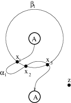
Of course, can be given a genus one Heegaard diagram, with two attaching circles and , which meet in a unique transverse intersection point. Correspondingly, the complex in this case has a single generator, and there are no differentials. Hence, . The diagram from Figure 1 is isotopic to this diagram, but now there are three intersections between and , , , and . By the Riemann mapping theorem, it is easy to see that . Thus, generates . Clearly, the chain complex changed under the isotopy since the combinatorics of the new Heegaard diagram is different (but, of course, its homology stayed the same).
But the chain complex can change for reasons more subtle than combinatorics. Consider the Heegaard diagram for illustrated in Figure 2.
For this diagram, there are two different chain complexes, depending on the choice of complex structure over (and the geometry of the attaching circles). We sketch the argument below.
First, it is easy to see that there are nine generators, corresponding to the points for . Again, by the Riemann mapping theorem applied to the region , there are holomorphic disks connecting to for for all . In a similar way, an inspection of Figure 2 reveals disks connecting to and to . However, the question of whether or not there is a holomorphic disk in (with ) connecting to is dictated by the conformal structures of the annuli in the diagram.
More precisely, consider the annular region illustrated in Figure 2. has a uniformization as a standard annulus with four points marked on its boundary, corresponding to the points , , , and . Let denote the angle of the arc in the boundary connecting and which is the image of the corresponding segment in under this uniformization; let denote the angle of the arc in the boundary connecting and which is the image of the corresponding segment in under the uniformization. Now, the question of whether there is a holomorphic disk in connecting to admits the following conformal reformulation. Consider the one-parameter family of conformal annuli with four marked boundary points obtained from by cutting a slit along starting at . The four boundary points are the images of , , and (counted twice) under a uniformization map. A four-times marked annulus which admits an involution (interchanging the two -arcs on the boundary) gives rise to a holomorphic disk connecting to . By analyzing the conformal angles of the arcs in this one-parameter family, one can prove that the mod count of the holomorphic is iff .
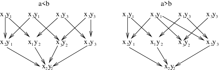
Proceeding in the like manner for the other homotopy classes, we see that in the regime where resp. , the chain complex has differentials listed on the left resp. right in Figure 3. These two complexes are different, but of course, they are chain homotopic.

2.3. Algebra
The reason for this zoo of groups , , , can be traced to a simple algebraic reason: (whose chain homotopy type is an invariant of ) is a finitely-generated chain complex of free -modules. All of the other groups are obtained from this from canonical algebraic operations. is the “localization” , is the cokernel of the localization map, and is the quotient .
Correspondingly, the various Floer homology groups are related by natural long exact sequences
| (5) |
and a more precise version of Theorem 2.1 states that both of the above diagrams are topological invariants of . The interrelationships between these groups is essential in the study of four-manifold invariants, as we shall see.
We can form another topological invariant, , which is the cokernel of appearing in Diagram (5).
2.4. Manifolds with
When , there are a number of additional technical issues which arise in the definition of Heegaard Floer homology. The crux of the matter is that there are homotopically non-trivial cylinders connecting and . Specifically, given any point , we have a subgroup of consisting of classes of Whitney disks with . This group, the group of “periodic classes,” is naturally identified with the cohomology group , and hence (provided ) . In particular, there are infinitely many homotopy classes of Whitney disks with a fixed multiplicity at a given point ; thus, the coefficients appearing in Equation (3) might a priori be infinite. One way to remedy this situation is to work with special Heegaard diagrams for . For example, in defining and , one can use Heegaard diagrams with the property that for which each non-trivial periodic class has a negative multiplicity at some . Such diagrams are called weakly admissible, c.f. Section of [72] for a detailed account, and also for a discussion of the stronger hypotheses needed for the construction of and .
Another related issue is that now, it is no longer true that the dimension of the space of holomorphic disks connecting depends only on the multiplicity at . Specifically, given a one-dimensional cohomology class , if and denotes the new element of obtained by letting the periodic class associated to act on , the Maslov classes of and are related by the formula:
where the right-hand-side is, of course, calculated over the three-manifold . Letting be the greatest common divisor of the integers of the form , the above discussion shows that the grading defined in Equation (1) gives rise to a relatively -graded theory.
With this said, there is an analogue of Theorem 2.1: when , the homology theories , , and (as calculated for special Heegaard diagrams) are relatively -graded topological invariants. Note that, there are only finitely many structures over for which is non-zero.
2.5. Maps induced by cobordisms
Cobordisms between three-manifolds give rise to maps between their Floer homology groups. The construction of these maps relies on the holomorphic triangle construction from symplectic geometry, c.f. [7], [33].
A bridge between the symplectic geometry construction and the four-manifold picture can be given as follows.
A Heegaard triple-diagram of genus is an oriented two-manifold and three -tuples , , and which are complete sets of attaching circles for handlebodies , , and respectively. Let , , and denote the three induced three-manifolds. A Heegaard triple-diagram naturally specifies a cobordism between these three-manifolds. The cobordism is constructed as follows.
Let denote the two-simplex, with vertices labeled clockwise, and let denote the edge from to , where . Then, we form the identification space
Over the vertices of , this space has corners, which can be naturally smoothed out to obtain a smooth, oriented, four-dimensional cobordism between the three-manifolds , , and as claimed.
We will call the cobordism described above a pair of pants connecting , , and . Note that if we give its natural orientation, then .
Fix , , . Consider the map
with the boundary conditions that , , and , and , , . Such a map is called a Whitney triangle connecting , , and . Two Whitney triangles are homotopic if the maps are homotopic through maps which are all Whitney triangles. We let denote the space of homotopy classes of Whitney triangles connecting , , and .
Using a base-point , we obtain an intersection number
If the space of homotopy classes of Whitney triangles is non-empty, then it can be identified with , in the case where .
As explained in Section of [72], the choice of base-point gives rise to a map
A structure over gives rise to a map
by the formula:
| (6) |
Under suitable admissibility hypotheses on the Heegaard diagrams, these sums are finite, c.f. Section of [72]. Indeed, there are induced maps on some of the other variants of Floer homology, and again, we refer the interested reader to that discussion for a more detailed account.
Let be a smooth, connected, oriented four-manifold with boundary given by where and are connected, oriented three-manifolds. We call such a four-manifold a cobordism from to . If is a cobordism from to , and is a structure, then there is a naturally induced map
where here denotes the restriction of to . This map is constructed as follows. First assume that is given as a collection of two-handles. Then we claim that in the complement of the regular neighborhood of a one-complex, can be realized as a pair-of-pants cobordism, one of whose boundary components is , the other which is , and the third of which is a connected sum of copies of . Next, pairing Floer homology classes coming from with a certain canonically associated Floer homology class on the connected sum of , we obtain a map using the holomorphic triangle construction as defined in Equation (6) to obtain a the desired map to . For the cases of one- and three-handles, the associated maps are defined in a more formal manner. The fact that these maps are independent (modulo an overall multiplication by ) of the many choices which go into their construction is established in [73].
Indeed, variants of this construction can be extended to the following situation (again, see [73]): if is a smooth, oriented cobordism from to , then there are induced maps (of modules) between the corresponding Heegaard Floer homology groups, which make the squares in the following diagrams commutate:
| (7) |
Naturality of the maps induced by cobordisms can be phrased as follows. Suppose that is a smooth cobordism from to and is a cobordism from to , then for fixed structures over which agree over , we have that
where here , , , (c.f. Theorem of [73]).
Sometimes, it is convenient to obtain topological invariants by summing over all structures. To this end, we write, for example,
It is convenient to have a corresponding notion for cobordisms, only in that case a little more care must be taken. For fixed and , we have that for all but finitely many , c.f. Theorem of [73], and hence there is a well-defined map
defined by
(note that the same construction works for , but it does not work for , : for a given , there might be infinitely many different for which is non-zero).
2.6. Doubly-pointed Heegaard diagrams and knot invariants
Additional basepoints give rise to additional filtrations on Floer homology. These additional filtrations can be given topological interpretations. We consider the case of two basepoints.
Specifically, a Heegaard diagram for equipped with two basepoints and gives rise to a knot in as follows. We connect and by a curve in and also by another curve in . By pushing and into and respectively, we obtain a knot . We call the data a doubly-pointed Heegaard diagram compatible with the knot . Given a knot in , one can always find such a Heegaard diagram.
This can be thought of from the following Morse-theoretic point of view. Let be an oriented three-manifold, equipped with a Riemannian metric and a self-indexing Morse function
with one index critical point, one index three critical point, and index one (hence also index two) critical points. The knot now is obtained from the union of the two flows connecting the index to the index critical points which pass through and . We call a Morse function as in the above construction one which is compatible with . Note also that an ordering of and is equivalent to an orientation on . However, the invariants we construct can be shown to be independent of the orientation of , see [78], [88].
The simplest construction now is to consider a differential on defined analogously to Equation (4), only now we count holomorphic disks for which . More generally, we use the reference point to construct the Heegaard Floer complex for , and then use the additional basepoint to induce a filtration on this complex. We describe this in detail for the case of knots in , and using the chain complex .
There is a unique function satisfying the relation
| (8) |
for any , and the additional symmetry
for all (compare, more generally, Equation (12)). (Alternatively, a more intrinsic characterization can be given in terms of relative structures on the knot complement.) Clearly, if appears in with non-zero multiplicity, then the homotopy class with admits a holomorphic representative, and hence . Thus, any filtration satisfying Equation (8) induces a filtration on the complex , by the rule that is the subcomplex generated by with .
It is shown in [78] and [88] that the chain homotopy type of this filtration is a knot invariant. More precisely, recall that a filtered chain complex is a chain complex , together with a sequence of subcomplexes indexed by , where . Our filtered complexes are always bounded, meaning that for all sufficiently large , and . A filtered map between chain complexes is one whose restriction to is contained in . Two filtered chain complexes are said to be have the same filtered chain type if there are maps and and and , all four of which are filtered maps, and are chain maps, and also we have that
| and |
The construction we mentioned earlier – counting holomorphic disks with can be thought of as the chain complex of the associated graded object
The homology of this is also a knot invariant. We return to properties of this invariant in Section 4.
3. Basic properties
We outline here some of the basic properties of Heegaard Floer homology, to give a flavor for its structure. We have not attempted to summarize all of its properties; for additional properties, see [71], [79], [73].
We focus on material which is useful for calculations: an exact sequence and rational gradings. We then turn briefly to properties of the maps induced on , which have some important consequences explained later, but they also shed light on the special role played by in Heegaard Floer homology. In Section 3.4 we give a few sample calculations. In Section 3.5, we describe one of the first applications of the rational gradings: a constraint on the intersection forms of four-manifolds which bound a given three-manifold, compare the gauge-theoretic analogue of Frøyshov [32]. Finally, in Subsection 3.6, we sketch how the maps induced by cobordisms give rise to an interesting invariant of closed, smooth four-manifolds with , which are conjectured to agree with the Seiberg-Witten invariants, c.f. [106].
3.1. Long exact sequences
An important calculational device is provided by the surgery long exact sequence. Long exact sequences of this type were first explored by Floer in the context of instanton Floer homology [28], [7], see also [97], [56].
Heegaard Floer homology satisfies a surgery long exact sequence, which we state presently. Suppose that is a three-manifold with torus boundary, and fix three simple, closed curves , , and in with
| (9) |
(where here the algebraic intersection number is calculated in , oriented as the boundary of ), so that resp. resp. are obtained from by attaching a solid torus along the boundary with meridian resp. resp. .
Theorem 3.1.
Let , , and be related as above. Then, there is a long exact sequence relating the Heegaard Floer homology groups:
The above theorem is proved in Theorem of [71]. A variant for Seiberg-Witten monopole Floer homology, with coefficients in is proved in [56].
The maps in the long exact sequence have a four-dimensional interpretation. To this end, note that there are two-handle cobordisms connecting to (where we view ). When we work with Heegaard Floer homology over the field , the map from to in the above exact sequence is the map induced by the corresponding cobordism , (i.e. obtained by summing the maps induced by all structures over ). When working over , though, one must make additional choices of signs to ensure that exactness holds.
3.2. Gradings
It is proved in Section of [71] that if is a rational homology three-sphere and is any structure over it, then , thus, this invariant is not a very subtle invariant of three-manifolds. However, extra information can still be gleaned from the interplay between and , with the help of some additional structure on Floer homology.
It is shown in [73] that when is an oriented rational homology three-sphere and is a structure over , the relative grading on the Heegaard Floer homology described earlier can be lifted to an absolute -grading. This gives is a -graded module over the polynomial algebra (where here is any of , , , or ),
where multiplication by lowers degree by two. In each grading, , is a finitely generated Abelian group.
The maps , , and in Diagram (5) preserve this -grading, and moreover, maps induced by cobordisms (again, denotes any of , , or ) respect the -grading in the following sense. If and are rational homology three-spheres, and is a cobordism from to , with structure , the map induced by the cobordism maps
for
| (10) |
where here denotes the Euler characteristic of , and denotes its signature. In fact (c.f. Theorem of [73]) the grading is uniquely characterized by the above property, together with the fact that .
The image of determines a function
(the “correction terms” of [79]) which associates to each structure the minimal -grading of any (non-zero) homogeneous element in in the image of .
Certain properties of the correction terms can be neatly summarized, with the help of the following definitions.
The three-dimensional homology bordism group is the set of equivalence classes of pairs where is a rational homology three-sphere, and is a structure over , and the equivalence relation identifies if there is a (connected, oriented, smooth) cobordism from to with for and , which can be endowed with a structure whose restrictions to and are and respectively. The connected sum operation endows this set with the structure of an Abelian group (whose unit is endowed with its unique structure).
There is a classical homomorphism
(see for instance [4]), defined as follows. Consider a rational homology three-sphere , and let be any four-manifold equipped with a structure with and . Then
where denotes the signature of the intersection form of .
It is shown in [79] that the numerical invariant descends to give a group homomorphism
which is a lift of . Moreover, is invariant under conjugation; i.e. .
The rational gradings can be introduced for three-manifolds with , as well, only there one must restrict to structures whose first Chern class is trivial. In this case, the gradings are fixed so that Equation (10) still holds. With these conventions, for example, for a three-manifold with , the Heegaard Floer homologies of for the structure with have a grading which takes its values in .
3.3. Maps on
As we have seen, for rational homology three-spheres, the structure of is rather simple. There are corresponding statements for the maps on induced by cobordisms.
3.4. Examples
We begin with some algebraic notions for describing Heegaard Floer homology groups. Let denote the graded -module , graded so that the element has grading .
A rational homology three-sphere is called an -space if has no torsion and the map from to is surjective. The Floer homology of an -space can be uniquely specified by its correction terms. That is, if is an -space, then
where here (and indeed throughout this subsection) the subscript denotes absolute grading, and
By a direct inspection of the corresponding genus one Heegaard diagrams, one can see that is an -space. Indeed, by a similar picture, all lens spaces are -spaces.
The absolute grading can also be calculated for lens spaces [79]. For example, for , there are two structures and with correction terms and respectively.
The Brieskorn homology sphere is also an -space, and it has .
However, is not an -space. Its Heegaard Floer homology is determined by
3.5. Intersection form bounds
The correction terms of a rational homology three-sphere constrain the intersection forms of smooth four-manifolds which bound , according to the following result, which is analogous to a gauge-theoretic result of Frøyshov [32]:
Theorem 3.2.
Let be a rational homology and be a smooth four-manifold which bounds with negative-definite intersection form. Then, for each structure over , we have that
| (11) |
The above theorem gives strong restrictions on the intersection forms of four-manifolds which bound a given three-manifold . In particular, if is an integral homology three-sphere, following a standard argument from Seiberg-Witten theory, compare [32], one can combine the above theorem with a number-theoretic result of Elkies [21] to show that if can be realized as the boundary of a smooth, negative-definite four-manifold, then ; moreover if , then if has negative-definite intersection form, then it must be diagonalizable.
3.6. Four-manifold invariants
The invariants associated to cobordisms can be used to construct an invariant for smooth, closed four-manifolds which is very similar in spirit to the Seiberg-Witten invariant for four-manifolds. Indeed, all known calculations support the conjecture that the two smooth four-manifold invariants agree.
Suppose that is a four-manifold with . We delete four-ball neighborhoods of two points in , and view the result as a cobordism from to , which we can further subdivide along a separating hypersurface into a union , with the following properties:
- •
is a cobordism from to with ,
- •
is a cobordism from to with ,
- •
restriction map is injective.
Such a separating hypersurface is called an admissible cut for .
Let denote the kernel of the map . Of course, this is isomorphic to the group , via an identification coming from the homomorphism from Equation (7). Since , the maps on induced by cobordisms are trivial (see Lemma of [73]), and in particular the image of the map
lies in the kernel of the map (c.f. Diagram (5). Moreover, the map
factors through the projection of to (the cokernel of the map from Diagram (5)). Thus, we can define
to be the composite:
where
is the natural isomorphism induced from .
The definition of depends on a choice of admissible cut for , but it is not difficult to verify [73] that is independent of this choice, giving a well-defined four-manifold invariant.
The element is non-trivial for only finitely many structures over . It vanishes for connected sums of four-manifolds with , c.f. Theorem of [73] (compare [12] and [106] for corresponding results for Donaldson polynomials and Seiberg-Witten invariants respectively). In fact, according to [77], if is a symplectic four-manifold for the canonical structure associated to the symplectic structure. This can be seen as an analogue of a theorem of Taubes [100] in the Seiberg-Witten context. Whereas Taubes’ theorem is proved by perturbing the Seiberg-Witten equations using a symplectic two-form, the non-vanishing theorem of is proved by first associating to a compatible Lefschetz pencil, which can be done according to a theorem of Donaldson, c.f. [14], blowing up to obtain a Lefschetz fibration, and then analyzing maps between Floer homology induced by two-handles coming from the singularities in the Lefschetz fibration, with the help of Theorem 3.1.
4. Knots in
We describe here constructions of Heegaard Floer homology applicable to knots. For simplicity, we restrict attention to knots in . This knot invariant was introduced in [78] and also independently by Rasmussen in [87], [88]. The calculations in Subsection 4.2 are based on the results of [80], [75], [83]. In Subsection 4.3, we discuss the fact that knot Floer homology detects the Seifert genus of a knot. This result is proved in [81]. The relationship with the four-ball genus is discussed in 4.4, where we discuss the concordance invariant of [82] and [88], and also the method of Owens and Strle [70]. Finally, in Subsection 4.5, we discuss an application to the problem of knots with unknotting number one from [74]. This application uses the Heegaard Floer homology of the branched double-cover associated to a knot.
4.1. Knot Floer homology
In Subsection 2.6, we described a construction which associates to an oriented knot in a three-manifold a filtration of the chain complex . Our aim here is to describe properties of this invariant when the ambient three-manifold is (although we will be forced to generalize to the case of knots in a connected sum of copies of , as we shall see later). In this case, a knot induces a filtration of the chain complex , whose homology is a single . With some loss of information, we can take the homology of the associated graded object, to obtain the “knot Floer homology”
Note that this can be viewed as one bigraded Abelian group
We call here the filtration level and (the grading induced from the Heegaard Floer complex ) the Maslov grading.
These homology groups satisfy a number of basic properties, which we outline presently. Sometimes, it is simplest to state these properties for , the homology with rational coefficients: .
The Euler characteristic is related to the Alexander polynomial of , by the following formula:
| (12) |
(it is interesting to compare this with [1], [64], and [25]). The sign conventions on the Euler characteristic here are given by
Unlike the Alexander polynomial, the knot Floer homology is sensitive to the chirality of the knot. Specifically, if denotes the mirror of (i.e. switch over- and under-crossings in a projection for ), then
| (13) |
Another symmetry these invariants enjoy is the following conjugation symmetry:
| (14) |
refining the symmetry of the Alexander polynomial.
These groups also satisfy a Künneth principle for connected sums. Specifically, let and be a pair of knots, and let denote their connected sum. Then,
| (15) |
(see Corollary of [78], and [88]). Of course, this can be seen as a refinement of the fact that the Alexander polynomial is multiplicative under connected sums of knots.
These invariants also satisfy a “skein exact sequence” (compare [28], [7], [79], [46]). To state it, we must generalize to the case of oriented links in . This can be done in the following manner: an -component oriented link in gives rise, in a natural way, to an -component oriented knot in . Specifically, we attach one-handles to , so that the two feet of each one-handle lie on different components of the link, and so that each link component meets at least one foot. Next, we form the connected sum of the various components of the link via standard strips which pass through the one-handles. In this way, we view the link invariant for an -component link as a knot invariant for the associated knot in .
In this manner, the homology of the associated graded object – the link Floer homology – is a sequence of graded Abelian groups , where here . If has an odd number of components, the Maslov grading is a -grading, while if it has an even number of components, the Maslov grading takes values in . As a justification for this convention, observe that the reflection formula, Equation (13), remains true in the context of links.
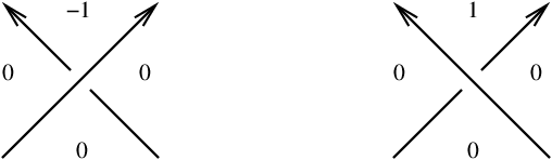
Suppose that is a link, and suppose that is a positive crossing of some projection of . Following the usual conventions from skein theory, there are two other associated links, and , where here agrees with , except that the crossing at is changed, while agrees with , except that here the crossing is resolved in a manner consistent with orientations, as illustrated in Figure 4. There are two cases of the skein exact sequence, according to whether or not the two strands of which project to belong to the same component of .

Suppose first that the two strands which project to belong to the same component of . In this case, the skein exact sequence reads:
| (16) |
where all the maps above respect the splitting of into summands (e.g. is mapped to ). Furthermore, the maps to and from drop degree by . The remaining map from to does not necessarily respect the absolute grading; however, it can be expressed as a sum of homogeneous maps, none of which increases absolute grading. When the two strands belong to different components, we obtain the following:
| (17) |
where denotes the four-dimensional vector space
where here are one-dimensional pieces supported in degree , while is a two-dimensional piece supported in degree . Moreover, the maps respect the decomposition into summands, where the summand of the middle piece is given by
The shifts in the absolute gradings work just as they did in the previous case.
4.2. Calculations of knot Floer homology
It is useful to have a concrete description of the generators of the knot Floer complex in terms of the combinatorics of a knot projection. In fact, the data we fix at first is an oriented knot projection (with at most double-point singularities), equipped with a choice of distinguished edge which appears in the closure of the unbounded region in the planar projection. We call this data a decorated projection for . We denote the planar graph of the projection by .
We can construct a doubly-pointed Heegaard diagram compatible with from a decorated projection of , as follows.
Let denote the other region which contains the edge in its closure, and let be the boundary of a regular neighborhood of , thought of as a one-complex in (i.e. if our projection has double-points, then has genus ); we orient as . We associate to each region , an attaching circle (which follows along the boundary of ). To each crossing in we associate an attaching circle as indicated in Figure 5. In addition, we let denote the meridian of the knot, chosen to be supported in a neighborhood of the distinguished edge .

Each vertex is contained in four (not necessarily distinct) regions. Indeed, it is clear from Figure 5, that in a neighborhood of each vertex , there are at most four intersection points of with circles corresponding to the four regions which contain . (There are fewer than four intersection points with if is a corner for the unbounded region .) Moreover, the circle corresponding to meets the circle in a single point (and is disjoint from the other circles). Placing one reference point and on each side of , we obtain a doubly-pointed Heegaard diagram for compatible with .
We can now describe the generators for the knot Floer homology in terms of the planar graph of the projection.
Definition 4.1.
A Kauffman state (c.f. [43]) for a decorated knot projection of is a map which associates to each vertex of one of the four in-coming quadrants, so that:
- •
the quadrants associated to distinct vertices are subsets of distinct regions in
- •
none of the quadrants is a corner of the distinguished regions or (whose closure contains the edge ).
If is a knot with a decorated projection, it is straightforward to see that the intersection points for the corresponding Heegaard diagram correspond to Kauffman states for the projection. Note that Kauffman states have an alternative interpretation, as maximal trees in the “black graph” associated to a checkerboard coloring of the complement of , c.f. [43].
We can also describe the filtration level and the Maslov grading of a Kauffman state in combinatorial terms of the decorated knot projection..
To describe the filtration level, note that the orientation on the knot associates to each vertex a distinguished quadrant whose boundary contains both edges which point towards the vertex . We call this the quadrant which is “pointed towards” at . There is also a diagonally opposite region which is “pointed away from” (i.e. its boundary contains the two edges pointing away from ). We define the local filtration contribution of at , denoted , by the following rule (illustrated in Figure 7), where denotes the sign of the crossing (which we recall in Figure 6):
The filtration level associated to a Kauffman state, then, is given by the sum
Note that the function is the -power appearing for the contribution of to the symmetrized Alexander polynomial, see [2], [44].


The Maslov grading is defined analogously. First, at each vertex , we define the local grading contribution . This local contributions is non-zero on only one of the four quadrants – the one which is pointed away from at . At this quadrant, the grading contribution is minus the sign of the crossing, as illustrated in Figure 8. Now, the grading of a Kauffman state is defined by the formula
A verification of these formulas can be found in Theorem of [80].
It is clear from the above formulas that if has an alternating projection, then is independent of the choice of state . It follows that if we use the chain complex associated to this Heegaard diagram, then there are no differentials in the knot Floer homology, and indeed, its rank is determined by its Euler characteristic. Indeed, by calculating the constant, we get the following result, proved in Theorem of [80]:
Theorem 4.2.
Let be an alternating knot in the three-sphere, and write its symmetrized Alexander polynomial as
and let denote its signature. Then, is supported entirely in dimension , and indeed
Thus, for alternating knots, this choice of Heegaard diagram is remarkably successful. However, in general, there are differentials one must grapple with, and these admit, at present, no combinatorial description in terms of Kauffman states. However, they do respect certain additional filtrations which can be described in terms of states, and this property, together with some additional tricks, can be used to give calculations of knot Floer homology groups in certain cases, c.f. [83], [18]. As a particular example, these filtrations are used in [83] to show that knot Floer homology of the eleven-crossing Kinoshita-Terasaka knot (a knot whose Alexander polynomial is trivial) differs from that of its Conway mutant.
In a different direction, some knots admit Heegaard diagrams on a genus one surface. For these knots, calculation of the differentials becomes a purely combinatorial matter, c.f. Section of [78] and also [87], [88], [36].
Sometimes, it is more convenient to use more abstract methods to calculate knot Floer homology. In particular, there is a relationship between knot Floer homology and the Heegaard Floer homology three-manifolds obtained by surgery along , c.f. [78], [88]. With the help of this relationship, we obtain the following structure for the knot Floer homology of a knot for which some positive surgery is an -space (proved in Theorem of [75]):
Theorem 4.3.
Suppose that is a knot for which there is a positive integer for which is an -space. Then, there is an increasing sequence of non-negative integers
with the property that , with the following significance. If we let
then unless for some , in which case and it is supported entirely in dimension .
For example, all (right-handed) torus knots satisfy the hypothesis of this theorem. (Recal that if denotes the right-handed torus knot, then is a lens space.) The knot Floer homology of the torus knot is illustrated in Figure 9. The above theorem can be fruitfully thought of from three perspectives: as a source of examples of knot Floer homology calculations (for example, a calculation of the knot Floer homology of torus knots), as a restriction on knots which admit -space surgeries (for example, it shows that if admits a lens space surgery, then all the coefficients of its Alexander polynomial satisfy ), or as a restriction on -spaces which can arise as surgeries on knots in , c.f. [75].

4.3. Knot Floer homology and the Seifert genus
A knot can be realized as the boundary of an embedded, orientable surface in . Such a surface is called a Seifert surface for , and the minimal genus of any Seifert surface for is called its Seifert genus, denoted . Of course, a knot has if and only if it is the unknot.
The knot Floer homology of detects the Seifert genus, and in particular it distinguishes the unknot, according to the following result proved in [81]. To state it, we first define the degree of the knot Floer homology to be the integer
Theorem 4.4.
For any knot , .
Given a Seifert surface of genus for , one can construct a Heegaard diagram for which all the points in have filtration level . This gives at once the bound
(this result is analogous to a classical bound on the genus of a knot in terms of the degree of its Alexander polynomial).
The inequality in the other direction is much more subtle, involving much of the theory described so far. First, one relates the degree of the knot Floer homology by a similar quantity defined using the Floer homology of the zero-surgery . Next, one appeals to a theorem of Gabai [35], according to which if is a knot with Seifert genus , then admits a taut foliation whose first Chern class is times a generator for . The taut foliation naturally induces a symplectic structure on , according to a result of Eliashberg and Thurston [20], which, according to a recent result of Eliashberg [19], [22] can be embedded in a closed symplectic four-manifold (indeed, one can arrange for to divide the four-manifold into two pieces with ). The non-vanishing of the four-manifold invariant for a symplectic four-manifold can then be used to prove that the Heegaard Floer homology of is non-trivial in the structure gotten by restricting the canonical structure of the ambient symplectic four-manifold – i.e. this is the structure belonging to the foliation . The details of this argument are given in [81].
Since the generators of knot Floer homology can be thought of from a Morse-theoretic point of view as simultaneous trajectories of gradient flow-lines, Theorem 4.4 immediately gives a curious Morse-theoretic characterization of the Seifert genus of , as the minimum over all Morse functions compatible with of the maximal filtration level of any simultaneous trajectory.
4.4. The four-ball genus
A knot can be viewed as a knot in the boundary of the four-ball, and as such, it can be realized as the boundary of a smoothly embedded oriented surface in the four-ball. The minimal genus of any such surface is called the four-ball genus of the knot, and it is denoted . Obviously, . In general, is quite difficult to calculate.
Lower bounds on can be obtained from Heegaard Floer homology. The construction involves going deeper into the knot filtration. Specifically, as explained explained in Subsection 2.6, the filtered chain homotopy type of the sequence of inclusions
is a knot invariant; passing to the homology of the associated graded object constitutes some loss of information. There is a quantity associated to the filtered complex which goes beyond knot Floer homology, and that is the integer which is defined by
The above inequality can be used to prove a property of which underscores its analogy with the correction terms described earlier. To put this result into context, we give a definition. Two knots and are said to be concordant if there is a smoothly embedded cylinder in with for . The set of concordance classes of knots can be made into an Abelian group, under the connected sum operation. It follows from Inequality (18), together with the additivity of under connected sums, that gives a homomorphism from the concordance group of knots to .
Another such homomorphism is provided by . In fact, according to Theorem 4.2,
| (19) |
when is alternating. By contrast, Theorem 4.3 gives many examples where Equation (19) fails. Indeed, combining Theorem 4.3 with Theorem 4.4 and Equation (12) and (18), we see that if is a knot which admits a positive surgery which is an -space surgery, then
and in particular, if , then
| (20) |
Note that the fact that is given by the above formula was conjectured by Milnor and first proved by Kronheimer and Mrowka using gauge theory [51].
In [60], see also [61] Livingston shows that properties of the concordance invariant (specifically, the fact that it is a homomorphism whose absolute value bounds the four-ball genus of , and satisfies Equation (20)) leads to the result that if is the closure of a positive on strands with crossings, then
The second of these equations was proved first by Rudolph [91] using the local Thom conjecture proved by Kronheimer and Mrowka [51]. Further links between the Thurston-Bennequin invariant and are explored by Plamenevskaya, see [86].
A different method for bounding is given by Owens and Strle in [70], where they describe a method using the correction terms for the branched double-cover of along , . Under favorable circumstances, their method gives an obstruction for Murasugi’s bound
| (21) |
to being sharp. Specifically, taking the branched double-cover of a surface in which bounds , one obtains a four-manifold which bounds . When is a surface with , the branched double is a four-manifold with definite intersection form, whose second Betti number is . Comparing this construction with the inequality from Theorem 3.2, one obtains restrictions on the correction terms of , which sometimes can rule out the existence of such surfaces .
4.5. Unknotting numbers
Recall that the unknotting number of a knot , denoted , is the the minimal number of crossing-changes required to unknot . An unknotting of can be realized as an immersed disk in which bounds . Resolving the self-intersections, one gets the inequality . However, there are circumstances where one needs better bounds (most strikingly, for any non-trivial slice knot). In [74], we describe an obstruction to knots having , in terms of the correction terms of the branched double-cover of .
This construction works best in the case where is alternating. In this case, the branched double-cover is an -space, c.f. [85]. A classical construction of Montesinos [65] shows that if , then can be obtained as surgery on another knot in , where here denotes the determinant of the knot (). On the one hand, correction terms for an -space which is realized as surgery (for some integer ) on a knot in satisfy certain symmetries (c.f. Theorem of [74]); on the other hand, the correction terms of the branched double-cover of an alternating knot can be calculated explicitly by classical data associated to an alternating projection of , c.f. [85]. Rather than recalling the result here, we content ourselves with illustrating an alternating knot (listed as in the Alexander-Briggs notation) whose unknotting number was previously unknown, but which can now be shown to have using these techniques.

5. Problems and Questions
The investigation of Heegaard Floer homology naturally leads us to the following problems and questions.
Perhaps the most important problem in this circle of ideas is the following:
Problem 1: Give a purely combinatorial calculation of Heegaard Floer homology or, more generally, the Heegaard Floer functor.
In certain special cases, combinatorial calculations can be given, for example [84], [80]. This problem would be very interesting to solve even for certain restricted classes of three-manifolds, for example for those which fiber over the circle, compare. [40], [95], [96] [9].
In a related direction, it is simpler to consider the case of knots in . Recall that in Section 4 we showed that the generators of the knot Floer complex can be thought of as Kauffman states.
Question 2: Is there a combinatorial description of the differential on Kauffman states whose homology gives the knot Floer homology of .
It is intriguing to compare this with Khovanov’s new invariants for links, see [46]. These invariants have a very similar structure to the knot Floer homology considered here, except that their Euler characteristic gives the Jones polynomial, see also [42], [47], [45], [48] [5]. Indeed, the similarities are further underscored by the work of E-S. Lee [57], who describes a spectral sequence which converges to a vector space of dimension , where is the number of components of , see also [89].
In a similar vein, it would be interesting to give combinatorial calculations of the numerical invariants arising from Heegaard Floer homology, specifically, the correction terms or the concordance invariant . An intriguing conjecture of Rasmussen [89] relates with a numerical invariant coming from Khovanov homology.
Problem 3: Establish the conjectured relationship between Heegaard Floer homology and Seiberg-Witten theory.
There are two approaches one might take to this problem. One direct, analytical approach would be to analyze moduli spaces of solutions to the Seiberg-Witten equations over a three-manifold equipped with a Heegaard decomposition. Another approach would involve an affirmative answer to the following question:
Question 4: Is there an axiomatic characterization of Heegaard Floer homology?
A Floer functor is a map which associates to any closed, oriented three-manifold a -graded Abelian group and to any cobordism from to a homorphism , which is natural under composition of cobordisms, and which induce exact sequences for triples of three-manifolds which are related as in the hypotheses of Theorem 3.1. It is interesting to observe that if is a natural transformation between Floer functors and to and , then if induces an isomorphism , then induces isomorphisms for all three-manifolds . This can be proved from Kirby calculus, following the outline laid out in [7]. We know from [56] that monopole Floer homology (taken with coefficients) is a Floer functor in this sense, and also (Theorem 3.1) that Heegaard Floer homology is a Floer functor. Unfortunately, this still falls short of giving an axiomatic characterization: one needs axioms which are sufficient to assemble a natural transformation .
Problem 5: Develop cut-and-paste techniques for calculating the Heegaard Floer homology of in terms of data associated to its pieces.
As a special case, one can ask how the knot Floer homology of a satellite knot can be calculated from data associated to the companion and the pattern. Of course, the Künneth principle for connected sums can be viewed as an example of this. Another example, of Whitehead doubling, has been studied by Eftekhary [18].
We have seen that the set of structures for which the Heegaard Floer homology of is non-trivial determines the Thurston norm of . It is natural to ask what additional topological information is contained in the groups themselves. It is possible that these groups contain further information about foliations over .
We specialize to the case of knot Floer homology. If is a fibered knot of genus , then it is shown in [76] that .
Question 6: If is a knot with genus and , does it follow that is fibered?
Calculations give some evidence that the answer to the above question is positive.
Question 7: If is a knot, is there an explicit relationship between the fundamental group of and the knot Floer homology ?
The above question is, of course, very closely related to the following:
Question 8: Is there an explicit relationship between the Heegaard Floer homology and the fundamental group of ?
For example, one could try to relate the Heegaard Floer homology with the instanton Floer homology of . (Note, though, that presently instanton Floer homology is defined only for a restricted class of three-manifolds, c.f. [7].) A link between Seiberg-Witten theory and instanton Floer homology is given by Pidstrygach and Tyurin’s monopole equations [23]. This connection has been successfully exploited in Kronheimer and Mrowka’s recent proof that all knots in have Property P [55].
The conjectured relationship with Seiberg-Witten invariants raises further questions. Specifically, Bauer and Furuta [34], [6] have constructed refinements of the Seiberg-Witten invariant which use properties of the Seiberg-Witten equations beyond merely their solution counts. Correspondingly, these invariants carry topological information about four-manifolds beyond their usual Seiberg-Witten invariants. A three-dimensional analogue is studied in work of Manolescu and Kronheimer, see [62], [49]
Question 9: Is there a refinement of the four-manifold invariant defined using Heegaard Floer homology which captures the information in the Bauer-Furuta construction?
In the opposite direction, it is natural to study the following:
Problem 10: Construct a gauge-theoretic analogue of knot Floer homology.
Recall from Section 3 that there is a class of three-manifolds whose Heegaard Floer homology is as simple as possible, the so-called -spaces. This class of three-manifolds includes all lens spaces, and more generally branched double-covers of alternating knots. The set of -spaces is closed under connected sums. According to [81], -spaces admit no (coorientable) taut foliations. A striking theorem of Némethi [69] characterizes those -spaces which are boundaries of negative-definite plumbings of spheres: they are the links of rational surface singularities. Note also that there is an analogous class of three-manifolds in the context of Seiberg-Witten monopole Floer homology, c.f. [56].
Question 11: Is there a topological characterization of -spaces (i.e. which makes no reference to Floer homology)?
References
- [1] S. Akbulut and J. D. McCarthy. Casson’s invariant for oriented homology -spheres, volume 36 of Mathematical Notes. Princeton University Press, Princeton, NJ, 1990. An exposition.
- [2] J. W. Alexander. Topological invariants of knots and links. Trans. Amer. Math. Soc., 30(2):275–306, 1928.
- [3] M. F. Atiyah. Floer homology, pages 105–108. Number 133 in Progr. Math. Birkhäuser, 1995.
- [4] M. F. Atiyah, V. K. Patodi, and I. M. Singer. Spectral asymmetry and Riemannian geometry. II. Math. Proc. Cambridge Philos. Soc, 78(3):405–432, 1975.
- [5] D. Bar-Natan. On Khovanov’s categorification of the Jones polynomial. Algebraic and Geometric Topology, 2:337–370, 2002.
- [6] S. Bauer and M. Furuta. A stable cohomotopy refinement of Seiberg-Witten invariants: I. math.DG/0204340.
- [7] P. Braam and S. K. Donaldson. Floer’s work on instanton homology, knots, and surgery. In H. Hofer, C. H. Taubes, A. Weinstein, and E. Zehnder, editors, The Floer Memorial Volume, number 133 in Progress in Mathematics, pages 195–256. Birkhäuser, 1995.
- [8] M. Culler, C. McA. Gordon, J. Luecke, and P. B. Shalen. Dehn surgery on knots. Ann. of Math, 125(2):237–300, 1987.
- [9] S. Donaldson and I. Smith. Lefschetz pencils and the canonical class for symplectic four-manifolds. Topology, 42(4):743–785, 2003.
- [10] S. K. Donaldson. An application of gauge theory to four-dimensional topology. J. Differential Geom., 18(2):279–315, 1983.
- [11] S. K. Donaldson. Irrationality and the -cobordism conjecture. J. Differential Geom., 26(1):141–168, 1987.
- [12] S. K. Donaldson. Polynomial invariants for smooth four-manifolds. Topology, 29(3):257–315, 1990.
- [13] S. K. Donaldson. The Seiberg-Witten equations and -manifold topology. Bull. Amer. Math. Soc. (N.S.), 33(1):45–70, 1996.
- [14] S. K. Donaldson. Lefschetz pencils on symplectic manifolds. J. Differential Geom., 53(2):205–236, 1999.
- [15] S. K. Donaldson. Floer homology groups in Yang-Mills theory, volume 147 of Cambridge Tracts in Mathematics. Cambridge University Press, Cambridge, 2002. With the assistance of M. Furuta and D. Kotschick.
- [16] S. K. Donaldson and P. B. Kronheimer. The Geometry of Four-Manifolds. Oxford Mathematical Monographs. Oxford University Press, 1990.
- [17] S. Dostoglou and D. A. Salamon. Self-dual instantons and holomorphic curves. Ann. of Math. (2), 139(3):581–640, 1994.
- [18] E. Eftekhary. Knot Floer homologies for pretzel knots. math.GT/0311419.
- [19] Y. M. Eliashberg. Few remarks about symplectic filling. math.SG/0311459.
- [20] Y. M. Eliashberg and W. P. Thurston. Confoliations. Number 13 in University Lecture Series. American Mathematical Society, 1998.
- [21] N. D. Elkies. A characterization of the lattice. Math. Res. Lett., 2(3):321–326, 1995.
- [22] J. B. Etnyre. On symplectic fillings. math.SG/0312091, 2003.
- [23] P. M. N. Feehan and T. G. Leness. monopoles, level-one Seiberg-Witten moduli spaces, and Witten’s conjecture in low degrees. Topology Appl., 124(2):221–326, 2002.
- [24] R. Fintushel and R. J. Stern. Seifert fibered homology three-spheres. Proc. of the London Math. Soc., 61:109–137, 1990.
- [25] R. Fintushel and R. J. Stern. Knots, links, and -manifolds. Invent. Math., 134(2):363–400, 1998.
- [26] A. Floer. An instanton-invariant for 3-manifolds. Comm. Math. Phys., 119:215–240, 1988.
- [27] A. Floer. Morse theory for Lagrangian intersections. J. Differential Geometry, 28:513–547, 1988.
- [28] A. Floer. Instanton homology and Dehn surgery. In H. Hofer, C. H. Taubes, A. Weinstein, and E. Zehnder, editors, The Floer Memorial Volume, number 133 in Progress in Mathematics, pages 77–97. Birkhäuser, 1995.
- [29] A. Floer and H. Hofer. Coherent orientations for periodic orbit problems in symplectic geometry. Math. Z., 212(1):13–38, 1993.
- [30] A. Floer, H. Hofer, and D. Salamon. Transversality in elliptic Morse theory for the symplectic action. Duke Math. J, 80(1):251–29, 1995.
- [31] R. Friedman and J. W. Morgan. Smooth four-manifolds and complex surfaces, volume 27 of Ergebnisse der Mathematik und ihrer Grenzgebiete (3). Springer-Verlag, Berlin, 1994.
- [32] K. A. Frøyshov. The Seiberg-Witten equations and four-manifolds with boundary. Math. Res. Lett, 3:373–390, 1996.
- [33] K. Fukaya, Y-G. Oh, K. Ono, and H. Ohta. Lagrangian intersection Floer theory—anomaly and obstruction. Kyoto University, 2000.
- [34] M. Furuta. Finite dimensional approximations in geometry. In Proceedings of the International Congress of Mathematicians, Vol. II (Beijing, 2002), pages 395–403, Beijing, 2002. Higher Ed. Press.
- [35] D. Gabai. Foliations and the topology of -manifolds III. J. Differential Geom., 26(3):479–536, 1987.
- [36] H. Goda, H. Matsuda, and T. Morifuji. Knot Floer homology of -knots. math.GT/0311084.
- [37] R. E. Gompf and A. I. Stipsicz. -manifolds and Kirby calculus, volume 20 of Graduate Studies in Mathematics. American Mathematical Society, 1999.
- [38] C. McA. Gordon and J. Luecke. Knots are determined by their complements. J. Amer. Math. Soc., 2(2):371–415, 1989.
- [39] M. Gromov. Pseudo holomorphic curves in symplectic manifolds. Inventiones Mathematicae, 82:307–347, 1985.
- [40] M. Hutchings and M. Sullivan. The periodic Floer homology of a Dehn twist. http://math.berkeley.edu/ hutching/pub/index.htm, 2002.
- [41] E. Ionel and T. H. Parker. Relative Gromov-Witten invariants. Ann. of Math. (2), 157(1):45–96, 2003.
- [42] M. Jacobsson. An invariant of link cobordisms from Khovanov’s homology theory. math.GT/0206303, 2002.
- [43] L. H. Kauffman. Formal knot theory. Number 30 in Mathematical Notes. Princeton University Press, 1983.
- [44] L. H. Kauffman. On knots. Number 115 in Annals of Mathematics Studies. Princeton University Press, 1987.
- [45] M. Khovanov. link homology I. math.QA/0304375.
- [46] M. Khovanov. A categorification of the Jones polynomial. Duke Math. J., 101(3):359–426, 2000.
- [47] M. Khovanov. An invariant of tangle cobordisms. math.QA/0207264, 2002.
- [48] M. Khovanov and L. Rozansky. Matrix factorizations and link homology. math.QA/0401268.
- [49] P. B. Kronheimer and C. Manolescu. Periodic Floer pro-spectra from the Seiberg-Witten equations. math.GT/0203243.
- [50] P. B. Kronheimer and T. S. Mrowka. Floer homology for Seiberg-Witten Monopoles. In preparation.
- [51] P. B. Kronheimer and T. S. Mrowka. Gauge theory for embedded surfaces. I. Topology, 32(4):773–826, 1993.
- [52] P. B. Kronheimer and T. S. Mrowka. The genus of embedded surfaces in the projective plane. Math. Research Letters, 1:797–808, 1994.
- [53] P. B. Kronheimer and T. S. Mrowka. Embedded surfaces and the structure of Donaldson’s polynomial invariants. J. Differential Geometry, pages 573–734, 1995.
- [54] P. B. Kronheimer and T. S. Mrowka. Monopoles and contact structures. Invent. Math., 130(2):209–255, 1997.
- [55] P. B. Kronheimer and T. S. Mrowka. Witten’s conjecture and Property P. math.GT/0311489, 2003.
- [56] P. B. Kronheimer, T. S. Mrowka, P. S. Ozsváth, and Z. Szabó. Monopoles and lens space surgeries. math.GT/0310164.
- [57] E. S. Lee. The support of the Khovanov’s invariants for alternating knots. math.GT/0201105, 2002.
- [58] A-M. Li and Y. Ruan. Symplectic surgery and Gromov-Witten invariants of Calabi-Yau 3-folds. Invent. Math., 145(1):151–218, 2001.
- [59] P. Lisca and A. I. Stipsicz. Heegaard Floer invariants and tight contact three-manifolds. math.SG/0303280, 2003.
- [60] C. Livingston. Computations of the Ozsváth-Szabó concordance invariant. math.GT/0311036.
- [61] C. Livingston. Splitting the concordance group of algebraically slice knots. Geom. Topol., 7:641–463, 2003.
- [62] C. Manolescu. Seiberg-Witten-Floer stable homotopy type of three-manifolds with . Geom. Topol., 7:889–932, 2003.
- [63] M. Marcolli and B-L. Wang. Equivariant Seiberg-Witten Floer homology. Comm. Anal. Geom., 9(3):451–639, 2001.
- [64] G. Meng and C. H. Taubes. SW=Milnor torsion. Math. Research Letters, 3:661–674, 1996.
- [65] J. M. Montesinos. Surgery on links and double branched covers of . In Knots, groups, and -manifolds (Papers dedicated to the memory of R. H. Fox), pages 227–259. Ann. of Math. Studies, No. 84. Princeton Univ. Press, Princeton, N.J., 1975.
- [66] J. W. Morgan. The Seiberg-Witten Equations and Applications to the Topology of Smooth Four-Manifold. Number 44 in Mathematical Notes. Princeton University Press, 1996.
- [67] J. W. Morgan, T. S. Mrowka, and D. Ruberman. The -Moduli Space and a Vanishing Theorem for Donaldson Polynomial Invariants. Number II in Monographs in Geometry and Topology. International Press, 1994.
- [68] T. S. Mrowka, P. S. Ozsváth, and B. Yu. Seiberg-Witten monopoles on Seifert fibered spaces. Comm. in Analysis and Geometry, 5(4):685–793, 1997.
- [69] A. Némethi. On the Ozsváth-Szabó invariant of negative definite plumbed -manifolds. math.GT/0310083.
- [70] B. Owens and S. Strle. Rational homology spheres and four-ball genus. math.GT/0308073, 2003.
- [71] P. S. Ozsváth and Z. Szabó. Holomorphic disks and three-manifold invariants: properties and applications. To appear in Annals of Math.. math.SG/0105202.
- [72] P. S. Ozsváth and Z. Szabó. Holomorphic disks and topological invariants for closed three-manifolds. To appear in Annals of Math.. math.SG/0101206.
- [73] P. S. Ozsváth and Z. Szabó. Holomorphic triangles and invariants for smooth four-manifolds. math.SG/0110169.
- [74] P. S. Ozsváth and Z. Szabó. Knots with unknotting number one and Heegaard Floer homology. math.GT/0401426.
- [75] P. S. Ozsváth and Z. Szabó. On knot Floer homology and lens space surgeries. math.GT/0303017.
- [76] P. S. Ozsváth and Z. Szabó. Heegaard Floer homologies and contact structures. math.SG/0210127, 2002.
- [77] P. S. Ozsváth and Z. Szabó. Holomorphic disk invariants for symplectic four-manifolds. math.SG/0201059, 2002.
- [78] P. S. Ozsváth and Z. Szabó. Holomorphic disks and knot invariants. math.GT/0209056, 2002.
- [79] P. S. Ozsváth and Z. Szabó. Absolutely graded Floer homologies and intersection forms for four-manifolds with boundary. Adv. Math., 173(2):179–261, 2003.
- [80] P. S. Ozsváth and Z. Szabó. Heegaard Floer homology and alternating knots. Geom. Topol., 7:225–254 (electronic), 2003.
- [81] P. S. Ozsváth and Z. Szabó. Holomorphic disks and genus bounds. math.GT/0311496, 2003.
- [82] P. S. Ozsváth and Z. Szabó. Knot Floer homology and the four-ball genus. Geom. Topol., 7:615–639, 2003.
- [83] P. S. Ozsváth and Z. Szabó. Knot Floer homology, genus bounds, and mutation. math.GT/0303225, 2003.
- [84] P. S. Ozsváth and Z. Szabó. On the Floer homology of plumbed three-manifolds. Geometry and Topology, 7:185–224, 2003.
- [85] P. S. Ozsváth and Z. Szabó. On the Heegaard Floer homology of branched double-covers. math.GT/0309170, 2003.
- [86] O. Plamenevskaya. Bounds for Thurston-Bennequin number from Floer homology. math.SG/0311090, 2003.
- [87] J. A. Rasmussen. Floer homology of surgeries on two-bridge knots. Algebr. Geom. Topol., 2:757–789 (electronic), 2002.
- [88] J. A. Rasmussen. Floer homology and knot complements. PhD thesis, Harvard University, 2003. math.GT/0306378.
- [89] J. A. Rasmussen. Khovanov homology and the slice genus. Preprint, 2003.
- [90] J. Robbin and D. Salamon. The Maslov index for paths. Topology, 32(4):827–844, 1993.
- [91] L. Rudolph. Quasipositivity as an obstruction to sliceness. Bull. Amer. Math. Soc. (N.S.), 29(1):51–59, 1993.
- [92] R. Rustamov. Calculation of Heegaard Floer homology for a class of Brieskorn spheres. math.SG/0312071, 2003.
- [93] D. Salamon. Lagrangian intersections, -manifolds with boundary, and the Atiyah-Floer conjecture. In Proceedings of the International Congress of Mathematicians, pages 526–536. Birkhäuser, 1994.
- [94] N. Saveliev. Lectures on the topology of -manifolds. de Gruyter Textbook. Walter de Gruyter & Co., Berlin, 1999. An introduction to the Casson invariant.
- [95] P. Seidel. The symplectic Floer homology of a Dehn twist. Math. Res. Lett., 3(6):829–834, 1996.
- [96] P. Seidel. Vanishing cycles and mutation. In European Congress of Mathematics, Vol. II (Barcelona, 2000), volume 202 of Progr. Math., pages 65–85. Birkhäuser, Basel, 2001.
- [97] P. Seidel. A long exact sequence for symplectic Floer cohomology. Topology, 42(5):1003–1063, 2003.
- [98] J. Singer. Three-dimensional manifolds and their Heegaard diagrams. Trans. Amer. Math. Soc., 35(1):88–111, 1933.
- [99] C. H. Taubes. Casson’s invariant and gauge theory. J. Differential Geom., 31(2):547–599, 1990.
- [100] C. H. Taubes. The Seiberg-Witten invariants and symplectic forms. Math. Research Letters, 1(6):809–822, 1994.
- [101] C. H. Taubes. More constraints on symplectic forms from Seiberg-Witten invariants. Math. Research Letters, 2(1):9–13, 1995.
- [102] C. H. Taubes. Seiberg Witten and Gromov invariants for symplectic -manifolds, volume 2 of First International Press Lecture Series. International Press, Somerville, MA, 2000. Edited by R. Wentworth.
- [103] C. H. Taubes. Seiberg-Witten invariants, self-dual harmonic 2-forms and the Hofer-Wysocki-Zehnder formalism. In Surveys in differential geometry, Surv. Differ. Geom., VII, pages 625–672. Int. Press, Somerville, MA, 2000.
- [104] V. Turaev. Torsion invariants of Spinc-structures on -manifolds. Math. Research Letters, 4:679–695, 1997.
- [105] K. Wehrheim. Anti-self-dual instantonts with Lagrangian boundary conditions. PhD thesis, Swiss Federal Institute of Technology, 2002.
- [106] E. Witten. Monopoles and four-manifolds. Math. Research Letters, 1:769–796, 1994.