A calculus for branched spines of 3-manifolds

By the calculus of Matveev-Piergallini, any two standard spines of $M$ are connected by a sequence of $2\rightarrow 3$-moves. Moreover, by a result of Y. Makovetsky (see [10]), it is possible to choose two sequences of positive $2\rightarrow 3$-moves connecting respectively $P_{1}$ and $P_{2}$ to the same standard spine $P$ of $M$. Since these sequences are composed by positive moves, they are branchable and hence they connect $P_{1}$ and $P_{2}$ to two different branched versions of the same spine $P$. Let us call these two branchings on $P$ respectively $b_{1}$ and $b_{2}$. In what follows, we will show that, using also branched versions of bubble-moves, lune and $2\to 3$-moves, it is possible to connect the branched spine $(P,b_{1})$ to $(P,b_{2})$.

Let $R^{+}_{1},..,R^{+}_{n}$ be the regions of $P$ oriented according to $b_{1}$; since $M$ is oriented, it makes sense to speak of the upper face and of the lower face of a region of $P$ with respect to a branching. Apply a bumping bubble-move as shown in the central part of Figure 7 to each region $R^{+}_{i}$ over which $b_{1}$ and $b_{2}$ differ, so that the bubbles are attached along the upper face of the region with respect to $b_{1}$ and call $R^{-}_{i}$ the new discs attached by the bubble-moves ($D$ in Figure 7). With an abuse of notation, exploiting the asymmetry of the bumping bubble-moves, we will call $R^{+}_{i}$ also the small disc ($D^{\prime}$ in Figure 7) created inside $R^{+}_{i}$ by the gluing of $R^{-}_{i}$. Note that the polyhedron $P^{\prime}_{1}$ obtained after the application of these moves contains $(P,b_{1})$ as a branched sub-polyhedron and in particular for each edge or vertex of $P$ there is a corresponding one in $P^{\prime}_{1}$; moreover, $P^{\prime}_{1}$ is necessarily non standard: we will sketch how to restore the standard setting in the end of the section. Analogously, let us call $P^{\prime}_{2}$ the polyhedron obtained by applying the above procedure using the branching $b_{2}$ to choose the upper faces of the regions. It is clear that $P^{\prime}_{1}$ and $P^{\prime}_{2}$ are branched version of the same polyhedron $P^{\prime}$; we keep calling $b_{1}$ and $b_{2}$ their branchings.

The idea of the proof is to slide the regions $R^{-}_{i}$ in $P^{\prime}_{1}$ to a final position where the roles of $R^{+}_{i}$ and of $R^{-}_{i}$ are exchanged and so, in particular, each $R^{+}_{i}$ appears as a bubble applied to the center of $R^{-}_{i}$, on its upper face: this connects $P^{\prime}_{1}$ and $P^{\prime}_{2}$ by a sequence of branched moves (not including bubble-moves).

Here and in what follows we will use the natural identification induced by a branched move between the regions of a polyhedron before and after the move as explained in the preceding section. Moreover, for the sake of simplicity, we suppose that the edges and the vertices we deal with are touched by distinct regions; this is not true in general but the proof can be easily adapted to the general case using local names for the regions around the edges and the vertices instead of the names $R^{\pm}_{*}$. We split the proof in two steps:

1. (1)

   For each edge $e$ of $P$ we use positive lune-moves near the corresponding edge $f$ in $P^{\prime}_{1}$ to create an edge such that if $e$ is touched by $R^{+}_{i}$, $R^{+}_{j}$ and $R^{+}_{k}$ in $P$ then the new edge is touched by $F(R^{+}_{i})$, $F(R^{+}_{j})$ and $F(R^{+}_{k})$, where $F(R^{+}_{*})=R^{+}_{*}$ if $b_{1}$ equals $b_{2}$ on $R^{+}_{*}$ in $P$ and is $R^{-}_{*}$ otherwise. This sequence of moves modifies $P^{\prime}_{1}$ creating some additional singular locus and hence producing a polyhedron no longer homeomorphic to $P^{\prime}$, but since it acts only near the center of the edges of $P^{\prime}_{1}$, the vertices of $P^{\prime}_{1}$ and hence of $P$ are identified with a subset of the vertices of the resulting polyhedron.

2. (2)

   For each vertex $v$ of $P$, we apply a sequence of branched moves to the corresponding vertex $w$ in the polyhedron obtained after Step $1$ to create a vertex such that if $R^{+}_{i}$, $R^{+}_{j}$, $R^{+}_{k}$, $R^{+}_{l}$, $R^{+}_{m}$ and $R^{+}_{n}$ are the regions of $P^{\prime}_{1}$ touching $v$ then the vertex is touched by the regions $F(R^{+}_{i})$, $F(R^{+}_{j})$, $F(R^{+}_{k})$, $F(R^{+}_{l})$, $F(R^{+}_{m})$ and $F(R^{+}_{n})$ (where, again, $F(R^{+}_{*})=R^{+}_{*}$ if $b_{1}$ and $b_{2}$ are equal in $P$ on $R^{+}_{*}$ and is $R^{-}_{*}$ otherwise). The sequence of moves we apply has also the effect of eliminating the extra singular locus created during the first step so that the final polyhedron we get is $P^{\prime}_{2}$.

Step 1. First of all, note that there are exactly $6$ possible different branchings on the neighborhood of an edge of a spine (of the $8$ possible $3$-uples of orientations on the regions touching the edge, two are to be excluded since of the branching condition). Moreover, each branching on an edge together with the orientation of $M$, produces a cyclic ordering of the regions touching it and a notion of up and down near it, so that we can define as shown in Figure 8 the regions of type $1$, $2$ and $3$ with respect to the branching on the edge.

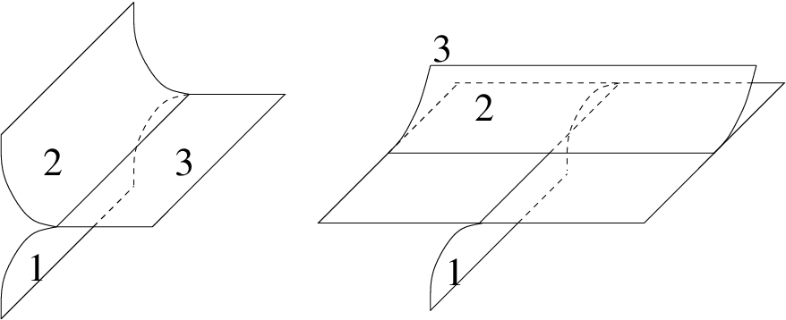
Let $e$ be an edge of $P$ where $b_{1}$ and $b_{2}$ are different, $f$ the corresponding edge in $P^{\prime}_{1}$ and let respectively $R^{+}_{i}$, $R^{+}_{j}$ and $R^{+}_{k}$ be the regions of type $1$, $2$ and $3$ with respect to the branching $b_{1}$ on $e$.

Suppose that $R^{+}_{i}$ is the only region touching $e$ on which $b_{1}$ and $b_{2}$ differ; we will now exhibit a sequence of $2$ positive bumping lune-moves near $f$ in $P^{\prime}_{1}$ which creates an edge touched by $R^{-}_{i}$, $R^{+}_{j}$ and $R^{+}_{k}$ and some additional singular locus which will be eliminated in Step $2$.

Since $R^{+}_{i}$ is oriented in the opposite way by $b_{1}$ and $b_{2}$, to get $P^{\prime}_{1}$ from $P_{1}$ we applied a bumping bubble-move over this region and created a disc $R^{-}_{i}$ on the upper (with respect to $b_{1}$) face of it. Apply a bumping lune-move to slide $R^{-}_{i}$ over a little disc contained in $R^{+}_{j}$ as shown in the upper part of Figure 9. This splits $f$ adding two new vertices and creates a new small disc and a new singular edge $f^{\prime}$ touched by $R^{-}_{i}$, $R^{+}_{j}$ and the disc itself. Apply now another bumping lune-move to slide $R^{+}_{i}$ over $R^{-}_{i}$ passing through the disc as shown in the lower-left part of Figure 9. The edge $f^{\prime}$ is split by two new vertices and a new small disc is created. With an abuse of notation we will call this new small disc $R^{-}_{i}$; indeed it can be viewed as a smooth continuation of $R^{-}_{i}$ over the edge separing them. After this move, the small straight edge connecting the two vertices in the lower-right part of Figure 9 is touched by the regions $R^{-}_{i}$, $R^{+}_{j}$ and $R^{+}_{k}$: we obtained the singular edge we were searching for. The side-effect of the sequence of moves just described is to create two pairs of new vertices positioned symmetrically with respect to the center of the edge: we will show in Step $2$ how to eliminate these vertices.

Suppose now that $b_{1}$ and $b_{2}$ differ only on $R_{j}$. We will now exhibit a sequence of $2$ sliding lune-moves near $f$ in $P^{\prime}_{1}$ creating a new edge $f^{\prime}$ touched by $R^{+}_{i}$, $R^{-}_{j}$ and $R^{+}_{k}$. Apply a sliding lune-move to push $R^{-}_{j}$ onto a little disc contained in $R^{+}_{k}$ and containing the center of $f$ in its boundary. The boundary of the little disc is formed by $f$ and another small singular edge $f^{\prime}$ (see the upper part of Figure 10). Then, we apply another sliding lune-move to push $R^{+}_{j}$ over $R^{-}_{j}$ near the center $f^{\prime}$ passing over the small disc. This creates another small disc “contained” in $R^{-}_{j}$ which, with an abuse of notation, we will call $R^{-}_{j}$. The sequence creates the edge touched by $R^{+}_{i}$, $R^{-}_{j}$ and $R^{+}_{k}$ we were searching for. Again, as a side-effect of the sequence, two pairs of new vertices disposed symmetrically with respect to the edge appear.

Let us now show how to conclude Step $1$ in the general case around $e$. Starting from $f$, we want to produce an edge in $P^{\prime}_{1}$ touched by the regions $F(R^{+}_{*})$ (where $F(R^{+}_{*})=R^{+}_{*}$ iff $b_{1}$ and $b_{2}$ do not differ on $R^{+}_{*}$). To do this, we “substitute” the regions one by one using the above sequences of moves. Consider the following algorithm:

1. (1)

   Let $X$ be the region of type $1$ with respect to the branching on $f$. If $X=F(R^{+}_{*})$ for some $R^{+}_{*}$ in $P^{\prime}_{1}$, go to $2$, otherwise apply the sequence of Figure 9 to $f$: this produces a new branched edge which we keep calling $f$ whose regions are still indicized by the three-uple $\{i,j,k\}$ and in which one more region is of the form $R^{-}_{*}=F(R^{+}_{*})$. Go to $2$.

2. (2)

   Let $Y$ be the region of type $2$ with respect to the branching on $f$. If $Y=F(R^{+}_{*})$ for some $R^{+}_{*}$ in $P^{\prime}_{1}$ stop, otherwise apply the sequence of Figure 10 to $f$: this produces a new branched edge which we keep calling $f$ whose regions are still indicized by the three-uple $\{i,j,k\}$ and in which one more region is of the form $R^{-}_{*}$; go back to $1$.

Since the regions around $f$ are indicized in $\{i,j,k\}$, we can “pull-back” on $e$ the branching of $f$ and call it $b(f)$. To compare $b(f)$ and $b_{1}$ on $e$ we stipulate that they differ on a region $R^{+}_{x}$ touching $e$ iff the corresponding region touching $f$ is $R^{-}_{x}$. Consequently, $b(f)$ and $b_{2}$ differ on a region $R_{x}$ near $e$ iff the corresponding region touching $f$ is $R^{+}_{x}$ and $b_{1}$ and $b_{2}$ differ on $R_{x}$.

We claim that when the above algorithm stops $b(f)=b_{2}$ on $e$. Indeed they cannot differ on a region of type $1$ or $2$ near $e$ with respect to $b(w)$ since otherwise the algorithm would not have stopped. But then, they cannot differ on the remaining region since otherwise $b_{2}$ would not satisfy the branching condition on $e$ (by construction $b(w)$ does).

Roughly speaking, by applying the above procedure to $P^{\prime}_{1}$ for each edge of $P$, one obtains a new branched spine which, near the centers of some edges is branched according to $b_{2}$, near the vertices corresponding to those of $P$ is still branched according to $b_{1}$ and which contains some additional singular locus which will delete in the next Step.

Step 2. Let $w$ be a vertex of the branched polyhedron obtained after Step $1$ and corresponding to a vertex $v$ of $P$. A branching canonically equips each edge of a spine with an orientation (the one induced by two of the $3$ regions touching the edge) and this allows us to identify $3$ particular regions around each branched vertex. These regions are those which, in the neighborhood of the vertex, orient both the edges in their boundary positively, and are shown in Figure 8. We call them regions of type $1$, $2$ and $3$; we tell regions of type $1$ from those of type $3$ by means of the orientation of $M$: the type $1$ is the lower one with respect to the positively oriented normal to the spine in the vertex.

Suppose by now that $b_{1}$ and $b_{2}$ differ near $v$ only on the region $R^{+}_{i}$ of type $1$ w.r.t $b_{1}$ and let us exhibit the sequence concluding Step $2$ on $v$ in this case.

Let $e_{1}$ and $e_{2}$ be the two edges of $P$ touching $v$ and contained in the boundary of $R^{+}_{i}$. Note that $R^{+}_{i}$ is of type $1$ w.r.t $b_{1}$ also for $e_{1}$ and $e_{2}$ (see Step $1$) and hence during Step $1$ we applied the sequence of moves of Figure 9 to the edges $f_{1}$ and $f_{2}$ in $P^{\prime}_{1}$ corresponding to $e_{1}$ and $e_{2}$. In particular, the first moves applied on these two edges during Step $1$ are bumping lune-moves shifting $R^{-}_{i}$ over small discs contained in the regions of type $2$ respectively for $f_{1}$ and for $f_{2}$ and which, near $w$ appear as horizontal. Then near $w$ we see the pattern described in the upper-left part of Figure 11. Apply an inverse bumping $2\rightarrow 3$-move and complete the shifting of $R^{-}_{i}$ near $w$ (see the upper-right part of Figure 11). Then, applying a bumping $2\rightarrow 3$-move we slide $R^{+}_{i}$ over a small disc on $R^{-}_{i}$ which, with an abuse of notation, we will call $R^{-}_{i}$. Finally, since the last moves of the sequence of Figure 9 applied in Step $1$ are two bumping lune-moves near $f_{1}$ and $f_{2}$ sliding $R^{+}_{i}$ over $R^{-}_{i}$, we are in the situation depicted in the lower-left part of the same figure. We can then apply two inverse bumping lune-moves to eliminate the two small discs horizontal in the lower-left part of the figure and slide the region $R^{+}_{i}$ over $R^{-}_{i}$ as shown in the lower-right part of the figure. That way, the vertices which had been created during Step $1$ on the edges $f_{1}$ and $f_{2}$ disappear and we created a new vertex touched by the same regions as $v$ with the only exception of $R^{+}_{i}$ which has been substituted by $R^{-}_{i}$. This concludes Step $2$ in this case.

Let us now suppose that $b_{1}$ and $b_{2}$ differ near $v$ only in the region of type $2$ w.r.t $b_{1}$ and let $R^{+}_{j}$ be this region.

Let again $e_{1}$ and $e_{2}$ be the two edges of $P$ in the boundary of $R^{+}_{j}$ touching $v$ and $f_{1}$ and $f_{2}$ the corresponding edges in $P^{\prime}_{1}$ . Note that, w.r.t $b_{1}$, $R^{+}_{j}$ is of type $1$ for one of the two edges (say $e_{1}$) and of type $2$ for the other one ($e_{2}$). Moreover, note that the region near $v$ which is of type $1$ for $e_{2}$ is also of type $1$ for $v$, hence, by hypothesis, this region in $P$ is oriented the same way by $b_{1}$ and $b_{2}$. Then the moves applied on $f_{1}$ during Step $1$ are those of the sequence of Figure 9: in particular the first one is a bumping lune-move sliding the region $R^{-}_{j}$ over the center of the edge. On $f_{2}$, the moves of Step $1$ are those of the sequence of Figure 10 and the first one is a sliding lune-move pushing $R^{-}_{j}$ near the center of the edge over a small disc contained in the region of type $3$ for $f_{2}$. Hence, near $w$, the polyhedron after Step $1$ appears as shown in the upper-left square of Figure 12.

By applying an inverse sliding $2\rightarrow 3$-move, one shifts $R^{-}_{j}$ over $w$ as shown in the upper-left part of the figure. Finally, since the last moves of the sequences applied during Step $1$ on the edges $f_{1}$ and $f_{2}$ slid $R^{+}_{j}$ over $R^{-}_{j}$ we are left in the case shown in the lower-left part of the figure. Then we apply a $2\rightarrow 3$-move to slide $R^{+}_{j}$ over a small disc contained in $R^{-}_{j}$ as indicated by the small arrow in the lower-left part of the figure; with an abuse of notation we call this disc $R^{-}_{j}$. Then we perform two inverse lune-moves to eliminate the two small discs visible in the lower-left part of the figure and complete the sliding of $R^{+}_{j}$ over $R^{-}_{j}$. This completes Step $2$ in this case.

Until now we showed how to conclude Step $2$ when $b_{1}$ and $b_{2}$ differ on a region of type $1$ or $2$ near $v$, Now we examine the case when $b_{1}$ and $b_{2}$ differ only on the region $R^{+}_{k}$ of type $3$ w.r.t $b_{1}$ near $v$.

Let again $e_{1}$ and $e_{2}$ be the two edges in the boundary of $R^{+}_{k}$ and $f_{1}$ and $f_{2}$ the corresponding edges in $P^{\prime}_{1}$, so that $e_{2}$ is also in the boundary of the region which is of type $2$ with respect to $b_{1}$ on $v$. Note that $R^{+}_{k}$ is of type $2$ for both the edges w.r.t. $b_{1}$. Moreover, by hypothesis, the regions of type $1$ and $2$ w.r.t. $b_{1}$ near $v$ are oriented the same way by $b_{1}$ and $b_{2}$, this implies that also the region near $v$ which contains in its boundary $e_{1}$ and orients it in the same way as $R^{+}_{k}$ is oriented the same way by $b_{1}$ and $b_{2}$ (otherwise $b_{2}$ would not define a branching). Hence, during Step $1$ we applied both on $f_{1}$ and on $f_{2}$ the sequence of moves of Figure 10. Then, near $w$, we are in the situation depicted in the upper-left part of Figure 13. We apply an inverse sliding $2\rightarrow 3$-move near $w$ to slide $R^{-}_{k}$ over the horizontal plane (see the upper-right part of the figure). Then we apply a sliding $2\rightarrow 3$-move to slide $R^{+}_{k}$ over a small disc contained $R^{-}_{k}$ near the vertex. With an abuse of notation we will call this disc $R^{-}_{k}$. Since in the sequence of moves applied during Step $1$ over each edge a sliding lune-move has been performed to slide $R^{+}_{k}$ over $R^{-}_{k}$, we are now in the situation depicted in the lower-left square of the figure. To finish, we then apply two inverse sliding lune-moves to slide $R^{+}_{k}$ over $R^{-}_{k}$ and eliminate the two small discs present in the lower left part of the figure.

We now claim that the sequences shown in Figures 11, 12 and 13 are sufficient to complete Step $2$ in the general case when $b_{1}$ and $b_{2}$ differ on more than one region near $v$.

Now let $R^{+}_{i}$,$R^{+}_{j}$,$R^{+}_{k}$,$R^{+}_{l}$,$R^{+}_{m}$ and $R^{+}_{n}$ be the regions of $P$ around $v$. In the vertex $w$ of the polyhedron obtained after Step $1$ and corresponding to $v$, we want to “substitute” each region $R^{+}_{*}$ with $F(R^{+}_{*})$ (where $F(R^{+}_{*})=R^{+}_{*}$ iff $b_{1}$ and $b_{2}$ do not differ on $R^{+}_{*}$), that is apply suitable sequence of moves which produce a new vertex touched by the six regions $F(R^{+}_{*})$. To do this we substitute the regions one by one using the sequences exhibited above. Consider the following algorithm:

1. (1)

   Let $X$ be the region of type $1$ with respect to the branching on $w$. If $X=F(R^{+}_{*})$ go to $2$, otherwise apply the sequence of Figure 11 to $w$: this produces a new branched vertex which we keep calling $w$ whose regions are still indicized by the six-uple $\{i,j,k,l,m,n\}$ and in which one more region is of the form $R^{-}_{*}$. Go to $2$.

2. (2)

   Let $Y$ be the region of type $2$ with respect to the branching on $w$. If $Y=F(R^{+}_{*})$ go to $3$ otherwise apply the sequence of Figure 12 to $w$: this produces a new branched vertex which we keep calling $w$ whose regions are still indicized by the six-uple $\{i,j,k,l,m,n\}$ and in which one more region is of the form $R^{-}_{*}$; go back to $1$.

3. (3)

   Let $Z$ be the region of type $1$ with respect to the branching on $w$. If $Z=F(R^{+}_{*})$ stop otherwise apply the sequence of Figure 13 to $w$: this produces a new branched vertex which we keep calling $w$ whose regions are still indicized by the six-uple $\{i,j,k,l,m,n\}$ and in which one more region is of the form $R^{-}_{*}$. End.

Since $w$ is branched and the regions touching it are indexed in $\{i,j,k,l,m,n\}$, we can “pull back” on $v$ the branching on $w$ which we will call $b(w)$ and compare it with $b_{1}$ and $b_{2}$: $b(w)$ differs from $b_{1}$ on a region $R^{+}_{x}$ if and only if $w$ is touched by $R^{-}_{x}$. Analogously $b(w)$ and $b_{2}$ differ on a region $R^{+}_{x}$ iff $b_{1}$ and $b_{2}$ differ on it and $w$ is touched by the region $R^{+}_{x}$.

We claim that, when the algorithm stops, the regions of the form $R^{-}_{*}$ touching $w$ are exactly those over which $b_{1}$ and $b_{2}$ differ and then $b_{2}=b(w)$ near $v$. Indeed, the above algorithm stops when the regions of type $1$, $2$ and $3$ around $w$ are all of the form $F(R^{-}_{*})$; clearly, this is achieved in at most $6$ steps. Then, in particular, $b_{2}$ and $b(w)$ define branchings coinciding on the regions of type $1$,$2$ and $3$ w.r.t. $b(w)$. This implies that $b_{2}$ and $b(w)$ are equal on all the regions since if $b_{2}$ differed from $b(w)$ on another region then the branching condition would not be satisfied by $b_{2}$. It is important to note that the algorithm above can be followed until its end since during Step $1$ we used an algorithm based on the edges of $P$ producing exactly the extra vertices eliminated by the sequences of Figures 11, 12 and 13 and ordered compatibly. This concludes Step $2$.

Now let us note that after Step $2$, the polyhedron one obtains is homeomorphic to $P^{\prime}$ (during Step $2$ we eliminated all the extra structures constructed during Step $1$), and its branching coincides with the one given by $b_{2}$ since, using embedded branched moves, we exchanged the roles of the regions $R^{+}_{*}$ with those of the regions $R^{-}_{*}$ having the opposite orientation. We are now left to prove that the sequence of moves we used can be improved to a sequence passing only through standard polyhedra: we limit ourselves to sketch the idea of the proof. For each region $R^{+}_{i}$ in $P$ let us choose an edge $e_{i}\subset Sing(P)$ touched by $R^{+}_{i}$. Then at the beginning of the proof, if $b_{1}(R^{+}_{i})\neq b_{2}(R^{+}_{i})$, instead of applying a bubble move inside $R^{+}_{i}$ we apply a standard bubble-move (whose non branched version is shown in the right part of Figure 3) gluing $R^{-}_{i}$ along $e_{i}$ slightly aside from the center of the edge and on the upper side of $R^{+}_{i}$ (with respect to $b_{1}$). The curve $\partial R^{-}_{i}$ will bound a disc in $P$ formed by the union of two discs, one “contained” in $R^{+}_{i}$ and the other, call it $D_{i}$ coming from another region touching $e_{i}$. Now apply Step $1$ and then apply an inverse lune-move to slide $R^{-}_{i}$ out of $D_{i}$. It can be checked that the polyhedron one obtains is equal to the result of Step $1$ obtained by following the proof in the non standard case, but never passes through non standard polyhedra so that one can proceed with Step $2$. To ensure that also during Step $2$ one does not produce non standard polyhedra, it is sufficient to observe that the only moment when such a polyhedron can be obtained is when one concludes one of the sequences of Figures 11, 12 and 13 through the pair of inverse lune moves and the region to be slid, after the move, becomes a bubble over another region of the polyhedron. In this case it is sufficient to perform just one of the two inverse lunes and proceed with Step $2$ (which will no more involve that region). ∎

References

- [1] Baseilhac, S. and Benedetti, R., “QHI, 3-manifolds scissors congruence classes and the volume conjecture”, Geom. Topol. Monogr. Invariants of knots and -manifolds 4 (2001), 13-28.
- [2] Baseilhac, S. and Benedetti, R., “QHI Theory II, Dilogarithmic and Quantum Hyperbolic Invariants of 3-Manifolds with -Characters ”, xxx.arxiv.org/math.GT/0211061 (2002).
- [3] Baseilhac, S. and Benedetti, R., “Quantum Hyperbolic Invariants Of 3-Manifolds With PSL(2,)-Characters ”, xxx.arxiv.org/math.GT/0306280 (2003).
- [4] Baseilhac, S. and Benedetti, R., “Classical And Quantum Dilogarithmic Invariants of Flat PSL(2,)-Bundles Over 3-Manifolds ”, xxx.arxiv.org/math.GT/0306283 (2003).
- [5] R. Benedetti, C. Petronio, “Branched Standard Spines of -manifolds”, Lecture Notes in Math., vol. 1653, Springer-Verlag, Berlin-Heidelberg-New York, 1997.
- [6] R. Benedetti, C. Petronio, “Reidemeister-Turaev torsion of -dimensional Euler structures with simple boundary tangency and pseudo-legendrian knots”, Manuscripta Mathematica 106 (2002) 1, 13-61.
- [7] R. Benedetti, C. Petronio, “Combed -manifolds with concave boundary, framed links, and pseudo-Legendrian links”, J. Knot Theory Ramifications 10 (2001) 1, 1-35.
- [8] J.L. Dupont, C-H. Sah, “Scissors congruences II”, J. Pure and App. Algebra 44 (1987), 137-164.
- [9] S. Matveev, “Transformations of special spines and the Zeeman conjecture”, Math. USSR Izvestia 31 (1988), 423-434
- [10] A.Yu. Makovetski, A. Yu., “Transformations of special spines and special polyhedra”, Math. Notes 65 (1999), 295-301.
- [11] R. Piergallini, “Standard moves for standard polyhedra and spines”, Rend. Circ. Mat. Palermo 37 (1988), suppl. 18, 391-414.
- [12] V. Turaev, O. Viro , “State sum invariants of -manifolds and -symbols”, Topology 31 (1992), 865-904.
Scuola Normale Superiore
Piazza dei Cavalieri 7, 56127 Pisa, Italy
f.costantino@sns.it