Picture invariants and the isomorphism problem for complex semisimple Lie algebras

Our goal in this paper is to explicitly write down a finite list of rational functions in the structure constants of a complex semisimple Lie algebra of dimension $n$ such that two such Lie algebras are isomorphic if and only if the values of these rational functions agree for the two sets of structure constants. Rather surprisingly - at least to us - follows the fact that the weight systems associated to the Lie algebra and its adjoint representation - see [Brn] for the precise definitions - are a complete invariant.

We will begin by sketching the proof of our result. Semisimple Lie algebra structures on a fixed complex vector space are seen to form an affine variety. This variety admits a natural action by a general linear group with orbits corresponding to isomorphism classes. The basic Lie algebra cohomology vanishing result implies that all orbits are open - by a standard deformation theory argument - and hence that there are only finitely many orbits which are all closed as well. Computational invariant theory implies that such orbits may be distinguished by invariant polynomials in the coordinate ring of the variety with explicitly bounded degree. Finally, an explicit pictorial spanning set of the invariant subring that is presented in [DttKdySnd] is used together with graphical arguments to show that chord diagrams specify invariants that form a complete set. The transition from polynomial to rational occurs because the space of semisimple Lie algebras of dimension $n$ is only locally closed in $n^{3}$ dimensional affine space. We note that the structure of this proof basically mimics that in [DttKdySnd].

For the rest of this paper, fix a positive integer $n$ wich will be the dimension of a complex vector space $V$ with a distinguished basis $v_{1},v_{2},\cdots,v_{n}$. A Lie algebra structure on $V$ is defined by a set of structure constants $\mu_{ij}^{k}$ where $\mu:V\otimes V\rightarrow V$ is the bracket. Here, and in the sequel, all indices such as $i,j,k$ will range from $1$ to $n$ and we will consistently use the summation convention. Thus explicitly, $\mu(v_{i}\otimes v_{j})=\mu_{ij}^{k}v_{k}$ (where the summation over $k$ is suppressed). The set of Lie algebra structures on $V$ is naturally an affine variety in $V^{*}\otimes V^{*}\otimes V$ specified by the two tensor equations ensuring that the bracket is antisymmetric and satisfies the Jacobi identity.

It will be important for us to use the pictorial notation for tensors due to Kuperberg [Kpr] as explained in Kauffman and Radford [KffRdf]. We will give a very brief summary of this as applied to our situation. The Lie algebra structure map is represented by the picture:

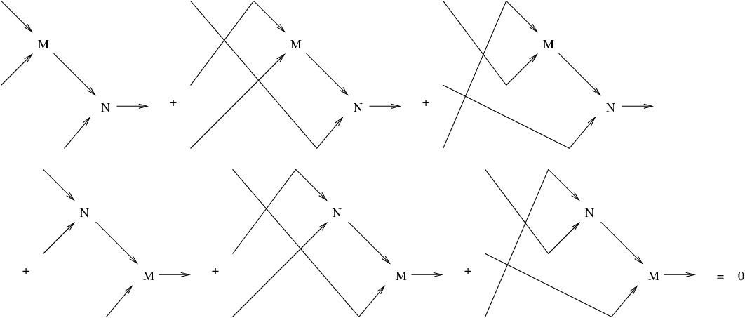
while the equations defining the variety of Lie algebra structures are shown in Figures 1 and 2.

By convention, the inputs for a picture are read anticlockwise starting from the output and the outputs are read clockwise starting from the input. (Since this is a confusing point, we remark that this convention makes sense only when our pictures have at least one input and output. Otherwise we will have to explicitly indicate which is the first input and which the first output of a picture.) Pictorial equations have translations in terms of structure constants and so the reader who is suspicious of pictorial arguments may translate everything into the language of structure constants.

In the variety of Lie algebra structures, those that are semisimple form an open set defined by the non-degeneracy of the Killing form. This symmetric form, denoted $B:V\otimes V\rightarrow{\mathbb{C}}$ is represented as in Figure 3.

To say that this form is non-degenerate implies the existence of an element $\theta\in V\otimes V$ (neccessarily unique and symmetric) satisfying the equation in Figure 4.

We recall here that the picture $\rightarrow$ represents the identity endomorphism of $V$. Also note that since $\theta$ is symmetric, it is unneccesary to specify the order of its outputs.

Since we wish to deal with varieties rather than open subsets of such, we consider the subvariety $X$ in $(V^{*}\otimes V^{*}\otimes V)\oplus(V\otimes V)$ with coordinate functions $\mu_{ij}^{k}$ and $\theta^{ij}$ defined by the equations in Figures 1, 2 and 4. It should be clear that points of $X$ are in bijective correspondence with semisimple Lie algebra structures on $V$ and that the $\mu_{ij}^{k}$ components of a point of $X$ determine - via the equation in Figure 4 - its $\theta^{ij}$ components.

The natural action of the group $G=GL(V)$ on $(V^{*}\otimes V^{*}\otimes V)\oplus(V\otimes V)$ restricts to an action on $X$ and the orbits correspond to isomorphism classes of $n$-dimensional complex semsimple Lie algebras. We assert that all $GL(V)$ orbits are open in $X$. While this is the well known rigidity of semisimple Lie algebras (see [Grs] or [NjnRch]), for completeness, we sketch a proof.

From the equations defining the variety $X$, it follows that the Zariski tangent space of $X$ at a point $(\mu,\theta)$ is contained in the solution space of the linear equations in $(\mu^{\prime},\theta^{\prime})$ given in Figures 5, 6 and 7.

We may use the equations in Figures 4 and 7 and the symmetry of $B$ and $\theta$ to “solve” for $\theta^{\prime}$ in terms of $\mu^{\prime},\mu$ and $\theta$ as in Figure 8.

Thus the Zariski tangent space is identified with a subspace of the solution space of the linear equations in Figures 5 and 6 in the variables $\mu^{\prime}$.

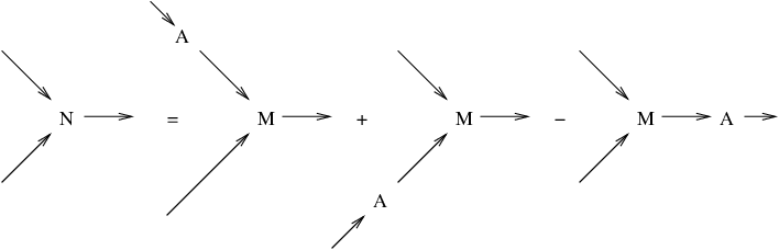
Some “obvious elements” in the tangent space are obtained from the $G$-action by pushing forward the Lie algebra ${\mathfrak{gl}}(V)$ of $G$ by the map induced by: $G\ni T\mapsto T.(\mu,\theta)\in X$. Explicitly, consider $A\in{\mathfrak{gl}}(V)$. The one-parameter subgroup $e^{At}$ acts on $(\mu,\theta)=(\mu_{0},\theta_{0})$ as illustrated in Figure 9.

Taking the derivative with respect to $t$ and evaluating at $t=0$ gives the pictorial equation in Figure 10

as an obvious solution to the equations in Figures 5 and 6.

Comparing with the complex below - see §7.2.1 of [GdmWll] -

that calculates the cohomology of the adjoint module ${\mathfrak{g}}$ over the Lie algebra ${\mathfrak{g}}$ corresponding to the point $(\mu,\theta)$ of $X$, we see that the equations in Figures 5 and 6 exactly translate to saying that $\mu^{\prime}$ is in $Hom(\wedge^{2}{\mathfrak{g}},{\mathfrak{g}})$ and is a cocycle in the complex while the obvious solutions are the coboundaries.

Since ${\mathfrak{g}}$ is semisimple, this cohomology vanishes - see Theorem 3.12.1 of [Vrd] - which may be interpreted to mean that the map $G\rightarrow X$ considered above is surjective at the tangent space level at the identity of $G$. Since this holds for each point in the orbit, a simple geometric argument - see Corollary 1.5 of [Stf] - shows that the orbit is Zariski open in $X$.

Hence there are only finitely many orbits each of which is also Zariski closed (and the variety $X$ is non-singular). We now appeal to what [MmfFgrKrw] refer to as the ‘only really important geometric property implied by the reductivity of $G$’ - see Corollary 1.2 of Chapter 1, §2 - any two orbits are separated by an element in $R^{G}$ where $R={\mathbb{C}}[\mu_{ij}^{k},\theta^{ij}]$ is the coordinate ring of the ambient space. It remains to describe this invariant subring explicitly. This is exactly what the main result of [DttKdySnd] does. According to that, a linear spanning set of the invariant ring is given by all “closed pictures” that can be formed using the two tensors $\mu$ and $\theta$. Further, from computational invariant theory - see §4.7 of [DrkKmp] - $R^{G}$ is generated as an algebra by its elements of degree at most $\frac{3}{8}(n^{3}+n^{2})(n+1)^{2}(2n+1)^{2n^{2}}$ - the numbers $n^{3}+n^{2}$, $n+1$, $2n+1$ and $n^{2}$ being upper bounds for what they call $r,C,A$ and $m$ respectively. Since any closed picture made up of $\mu$’s and $\theta$’s has twice as many $\mu$’s as $\theta$’s it follows that closed pictures involving at most $k(n)=\frac{1}{8}(n^{3}+n^{2})(n+1)^{2}(2n+1)^{2n^{2}}$ $\theta$’s separate isomorphism classes of complex semisimple Lie algebras of dimension $n$.

We will now analyse an arbitrary closed picture involving $\mu$’s and $\theta$’s and show that it can be reduced modulo the relations in Figures 1, 2 and 4 to linear combinations of products of chord diagrams. The interpretation of a chord diagram as a closed picture made out of the tensors $\mu$ and $\theta$ is most easily illustrated by an example as in Figure 11 below. Briefly,

put in a $\mu$ at each point of the circle determined by the chords, put in a $\theta$ on each of the chords and orient arrows as in the example.

Before proceeding with this proof, we pause to observe a useful pictorial consequence of the cyclic symmetry of the trilinear form: $a\otimes b\otimes c\mapsto B([a,b],c)$. This is the pictorial equality in Figure 12.

To prove this equation, use the non-degeneracy of $B$ to reduce to proving the equality in Figure 13. (The $*$’s are supposed to indicate which is the first input since these are pictures without outputs.)

But now, using the symmetry of $B$ and $\theta$ and the equation in Figure 4, we see that this is pictorial translation of the cyclic symmetry of the trilinear form above. What we will actually use is the corollary in Figure 14 of the equation in Figure 12, the easy proof of which is left to the reader.

Consider now an arbitrary closed picture, say $P$, involving $\mu$’s and $\theta$’s. We will first discuss the case that $P$ is connected. Suppose that the number of $\theta$’s in $P$ is $k$ so that the number of $\mu$’s is $2k$. Removing all $\theta$’s from the picture gives a picture, say $Q$, that specifies a map from $V^{\otimes 2k}$ to ${\mathbb{C}}$ (after choosing an order on its inputs) that is expressible using only $\mu$’s. While $Q$ is not neccessarily connected, note that in the equation in Figure 14, the picture on the right remains connected after removing $\theta$ while that on the left is disconnected. Thus by using this corollary as often as needed we may asume that $Q$ is connected.

Consider $Q$ as a connected directed graph where each vertex is either univalent with outdegree $1$ or trivalent with indegree $2$ and outdegree $1$. We claim that there is exactly one directed cycle in this graph. To see this, observe that $Q$ has $4k$ vertices - $2k$ of them trivalent and $2k$ univalent - and $4k$ edges - by counting valencies. So, regarded as an undirected graph, it has exactly one cycle. To see that this cycle is, in fact, directed, consider it as a subgraph of the original directed graph and look at the list of pairs $(i,o)$ where $i$ is the indegree and $o$ is the outdegree - in the cycle - of each vertex. Each pair is one of $(0,2),(2,0),(1,1)$ and the sum of the $i$’s is equal to the sum of the $o$’s. Hence the number of vertices in this cycle with data $(0,2)$ is equal to that with data $(2,0)$. Since each vertex is a $\mu$, it is not possible that $(0,2)$ occurs for any vertex and therefore each vertex is of type $(1,1)$. This means that the cycle is directed.

Next, note that by using the antisymmetry relation we may assume that for all the $\mu$’s occuring in the cycle, the in-edge of $\mu$ that is part of the cycle is the one corresponding to its second input. Thus we assume that $Q$ is of the form shown in Figure 15 where the $P_{i}$ are pictures

representing maps from some tensor power of $V$ to $V$ that are made up of $\mu$’s and do not have cycles.

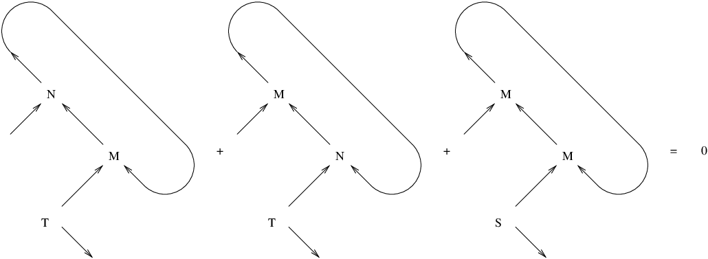
Next we will induce on the total number of $\mu$’s occuring in all the $P_{i}$ to show that we may reduce to the case that this number is $0$. This is easy and follows immediately from the Jacobi identity written in the form in Figure 16.

Basically, we may get rid of the complexity inside a circle at the expense of increasing its size.

We have therefore seen that modulo the relations in Figures 1, 2 and 4 any connected closed picture made up of the tensors $\mu$ and $\theta$ is equivalent to a linear combination of pictures associated to chord diagrams. In case the original picture is disconnected, we will have to allow for a linear combination of products of pictures associated to chord diagrams. A review of the proof shows that if the original picture involved $k$ $\theta$’s, then so do the resulting chord diagrams.

While a closed picture made up of $\theta$’s and $\mu$’s corresponds to an element in the polynomial ring $R={\mathbb{C}}[\mu_{ij}^{k},\theta^{ij}]$, recall that for a point lying on $X$, $\theta^{ij}$ may be expressed as a rational function of the $\mu_{ij}^{k}$ and thus each such closed picture - in particular, a chord diagram - determines a rational function in the $\mu_{ij}^{k}$ on $X$.

To summarise, we have proved the following theorem.

We conclude by observing that these numbers associated to a chord diagram and a complex semisimple Lie algebra are exactly those studied in [Brn] and are essentially equivalent to the weight systems associated to such a Lie algebra and its adjoint representation.

References

- [Brn] Dror Bar-Natan, On the Vassiliev knot invariants, Topology, 34, (1995), 423-472.
- [DrkKmp] H. Derksen and G. Kemper, Computational invariant theory, Encyc. of Math. Sc. 130, Springer-Verlag, 2002.
- [DttKdySnd] Sumanth Datt, Vijay Kodiyalam and V. S. Sunder, Complete invariants for complex semisimple Hopf algebras, Math. Res. Lett., 10, (2003) 571-586.
- [GdmWll] R. Goodman and N.R. Wallach, Representations and invariants of the classical groups, Encyc. of Math. and Its Appl. 68, Cambridge Univ. Press, 1998.
- [Grs] Murray Gerstenhaber, On the deformation of rings and algebras, Ann. of Math.(2), 79, (1964) 59-103.
- [KffRdf] L. H. Kauffman and D. E. Radford, On two proofs of the existence and uniqueness of integrals for finite-dimensional Hopf algebras, In New trends in Hopf algebra theory, Contemp. Math., 267, (2000) 177-194.
- [Kpr] G. Kuperberg, Non-involutory Hopf algebras and 3-manifold invariants, Duke. J. Math., 84, (1996) 83-129.
- [MmfFgrKrw] D. Mumford, J. Fogarty and F. Kirwan, Geometric Invariant theory, Third Edition, Ergebnisse der Mathematik und ihre Grenzgebiete 34, Springer Verlag, Berlin (1994).
- [NjnRch] A. Nijenhuis and R. W. Richardson, Cohomology and deformations in graded Lie algebras, Bull. Amer. Math. Soc., 72, (1966) 1-29.
- [Stf] D. Stefan, The set of types of -dimensional semisimple and cosemisimple Hopf algebras is finite, J. Alg., 193, (1997), 571-580.
- [Vrd] V. S. Varadarajan, Lie groups, Lie algebras and their representations, Graduate Texts in Mathematics 102, Springer Verlag, (2002).