The Kauffman bracket skein moduleof a twist knot exterior

At first glance, and in original intent [13], the Kauffman bracket skein module is a formal extension of the Kauffman bracket polynomial to an arbitrary 3-manifold. As Kauffman’s polynomial (for framed links in $S^{3}$) is equivalent to the Jones polynomial (for oriented links in $S^{3}$), one may think of the skein module as a generalization of the Jones polynomial. More recently the module has taken on a different significance: it is now seen as a deformation of the $SL_{2}(\mathbb{C})$-characters of the fundamental group [4, 5, 14]. Using this interpretation of the skein module of a knot exterior, Frohman, Gelca and the second author here constructed a quantum version the $A$-polynomial [6]. This is related back to the Jones polynomial [15, 16] (not simply by generality) and has implications for the hyperbolic volume conjecture [9, 12]. Despite all this, there have as yet been no computations of Kauffman bracket skein modules for hyperbolic manifolds.

Early computations [13] depended on an $I$-bundle structure for the manifold, since projection along the $I$ factor gave a natural mechanism for controlling complexity. The only other successful method [1, 7, 8] has been to consider the effect of adding a single 2-handle to a handlebody. This creates a presentation with fairly simple generators (any basis for the module of the handlebody), but having an unwieldy set of relations. Eliminating redundant relations is the most difficult part of the task. What is needed is an effective method of creating relations among relations, or syzygies, and then keeping track of which relations can be removed.

This has been managed for all genus one manifolds [7, 8], and for $(2,q)$-torus knot exteriors [1]. In principle, the combinatorics ought to be accessible for genus two manifolds with toral boundary (one added handle), but the computations are quite daunting in practice. Even for $(2,q)$-torus knots, the trick was managed only with help from a particularly nice basis.

The innovation in this paper is a simpler method of keeping track of the relations. We use the established handle addition technique, but we twist the handlebody instead of the handle, which simplifies many bracket computations. Our viewpoint also leads to a comfortable and practical method for producing syzygies that reduce the initial presentation to a simple basis.

Let $M$ be an orientable 3-manifold. A framed link in $M$ is an embedding of a disjoint collection of annuli into $M$. Framed links are depicted by link diagrams showing the cores of an annuli lying flat in the projection plane (i.e. with blackboard framing).

Two framed links in $M$ are equivalent if there is an isotopy of $M$ taking one to the other. Let $\mathcal{L}_{M}$ denote the set of equivalence classes of framed links in $M$, including the empty link. With $R=\mathbb{Z}[t^{\pm 1}]$, form a free module $R\mathcal{L}_{M}$ with basis $\mathcal{L}_{M}$. Define $S(M)$ to be the smallest submodule of $R\mathcal{L}_{M}$ containing all expressions of the form $\displaystyle{\raisebox{-5.0pt}{\mbox{}\hskip 1.0pt \psfig{file}\hskip 1.0pt\mbox{}}-t\raisebox{-5.0pt}{\mbox{}\hskip 1.0pt \psfig{file}\hskip 1.0pt\mbox{}}-t^{-1}\raisebox{-5.0pt}{\mbox{}\hskip 1.0pt \psfig{file}\hskip 1.0pt\mbox{}}}$ and $\bigcirc+t^{2}+t^{-2}$, where the framed links in each expression are identical outside balls pictured in the diagrams. The Kauffman bracket skein module $K(M)$ is the quotient

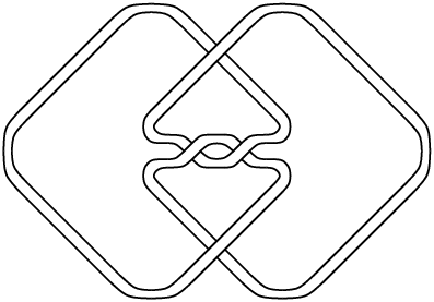
A $q$-twist knot (right-handed, if not amphichiral) is the alternating knot formed by inserting a left-to-right string of $q$ half-twists into the coupon in Figure 1. The 2-twist knot in Figure 2, for example, is the familiar figure-8 knot. Let $M_{q}$ be the twist knot exterior, and denote by $xy$ the 0-framed, two component link also pictured in Figure 1. The meridian is $x$ and the other component is $y$. In general, $x^{l}y^{m}$ denotes the cable of $xy$ consisting of $l$ parallel copies of $x$ and $m$ parallel copies of $y$. The exponents run over non-negative integers and 1 denotes the empty link.

The knot exterior $M_{q}$ decomposes into a pair of genus two handlebodies glued along the 4-punctured sphere $S$ shown in Figure 3. Let $H$ be the closure of the component of $M_{q}-S$ containing the coupon. Figure 4(a) depicts $H$, slightly deformed so that the upper left and lower right punctures are in the foreground.

The portions of the knot outside $H$ are parallel to a pair of arcs in $S$ that cut it into an annulus. Therefore, $M_{q}$ is homeomorphic to $H$ with a 2-handle attached along this annulus. Its core is shown in Figure 4(b).

There is a standard argument [1, 2, 7, 8, 10] that says $K(M_{q})$ is $K(H)$ modulo skeins differing by slides across the 2-handle. We find this language to be a little imprecise, so we will rephrase it in terms of relative skeins. Suppose that the core of the attaching annulus is given the blackboard framing in $S$. We cut out a very small bit of this curve, as indicated in Figure 4(c), leaving a framed arc whose ends are a pair of framed points in $\partial H$. Following [11, 13], let $K_{1}(H)$ be the skein module of $H$ relative to those two framed points.

Let $L$ be a relative link in $H$. Since the ends of $L$ are very close together we can unambiguously define the completion of $L$ to be the result of gluing its ends together. The slide of $L$ is formed by gluing its ends to the cut open core of the attaching annulus. Completion and slide are denoted by $c(L)$ and $s(L)$. Let $r(L)=c(L)-s(L)$ and extend linearly to $r\co K_{1}(H)\to K(H)$. The image of $r$ is the set of all possible relations in $K(H)$ induced by handle slides. Therefore,

Since $K(H)$ is free, the quotient provides a presentation of $K(M_{q})$. Any basis for $K(H)$ serves as a generating set. For relations, choose generators for $K_{1}(H)$, apply $r$, and express everything in terms of the basis of $K(H)$. The more efficient your generating set for $K_{1}(H)$, the more efficient your presentation. However, even a basis for $K_{1}(H)$ yields unnecessary relations. Computing $K(M_{q})$ thus becomes a search for all relations among the relations in this presentation.

We need to fix a basis for $K(H)$. Let $x$ and $y$ be the knots in Figure 1, but only up to isotopy in $H$. Let $z$ be a meridian that is not isotopic to $x$ in $H$. As usual, $x$, $y$ and $z$ are 0-framed. The set of cables, $\mathcal{B}=\{x^{l}y^{m}z^{n}\}$, is a basis for $K(H)$ [13].

We also need to fix generators of $K_{1}(H)$, but first some notes on multiplicative notation for (possibly relative) links in $H$.

• •

  The notation is commutative and associative.

• •

  $x^{l}$, $y^{m}$ and $z^{n}$ denote cables.

• •

  If $L$ is a (possibly relative) link then $x^{l}L$ means the union of $L$, pushed away from the knot boundary, with a cable of $x$ very near the knot boundary.

• •

  Similarly for $z^{n}L$.

• •

  If $\sigma$ is a (possibly relative) skein then $x^{l}z^{n}\sigma$ is defined by distributing $x^{l}z^{n}$ across any linear combination of links representing $\sigma$. This is well defined because representatives of $\sigma$ differ by skein relations that take place away from the knot boundary.

• •

  If $\sigma$ is written in terms of the basis $\{x^{i}y^{j}z^{k}\}$ then $x^{l}z^{n}\sigma$ is just polynomial multiplication.

• •

  In general, $y^{m}L$ is not well defined, but there are some specific embeddings of $L$ for which we want $y^{m}L$ to make sense. These are explained below.

If $L$ is one of the relative knots

$$X=\raisebox{-11.0pt}{\mbox{}\hskip 1.0pt \psfig{file,height} \hskip 1.0pt\mbox{}},\quad Z=\raisebox{-11.0pt}{\mbox{}\hskip 1.0pt \psfig{file,height} \hskip 1.0pt\mbox{}}\quad\text{or}\quad U=\raisebox{-11.0pt}{\mbox{}\hskip 1.0pt \psfig{file,height} \hskip 1.0pt\mbox{}}$$

then $y^{m}L$ denotes a copy of $y^{m}$ inserted into the twist coupon. If $0\leq k\leq q$, let

$$Y_{k}=\mbox{\raisebox{-16.0pt}{\mbox{}\hskip 1.0pt \psfig{file,height}} \hskip-70.0pt{\tiny{$q-k$}}\hskip 17.0pt {\tiny{$k$}}\hskip 22.0pt\mbox{}}$$

where the coupons contain $q-k$ and $k$ twists. By $y^{m}Y_{k}$ we mean a cable of $y$ inserted into the coupon containing $k$ twists, even if $k=0$. Lastly,

$$y^{m}Y_{-1}=\mbox{\raisebox{-16.0pt}{\mbox{}\hskip 1.0pt \psfig{file,height}} \hskip-63.0pt{\tiny{$q$}}\hskip 26.0pt {\tiny{$0$}}\hskip 22.0pt\mbox{}}$$

with $y^{m}$ inserted in the coupon that contains no twists.

In this section we locate in $r(K_{1}(H))$ sufficient relations to eliminate all but $\{x^{l}y^{m}\;|\;m\leq q\}$ from $\mathcal{B}$. It turns out that powers of $z$ are easy to eliminate and that powers of $y$ index the complexity of other computations. For this reason, we introduce the notation $\sigma\sim y^{m}$, meaning $\sigma=t^{\pm p}y^{m}$ modulo the span of $\{x^{i}y^{j}z^{k}\;|\;j<m\}$.

Where $x$ and $z$ are concerned, the relation submodule behaves like an ideal.

In practice, you compute a relation by grinding some $r(\sigma)$ down to a polynomial in $x$, $y$ and $z$. Lemma 4.1 then says that any formal multiple of that relation by $x^{i}z^{k}$ is another relation. For example, from the relation $r(y^{m}Z)$ we obtain a class of relations:

Relations (1) can be used to eliminate $\{x^{l}y^{m}z^{n}\;|\;n>0\}$ from the presentation of $K(M_{q})$. Powers of $y$ are more troublesome. To eliminate $\{x^{l}y^{m}\;|\;y>q\}$, we need some new relations.

Lemmas 4.2 and 4.3 imply $r(y^{m}Y_{q})\sim y^{q+m+1}$. Extended to include powers of $x$, there relations serve to eliminate any remaining terms of $\mathcal{B}$ with $y$-degree greater than $q$. Hence, with

To finish the proof of Theorem 1 we must find relations among the relations $r(K_{1}(H))$ sufficient to write them all in terms of $\mathcal{R}$. Such a relation among relations is called a syzygy.

Here we show that $\mathcal{R}$ generates $r(K_{1}(H))$. Recall that $\mathcal{R}$ contains relations of the form

We need to show that the span of $\mathcal{R}$, denoted $\langle\mathcal{R}\rangle$, contains all relations of the form

We have shown that $\langle\mathcal{R}\rangle=r(K_{1}(H))$, so $K(M_{q})$ must be presented as in Proposition 1.

References

- [1] D Bullock, The -skein module of the complement of a torus knot, J. Knot Theory Ramifications 4 (1995) 619–632 \MR1361084
- [2] D Bullock, On the Kauffman bracket skein module of surgery on a trefoil, Pacific J. Math. 178 (1997) 37–51 \MR1447403
- [3] D Bullock, A finite set of generators for the Kauffman bracket skein algebra, Math. Z. 231 (1999) 91–101 \MR1696758
- [4] D Bullock, Rings of -characters and the Kaufman bracket skein module, Comment. Math. Helv. 72 (1997) 521-542 \MR1600138
- [5] D Bullock, C Frohman, J Kania-Bartoszyńska, Understanding the Kaufman bracket skein module, J. Knot Theory Ramifications 8 (1999) 265–277 \MR1691437
- [6] C Frohman, R Gelca, W Lo Faro. The A-polynomial from the noncommutative viewpoint, Trans. Amer. Math. Soc. 354 (2001) 735–747 \MR1862565
- [7] J Hoste, J H Przytycki, The -skein module of lens spaces; a generalization of the Jones polynomial, J. Knot Theory Ramifications 2 (1993) 321–333 \MR1238877
- [8] J Hoste, J H Przytycki, The Kauffman bracket skein module of , Math Z. 220 (1995) 65–73 \MR1347158
- [9] R M Kashaev, The hyperbolic volume of knots from the quantum dilogarithm, Lett. Math. Phys. 39 (1997) 269–275 \MR1434238
- [10] W Lo Faro, A Mayer-Vietoris Theorem for the Kauffman bracket skein module, PhD thesis, Univ. of Iowa (1998)
- [11] W Lo Faro, A Mayer-Vietoris Theorem for the Kauffman bracket skein module, J. Knot Theory Ramifications 8 (1999) 721–729 \MR1708008
- [12] H Murakami, J Murakami, The colored Jones polynomials and the simplicial volume of a knot, Acta Math. 186 (2001) 85–104 \MR1828373
- [13] J H Przytycki, Skein modules of 3-manifolds, Bull. Pol. Acad. Sci. 39 (1991) 91–100 \MR1194712
- [14] J H Przytycki, A Sikora, On skein algebras and -character varieties, Topology 39 (2000) 115–148 \MR1710996
- [15] T Takata, The colored Jones polynomial and the -polynomial for twist knots, \arxivmath.GT/0401068
- [16] Y Yokota, From the Jones polynomial to the -polynomial of hyperbolic knots, Interdisciplinary Inform. Sci. 9 (2003) 11-21 \MR2023102
Received:\qua2 February 2004 Revised:\qua3 February 2005