An Efficient Geometric Integrator for Thermostatted Anti-/Ferromagnetic Models
Abstract
(Anti)-/ferromagnetic Heisenberg spin models arise from discretization of Landau-Lifshitz models in micromagnetic modelling. In many applications it is essential to study the behavior of the system at a fixed temperature. A formulation for thermostatted spin dynamics was given by Bulgac and Kusnetsov [5], which incorporates a complicated nonlinear dissipation/driving term while preserving spin length. It is essential to properly model this term in simulation, and simplified schemes give poor numerical performance, e.g. requiring an excessively small timestep for stable integration. In this paper we present an efficient, structure-preserving method for thermostatted spin dynamics.
Keywords: Heisenberg ferromagnet, micromagnetics, spin dynamics, Landau-Lifschitz equation, Gilbert damping, thermostats, constant temperature, domain walls, geometric integrator, reversible method
1 Introduction
In recent years geometric integrators have become ubiquitous for numerical treatment of differential equations. By a geometric integrator is meant a numerical method that preserves some known structure of the continuous flow. Geometric integrators are particularly important for long term simulations, as used in molecular sampling or celestial mechanics. In this paper we consider the application of geometric integration principles for the types of spin dynamics systems which arise frequently in modelling of ferromagnets and anti-ferromagnets. Efficient Lie-Poisson schemes for classical spin dynamics described by the Landau-Lifshitz (LL) equation were studied in [10], and related multisymplectic schemes in [9]. Here we develop and test a geometric integrator for a semi-discrete Landau-Lifshitz-Gilbert (LLG) equation which includes a nonlinear dissipative term. This dissipative system forms the foundation for a more complicated thermostatted model, following the approach of Bulgac and Kusnetsov [5, 2]. We design an effective splitting technique for the full coupled system.
LL and LLG are currently a very active topic of research. Other approaches to them can be found in [9, 23, 6, 10, 19, 21, 14, 17], who also provide further references. However none of these consider a thermostatted version.
Simulation with the thermostatted version shows fascinating global behavior: the system first arranges into patterns (spin domains) with slowly moving domain walls, then goes into a quasi-chaotic state and quickly rearranges itself into completely new spin domains. This kind of transition would not be possible with local interactions only. Here the thermostatting variable is defined in such a way that it has a global character.
A number of recent articles have focussed on the geometric integration of molecular systems in the canonical ensemble [4, 15, 3, 12]. In these articles, the aim has been to start from a Hamiltonian formulation for thermostatted molecular simulation and then to provide a suitable symplectic integrator. The starting point is usually Nosé dynamics, although generalizations are possible.
Since the constant energy Heisenberg spin system is Lie-Poisson, it is natural to seek a Lie-Poisson system to model the action of the thermostat. While it is possible (with some additional complication, due to the presence of constraints) to develop such a model for the thermostatted Heisenberg model, based on the ideas in [12], it is much different in character from the corresponding molecular dynamics models (see the appendix). In particular, this approach appears to require introduction of many thermostatting variables which act differently on each spin vector of the system. In the context of magnetic models, this approach therefore sacrifices an important feature of Nosé molecular dynamics: the apparent compatibility between the thermostatted quasi-dynamics and the microcanonical dynamics. (Even though Nosé dynamics is typically only validated based on a phase-sampling correspondence, there is widespread agreement that the thermostatted dynamics is relevant for modelling dynamics of an appropriate extended system which is not too different in character from the microcanonical version.) Moreover, the Lie-Poisson thermostats add additional complexity in the form of a relatively complex bath model.
Given these complications, we believe the best available starting point for geometric integration of thermostatted spin dynamics is the alternative framework of Bulgac and Kusnetsov, based loosely on Nosé-Hoover (NH) dynamics. Like NH molecular dynamics, these formulations sacrifice Hamiltonian structure, while retaining a reversing symmetry. It is unclear the extent to which this loss of structure affects the stability of methods and the ultimate resolution of macroscopic features of the spin model. Although in molecular dynamics it is known that the reversible-only methods are often inferior to their symplectic counterparts [13], it is also well established that NH-type methods are far superior to methods that are neither symplectic nor reversible.
The rest of the paper is organized as follows: in Section 1.1 we review splitting methods and apply them to our models. In Sections 2-4 we present the models and methods in detail. In Section 5 we present numerical results. Finally in Section 6 we present some conclusions and discussion.
1.1 Background: Review of splitting methods
The reader is referred to [16, 18] for a detailed discussion of splitting methods. To briefly describe their basic construction, consider a differential equation , with flow map . If , we have . If the flows on vector fields , , and share a first integral, then the composed map will preserve it as well. In this way, geometric integrators can be developed to preserve general classes of Lie groups. If the vector field is time-reversible, i.e. for some linear involution , then the symmetric concatenation or “Strang Splitting” , where , are reversible vector fields, gives a time-reversible map (), which, moreover, provides a second-order approximation of the solution on a finite time interval. As an example, if , the leapfrog (Störmer/Verlet) integrator results from the concatenation
The construction of splitting methods for various types of flows, and with various orders of accuracy, is discussed in a number of papers (see, e.g, [24, 20]). Practical splitting-based geometric integrators have been constructed by mathematicians, chemists and physicists for a wide variety of important applications, including the rigid body, general holonomic constraints, particle accelerator models, and the solar system. Vector field splittings were used in [10] to obtain efficient time-reversible integrators for (undamped) spin systems; it is this fundamental scheme that we have extended in this paper to treatment of dissipative and thermostatted systems.
2 The original Landau-Lifshitz model as a Poisson system
There are several versions of the Landau-Lifshitz equation depending on which forces and fields are taken into account. The version we use here is that of [7], discarding the external and demagnetizing field. (Schemes for more general formulations would build on the work presented here.) The equation can be written in the form:
| (1) |
where , an interval, is a unit vector in representing the classical spin at position and time , and is a diagonal matrix representing anisotropy. Clearly constant in time:
Following the usual practice, we discretize the spatial variable using second order central differences on a regular lattice as in [10] so that in the discretized system the unit length property is conserved. We then get a Poisson system on a lattice. Without loss of generality we may assume the lattice size to be :
hence (1) becomes
| (2) |
Note that the term can be dropped out. Here we have an lattice of spins: the variable is on the unit sphere of when . When either or index is zero or , those represent boundaries. Except for the case of periodic boundary conditions, these boundary terms are different from the spins: they are an artefact of discretization, and do not have a counterpart in the continuum case (1). Especially, they are not necessarily of unit length. We do not represent equations of motion to them, hence they are assumed constants.
By periodic boundary conditions we mean
| (3) |
Next we define the Poisson structure matrix. Let us denote
i.e. is a column vector. For an arbitrary we denote
The Poisson structure matrix is defined as the block diagonal
| (4) |
Now (2) becomes
when we choose the Hamiltonian
| (5) |
where NN refers to “nearest neighbours”:
and represents the boundaries. For example, if we have zero boundaries (), then
while if we have periodic boundary conditions, then
| (6) |
We can easily extend this to a model covering both ferromagnet and antiferromagnet case.
| (7) |
where is the so called exchange integral [1], assumed constant here, as in [2], and
Hence we have the Poisson system:
| (8) |
For an individual spin at the lattice point this becomes
| (9) |
in both periodic and non-periodic cases. From now on we employ the notation
Lemma 2.1.
Any system of the form with (4) and an arbitrary vector function, conserves the spin lengths in time:
| (10) |
Proof.
∎
This gives us useful freedom in modelling. Next, the anisotropy term is approximated by an average:
| (11) |
this is sometimes referred to [10] as the Roberts discretization. Now (9) becomes
| (12) |
where is a diagonal matrix and is modified according to (11).
Numerical method
As we noted above, (8) is a Lie-Poisson system whose meaning we recall here: we can define
which fulfills the Jacobi identity
hence is a Poisson bracket and is a Poisson structure matrix. Since is linear with respect to , this Poisson structure can be derived from a Lie algebra structure, hence it is called a Lie-Poisson structure.
For a detailed discussion on how to integrate this, see [10]. To summarize that paper, the best way to integrate is to split the vector field in even-odd (or red-black) way:
| (13) |
where
Now, both of these flows can be explicitly solved. For example : for odd . For even, the sum over includes only pairs with odd, hence they are constants (during ). Likewise in the sum is a constant. Denote the integrator of by and that of by . That is,
The implemented integrator is a symmetric composition of these exact flows:
| (14) |
This integrator
- •
is time reversible
- •
conserves spin lengths
- •
in isotropic case () preserves energy
since and do. See also Section 1.1.
3 Dissipated version
It is customary to add a dissipation term to (1). In our case the corresponding dissipated version is derived from (12) and becomes
| (15) |
where is a dissipation constant and the corresponding term is known as the Gilbert damping term.
Clearly (15) can be written more compactly
| (16) |
From lemma 2.1 it follows that everywhere, i.e. the dissipation does not affect spin lengths. Let us first look at the Gilbert damping term more closely through the equation
| (17) |
where , and and are constants. Or, more compactly,
This can be explicitly solved. Put
then (17) is
| (18) | |||||
| (19) | |||||
| (20) |
where constant,
We can solve for (we have assumed ):
| (21) |
where
Note: if , then
Substituting we can solve for , which is a scalar function times a constant vector:
Substituting we can solve for :
| (22) | |||||
| (23) |
where
| (24) | |||||
| (25) |
Note that the exp above is a matrix exponential, while the sin and cos are the usual scalar functions. Here is expanded as a Magnus series [11]: the direction of is constant, hence commutes with its integrals and Magnus series truncates after the first term. The evaluation of that term is by Rodriguez’ formula, hence (23).
Evaluating numerically was a problem because eventually approaches (physically this means becomes (anti-)parallel to ) so the in becomes zero. itself is not singular, however this presentation is difficult to evaluate. We used the following Taylor expansions in the implementation: if ,
and if ,
A Lyapunov function
Note that
hence
So is a Lyapunov function, when is positive. If , constant scalar, then
| (26) |
that is, is a lyapunov function iff sgn. Later sgn chooses between ferromagnet and antiferromagnet.
Several spins
Now we continue from (15), which can be written
| (27) |
Recall from the previous discussion that implies tends to become parallel to
This means, see (26), that if , then sgn and energy is decreasing. In other words, for a ferromagnet negative means energy damping.
To summarize, a ferromagnetic or antiferromagnetic spin system subject to Gilbert damping will uniformly dissipate energy for appropriate choice of the sign of the damping coefficient. Moreover, a Gilbert-damped system is spin-length conserving.
Numerical method
To integrate, we split the vector field in even-odd way as in the conservative case (Section 2)
| (28) |
where
Now, all these flows can be explicitly solved. For example : for odd . For even, the sum over includes only pairs with odd, hence they are constants (during ). Likewise in , , and the sums include only constants.
Hence in and we solve
| (29) |
and in and we solve
| (30) |
which are solved above. Note that (29), (30) have different ’s. The implemented integrator is a symmetric composition of these exact flows:
| (31) |
where are the exact flows.
An important feature of our method is that it dissipates energy when the flow (15) does. This can be seen in the following way: we solve the flows exactly, hence every step in the composition (31) follows the energy of the associated vector field exactly. Now is a second order method and it follows the energy evolution with accuracy . With small enough time step the error is negligible and our method dissipates the energy.
4 Thermostatted version
The motivation behind using thermostats is keeping the system around some constant average temperature. This is a reasonable assumption for example in systems with heat baths. That is, we allow the energy to fluctuate. But, at the same time, we want to keep the spin lengths constant. This will be carried out by modifying the dissipation term introduced in previous sections.
We use the thermostatting term suggested in [2]: choose a parameter (temperature) and compare the system’s energy to it, allow the damping coefficient to vary with time: and
| (32) |
where is temperature, and is Boltzmann’s constant which we hereafter take to be 1. is number of degrees of freedom, that is since we have an square lattice, is coupling strength and typically . Here we take . is equal to:
| (33) |
The thermostatting variable has been given the nickname “global demon” [2], so called due to its non-local (hence non-physical) character: it affects all spins simultaneously.
So our thermostatted system is
| (34) | |||||
| (35) |
It is possible to show that the ferromagnetic system thermostatted using (34),(35) samples from the canonical ensemble. This system also conserves spin length. Finally, one easily demonstrates that these equations are invariant under the simultaneous time-coordinate transformation , , , i.e. the equations are time-reversible.
Numerical method
To integrate, we split the vector field in even-odd way as above, with the term:
| (36) |
where as in Section 3 (with constant) and
| (37) |
Here we have simplified:
In all terms are constant so the equation with is trivially solved. But note that the update step of is .
| (38) |
where are the exact flows.
An important feature of this discretization is that it is time-reversible with respect to the mapping . This can be seen by recalling from Section 1.1 that if for some linear involution , then the Strang splitting gives a time-reversible map. Here and . Applying the rule four times in a row: first to and in the roles of and of Section 1.1, secondly to and in a similar way, next to and and finally to and , we get the claim.
5 Numerical results
In all our simulations we used , that is, a lattice. We used ferromagnets with anisotropy: diag. This is known as “easy plane” or “easy axis” anisotropy, corresponding to or , respectively.
5.1 Dissipated system
Example 1. In Figure 1 we see evidence of the dissipation of energy. On the top part is energy in semilog scale, on the bottom part is the maximum norm of the discrete Laplacian during each time step. Here we used periodic boundary conditions, , , and timestep . The initial configuration was random (top left of Figure 2).
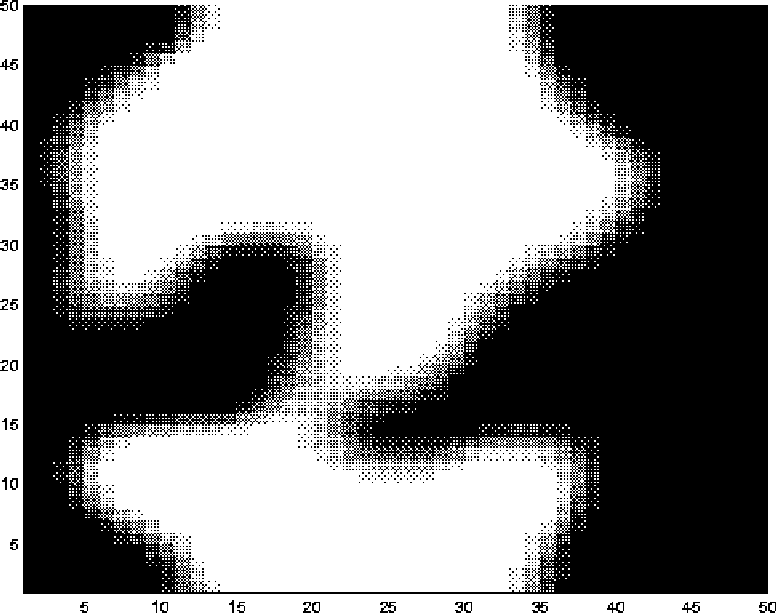
The evolution of the discrete Laplacian is understood as the system settling down to some formation, and this can be seen in Figure 2, which includes snapshots of the same simulation. The snapshots describe the components of the spins. The order of the pictures is top row first, from left to right. The darker a point is, the lower component it has. Black represents spin down, white spin up.
The result is typical: the dissipated system converges to two bands of up and down spins. We also tested zero boundary conditions, then the dissipated system typically converged to a single band.

 |
 |
 |
 |
 |
 |
5.2 Thermostatted system
Example 2. In Figures 3 and 4 is a thermostatted system with periodic boundaries, , and timestep . The initial condition is random. In the top part of Figure 3 is the thermostatting variable and in the middle part is the energy, and in the bottom part the maximum norm of the discrete Laplacian. After an initial phase both and energy settle to an aperiodic oscillatory motion, between and , energy between and . We plotted only 2000 steps but the behavior continued similarly for at least 25000 steps. In Figure 4 we can see slowly creeping boundaries; the reader is asked to compare the white areas. At it suddenly looks chaotic, then renders back to the creeping boundaries. This can be seen as a kind of stability of the creeping boundaries. After 25000 steps there still is slow motion, the system does not converge to any particular formation.

|
 |
 |
 |
 |
 |
Example 3. Another example, in Figures 5-8 is a thermostatted system we call “wandering vortices”. This beautiful system has random initial conditions, periodic boundaries, and parameters , and timestep . Figures 5 and 6 represent the evolution of , energy, and averages of the energy over different time windows. Interestingly, the behavior of is much wilder than in the Example 2. The snapshots in Figures 7,8 show the components of the lattice. From random state, the system very quickly forms vortices on smooth surrounding, which move around for a short time, then look random again, then vortices again. Sometimes the vortices died out completely leaving us just with smooth surface, then reappeared again.


 |
 |
 |
 |
 |
 |
 |
 |
 |
 |
 |
 |
 |
 |
 |
 |
 |
 |
Comparison to RK4 with projection
For comparison we implemented the classical Runge-Kutta order method (RK4) with projection: after every step we normalize
where denotes the result of RK4 step. At very small timesteps for which the RK4 method could successfully integrate the problem, it was slightly faster than splitting, but the RK4 method became rapidly unstable as the stepsize and/or anisotropy were increased. The splitting method was able to handle large anisotropies () and step sizes (). However, we did not seek the limits of our splitting method. The values and indicate the superior stability well enough at this stage.
We tested this projected RK4 on Examples 2 and 3. We kept the other parameters intact but changed the step size. As a sign of failure, we stopped the computation when the code started to produce infinities. In Example 2 the maximal timestep was 0.01, while in Example 3 . The results are summarized in table 1.
| Example 2 | RK4 survived until | |
| 0.020 | 0.060 | |
| 0.015 | 0.075 | |
| 0.012 | 0.084 | |
| 0.011 | 0.099 | |
| 0.0105 | 0.116 | |
| 0.0102 | 0.235 | |
| 0.010 | ||
| Example 3 | RK4 survived until | |
| 0.020 | 0.080 | |
| 0.019 | 0.095 | |
| 0.017 | 0.102 | |
| 0.016 | 0.112 | |
| 0.015 |
6 Discussion
In this paper we have developed and tested a geometric integrator for a semi-discretized Landau-Lifshitz-Gilbert (LLG) equation which includes a nonlinear dissipative term, as well as for a more complicated thermostatted model, following the approach of Bulgac and Kusnetsov.
The integrator for the dissipated system is shown to have a dissipative property. However, it is difficult to compare since we do not know the exact continuous solution. LLG is currently a very active topic of research, see more details in the introduction. However, it seems that so far there has not been developed a geometric integrator for a thermostatted system.
Trying to simulate the thermostatted systems with projected RK4 revealed both the features of a stiff ODE and features of a conservative system. The combination is extremely difficult for standard form numerical methods. The key feature of our splitting method is that it is constructed from composition of building blocks that simulate each of the two components of the system correctly.
Simulation with our new thermostatted method has revealed interesting phenomena: slowly creeping boundaries, or wandering vortices, both of which appear from random initial conditions. Our informal term “wandering vortices” in Example 3 refers not to certain particular vortices that survive throughout the whole simulation, but to a situation where we have two or more vortices which wander for a while, then violently crash and form new vortices. Intermediate states include “quasi-chaotic” state, an informal term by which we mean a state that suddenly appears and looks random but is not, since it renders immediately back to (almost) the same smooth motion.
The RK4 method is less stable. The stepsize restriction is an order of magnitude smaller compared to our splitting method. This is evidence of stiffness in the ODEs, and a better choice might seem to be a stiff solver on this account, but if one uses a stiff solver the result would be poor resolution of the conservative evolution which is also an important component of the dynamics of the system. The best compromise is therefore a composition scheme, such as that outlined here, which separately and appropriately resolves each term of the system.
We anticipate that this work will stimulate further research in the development of thermostatted numerical methods for systems with complicated nonlinear structure.”
Acknowledgement. The authors are grateful to Jason Frank both for valuable comments and providing the code of [10]. The author TA was supported by the Academy of Finland. BL was supported by the Engineering and Physical Sciences Research Council, grant GR/R03259/01.
References
- [1] J.C. Anderson. Magnetism and Magnetic Materials. Chapman and Hall, 1968.
- [2] V.P. Antropov, M.I. Katsnelson, B.N. Harmon, M. van Schilfgaarde, and D. Kusnezov. Spin dynamics in magnets: equation of motion and finite temperature effects. Phys. Rev. B, 54(2):1019–1035, 1996.
- [3] E. Barth, B. Laird, and B. Leimkuhler. Generating generalized distributions from dynamical simulation. J. Chem. Phys., 118, 5759-5768, 2003.
- [4] S. Bond, B. Laird, and B. Leimkuhler. The Nose-Poincare method for constant temperature molecular dynamics. J. Comput. Phys., 151, 114-134, 1999.
- [5] A. Bulgac and D. Kusnezov. Canonical ensemble averages from pseudomicrocanonical dynamics. Phys. Rev. A, 42(8):5045–5048, 1990.
- [6] W. E and X.-P. Wang. Numerical methods for the Landau-Lifshitz equation. SIAM J. Num. Anal., 38(5):1647–1665, 2000.
- [7] L.D. Faddeev and L.A. Takhtajan. Hamiltonian Methods in the Theory of Solitons. Springer Series in Soviet Mathematics. Springer, 1987.
- [8] X. Feng and P.B. Visscher. Stability and accuracy of Euler and quaternion micromagnetic algorithms. J. Appl. Phys., 91(10):8712–8714, 2002.
- [9] J. Frank. Geometric space-time integration of ferromagnetic materials. Technical report, CWI, Amsterdam, the Netherlands, October 2003.
- [10] J. Frank, W. Huang, and B. Leimkuhler. Geometric integrators for classical spin systems. J. Computat. Phys., 133, 1997.
- [11] E. Hairer, C. Lubich, and G. Wanner. Geometric Numerical Integration, volume 31 of Springer Series in Computational Mathematics. Springer, 2002.
- [12] B. Laird and B. Leimkuhler. Generalized dynamical thermostatting technique. Phys. Rev. E, 68, art. 016704, 2003.
- [13] B. Laird and J. Sturgeon. Symplectic algorithm for constant-pressure molecular-dynamics using a Nose-Poincare thermostat. J. Chem. Phys. 112 , 3474–3482, 2000.
- [14] D.P. Landau, A. Bunker, H.G. Evertz, M. Krech, and S.-H. Tsai. Spin dynamics simulations – a powerful method for the study of critical dynamics. arXiv:cond–mat 9912375, Center for Simul. Phys., Univ. Georgia, USA, Dec 1999.
- [15] B. Leimkuhler. A separated form of Nosé dynamics for constant temperature and pressure simulation. Comput. Phys. Comm., 148, 206-213, 2002.
- [16] B. Leimkuhler and S. Reich. Geometric Integrators in Hamiltonian Mechanics. Cambridge University Press, 2004.
- [17] D. Lewis and N. Nigam. Geometric integration on spheres and some interesting applications. J. Comp. Appl. Math., 151:141–170, 2003.
- [18] R. McLachlan and R. Quispel. Splitting methods. Acta Numerica, 11:341–434, 2002.
- [19] A. Prohl. Computational Micromagnetism. Adv. Numer. Math. Teubner, Stuttgart, 2001.
- [20] J. M. Sanz-Serna and M. P. Calvo. Numerical Hamiltonian Problems. Chapman & Hall, 1994.
- [21] M. Slodička and I. Cimrák. Numerical study of nonlinear ferromagnetic materials. Appl. Numer. Math., 46:95–111, 2003.
- [22] P.B. Visscher and X. Feng. Quaternion-based algorithm for micromagnetics. Phys. Rev. B, 65:104412, 2002.
- [23] X.-P. Wang, C.J. García-Cervera, and W. E. A Gauss-Seidel projection method for micromagnetics simulations. J. Computat. Phys., 171:357–372, 2001.
- [24] H. Yoshida. Construction of higher order symplectic integrators. Phys. Lett. A, 150(5–7):262–268, 1990.
Appendix: Lie-Poisson Canonical Sampling Technique
Consider first the Poisson rigid body system consisting of a Hamiltonian together with structure matrix admitting Casimir . Based partly on [12] we construct an augmented Hamiltonian with additional variables , , , :
where is an orthogonal matrix depending on parameter(s) . The Lie-Poisson structure is just the rigid body Poisson structure augmented by the canonical structure for the augmenting variables. Under assumption of ergodicity, and some very mild technical conditions similar to those obtained in [12], this Hamiltonian can be shown to provide canonical sampling from microcanonical trajectories i.e.
with preservation of the Casimir due to being orthogonal. In order to obtain ergodicity, the ”bath Hamiltonian” should be sufficiently complicated.
In the case of a spin system, , we may introduce a separate unit 3-vector for each spin vector. Then the Hamiltonian
will enable canonical sampling. For example can be a Householder transformation,
and the bath Hamiltonian can describe a coupled system of spherical pendula involving in some nontrivial way the parameter .