Matrix factorizations and link homology

The HOMFLY polynomial of oriented links in $\mathbb{R}^{3}$ is uniquely determined by the skein relation in figure 1 and its value on the unknot, see [HOMFLY].

The specialization $a=q^{n}$ and $b=q-q^{-1},$ for integer $n,$ produces a one-variable link polynomial which can be interpreted via representation theory of the quantum group $U_{q}(sl(n))$ if $n$ is positive, see [RT], $U_{q}(sl(-n))$ if $n$ is negative, and $U_{q}(gl(1|1))$ if $n=0,$ see [KS]. This polynomial is invariant under changing $q$ to $q^{-1}$ simultaneously with passing to the mirror image of the link; therefore, we don’t lose any information by restricting to non-negative $n.$ We denote this one-variable polynomial by $P_{n}(L),$ where $L$ is an oriented link; the normalization is

$$P_{n}(\mathrm{unknot})=[n]\stackrel{{\scriptstyle\mbox{\scriptsize{def}}}}{{=}}\frac{q^{n}-q^{-n}}{q-q^{-1}}$$

if $n>0,$ and $P_{0}(\mathrm{unknot})=1.$

For $n=0,1,2,3$ there exists a doubly-graded homology theory of links whose Euler characteristic is $P_{n}(L).$ Let us denote this theory by $H_{n}^{\prime}(L).$

• •

  $P_{0}(L)$ is the Alexander polynomial, and $H_{0}^{\prime}(L)$ was constructed by Peter Ozsváth and Zoltán Szabó [OS], and, independently, by Jacob Rasmussen [Ra]. Their theory exists in greater generality and, in particular, encompasses knots in homology spheres.

• •

  $P_{1}(L)=1$ and $H_{1}^{\prime}(L)\cong\mathbb{Z}$ for any oriented link $L,$ with $\mathbb{Z}$ in bidegree $(0,0).$ It will be clear subsequently that this is a natural choice for $H_{1}^{\prime}(L).$

• •

  $P_{2}(L)$ is the Jones polynomial; $H_{2}^{\prime}(L)$ was defined in [Kh1], and denoted by $\mathcal{H}(L)$ there. $H_{2}^{\prime}(\mathrm{unknot})$ is isomorphic to the integral cohomology ring of the 2-sphere.

• •

  $H_{3}^{\prime}(L)$ was constructed in [Kh3]. $H_{3}^{\prime}(\mathrm{unknot})$ is isomorphic to the integral cohomology ring of $\mathbb{CP}^{2}.$

The goal of the present paper is to construct, for each $n>0,$ a doubly-graded homology theory $H_{n}(L)$ with the Euler characteristic $P_{n}(L).$ The polynomial $P_{n}(L)$ can be computed by breaking up each crossing into a linear combination of diagrams of flat trivalent graphs, as in figure 2.

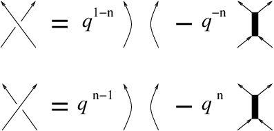
In these planar graphs some edges are oriented so that the neighbourhood of each unoriented edge (depicted by a thick line, and referred to from now on as a ”wide edge”) looks as on the rightmost pictures in figure 2. Two oriented edges ”enter” the wide edge at one vertex and two oriented edges ”leave” it the other. Of course, this arrangement could be used to provide each wide edge with a canonical orientation, but we won’t need it. In addition, oriented loops are allowed (an oriented loop is a crossingless plane projection of the oriented unknot).

There is a unique way to assign a Laurent polynomial $P_{n}(\Gamma)\in\mathbb{Z}[q,q^{-1}]$ to each such graph $\Gamma$ so as to satisfy all skein relations in figure 3.

In the representation theory language, an oriented edge stands for the vector representation $V$ of quantum $\mathfrak{sl}(n),$ and a wide edge for its (quantum) exterior power $\Lambda^{2}V.$ The trivalent vertex is the unique (up to scaling) intertwiner between $V^{\otimes 2}$ and $\Lambda^{2}V.$ The polynomial $P_{n}(\Gamma)$ has non-negative coefficients, see [MOY].

This calculus of planar graphs and its generalization to arbitrary exterior powers of $V$ was developed by Murakami, Ohtsuki and Yamada [MOY]. Oriented edges of graphs in their calculus carry labels from $1$ to $n-1$ that denote fundamental weights of $sl(n).$ The part of their calculus that we use deals only with edges labelled by $1$ and $2.$ In our notation we omit these labels; instead, we indicate edges labelled by $2$ by wide lines, see figure 4 top left. Consistency of figure 3 relations is shown in [MOY].

The last relation in figure 3 can be rewritten to introduce edges labelled by $3$ (see figure 4), and to say that the difference of certain two endomorphisms of $V^{\otimes 3}$ is a multiple of the projection onto the irreducible summand $\Lambda^{3}V.$

The polynomial invariant $P_{n}(L)$ of an oriented link $L$ can be computed by choosing a plane diagram $D$ of $L,$ resolving each crossing as shown in figure 2 and summing $P_{n}(\Gamma)$ weighted by powers of $q$ over all resolutions $\Gamma$ of $D:$

$$P_{n}(L)=P_{n}(D)\stackrel{{\scriptstyle\mbox{\scriptsize{def}}}}{{=}}\sum_{\mathrm{resolutions}\hskip 3.61371pt\Gamma}q^{\alpha(\Gamma)}P_{n}(\Gamma),$$

with $\alpha(\Gamma)$ determined by figure 2 rules. Independence from the choice of $D$ follows from the equations in figure 3. They imply that $P_{n}(D_{1})=P_{n}(D_{2})$ whenever $D_{1}$ and $D_{2}$ are related by a Reidemeister move.

To construct homology theory $H_{n},$ we first categorify $P_{n}(\Gamma),$ by defining in a rather roundabout way a graded $\mathbb{Q}$-vector space $H(\Gamma)={\mathop{\oplus}\limits_{j\in\mathbb{Z}}}H^{j}(\Gamma)$ such that

$$P_{n}(\Gamma)=\sum_{j\in\mathbb{Z}}\mathrm{dim}_{\mathbb{Q}}H^{j}(\Gamma)\hskip 3.61371ptq^{j}.$$

With $\Gamma$ we associate a 2-periodic complex $C(\Gamma)$ of graded $\mathbb{Q}$-vector spaces

$$C^{0}(\Gamma)\longrightarrow C^{1}(\Gamma)\longrightarrow C^{0}(\Gamma)$$

and define $H(\Gamma)$ as the degree $i$ cohomology of this complex, where $i$ is the parity of the number of components of link $L.$ The construction of $C(\Gamma)$ is based on the notion of a matrix factorization. An $(R,w)$-factorization $M$ over a commutative ring $R$ (where $w\in R$) consists of two free $R$-modules and two $R$-module maps

$$M^{0}\stackrel{{\scriptstyle d}}{{\longrightarrow}}M^{1}\stackrel{{\scriptstyle d}}{{\longrightarrow}}M^{0}$$

such that $d^{2}(m)=wm$ for any $m\in M.$ The most commonly considered case in the literature is when $R$ is the ring of power series, and $w$ satisfies a certain non-degeneracy assumption (that the quotient $R/(w)$ is an isolated singularity). Such $M$ is called a matrix factorization. When $w$ is homogeneous, one can switch from power series to polynomials.

Matrix factorizations appeared in commutative algebra in early and mid-eighties [E1], [B], [Kn], [S], [BEH] in the study of isolated hypersurface singularities, and much more recently in string theory, as boundary conditions for strings in Landau-Ginzburg models [KL1-3].

The tensor product $M\otimes_{R}N$ of an $(R,w)$-factorization $M$ and an $(R,-w)$-factorization $N$ is a 2-periodic complex of $R$-modules, with well-defined cohomology. More generally, given a finite set $\{w_{1},\dots,w_{m}\}$ of elements of $R$ that sum to zero, and an $(R,w_{i})$-factorization $M_{i},$ for each $i,$ the tensor product

$$M_{1}\otimes_{R}M_{2}\otimes\dots\otimes_{R}M_{m}$$

is a 2-periodic complex and its cohomology $H({\mathop{\otimes}\limits_{i}}M_{i})$ is a $\mathbb{Z}_{2}$-graded $R$-module.

Starting with a resolution $\Gamma$ of a link diagram, we denote by $E$ the set of oriented edges of $\Gamma$ and by $R$ the ring of polynomials in $x_{j},j\in E.$ We give each $x_{j}$ degree $2,$ making $R$ graded. Assume for simplicity that $\Gamma$ has no oriented loops and each wide edge of $\Gamma$ borders exactly four oriented edges (no oriented edge shares both endpoints with the same wide edge). Let $T$ be the set of wide edges. Choosing a $t\in T,$ denote the oriented edges at $t$ by $1,2,3,4$ (we think of $1,2,3,4$ as elements of $E$) so that the four corresponding variables are $x_{1},x_{2},x_{3},x_{4},$ see figure 5.

Assign the polynomial

$$w_{t}=x_{1}^{n+1}+x_{2}^{n+1}-x_{3}^{n+1}-x_{4}^{n+1}$$

to the edge $t.$ This polynomial lies in the ideal generated by $x_{1}+x_{2}-x_{3}-x_{4}$ and $x_{1}x_{2}-x_{3}x_{4}$ (since $x^{n+1}+y^{n+1}$ is a polynomial $g(x+y,xy)$ in $x+y$ and $xy$). Therefore, we can write

$$w_{t}=(x_{1}+x_{2}-x_{3}-x_{4})u_{1}+(x_{1}x_{2}-x_{3}x_{4})u_{2}$$

for some polynomials $u_{1},u_{2}.$ The latter are not uniquely defined, but the indeterminacy is easy to describe. We choose

	$\displaystyle u_{1}$	$\displaystyle=$	$\displaystyle\frac{x_{1}^{n+1}+x_{2}^{n+1}-g(x_{3}+x_{4},x_{1}x_{2})}{x_{1}+x_{2}-x_{3}-x_{4}},$
	$\displaystyle u_{2}$	$\displaystyle=$	$\displaystyle\frac{g(x_{3}+x_{4},x_{1}x_{2})-x_{3}^{n+1}-x_{4}^{n+1}}{x_{1}x_{2}-x_{3}x_{4}}.$

Let $C_{t}$ be the tensor product of factorizations

$$R\xrightarrow{x_{1}+x_{2}-x_{3}-x_{4}}R\stackrel{{\scriptstyle u_{1}}}{{\longrightarrow}}R$$

and

$$R\xrightarrow{x_{1}x_{2}-x_{3}x_{4}}R\stackrel{{\scriptstyle u_{2}}}{{\longrightarrow}}R.$$

$C_{t}$ is an $(R,w_{t})$-factorization. Define $C(\Gamma)$ to be the tensor product of $C_{t},$ over all wide edges $t,$

$$C(\Gamma)\stackrel{{\scriptstyle\mbox{\scriptsize{def}}}}{{=}}{\mathop{\otimes}\limits_{t\in T}}C_{t}.$$

The square of the differential in $C(\Gamma)$ is the sum of $w_{t},$ over all wide edges $t,$

$$d^{2}=\sum_{t}w_{t}=0.$$

The sum is $0,$ since for each oriented edge $i$ the term $x_{i}^{n+1}$ appears twice in the sum, once with positive and once with the negative sign. We see that $C(\Gamma)$ is a 2-periodic complex of $\mathbb{Q}$-vector spaces.

If, in addition, $\Gamma$ contains $k$ oriented loops, to define $C(\Gamma)$ we tensor the product of $C_{t}$’s with $k$ copies of the vector space $\mathrm{H}^{\ast}(\mathbb{CP}^{n-1},\mathbb{Q})$ and, if $k$ is odd, shift the complex. The shift $M\langle 1\rangle$ of a factorization $M^{0}\longrightarrow M^{1}\longrightarrow M^{0}$ is

$$M^{1}\longrightarrow M^{0}\longrightarrow M^{1}.$$

If, for some $t,$ some variables (say, $x_{2}$ and $x_{3}$) belong to the same oriented edge (see figure 6), we quotient the ring $R$ and the complex by the corresponding relation ($x_{2}=x_{3}$).

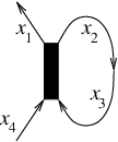
We let $H(\Gamma)$ be the cohomology of $C(\Gamma).$ The latter has cohomology only in degree equal to the parity of the number of components of link $L.$ Additional internal grading in $C(\Gamma)$ coming from the grading in the polynomial ring $R$ induces a $\mathbb{Z}$-grading on $H(\Gamma).$ This, in the nutshell, is how we define $H(\Gamma),$ which serve as building blocks for complexes $C(D)$ assigned to plane diagrams $D.$

In this paper we work in greater generality, first by allowing graphs that lie inside a disc and have points on its boundary. To such graph we assign a factorization, rather than a 2-periodic complex. Second, we place one or more marks on each oriented edge, with variables $x_{i}$ assigned to the marks, rather than just to the edges (see figure 7). Boundary points also count as marks. Let $E$ be the set of marks and $R$ the ring of polynomials in variables $x_{i},$ for $i\in E.$

To an arc bounded by marks $x_{i},x_{j}$ and oriented from $x_{j}$ to $x_{i}$ we assign the factorization $L^{i}_{j}:$

$$R\xrightarrow{\pi_{ij}}R\xrightarrow{x_{i}-x_{j}}R,$$

where

$$\pi_{ij}=\frac{x_{i}^{n+1}-x_{j}^{n+1}}{x_{i}-x_{j}}.$$

We then form the tensor product $C(\Gamma)$ of factorizations $C_{t},$ over all wide edges $t,$ and factorizations $L^{i}_{j},$ over all arcs. Now we ignore variables $x_{i}$ assigned to internal marks, and view $C(\Gamma)$ as an $(R^{\prime},w)$-factorization, with $R^{\prime}$ being the ring of polynomials in $x_{i},$ over all boundary points $i,$ and

$$w=\sum_{i}\pm x_{i}^{n+1},$$

with signs determined by the orientation of $\Gamma$ near boundary points. We prove that, in the homotopy category of factorizations, $C(\Gamma)$ does not depend on how we place internal marks.

For example, if $\Gamma$ is given in figure 7, to the wide edges $t_{1}$ and $t_{2}$ we assign polynomials $w_{t_{1}}$ and $w_{t_{2}}$ in variables $x_{1},x_{2},x_{3},x_{4}$ and $x_{5},x_{6},x_{8},x_{9},$ respectively, and factorizations $C_{t_{1}},C_{t_{2}}.$ Form the tensor product factorization

$$C(\Gamma)=C_{t_{1}}\otimes_{R}C_{t_{2}}\otimes_{R}L^{3}_{5}\otimes_{R}L^{7}_{6},$$

where $R$ is the ring of polynomials in $x_{1},\dots,x_{9}.$ We then ignore the variables $x_{3},x_{5},x_{6}$ that came from internal marks, and treat $C(\Gamma)$ as an $(R^{\prime},w)$-factorization with

$$w=x_{1}^{n+1}+x_{2}^{n+1}-x_{4}^{n+1}+x_{7}^{n+1}-x_{8}^{n+1}-x_{9}^{n+1},$$

and $R^{\prime}$ being the ring of polynomials in ”boundary” variables $x_{1},x_{2},$ $x_{4},x_{7},$ $x_{8},x_{9}.$ As an $R^{\prime}$-module, $C(\Gamma)$ is free but has infinite rank. However, by stripping off contractible summands, $C(\Gamma)$ can be reduced to a finite rank factorization.

We prove that factorizations $C(\Gamma)$ have direct sum decompositions that mimic skein relations in figure 3, and define homomorphisms $\chi_{0}$ and $\chi_{1}$ between factorizations $C(\Gamma^{0})$ and $C(\Gamma^{1})$ in figure 8.

Then we consider oriented tangles in a 3-ball $B^{3},$ such that all boundary points of a tangle lie on a fixed great circle of the boundary sphere. Let $D$ be a generic projection of tangle $L$ onto the plane of this great circle. We separate crossings of $D$ into positive and negative, following the rule in figure 45. To each crossing we assign two planar graphs (resolutions of this crossing), see figure 9.

To a diagram of a single crossing we assign the complex of factorizations

$$0\longrightarrow C(\Gamma^{0})\stackrel{{\scriptstyle\chi_{0}}}{{\longrightarrow}}C(\Gamma^{1})\longrightarrow 0$$

if the crossing is positive, and the complex

$$0\longrightarrow C(\Gamma^{1})\stackrel{{\scriptstyle\chi_{1}}}{{\longrightarrow}}C(\Gamma^{0})\longrightarrow 0$$

if the crossing is negative (shifts in the internal grading should be added to match powers of $q$ that appear in figure 2 formulas). In both cases we place $C(\Gamma^{0})$ in cohomological degree $0.$

In general, we place marks on each internal edge of $D,$ form a commutative cube of factorizations $C(\Gamma),$ over all resolutions $\Gamma$ of $D,$ and take the total complex $C(D)$ of the cube. Each factorization $C(\Gamma)$ has additional $\mathbb{Z}$-grading, induced by the grading of the polynomial ring $R,$ and the differential is grading-preserving. If we ignore the differentials, $C(\Gamma)$ is a $\mathbb{Z}\oplus\mathbb{Z}\oplus\mathbb{Z}_{2}$-graded $R$-module.

We prove that if $D_{1}$ and $D_{2}$ are related by a Reidemeister move, $C(D_{1})$ and $C(D_{2})$ are isomorphic as objects in a suitable homotopy category. Therefore, the isomorphism class of $C(D)$ in this category is an invariant of tangle $L.$

A cobordism $S$ between tangles $T_{0}$ and $T_{1}$ is an oriented surface properly embedded in $B^{3}\times[0,1]$ with $S\cap(B^{3}\times\{i\})=T_{i},$ and some additional standard assumptions. $S$ can be presented by a ”movie”–a sequence of plane diagrams of its cross-sections with $B^{3}\times k$ for various $k\in[0,1].$ The sequence starts with a diagram $D_{0}$ of $T_{0}$ and ends with a diagram $D_{1}$ of $T_{1}.$ To such a sequence we associate a homomorphism between complexes of factorizations $C(D_{0})$ and $C(D_{1})$ (with certain grading shifts thrown in), and show that, up to null-homotopies and multiplications by nonzero rationals, the homomorphism does not depend on the movie presentation of $S$ (as long as $D_{0}$ and $D_{1}$ are the first and the last slides). In this way, for each positive $n,$ we obtain an invariant of tangle cobordisms (trivial invariant if $n=1,$ and a variation of the one in [Kh4] if $n=2$).

If $L$ is a link, $C(\Gamma),$ for any resolution $\Gamma$ of $D,$ is a 2-periodic complex of graded $\mathbb{Q}$-vector spaces. It has cohomology groups only in degree equal to the parity of the number of components in $L.$ Thus, after removing contractible summands, $C(\Gamma)$ reduces to a graded vector space, and $C(D)$ to a complex of graded vector spaces. Its cohomology groups

$$H_{n}(D)={\mathop{\oplus}\limits_{i,j\in\mathbb{Z}}}H_{n}^{i,j}(D)$$

do not depend, up to isomorphism, on the choice of the projection of $L.$ The invariant of a link cobordism is a homomorphism between these cohomology groups, well-defined up to rescaling by nonzero rational numbers. Due to this, $H_{n}(D)$ are canonically (up to rescaling) associated to $L,$ rather than just to its diagram $D.$ Thus, notation $H_{n}(L)$ is justified. The Euler characteristic of $H_{n}(L)$ is the polynomial $P_{n}(L)$:

$$P_{n}(L)=\sum_{i,j\in\mathbb{Z}}(-1)^{i}q^{j}\dim_{\mathbb{Q}}H_{n}^{i,j}(L).$$

$H(\Gamma)$ is the cohomology of the complex $C(\Gamma)$ which has countable dimension as a $\mathbb{Q}$-vector space. However, since $H(\Gamma)$ is finite-dimensional, it’s nontrivial in finitely many degrees only, and an obvious upper bound on $|j|$ with $H^{j}(\Gamma)\not=0$ is $ne$ where $e$ is the number of edges in $\Gamma$ (both oriented and unoriented). The complex $C(D)$ is built out of finitely many $H(\Gamma),$ and the differential, being the signed sum of maps $\chi_{0},\chi_{1},$ can be determined combinatorially as well. Therefore, there exists a combinatorial algorithm to find homology groups $H_{n}(L),$ given $L.$

If $n=1,$ the factorization $C_{t}$ is contractible, and any graph with a wide edge has trivial homology. The homology of a circle is $\mathbb{Q}.$ This implies that $H_{1}(L)\cong\mathbb{Q},$ for any link $L,$ with $\mathbb{Q}$ in bidegree $(0,0).$

When $n=2$ and $\Gamma$ is closed (has no boundary points), its cohomology groups $H(\Gamma)$ are isomorphic to $A_{2}^{\otimes k},$ where $A_{2}$ is the cohomology ring of the 2-sphere and $k$ the number of circles in the diagram given by deleting all wide edges of $\Gamma.$ The equivalence of $H_{2}$ with a version of homology theory in [Kh1] follows easily from this observation. Specifically, for each link $L$ there is an isomorphism

$$H_{2}^{i,j}(L)\cong\mathcal{H}^{i,-j}(L^{!})\otimes_{\mathbb{Z}}\mathbb{Q},$$

where $L^{!}$ is the mirror image of $L,$ and $\mathcal{H}$ is the homology theory defined in [Kh1, Section 7] (programs computing $\mathcal{H}(L)$ were implemented by Dror Bar-Natan [BN1] and Alexander Shumakovitch [Sh]).

We conjecture that $H_{3}$ is isomorphic to the homology theory constructed in [Kh3], after the latter is tensored with $\mathbb{Q}.$ Both theories are doubly-graded, have the same Euler characteristic, and are built out of similar long exact sequences. The language of foams used in [Kh3] and [R] should extend from $n=3$ to all $n$ and lead to a better understanding of $H_{n}.$

Our categorification of polynomials $P_{n}(L)$ comes with several obvious caveats:

• •

  Homology groups $H_{n}(L)$ are finite-dimensional $\mathbb{Q}$-vector spaces rather than finitely-generated abelian groups (as in [Kh1], [Kh3] for $n=2,3.$)

• •

  Defining $H_{n}(L)$ requires a choice of a plane diagram. A more intrinsic definition would be most welcome.

• •

  Our invariants of link and tangle cobordisms are projective (defined up to overall multiplication by a non-zero rational number).

• •

  Reconstructing the Ozsváth-Szabó-Rasmussen theory (the $n=0$ case) using this approach would require additional ideas, lacking at the moment.

Construction of $C(\Gamma)$ involves tensoring factorizations

$$R\stackrel{{\scriptstyle a}}{{\longrightarrow}}R\stackrel{{\scriptstyle b}}{{\longrightarrow}}R$$

for various $a$’s and $b$’s. We do an elementary study of these tensor products in Section 2. Section 3 contains a review of matrix factorizations and their properties. In Section 4 we explain how to view factorizations as functors and present the identity functor via a factorization. These two sections also introduce general framework for diagrammatical interpretation of matrix factorizations. Section 5 treats graded factorizations and explains how to modify the material of previous sections to cover this case. Section 6 is the computational core of the paper. We define factorization $C(\Gamma)$ assigned to a planar graph $\Gamma,$ construct morphisms $\chi_{0},\chi_{1}$ between graphs $\Gamma^{0},\Gamma^{1}$ in figure 8, and prove direct sum decompositions of factorizations $C(\Gamma)$ that lift skein relations in figure 3. In Section 7 we associate a complex of factorizations $C(D)$ to a plane giagram $D$ of a tangle and state Theorem 2. This theorem, claiming the invariance of $C(D)$ under Reidemeister moves in a suitable category of complexes of factorizations, is proved in Section 8. In Section 9 we use matrix factorizations to construct 2-dimensional topological quantum field theories with corners. The next section deals with functoriality of our tangle invariant, extending it to tangle cobordisms. In the last section we briefly outline an approach to categorification of quantum invariants of links colored by arbitrary fundamental representations of $sl(n).$

Acknowledgments: M.K. is indebted to Ragnar-Olaf Buchweitz, Igor Burban, and Paul Seidel for introducing him to matrix factorizations, and to Igor Burban for sharing M.K.’s fascination with 2-periodic triangulated categories. L.R. would like to thank Anton Kapustin for explanations regarding topological 2-dimensional models and his work with Yi Li. We are grateful to Dror Bar-Natan and Greg Kuperberg for interesting discussions. While writing this paper we were partially supported by NSF grants DMS-0104139 and DMS-0196131.

Let $R$ be a Noetherian commutative ring. The Koszul complex $R(a_{1},\dots,a_{m})$ associated to a sequence $a_{1},\dots,a_{m},$ where $a_{i}\in R,$ is the tensor product (over $R$) of complexes

$$0\longrightarrow R\stackrel{{\scriptstyle a_{i}}}{{\longrightarrow}}R\longrightarrow 0$$

for $i=1,\dots,m.$ A sequence $(a_{1},\dots,a_{m})$ is called $R$-regular iff $a_{i}$ is not a zero divisor in the quotient ring $R/(a_{1},\dots,a_{i-1})R$ for each $i=1,\dots,m,$ and $R/(a_{1},\dots,a_{m})R\not=0.$ If the sequence is $R$-regular, its Koszul complex has cohomology in the rightmost degree only. For the converse to be true it suffices for $R$ to be local, see [E1, Section 17].

The Koszul complex can be written in a more intrinsic way. Let $N$ be a free $R$-module of rank $m$ and $a:R\to N$ an $R$-module homomorphism. The Koszul complex of $a$ is the complex of exterior powers of $N$:

$$0\longrightarrow R\longrightarrow N\longrightarrow\Lambda^{2}N\longrightarrow\Lambda^{3}N\longrightarrow\dots,$$

with the differential being the exterior product with $a(1)\in N.$ Choosing a basis of $N$ and writing $a(1)$ in the coordinates as $(a_{1},\dots,a_{m}),$ we recover the Koszul complex of this sequence.

In other words, $d^{2}m=wm$ for any $m\in M^{0}\oplus M^{1}.$ ”Duplex” is a term from [FKS], where it was used in a more general situation, with $R$ a (possibly noncommutative) ring and $w$ its central element.

A homomorphism $f:M\longrightarrow N$ of duplexes is a pair of homomorphisms $f^{0}:M^{0}\longrightarrow N^{0}$ and $f^{1}:M^{1}\longrightarrow N^{1}$ that make the diagram below commute.

$$\begin{CD}M^{0}@>{d^{0}}>{}>M^{1}@>{d^{1}}>{}>M^{0}\\ @V{f^{0}}V{}V@V{f^{1}}V{}V@V{f^{0}}V{}V\\ N^{0}@>{d^{0}}>{}>N^{1}@>{d^{1}}>{}>N^{0}\end{CD}$$

The category of $(R,w)$-duplexes and duplex homomorphisms is abelian.

A homotopy $h$ between homomorphisms $f,g:M\longrightarrow N$ of duplexes is a pair of maps $h^{i}:M^{i}\longrightarrow N^{i-1}$ (with indices understood modulo $2$) such that

$$f-g=hd_{M}+d_{N}h.$$

Null-homotopic morphisms constitute an ideal in the category of duplexes. We call the quotient category by this ideal the category of duplexes up to homotopies, or simply the homotopy category of duplexes. This category is triangulated. We denote the shift functor by $\langle 1\rangle.$

An $(R,0)$-duplex $M$ is equivalent to a 2-complex (periodic complex with period two) of $R$-modules. We denote the cohomology of an $(R,0)$-duplex $M$ by $H(M)\cong H^{0}(M)\oplus H^{1}(M).$

The homotopy category of $(R,w)$-factorizations is triangulated.

To a pair of elements $a,b\in R$ we associate an $(R,ab)$-factorization

$$R\stackrel{{\scriptstyle a}}{{\longrightarrow}}R\stackrel{{\scriptstyle b}}{{\longrightarrow}}R,$$

denoted $\{a,b\}.$

If $\mathbf{a}=(a_{1},\dots,a_{m})$ and $\mathbf{b}=(b_{1},\dots,b_{m})$ are two sequences of elements of $R,$ we consider the tensor product factorization $\{\mathbf{a},\mathbf{b}\}\stackrel{{\scriptstyle\mbox{\scriptsize{def}}}}{{=}}\otimes_{i}\{a_{i},b_{i}\},$ where the tensor product is over $R.$ We call $\{\mathbf{a},\mathbf{b}\}$ the Koszul factorization of the pair $(\mathbf{a},\mathbf{b}).$ We say that a pair $(\mathbf{a},\mathbf{b})$ is orthogonal if

$$\mathbf{a}\mathbf{b}\stackrel{{\scriptstyle\mbox{\scriptsize{def}}}}{{=}}\sum_{i}a_{i}b_{i}=0.$$

The tensor product $\{\mathbf{a},\mathbf{b}\}$ is a 2-complex iff $(\mathbf{a},\mathbf{b})$ is orthogonal, in which case we call it the periodic (or cyclic) Koszul complex of $(\mathbf{a},\mathbf{b}).$

Remark: We allow the case $m=0.$ Then $\mathbf{a}$ and $\mathbf{b}$ are empty sequences, $w=0,$ and the Koszul factorization is $R\longrightarrow 0\longrightarrow R.$

Remark: Factorizations $\{\mathbf{a},\mathbf{b}\}$ were defined in [BGS] and used there in the classification of finite CM-type singularities.

Proof: Write $1=\sum_{i}(a^{\prime}_{i}a_{i}+b^{\prime}_{i}b_{i}).$ The pair $(\mathbf{a}^{\prime},\mathbf{b}^{\prime}),$ where $\mathbf{a}^{\prime}=(a^{\prime}_{1},\dots,a^{\prime}_{m})$ and $\mathbf{b}=(b^{\prime}_{1},\dots,b^{\prime}_{m})$ defines a homotopy between the identity and the zero endomorphisms of $\{\mathbf{a},\mathbf{b}\}.$ $\square$

Let $I_{\mathbf{a},\mathbf{b}}\subset R$ be the ideal of $R$ generated by the entries of $\mathbf{a}$ and $\mathbf{b}.$

Proof: Multiplications by $a_{i}$ and $b_{i}$ are null-homotopic endomorphisms of $\{a_{i},b_{i}\},$ and, therefore, of $\{\mathbf{a},\mathbf{b}\}.$

$\square$

Let $\mathbf{a}^{i},\mathbf{b}^{i}$ be the sequences obtained from $\mathbf{a}$ and $\mathbf{b}$ by omitting $a_{i}$ and $b_{i},$ respectively. The factorization $\{\mathbf{a},\mathbf{b}\}$ is the ”total factorization” of the bifactorization

$$\{\mathbf{a}^{i},\mathbf{b}^{i}\}\stackrel{{\scriptstyle a_{i}}}{{\longrightarrow}}\{\mathbf{a}^{i},\mathbf{b}^{i}\}\stackrel{{\scriptstyle b_{i}}}{{\longrightarrow}}\{\mathbf{a}^{i},\mathbf{b}^{i}\}.$$

If $b_{i}$ is a nonzerodivisor in $R,$ the second map is injective (as map between $R$-modules), and the direct sum of the middle $\{\mathbf{a}^{i},\mathbf{b}^{i}\}$ and its image under the differential is contractible. Furthermore, suppose that $(\mathbf{a},\mathbf{b})$ is orthogonal. Then the quotient of $\{\mathbf{a},\mathbf{b}\}$ by this contractible subcomplex is isomorphic to $\{\mathbf{a}^{i},\mathbf{b}^{i}\}_{R^{\prime}},$ the periodic Koszul complex of the pair $(\mathbf{a}^{i},\mathbf{b}^{i})$ in the quotient ring $R^{\prime}\stackrel{{\scriptstyle\mbox{\scriptsize{def}}}}{{=}}R/(b_{i}).$ The quotient map induces an isomorphism on cohomology,

$$H(\{\mathbf{a},\mathbf{b}\})\cong H(\{\mathbf{a}^{i},\mathbf{b}^{i}\}_{R^{\prime}}),$$

the isomorphism is that of $R^{\prime}$-modules.

Likewise, if $a_{i}$ is a nonzerodivisor in $R$ and $(\mathbf{a},\mathbf{b})$ is orthogonal, the quotient map

$$\{\mathbf{a},\mathbf{b}\}\langle 1\rangle\longrightarrow\{\mathbf{a}^{i},\mathbf{b}^{i}\}_{R/(a_{i})}$$

induces an isomorphism on cohomology.

Motivated in part by Corollary 2, we introduce

If $(\mathbf{a},\mathbf{b})$ is homologically $R$-regular then $I_{\mathbf{a},\mathbf{b}}$ is a proper ideal in $R.$

Example: Let $m=1.$ An orthogonal pair $(a_{1},b_{1})$ is homologically $R$-regular iff $a_{1}R=\mathrm{Ann}(b_{1})$ and $b_{1}R$ is a proper subset of $\mathrm{Ann}(a_{1}).$ Furthermore, when $R$ is a domain, $(a_{1},b_{1})$ is homologically $R$-regular iff $a_{1}=0$ and $b_{1}$ is not invertible.

Example: Let ${\bf 0}=(0,\dots,0).$ The pair $({\bf 0},\mathbf{b})$ is homologically $R$-regular iff the Koszul complex of $\mathbf{b}$ has cohomology in the rightmost degree only.

Suppose there is a subset $J\subset\{1,\dots,m\}$ with even number of elements such that the sequence $(h_{1},\dots,h_{m})$ is $R$-regular, where $h_{i}=a_{i}$ if $i\in J$ and $h_{i}=b_{i}$ otherwise. Then $(\mathbf{a},\mathbf{b})$ is homologically $R$-regular and $H^{0}(\{\mathbf{a},\mathbf{b}\})\cong A/(h_{1},\dots,h_{m}).$

We can likewise define the notion of homologically $M$-regular pair $(\mathbf{a},\mathbf{b})$ for any $R$-module $M,$ and even for any $(R,w)$-duplex $M$. For the latter, we require $\mathbf{a}\mathbf{b}=-w,H^{0}(M\otimes_{R}\{\mathbf{a},\mathbf{b}\})\not=0$ and $H^{1}(M\otimes_{R}\{\mathbf{a},\mathbf{b}\})=0.$

Let $N$ be a finitely-generated free $R$-module and $\alpha:R\to N,\beta:N\to R$ be $R$-module maps. Consider the factorization $\{\alpha,\beta\}$ given by

$$\Lambda^{even}N\xrightarrow{\wedge\alpha+\neg\beta}\Lambda^{odd}N\xrightarrow{\wedge\alpha+\neg\beta}\Lambda^{even}N$$

(1)

where $\wedge\alpha$ is the wedge product with $\alpha(1),$

$$\wedge\alpha:\Lambda^{i}N\longrightarrow\Lambda^{i+1}N,$$

$\neg\beta$ is the contraction with $\beta,$

$$\neg\beta:\Lambda^{i}N\longrightarrow\Lambda^{i-1}N,$$

and

$$\Lambda^{even}N={\mathop{\oplus}\limits_{i}}\Lambda^{2i}N,\hskip 14.45377pt\Lambda^{odd}N={\mathop{\oplus}\limits_{i}}\Lambda^{2i+1}N.$$

$\{\alpha,\beta\}$ is a 2-complex iff $\beta\alpha=0,$ in which case we say that $\alpha$ and $\beta$ are orthogonal. Choosing a basis of $N$, we can write $\alpha=\mathbf{a}=(a_{1},\dots,a_{m})^{T}$ and $\beta=\mathbf{b}=(b_{1},\dots,b_{m}).$ Then $\{\alpha,\beta\}$ is isomorphic to $\{\mathbf{a},\mathbf{b}\}.$

Thus, with each element $\gamma\in N\oplus N^{\ast}$ we associate a factorization

$$\{\gamma\}\stackrel{{\scriptstyle\mbox{\scriptsize{def}}}}{{=}}\{\alpha,\beta\}$$

where $\gamma=\alpha+\beta$ and $\alpha\in N,\beta\in N^{\ast}.$

Suppose $g:N\to N$ is an automorphism of the $R$-module $N.$ Write the composition $\beta\alpha$ as $\beta\gamma^{-1}\gamma\alpha.$ The factorizations $\{\alpha,\beta\}$ and $\{\gamma\alpha,\beta\gamma^{-1}\}$ are isomorphic, and $GL(N,R)$ acts on the set of pairs $(\alpha,\beta)$ preserving isomorphism classes of factorizations $\{\alpha,\beta\}.$

We let the group $H=(\mathbb{Z}_{2})^{\times m}$ act on pairs by permuting $a_{i}$ with $a_{i}$ in $(a_{1},a_{1}),\dots,(a_{m},a_{m}),$ for $1\leq i\leq m.$

For $\sigma\in H,$ factorizations $\{\mathbf{a},\mathbf{b}\}$ and $\{\sigma(\mathbf{a},\mathbf{b})\}$ are isomorphic if $\sigma$ is an even permutation in $H\subset\mathbb{S}_{2m}.$ If $\sigma$ is odd, factorization $\{\sigma(\mathbf{a},\mathbf{b})\}$ is isomorphic to $\{\mathbf{a},\mathbf{b}\}\langle 1\rangle.$

The natural $R$-linear pairing between $N^{\ast}$ and $N$ induces a symmetric bilinear form on $N\oplus N^{\ast}.$ Let $G^{\prime}\subset GL(N\oplus N^{\ast},R)$ be the subgroup generated by $GL(N,R)$ and $H$ that act as described above. The action of $G^{\prime}$ preserves the inner product on $N\oplus N^{\ast}$ (with values in $R$). Let $G$ be the subgroup of $G^{\prime}$ that consists of all products $g_{1}\sigma_{1}\dots g_{r}\sigma_{r}$ of elements from $GL(N,R)$ and $H$ (over all $r$), such that $\sigma_{1}\dots\sigma_{r}$ is an even permutation.

The following result is clear.

The cyclic Koszul complex can be thought of as the square root of the Koszul complex. Namely,

$$\mathrm{Hom}_{R}(\{\mathbf{a},\mathbf{b}\},\{\mathbf{a},\mathbf{b}\})\cong\{\mathbf{a},\mathbf{b}\}\otimes_{R}\{-\mathbf{b},\mathbf{a}\}\cong R(\mathbf{a},\mathbf{b}),$$

where $R(\mathbf{a},\mathbf{b})$ is the Koszul complex of the length $2m$ sequence given by concatenating $\mathbf{a}$ and $\mathbf{b},$ with the grading collapsed from $\mathbb{Z}$ to $\mathbb{Z}_{2}.$

Potentials and their Jacobian algebras. Start with a finite set $x=\{x_{1},\dots,x_{k}\}$ of variables and let

$$R=\mathbb{Q}[[x]]\stackrel{{\scriptstyle\mbox{\scriptsize{def}}}}{{=}}\mathbb{Q}[[x_{1},\dots,x_{k}]]$$

be the algebra of power series in $x_{1},\dots,x_{k}$ with rational coefficients. Denote by $\mathfrak{m}$ the unique maximal ideal in $R$ (it’s generated by $x_{1},\dots,x_{k}$).

We say that a polynomial $w=w(x)\in\mathfrak{m}^{2}$ is a potential if the algebra $R/I_{w}$ is finite-dimensional, where $I_{w}\subset R$ is the ideal generated by partial derivatives $\partial_{i}w\stackrel{{\scriptstyle\mbox{\scriptsize{def}}}}{{=}}\partial_{x_{i}}w.$ Any polynomial $w\in R$ defines an algebraic map $\mathbb{C}^{n}\to\mathbb{C}.$ This map has an isolated singularity at $0$ iff $w$ is a potential.

A polynomial $w\in\mathfrak{m}^{2}$ is a potential iff $\partial_{1}w,\dots,\partial_{k}w$ is a regular sequence in $R,$ that is, $\partial_{i}w$ is not a zero divisor in $R/(\partial_{1}w,\dots,\partial_{i-1}w)R$ for each $1\leq i\leq k.$

The quotient algebra $R_{w}\stackrel{{\scriptstyle\mbox{\scriptsize{def}}}}{{=}}R/I_{w}$ is called the local algebra of the singularity and the Jacobian (or Milnor) algebra of $w.$ Its dimension is the Milnor number of the singularity.

A non-degenerate $\mathbb{C}$-linear trace $\mathrm{Tr}:R_{w}\otimes_{\mathbb{Q}}\mathbb{C}\to\mathbb{C}$ is given by the residue formula

$$\mathrm{Tr}(a)=\frac{1}{(2\pi i)^{k}}{{\mathop{\int}\limits_{|\partial_{j}w|=\epsilon}}}\frac{adx_{1}\dots dx_{k}}{\partial_{1}w\dots\partial_{k}w}$$

(2)

(this is proved in [GH, Chapter 5] and [AGV]). Therefore, the $\mathbb{C}$-algebra $R_{w}\otimes_{\mathbb{Q}}\mathbb{C}$ is symmetric. From [NN,Theorem 5] we deduce that $R_{w}$ is a symmetric $\mathbb{Q}$-algebra. $\square$

Exterior sum of potentials. Let $x$ and $y$ be two disjoint finite sets of variables. Define the exterior sum of potentials $w_{1}(x)$ and $w_{2}(y)$ as the potential $w_{1}(x)+w_{2}(y)$ in variables $x$ and $y.$ The Jacobian algebra of the exterior sum of potentials is the tensor product of Jacobian algebras: