Distribution of the Error in Estimated Numbers of Fixed Points of the Discrete Logarithm

Paragraph F9 of [6] includes the following problem, attributed to Brizolis: given a prime $p>3$, is there always a pair $(g,h)$ such that $g$ is a primitive root of $p$, $1\leq h\leq p-1$, and

In other words, is there always a primitive root $g$ such that the discrete logarithm $\log_{g}$ has a fixed point? This question has now been settled affirmatively by Campbell and Pomerance in [2]. The answer relies on an estimate for the number $N(p)$ of pairs $(g,h)$ which satisfy the equation, have $g$ is primitive root, and also have $h$ a primitive root which thus must be relatively prime to $p-1$. This result seems to have been discovered and proved by Zhang in [10] and later, independently, by Cobeli and Zaharescu in [3].

In [8] and [7], Pieter Moree and this author applied the same methods to estimate the number of solutions to (1) given no conditions on $g$ and $h$. Unfortunately, the error term involved in this estimate was completely unsatisfactory. It was also shown in [7] that for a positive proportion of primes a better error estimate can be obtained, and it was conjectured that one could do even better. The object of this note is to collect and analyze some data on the distribution of the actual error in these estimates.

The idea of repeatedly applying the function $x\mapsto g^{x}\bmod{p}$ is used in the famous cryptographically secure pseudorandom bit generator of Blum and Micali. ([1]; see also [9] and [5], among others, for further developments.) If one could predict that a pseudorandom generator was going to fall into a fixed point or cycle of small length, this would obviously be detrimental to cryptographic security. We hope that the investigation of the cycle structure of the discrete logarithm will therefore eventually be of some use to those interested in the field of cryptography.

Using the same notation as in the previously cited papers, we will refer to an integer which is a primitive root modulo $p$ as $\mathop{\mathsf{}}{PR}$ and an integer which is relatively prime to $p-1$ as $\mathop{\mathsf{}}{RP}$. An integer which is both will be referred to as $\mathop{\mathsf{}}{RPPR}$ and one which has no restrictions will be referred to as $\mathop{\mathsf{}}{ANY}$.

All integers will be taken to be between $1$ and $p-1$, inclusive, unless stated otherwise. If $N(p)$ is, as above, the number of solutions to (1) such that $g$ is a primitive root and $h$ is a primitive root which is relatively prime to $p-1$, then we will say $N(p)=F_{g\mathop{\mathsf{}}{PR},h\mathop{\mathsf{}}{RPPR}}(p),$ and similarly for other conditions. We will use $d(n)$ for the number of divisors of $n$ and $\sigma(n)$ for the sum of the divisors of $n$. All other notations should be fairly standard.

The fundamental observation at the heart of the estimation of $F_{g\mathop{\mathsf{}}{PR},h\mathop{\mathsf{}}{RPPR}}(p)$ is that if $h$ is a primitive root modulo $p$ which is also relatively prime to $p-1$, then there is a unique primitive root $g$ satisfying (1), namely $g=h^{\overline{h}}$ reduced modulo $p$, where $\overline{h}$ denotes the inverse of $h$ modulo $p-1$ throughout this note. Thus to estimate $N(p)$, we only need to count the number of such $h$; $g$ no longer has to be considered. We observe that there are $\phi(p-1)$ possibilities for $h$ which are relatively prime to $p-1$, and we would expect each of them to be a primitive root with probability $\phi(p-1)/(p-1)$. This heuristic uses the assumption that the condition of being a primitive root is in some sense “independent” of the condition of being relatively prime.

We will actually need the following slightly more general heuristic:

The following lemma makes this heuristic rigorous; it was stated and proved in [8] using the ideas in [3].

Using this lemma with $e=f=1$ it is straightforward to prove Cobeli and Zaharescu’s version of Zhang’s result.

For the situation with no conditions on $g$ and $h$, we see that (1) can be solved exactly when $\gcd(h,p-1)=e$ and $h$ is a $e$-th power modulo $p$, and in fact there are exactly $e$ such solutions. Thus

where

Applying the lemma with $e=f=1$ gives

Unfortunately, the “error” term in Part (e) will be larger than the main term for infinitely many $p$. Using the deep result of Fouvry (see, e.g., [4]) that $\gg x/\ln x$ primes $p\leq x$ are such that $p-1$ has a prime factor larger than $p^{0.6687}$, it was proved that:

It was also noted in [8] that if Fouvry’s assertion holds true with 0.6687 replaced by some larger $\theta$ (up to $\theta=3/4$), then in Theorem 2.3 the exponents $5/6$ and $0.8313$ can be replaced by $3/2-\theta+\delta$ and $3/2-\theta$ for any $\delta>0$.

On the other hand, we also expect that for many primes the error term cannot be set too small. According to Heuristic 2.1, we can model $T(e,p)$ using a set of independent random variables $X_{1},\ldots,X_{p-1}$ such that

Then the heuristic suggests that $F_{g\mathop{\mathsf{}}{ANY},h\mathop{\mathsf{}}{ANY}}(p)$ is approximately equal to the expected value of $X_{1}+\cdots+X_{p-1}$, which is clearly $p-1$. On the other hand, the variance $\sigma^{2}$ is the expected value of

Note that the expected value of $X_{h}X_{j}$ is $\gcd(h,p-1)$ if $h=j$ and $1$ otherwise. Using this, an easy computation shows that

In particular, the standard deviation $\sigma$ is less than $p^{1/2+\epsilon}$ for every $\epsilon>0$ (for sufficiently large $p$). Thus we have the following:

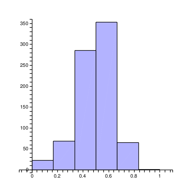
Since a factor of the form $p^{\alpha}$ dominates all of the proven and conjectured bounds on the error given above, we decided to collect data on the values of $\delta={N_{\eqref{fp},g\mathop{\mathsf{}}{ANY},h\mathop{\mathsf{}}{ANY}}(p)-(p-3)}$ for the first 1800 primes (3 through 15413). The data was then tallied based on the value of $\log_{p}{\left|\delta\right|}$. Table 1 and Figure 1 give the data for $\delta\geq 0$, while Table 2 and Figure 2 give the data for $\delta<0$. The case $\delta=0$ did not actually occur in this sample. Likewise, there were no cases where ${\left|delta\right|}>p$, although this is certainly not ruled out for $\delta>0$.

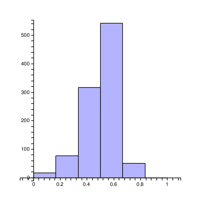
It is not clear whether the greater number of negative values of $\delta$ is significant, or a coincidence of this particular data set. The mean for Table 1 is $0.4943$ and the mean for Table 2 is $0.5050$. This may reflect the same apparent bias towards negative values of $\delta$.

Table 3 and Figure 3 give the values of ${\left|\delta\right|}$ for all computed values of $\delta$. The mean for this table is $0.5003$, which suggests that the expected value of $\log_{p}{\left|\delta\right|}$ may in fact be $1/2$, i.e., that the values of $\delta$ may cluster around $\sqrt{p}$. It is not immediately clear how to derive this from the heuristics. The sample standard deviation can be calculated to be $0.1374$, but the data does not appear to be precisely normally distributed. This is confirmed by a chi-squared test for goodness of fit, which returns the extremely small $p$-value of $7.8039\cdot 10^{-34}$.¹¹ 1 The $p$-value here can be interpreted as the chance that a random sample taken from the predicted distribution would deviate from the distribution as a whole at least as much as the observed data did. Thus this set of data is an extremely bad match for the prediction. We are using statistical language in this note even though the data sets do not come from random variables, and are in fact deterministic. Thus, all of the statistical results in this note should be taken with a very large grain of salt. A sample skewness of $-0.6785$ and a sample kurtosis of $3.6516$ can also be computed. This reflects an asymmetric longer left tail (toward smaller values of $\log_{p}{\left|\delta\right|}$) and a somewhat sharper peak than a normal distribution.

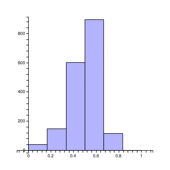
A log-normal distribution was also investigated by taking the exponential function of the midpoints of each of the class intervals. This resulted in a mean of $1.6643$, a sample standard deviation of $0.2196$, a sample skewness of $-0.2366$ and a sample kurtosis of $3.2065$. Thus the shape of the distribution looks more like a normal distribution; however the chi-squared goodness of fit test still gives an extremely small $p$-value of $2.2243\cdot 10^{-10}$. Thus this still does not seem to be the correct distribution. More investigation is clearly necessary, both theoretical and statistical.

The data sets from the tables were collected on a Beowulf cluster, using 16 nodes, each consisting of 2 Pentium III processors running at 1 Ghz. The programming was done in C, using MPI, OpenMP, and OpenSSL libraries. The collection took approximately 60 hours for the 1800 primes between 3 and 15413 (inclusive).

This note is clearly a preliminary effort. The fact that we were unable to interpret the data as any sort of normal distribution is unsatisfying, if not perhaps surprising. We hope in the future to provide at least a conjectural explanation of this data. A better theoretical understanding of the error terms in the theorems we have cited would of course be helpful in this.

The project of extending our analysis to three-cycles and more generally $k$-cycles for small values of $k$, mentioned in previous papers, still remains to be done. Along similar lines, Igor Shparlinski has suggested attempting to analyze the average length of a cycle. Daniel Cloutier, a student at the Rose-Hulman Institute of Technology, has recently begun to collect data which we hope will shed light on both of these problems.

The author would like to thank Pieter Moree for providing the heuristics for estimating the standard deviation $\sigma$ of $F_{g\mathop{\mathsf{}}{ANY},h\mathop{\mathsf{}}{ANY}}(p)$ and for several other results cited in this note. He would also like to thank Diane Evans of the Rose-Hulman Institute of Technology Mathematics Department for statistical advice. Finally, he would like to thank the editor for several helpful suggestions.

References

- [1] Manuel Blum and Silvio Micali. How to generate cryptographically strong sequences of pseudorandom bits. SIAM J. Comput., 13(4):850–864, 1984.
- [2] Mariana Campbell. On fixed points for discrete logarithms. Master’s thesis, University of California at Berkeley, Spring 2003.
- [3] Cristian Cobeli and Alexandru Zaharescu. An exponential congruence with solutions in primitive roots. Rev. Roumaine Math. Pures Appl., 44(1):15–22, 1999.
- [4] Étienne Fouvry. Théorème de Brun-Titchmarsh: Application au théorème de Fermat. Invent. Math., 79(2):383–407, 1985.
- [5] Rosario Gennaro. An improved pseudo-random generator based on discrete log. In Mihir Bellare, editor, Advances in Cryptology — CRYPTO 2000, pages 469Ж481. Springer, 2000.
- [6] Richard K. Guy. Unsolved Problems in Number Theory. Springer-Verlag, 1981.
- [7] Joshua Holden and Pieter Moree. Some heuristics and results for small cycles of the discrete logarithm. Mathematics of Computation. To appear. http://xxx.lanl.gov/abs/math.NT/0401013.
- [8] Joshua Holden and Pieter Moree. New conjectures and results for small cycles of the discrete logarithm. In Alf van der Poorten and Andreas Stein, editors, High Primes and Misdemeanours: lectures in honour of the 60th birthday of Hugh Cowie Williams, number 41 in Fields Institute Communications, pages 245–254. American Mathematical Society, 2004. http://xxx.lanl.gov/abs/math.NT/0305305.
- [9] Sarvar Patel and Ganapathy S. Sundaram. An efficient discrete log pseudo-random generator. In Hugo Krawczyk, editor, Advances in Cryptology — CRYPTO ’98, pages 304–317. Springer, 1998.
- [10] Wen Peng Zhang. On a problem of Brizolis. Pure Appl. Math., 11(suppl.):1–3, 1995.