Enumerative tropical algebraic geometry in $\mathbb{R}^{2}$ Thanks: The author would like to acknowledge a partial support of the NSF and NSERC

Grigory Mikhalkin Address: Department of Mathematics
University of Toronto
100 St. George St.
Toronto, Ontario, M5S 3G3 Canada Address: St. Petersburg Branch of Steklov Mathematical Institute, Fontanka 27, St. Petersburg, 191011 Russia Email address: mikha@math.toronto.edu

Abstract.

The paper establishes a formula for enumeration of curves of arbitrary genus in toric surfaces. It turns out that such curves can be counted by means of certain lattice paths in the Newton polygon. The formula was announced earlier in [18].

The result is established with the help of the so-called tropical algebraic geometry. This geometry allows one to replace complex toric varieties with the real space $\mathbb{R}^{n}$ and holomorphic curves with certain piecewise-linear graphs there.

Key words and phrases:

Tropical curves, enumerative geometry, Gromov-Witten invariants, toric surfaces

2000 Mathematics Subject Classification

Primary: 14N35, 52B20 Secondary: 14N10, 14P25, 51M20

1. Introduction

Recall the basic enumerative problem in the plane. Let $g\geq 0$ and $d\geq 1$ be two numbers and let $\mathcal{Z}=(z_{1},\dots,z_{3d-1+g})$ be a collection of points $z_{j}\in{\mathbb{C}}{\mathbb{P}}^{2}$ in general position. A holomorphic curve $C\subset{\mathbb{C}}{\mathbb{P}}^{2}$ is parameterized by a Riemann surface $\tilde{C}$ under a holomorphic map $\phi:\tilde{C}\to{\mathbb{C}}{\mathbb{P}}^{2}$ so that $C=\phi(\tilde{C})$ . Here we choose the minimal parametrization, i.e. such that no component of $\tilde{C}$ is mapped to a point by $\phi$ . The curve $C$ is irreducible if and only if $\tilde{C}$ is connected. The number $N^{\operatorname{irr}}_{g,d}$ of irreducible curves of degree $d$ and genus $g$ passing through $\mathcal{Z}$ is finite and does not depend on the choice of $z_{j}$ as long as this choice is generic.

Similarly we can set up the problem of counting all (not necessarily irreducible) curves. Define the genus of $C\subset{\mathbb{C}}{\mathbb{P}}^{2}$ to be $\frac{1}{2}(2-\chi(\tilde{C}))$ . Note that the genus can take negative values for reducible curves. The number $N^{\operatorname{mult}}_{g,d}$ of curves of degree $d$ and genus $g$ passing through $\mathcal{Z}$ is again finite and does not depend on the choice of $z_{j}$ as long as this choice is generic. Figure 1 lists some (well-known) first few numbers $N^{\operatorname{irr}}_{g,d}$ and $N^{\operatorname{mult}}_{g,d}$ .

$g\backslash d$ 1 2 3 4 0 1 1 12 620 1 0 0 1 225 2 0 0 0 27 3 0 0 0 1 $g\backslash d$ 1 2 3 4 -1 0 3 21 666 0 1 1 12 675 1 0 0 1 225 2 0 0 0 27

Figure 1. Numbers

N^{\operatorname{irr}}_{g,d}

and

N^{\operatorname{mult}}_{g,d}

The numbers $N^{\operatorname{irr}}_{g,d}$ are known as the Gromov-Witten invariants of ${\mathbb{C}}{\mathbb{P}}^{2}$ (see [12]) while the numbers $N^{\operatorname{mult}}_{g,d}$ are sometimes called the multicomponent Gromov-Witten invariant. One series of numbers determines another by a simple combinatorial relation (see e.g. [3]). A recursive relation which allows one to compute the numbers $N^{\operatorname{irr}}_{0,d}$ (and thus the numbers $N^{\operatorname{mult}}_{0,d}$ ) was given by Kontsevich. This relation came from the associativity of the quantum cohomology (see [12]). In the arbitrary genus case Caporaso and Harris [3] gave an algorithm (bases on a degeneration of ${\mathbb{C}}{\mathbb{P}}^{2}$ ) which allows one to compute the numbers $N^{\operatorname{mult}}_{g,d}$ (and thus the numbers $N^{\operatorname{irr}}_{g,d}$ ).

The main result of this paper gives a new way of computation of these numbers as well as the $\mathbb{R}$ -counterparts of these numbers (that appear in real algebraic geometry). The number $N^{\operatorname{mult}}_{g,d}$ turns out to be the number of certain lattice paths of length $3d-1+g$ in the triangle $\Delta_{d}\subset\mathbb{R}^{2}$ with vertices $(0,0)$ , $(d,0)$ and $(0,d)$ . The paths have to be counted with certain non-negative multiplicities. Furthermore, this formula works not only for ${\mathbb{C}}{\mathbb{P}}^{2}$ but for other toric surfaces as well. For other toric surfaces we just have to replace the triangle $\Delta_{d}$ by other convex lattice polygons. The polygon should be chosen so that it determines the corresponding (polarized) toric surface.

The formula comes as an application of the so-called tropical geometry whose objects are certain piecewise-linear polyhedral complexes in $\mathbb{R}^{n}$ . These objects are the limits of the amoebas of holomorphic varieties after a certain degeneration of the complex structure. The idea to use these objects for enumeration of holomorphic curves is due to Kontsevich.

In [13] Kontsevich and Soibelman proposed a program linking Homological Mirror Symmetry and torus fibrations from the Strominger-Yau-Zaslow conjecture [26]. The relation is provided by passing to the so-called “large complex limit” which deforms a complex structure on a manifold to its worst possible degeneration. Similar deformations appeared in other areas of mathematics under different names. The patchworking in Real Algebraic Geometry was discovered by Viro [28]. Maslov and his school studied the so-called dequantization of the semiring of positive real numbers (cf. [15]). The limiting semiring is isomorphic to the $(\max,+)$ -semiring ${\mathbb{R}}_{\operatorname{trop}}$ , the semiring of real numbers equipped with taking the maximum for addition and addition for multiplication.

The semiring ${\mathbb{R}}_{\operatorname{trop}}$ is known to computer scientists as one of tropical semirings, see e.g. [20]. In Mathematics this semiring appears from non-Archimedean fields $K$ under a certain pushing forward to $\mathbb{R}$ of the arithmetic operations in $K$ .

In this paper we develop some basic algebraic geometry over ${\mathbb{R}}_{\operatorname{trop}}$ with a view towards counting curves. In particular, we rigorously set up some enumerative problems over ${\mathbb{R}}_{\operatorname{trop}}$ and prove their equivalence to the relevant problems of complex and real algebraic geometry. The reader can refer to Chapter 9 of Sturmfels’ recent book [27] for some first steps in tropical algebraic geometry. See also [24], [23], [25] for some of more recent development.

We solve the corresponding tropical enumerative problem in $\mathbb{R}^{2}$ . As an application we get a formula counting the number of curves of given degree and genus in terms of certain lattice paths of a given length in the relevant Newton polygon. In particular this gives an interpretation of the Gromov-Witten invariants in ${\mathbb{P}}^{2}$ and ${\mathbb{P}}^{1}\times{\mathbb{P}}^{1}$ via lattice paths in a triangle and a rectangle respectively. This formula was announced in [18]. For the proof we use the patchworking side of the story which is possible to use since the ambient space is 2-dimensional and the curves there are hypersurfaces. An alternative approach (applicable to higher dimensions as well) is to use the symplectic field theory of Eliashberg, Givental and Hofer [4]. Generalization of this formula to higher dimensions is a work in progress. In this paper we only define the enumerative multiplicity for the 2-dimensional case. There is a similar definition (though no longer localized at the vertices) for multiplicities of isolated curves in higher-dimensional tropical enumerative problems. However, in higher dimensions there might be families of tropical curves (of positive genus) for enumerative problems with finite expected numbers of solutions (this phenomenon already appears for curves in $\mathbb{R}^{3}$ passing through a finite collection of points in general position) which seem to pose a serious problem (that perhaps asks for development of tropical virtual classes).

The main theorems are stated in section 7 and proved in section 8. In section 2 we define tropical curves geometrically (in a way similar to webs of Aharony, Hanany and Kol [1], [2]). In section 3 we exhibit them as algebraic objects over the tropical semifield. In section 4 we define the tropical enumerative problems in $\mathbb{R}^{2}$ , in section 5 recall those in $(\mathbb{C}^{*})^{2}$ . Section 6 is auxiliary for section 8 and deals with certain piecewise-holomorphic piecewise-Lagrangian objects in $(\mathbb{C}^{*})^{2}$ called complex tropical curves. An outline of the approach taken in this paper can also be found in [8]. A somewhat different approach can be found in [21].

The author is grateful to Y. Eliashberg, K. Hori, I. Itenberg, M. Kapranov, M. Kontsevich, A. Okounkov, B. Sturmfels, R. Vakil, O. Viro and J.-Y. Welschinger for useful discussions. The author is also indebted to the referees for thorough and helpful remarks, corrections and suggestions as well as to B. Bertrand, F. Bihan and H. Markwig who found many inconsistencies and misprints in earlier versions of the paper.

2. Tropical curves as graphs in $\mathbb{R}^{n}$

In this section we geometrically define tropical curves in $\mathbb{R}^{n}$ and set up the corresponding enumerative problem. We postpone the algebraic treatment of the tropical curves (which explains the term “tropical” among other things) until the next section.

2.1. Definitions and the first examples

Let $\bar{\Gamma}$ be a weighted finite graph. The weights are natural numbers prescribed to the edges. Clearly, $\bar{\Gamma}$ is a compact topological space. We make it non compact by removing the set of all 1-valent vertices $\mathcal{V}_{1}$ ,

\Gamma=\bar{\Gamma}\smallsetminus{\mathcal{V}_{1}}.

Remark 2.1.

Removal of the 1-valent vertices is due to a choice we made in the algebraic side of the treatment. In this paper we chose the semifield ${\mathbb{R}}_{\operatorname{trop}}=(\mathbb{R},\max,+)$ as our “ground semifield” for tropical variety, see the next section. The operation $\max$ plays the rôle of addition and thus we do not have an additive zero. Non-compactness of $\Gamma$ is caused by this choice. Should we have chosen ${\mathbb{R}}_{\operatorname{trop}}\cup\{-\infty\}$ instead for our ground semifield we wouldn’t need to remove the 1-valent vertices but then we would have to consider tropical toric compactification of the ambient space $\mathbb{R}^{n}$ as well. The approach of this paper is chosen for the sake of simplicity. The other approach has its own advantages and will be realized in a forthcoming paper.

Definition 2.2.

A proper map $h:\Gamma\to\mathbb{R}^{n}$ is called a parameterized tropical curve if it satisfies to the following two conditions.

•

For every edge $E\subset\Gamma$ the restriction $h|_{E}$ is either an embedding or a constant map. The image $h(E)$ is contained in a line $l\subset\mathbb{R}^{2}$ such that the slope of $l$ is rational.
•

For every vertex $V\in\Gamma$ we have the following property. Let $E_{1},\dots,E_{m}\subset\Gamma$ be the edges adjacent to $V$ , let $w_{1},\dots,w_{m}\in\mathbb{N}$ be their weights and let $v_{1},\dots,v_{m}\in\mathbb{Z}^{n}$ be the primitive integer vectors at the point $h(V)$ in the direction of the edges $h(E_{j})$ (we take $v_{j}=0$ if $h(E_{j})$ is a point). We have

(1) $\sum\limits_{j=1}^{m}w_{j}v_{j}=0.$

We say that two parameterized tropical curves $h:\Gamma\to\mathbb{R}^{n}$ and $h^{\prime}:\Gamma^{\prime}\to\mathbb{R}^{n}$ are equivalent if there exists a homeomorphism $\Phi:\Gamma\to\Gamma^{\prime}$ which respects the weights of the edges and such that $h=h^{\prime}\circ\Phi$ . We do not distinguish equivalent parameterized tropical curves. The image

C=h(\Gamma)\subset\mathbb{R}^{n}

is called the unparameterized tropical curve or just a tropical 1-cycle if no connected component of $\Gamma$ gets contracted to a point. The 1-cycle $C$ is a piecewise-linear graph in $\mathbb{R}^{n}$ with natural weights on its edges induced from the weights on $\Gamma$ . If $E$ is an edge of $C$ then $h^{-1}(E)$ is a union of subintervals of the edges of $\Gamma$ . The weight of $E$ is the sum of the weights of these edges.

Remark 2.3.

In dimension 2 the notion of tropical curve coincides with the notion of $(p,q)$ -webs introduced by Aharony, Hanany and Kol in [2] (see also [1]).

Remark 2.4.

The map $h$ can be used to induce a certain structure on $\Gamma$ from the affine space $\mathbb{R}^{n}$ . It is an instance of the so-called $\mathbb{Z}$ -affine structure. For a graph $\Gamma$ such a structure is equivalent to a metric for every edge of $\Gamma$ . Here is a way to obtain such a metric for the edges that are not contracted to a point.

Let $E\subset\Gamma$ be a compact edge of weight $w$ that is not contracted to a point by $h$ . Such edge is mapped to a finite straight interval with a rational slope in $\mathbb{R}^{n}$ . Let $l$ be the length of a primitive rational vector in the direction of $h(E)$ . We set the length of $E$ to be $\frac{|h(E)|}{lw}$ .

Note that $\Gamma$ also has non-compact edges (they result from removing one-valent vertices from $\bar{\Gamma}$ ). Such edges are mapped to unbounded straight intervals by $h$ .

It is possible to consider abstract tropical curves as graphs equipped with such $\mathbb{Z}$ -affine structures. Then tropical maps (e.g. to $\mathbb{R}^{n}$ ) will be maps that respect such structure. Abstract tropical curves have genus (equal to $b_{1}(\Gamma)$ ) and the number of punctures (equal to the number of ends of $\Gamma$ ) and form moduli space in a manner similar to that of the classical Riemann surfaces. This point of view will be developed in a forthcoming paper.

Example 2.5.

Consider the union of three simple rays

Y=\{(x,0)\ |\ x\leq 0\}\cup\{(0,y)\ |\ y\leq 0\}\cup\{(x,x)\ |\ x\geq 0\}\subset\mathbb{R}^{2}.

This graph (considered as a tautological embedding in $\mathbb{R}^{2}$ ) is a tropical curve since $(-1,0)+(0,-1)+(1,1)=0$ . A parallel translation of $Y$ in any direction in $\mathbb{R}^{2}$ is clearly also a tropical curve. This gives us a 2-dimensional family of curves in $\mathbb{R}^{2}$ . Such curves are called tropical lines.

Remark 2.6.

The term tropical line is justified in the next section dealing with the underlying algebra. So far we would like to note the following properties of this family, see Figure 2.

•

For any two points in $\mathbb{R}^{2}$ there is a tropical line passing through them.
•

Such a line is unique if the choice of these two points is generic.
•

Two generic tropical lines intersect in a single point.

Refer to caption — Figure 2. Three distinct tropical lines.

Somewhat more complicated tropical curves (corresponding to projective curves of degree 3) are pictured on Figure 3

2.2. The degree of a tropical curve in $\mathbb{R}^{n}$

Let ${\mathcal{T}}=\{\tau_{1},\dots,\tau_{q}\}\subset\mathbb{Z}^{n}$ be a set of non-zero integer vectors such that $\sum\limits_{j=1}^{q}\tau_{j}=0$ . Suppose that in this set we do not have positive multiples of each other, i.e. if $\tau_{j}=m\tau_{k}$ for $m\in\mathbb{N}$ then $\tau_{j}=\tau_{k}$ . The degree of a tropical 1-cycle $C\subset\mathbb{R}^{n}$ takes values in such sets according to the following construction.

By our definition a tropical curve $h:\Gamma\to\mathbb{R}^{n}$ has a finite number of ends, i.e. unbounded edges (rays). Let $\tau\in\mathbb{Z}^{n}$ be a primitive vector. A positive multiple of $\tau$ is included in ${\mathcal{T}}$ if and only if there exists an end of $\Gamma$ which is mapped in the direction of $\tau$ . In such case we include $m\tau$ into ${\mathcal{T}}$ , where $m$ is the sum of multiplicities of all such rays.

Definition 2.7.

The resulting set ${\mathcal{T}}$ is called the toric degree of $C\subset\mathbb{R}^{n}$ . Accordingly, the degree of a parameterized tropical curve $h:\Gamma\to\mathbb{R}^{n}$ is the degree of its image $h(\Gamma)$ .

Note that the sum of all vectors in ${\mathcal{T}}$ is zero. This follows from adding the conditions (1) from Definition 2.2 in all vertices of $C$ .

For example the degree of both curves from Figure 5 is $\{(-1,-1)$ , $(2,-1)$ , $(-1,2)\}$ while the degree of both curves from Figure 3 is $\{(-3,0),(0,-3),(3,3)\}$ .

Definition 2.8.

If the toric degree of a tropical 1-cycle $C\subset\mathbb{R}^{n}$ is $\{(-d,0,\dots,0),\dots,(0,\dots,0,-d),(d,\dots,d)\}$ then $C$ is called a tropical projective curve of degree $d$ .

The curves from Figure 3 are examples of planar projective cubics.

2.3. Genus of tropical curves and tropical 1-cycles

We say that a tropical curve $h:\Gamma\to\mathbb{R}^{n}$ is reducible if $\Gamma$ is disconnected. We say that a tropical 1-cycle $C\subset\mathbb{R}^{n}$ is reducible if it can be presented as a union of two distinct tropical 1-cycles. Clearly, every reducible 1-cycle can be presented as an image of a reducible parameterized curve.

Definition 2.9.

The genus of a parameterized tropical curve $\Gamma\to\mathbb{R}^{n}$ is $\dim H_{1}(\Gamma)-\dim H_{0}(\Gamma)+1$ . In particular, for irreducible parameterized curves the genus is the first Betti number of $\Gamma$ . The genus of a tropical 1-cycle $C\subset\mathbb{R}^{n}$ is the minimum genus among all parameterizations of $C$ .

Note that according to this definition the genus can be negative. E.g. the union of the three lines from Figure 2 has genus $-2$ .

If $C\subset\mathbb{R}^{n}$ is an embedded 3-valent graph then the parameterization is unique. However, in general, there might be several parameterizations of different genus and taking the minimal value is essential.

Example 2.10.

The tropical 1-cycle on the right-hand side of Figure 3 can be parameterized by a tree once we “resolve” its 4-valent vertex to make the parameterization domain into a tree. Therefore, its genus is 0.

2.4. Deformations of tropical curves within their combinatorial type

As in the classical complex geometry case the deformation space of a tropical curve $h:\Gamma\to\mathbb{R}^{n}$ is subject to the constraint coming from the Riemann-Roch formula. Let $x$ be the number of ends of $\Gamma$ .

Remark 2.11.

The number $-x$ is a tropical counterpart of the value of the canonical class of the ambient complex variety on the curve $h(\Gamma)$ . The ambient space $\mathbb{R}^{n}$ corresponds to the torus $(\mathbb{C}^{*})^{n}$ classically. Let $V\subset(\mathbb{C}^{*})^{n}$ be a holomorphic curve with a finite number of ends. The space $(\mathbb{C}^{*})^{n}$ is not compact, but one can always choose a toric compactification $\mathbb{C}T\supset(\mathbb{C}^{*})^{n}$ such that every point of the closure $\bar{V}\supset V$ in $\mathbb{C}T$ intersects not more than one boundary divisor (i.e. a component of $\mathbb{C}T\smallsetminus(\mathbb{C}^{*})^{n}$ ). Then every end of $V$ can be prescribed a multiplicity equal to the intersection number of the point of $\bar{V}$ and the corresponding boundary divisor. The value of the canonical class of $\mathbb{C}T$ on $\bar{V}$ equals to the sum of these multiplicities.

Definition 2.12.

The curves $h:\Gamma\to\mathbb{R}^{n}$ and $h^{\prime}:\Gamma\to\mathbb{R}^{n}$ (parameterized by the same graph $\Gamma$ ) are said to be of the same combinatorial type if for any edge $E\subset\Gamma$ the segments $h(E)$ and $h^{\prime}(E)$ are parallel.

Note that if two tropical curves $\Gamma\to\mathbb{R}^{n}$ are isotopic in the class of tropical curves (with the same domain $\Gamma$ ) then they are of the same combinatorial type.

The valence of a vertex of $\Gamma$ is the number of adjacent edges regardless of their weights. The graph $\Gamma$ is called 3-valent if every its vertex is 3-valent. The parameterized tropical curve $h:\Gamma\to\mathbb{R}^{n}$ is called 3-valent if $\Gamma$ is 3-valent.

Proposition 2.13.

Let $\Gamma$ be a 3-valent graph. The space of all tropical curves $\Gamma\to\mathbb{R}^{n}$ in the same combinatorial type (up to their equivalence from Definition 2.2) is an open convex polyhedral domain in a real affine $k$ -dimensional space, where

k\geq x+(n-3)(1-g).

Proof.

It suffices to prove this for a connected graph $\Gamma$ since different components of $\Gamma$ vary independently. and, furthermore, both sides of the inequality are additive with respect to taking the union of components (note that $1-g=b_{0}(\Gamma)-b_{1}(\Gamma)=\chi(\Gamma)$ ). Let $\Gamma^{\prime}\subset\Gamma$ be a finite tree containing all the vertices of $\Gamma$ . Note that the number of finite edges in $\Gamma\smallsetminus\Gamma^{\prime}$ is $g$ . By an Euler characteristic computation we get that the number of finite edges of $\Gamma^{\prime}$ is equal to $x-3+2g$ .

Maps $\Gamma^{\prime}\to\mathbb{R}^{n}$ vary in a linear $(x-3+2g+n)$ -dimensional family if we do not change the slopes of the edges. The $(x-3+2g)$ -dimensional part comes from varying of the lengths of the edges while the $n$ -dimensional part comes from translations in $\mathbb{R}^{n}$ . Such a map is extendable to a tropical map $\Gamma\to\mathbb{R}^{n}$ if the pairs of vertices corresponding to the $g$ remaining edges define the lines with the correct slope. Each of the $g$ edges imposes a linear condition of codimension at most $n-1$ . Thus tropical perturbations of $\Gamma\to\mathbb{R}^{n}$ are contained in a linear family of dimension at least $x-3+2g+n-(n-1)g=x+(n-3)(1-g)$ . They form an open convex polyhedral domain there defined by the conditions that the lengths of all the edges are positive. ∎

Consider the general case now and suppose that $\Gamma$ has vertices of valence higher than 3. How much $\Gamma$ differs from a 3-valent graph is measured by the following characteristic. Let the overvalence $\operatorname{ov}(\Gamma)$ be the sum of the valences of all vertices of valence higher than 3 minus the number of such vertices. Thus $\operatorname{ov}(\Gamma)=0$ if and only if no vertex of $\Gamma$ has valence higher than 3.

Proposition 2.14.

The space of all tropical curves $\Gamma\to\mathbb{R}^{n}$ in the same combinatorial type (up to their equivalence from Definition 2.2) is an open convex polyhedral domain in a real affine $k$ -dimensional space, where

k\geq x+(n-3)(1-g)-\operatorname{ov}(\Gamma)-c,

where $c$ is the number of edges of $\Gamma$ that are mapped to a point.

Proof.

The proof is similar to that of Proposition 2.13. If the image of an edge is a point in $\mathbb{R}^{n}$ then we cannot vary its length. Similarly we are lacking some degrees of freedom (with respect to the set-up of Proposition 2.13) if $\operatorname{ov}>0$ . ∎

Note that $\operatorname{ov}+c$ can be interpreted as the overvalence of the image $h(\Gamma)$ .

2.5. Changing the combinatorial type of $\Gamma$

Sometimes we can deform $\Gamma$ and $h:\Gamma\to\mathbb{R}^{n}$ by the following procedure reducing $\operatorname{ov}$ . If we have $n>3$ edges adjacent to the same vertex then we can separate them into two groups so that each group contains at least 2 edges. Let us insert a new edge $E^{\prime}$ separating these groups as shown in Figure 4. This replaces the initial $n$ -valent vertex with 2 vertices (the endpoints of $E^{\prime}$ ) of smaller valence. There is a “virtual slope” of $E^{\prime}$ determined by the slopes of the edges in each group. This is the slope to appear in local perturbation of the tropical map $h:\Gamma\to\mathbb{R}^{n}$ (if such a perturbation exists). Note that the weight of the new edge does not have to be equal to 1.

There is another modification of a tropical curve near its vertex by changing the combinatorial type of $\Gamma$ which works even for some 3-valent vertices.

Example 2.15.

Let $\Gamma$ be the union of 3 rays in $\mathbb{R}^{2}$ in the direction $(-2,1)$ , $(1,-2)$ and $(1,1)$ emanating from the origin (pictured on the left-hand side of Figure 5). This curve is a simple tropical curve of genus 0.

It can be obtained as a $t\to 0$ limit of the family of genus 1 curves given by the union of 3 rays in $\mathbb{R}^{2}$ in the direction $(-2,1)$ , $(1,-2)$ and $(1,1)$ emanating from and $(-2t,t)$ , $(t,-2t)$ and $(t,t)$ respectively and the three intervals $[(-2t,t),(t,-2t)]$ , $[(-2t,t),(t,t)]$ and $[(t,t),(t,-2t)]$ as pictured in Figure 5.

Let $V$ be a 3-valent vertex of $\Gamma$ . As in Definition 2.2 let $w_{1},w_{2},w_{3}$ be the weights of the edges adjacent to $V$ and let $v_{1},v_{2},v_{3}$ be the primitive integer vectors in the direction of the edges.

Definition 2.16.

The multiplicity of $C$ at its 3-valent vertex $V$ is $w_{1}w_{2}|v_{1}\wedge v_{2}|$ . Here $|v_{1}\wedge v_{2}|$ is the area of the parallelogram spanned by $v_{1}$ and $v_{2}$ . Note that

w_{1}w_{2}|v_{1}\wedge v_{2}|=w_{2}w_{3}|v_{2}\wedge v_{3}|=w_{3}w_{1}|v_{3}\wedge v_{1}|

since $v_{1}w_{1}+v_{2}w_{2}+v_{3}w_{3}=0$ by Definition 2.2.

Note that the multiplicity of a vertex is always divisible by the product of the weights of any two out of the three adjacent edges.

Definition 2.17.

We say that $h^{\prime}:\Gamma^{\prime}\to\mathbb{R}^{n}$ is a perturbation of $h:\Gamma\to\mathbb{R}^{n}$ if there exists a family $h^{\prime}_{t}:\Gamma^{\prime}\to\mathbb{R}^{n}$ , $t>0$ , in the same combinatorial type as $h^{\prime}$ and the pointwise limit $h^{\prime}_{0}=\lim\limits_{t\to 0}h^{\prime}_{t}$ such that $h^{\prime}_{0}(\Gamma^{\prime})$ coincides with $h(\Gamma)$ (as tropical 1-cycles).

Definition 2.18.

A tropical curve $h:\Gamma\to\mathbb{R}^{n}$ is called smooth if $\Gamma$ is 3-valent, $h$ is an embedding and the multiplicity of every vertex of $C$ is 1.

Proposition 2.19.

A smooth curve does not admit perturbations of different combinatorial types.

Proof.

Suppose that $h^{\prime}_{t}:\Gamma^{\prime}\to\mathbb{R}^{n}$ is a perturbation of a smooth curve $h:\Gamma\to\mathbb{R}^{n}$ . Since $h$ is an embedding and $h(\Gamma)=h^{\prime}_{0}(\Gamma^{\prime})$ we have a map

\psi:\Gamma^{\prime}\to\Gamma.

Note that the weight of every edge from $\Gamma$ is 1 since otherwise the endpoints of multiple edges would have multiplicity greater than 1. Thus the inverse image of every open edge of $\Gamma$ under $\psi$ is a single edge of $\Gamma^{\prime}$ .

Thus $\psi$ must be a homeomorphism near the inner points of the edges of $\Gamma^{\prime}$ . Let $a\in\Gamma$ be a vertex and $U\ni a$ be its small neighborhood in $\Gamma$ . Note that $\psi^{-1}(U)$ is connected since $a$ is 3-valent (otherwise we can divide the adjacent edges to $a$ into two groups with zero sums of the primitive integer vectors).

Suppose that $\psi^{-1}(a)$ is not a point. Then $\psi^{-1}(a)$ is a graph which has 3 distinguished vertices that are adjacent to the edges of $\psi^{-1}(U)\smallsetminus\psi^{-1}(a)$ . The graph $A=\psi^{\prime}_{t}(\psi^{-1}(U))$ must be contained in the affine 2-plane in $\mathbb{R}^{n}$ containing the ends $A$ . This follows from the balancing condition for $A$ .

The 3-valent vertices of $A$ have multiplicities from Definition 2.16. Since $A$ is planar we can extend the definition of the multiplicity to higher-valent vertices as follows. Let $V\in A$ be a $k$ -valent vertex, $v_{1},\dots,v_{k}$ be the primitive integer vectors in the directions of the adjacent edges to $A$ numbered consistently with the cyclic order in the ambient 2-plane and $w_{1},\dots,w_{k}$ be the corresponding weights. We set the multiplicity of $V$ to be

\prod\limits_{l=2}^{k-1}|v_{l}\wedge\sum\limits_{j=1}^{l}v_{j}|.

It is easy to see that the multiplicity of $a$ in $\Gamma$ is equal to the sum of multiplicities of all the vertices of $A$ . The multiplicities of all vertices are positive integers. Therefore, the multiplicity of $a$ is greater than $1$ unless $\psi^{-1}(a)$ is a point. ∎

Proposition 2.13 can be generalized in the following way to incorporate possible perturbations.

Proposition 2.20.

The space of deformations of a parameterized tropical curve $h:\Gamma\to\mathbb{R}^{n}$ is locally a cone

{\mathcal{C}}=\bigcup\limits_{j}{\mathcal{C}_{j}},

where ${\mathcal{C}_{j}}$ is a polyhedral convex cone corresponding to tropical curves parameterized by perturbations $\Gamma_{j}\to\mathbb{R}^{n}$ of $h:\Gamma\to\mathbb{R}^{n}$ of a given combinatorial type. The union is taken over all possible combinatorial types of perturbations. We have

\dim{\mathcal{C}_{j}}\geq x+(n-3)(1-g)-\operatorname{ov}(\Gamma_{j})-c,

where $c$ is the number of the edges of $\Gamma_{j}$ that are mapped to a point.

Proof.

This proposition follows from Proposition 2.14 applied to all possible perturbation of $\Gamma$ . ∎

Remark 2.21.

Not all conceivable perturbations of $h:\Gamma\to\mathbb{R}^{n}$ are realized as the following example shows. Let $C_{1}\subset\mathbb{R}^{2}\times\{0\}\subset\mathbb{R}^{3}$ be a tropical 1-cycle of genus 1. Let $C_{2}=\{y\}\times\mathbb{R}\subset\mathbb{R}^{3}$ be a vertical line such that $y$ is a point on $C_{1}$ such that $C_{1}\smallsetminus\{y\}$ is contractible. The curve

C=C_{1}\cup C_{2}

has a 4-valent vertex that cannot be perturbed (as any such perturbation would force $C_{1}$ out of the plane $\mathbb{R}^{2}\times\{0\}$ ). Thus any 3-valent perturbation of the tautological embedding $C_{1}\cup C_{2}\subset\mathbb{R}^{3}$ has to have an edge mapping to a point.

This phenomenon is related to the so-called superabundancy phenomenon.

2.6. Superabundancy and regularity

Some curves vary in a family strictly larger than “the prescribed dimension” $x+(n-3)(1-g)-\operatorname{ov}-c$ .

Definition 2.22.

A parameterized tropical curve $h:\Gamma\to\mathbb{R}^{n}$ is called regular if the space of the curves of this combinatorial type (which is a polyhedral domain in an affine space by Proposition 2.14) has dimensions $x+(n-3)(1-g)-\operatorname{ov}-c$ . Otherwise it is called superabundant.

In contrast to the classical case tropical superabundancy can be easily seen geometrically. By the proof of Proposition 2.13 the superabundancy appears if the cycles of the graph $\Gamma$ do not provide transversal conditions for the length of the bounded edges of the subtree $\Gamma^{\prime}$ . This is the case if some of the cycles of $C\subset\mathbb{R}^{n}$ are contained in smaller-dimensional affine-linear subspaces of $\mathbb{R}^{n}$ , e.g. if a non-trivial cycle of $\Gamma$ gets contracted or it a spatial curve develops a planar cycle. More generally, this is the case if several non-degenerate “spatial” cycles combine to a degenerate “flat” cycle.

Clearly, no irreducible tropical curve of genus 0 can be superabundant as it has no cycles. Furthermore, tropical immersions of 3-valent graphs to the plane $\mathbb{R}^{2}$ are never superabundant as the following proposition shows.

Proposition 2.23.

Every tropical immersion $h:\Gamma\to\mathbb{R}^{2}$ is regular if $\Gamma$ is 3-valent. If $\Gamma$ has vertices of valence higher than 3 them $h:\Gamma\to\mathbb{R}^{2}$ varies in at most $(x+g-2)$ -dimensional family.

Proof.

Recall the proof of Propositions 2.13 and 2.14. Once again we may assume that $\Gamma$ is connected. Let $V\in\Gamma$ be any vertex.

We may choose an order on the vertices of $\Gamma$ so that it is consistent with the distance from $V$ , i.e. so that the order of a vertex $V^{\prime}$ is greater than the order of a vertex $V^{\prime\prime}$ whenever $V^{\prime}$ is strictly further from $V$ than $V^{\prime\prime}$ . The balancing condition for $h(\Gamma)$ implies the following maximum principle for $\Gamma$ : any vertex of $\Gamma$ is either adjacent to an unbounded edge of $\Gamma$ or is connected with a bounded edge to a higher order vertex. Inductively one may choose a maximal tree $\Gamma^{\prime}\subset\Gamma$ so that this maximum principle also holds for $\Gamma^{\prime}$ . Note that the the set of vertices of $\Gamma^{\prime}$ coincides with the set of vertices of $\Gamma$ . Note also that our choice of order on this set gives the orientation on the edges of $\Gamma$ : every edge is directed from a smaller to a larger vertex.

The space of deformation of $h$ within the same combinatorial type is open in a $k$ -dimensional real affine space that is cut by $g$ hyperplanes in $\mathbb{R}^{l+n}$ where $l$ is the number of bounded edges of $\Gamma^{\prime}$ . Each of these $g$ hyperplanes is non-trivial if $h$ is an immersion and $\Gamma$ is 3-valent, since then there can be no parallel edges adjacent to the same vertex.

We have regularity if these hyperplanes intersect transversely. The hyperplanes are given by a $g\times(l+2)$ -matrix with real values. The rows of this matrix correspond to the edges of $\Gamma\smallsetminus\Gamma^{\prime}$ while the first $l$ columns correspond to the edges of $\Gamma^{\prime}$ (the remaining $2$ columns correspond to translations in $\mathbb{R}^{2}$ ). To show that the rank of this matrix is $g$ in the 3-valent case we exhibit an upper-triangular $g\times g$ -minor with non-zero elements on its diagonal.

For each edge $E$ of $\Gamma\smallsetminus\Gamma^{\prime}$ we include the column corresponding to the (bounded) edge of $\Gamma^{\prime}$ directed toward the highest endpoint of $E$ . If $\Gamma$ is 3-valent different edges of $\Gamma-\Gamma^{\prime}$ correspond under this construction to different edges of $\Gamma^{\prime}$ . This produces the required $g\times g$ -minor.

If $\Gamma$ is not 3-valent then the number of the bounded edges of $\Gamma^{\prime}$ is $x-3+2g-\operatorname{ov}$ . This number is the same as the number of vertices of $\Gamma^{\prime}$ other than $V$ . We can do the construction of the minor as above but only using one edge of $\Gamma\smallsetminus\Gamma^{\prime}$ at every vertex of $\Gamma$ other than $V$ . In such a way we can get a non-degenerate $(g-\operatorname{ov})\times(g-\operatorname{ov})$ -minor and thus the dimension is at most $x-3+2g-\operatorname{ov}-(g-\operatorname{ov})+2=x-1+g$ (2 comes from translations in $\mathbb{R}^{2}$ ). If there exists a vertex of valence higher than 3 then we may choose such a vertex for the root $V$ of the tree $\Gamma^{\prime}$ and this gives a non-degenerate minor of size strictly larger than $(g-\operatorname{ov})$ . ∎

Corollary 2.24.

An immersed 3-valent tropical curve $h:\Gamma\to\mathbb{R}^{n}$ locally varies in a (real) linear $k$ -dimensional space, where

k=x+(n-3)(1-g)

if either $n=2$ or $g=0$ .

Remark 2.25.

There exist superabundant tropical immersions $\Gamma\to\mathbb{R}^{2}$ if $\Gamma$ is not 3-valent. A nice example is given by the Pappus theorem configuration that is a union of 9 lines, see Figure 6.

Assume that the nine Pappus lines have rational slopes and take $\Gamma$ to be their union in $\mathbb{R}^{2}$ so that our tropical curve $\Gamma\to\mathbb{R}^{2}$ is a tautological embedding. We have $x=18$ , $g=22$ , $\operatorname{ov}=39$ , $c=0$ . Therefore $x+g-1-\operatorname{ov}-c=0$ , yet our configuration varies at least in a 3-dimensional family (as we can apply any translation and homothety in $\mathbb{R}^{2}$ without changing the slopes of our lines.

Clearly, there also exist superabundant immersed 3-valent tropical curves in $\mathbb{R}^{n}$ , $n>2$ . E.g. if $h:\Gamma\to\mathbb{R}^{2}$ is a (regular) tropical immersion of a 3-valent graph $\Gamma$ then its composition with the embedding $\mathbb{R}^{2}\subset\mathbb{R}^{n}$ , $n>2$ , is superabundant.

3. Underlying tropical algebra

In this section we exhibit the tropical curves as algebraic varieties with respect to a certain algebra and also define some higher-dimensional tropical algebraic varieties in $\mathbb{R}^{n}$ .

3.1. The tropical semifield ${\mathbb{R}}_{\operatorname{trop}}$

Consider the semiring ${\mathbb{R}}_{\operatorname{trop}}$ of real numbers equipped with the following arithmetic operations called tropical in Computer Science:

``x+y"=\max\{x,y\}\hskip 20.0pt``xy"=x+y,

$x,y\in{\mathbb{R}}_{\operatorname{trop}}$ . We use the quotation marks to distinguish the tropical operations from the classical ones. Note that addition is idempotent, $``x+x=x"$ . This makes ${\mathbb{R}}_{\operatorname{trop}}$ to a semiring without the additive zero (the role of such zero would be played by $-\infty$ ).

Remark 3.1.

According to [20] the term “tropical” appeared in Computer Science in honor of Brazil and, more specifically, after Imre Simon (who is a Brazilian computer scientist) by Dominique Perrin. In Computer Science the term is usually applied to $(\min,+)$ semirings. Our semiring ${\mathbb{R}}_{\operatorname{trop}}$ is $(\max,+)$ by our definition but isomorphic to the $(\min,+)$ -semiring, the isomorphism is given by $x\mapsto-x$ .

As usual, a (Laurent) polynomial in $n$ variables over ${\mathbb{R}}_{\operatorname{trop}}$ is defined by

f(x)=``\sum\limits_{j\in A}a_{j}x^{j}"=\max\limits_{j\in A}(<j,x>+a_{j}),

where $x=(x_{1},\dots,x_{n})\in\mathbb{R}^{n}$ , $j=(j_{1},\dots,j_{n})$ , $x^{j}=x_{1}^{j_{1}}\dots x_{n}^{j_{n}}$ , ${<j,x>}=j_{1}x_{1}+\dots+j_{n}x_{n}$ and $A\subset\mathbb{Z}^{n}$ is a finite set. Note that $f:\mathbb{R}^{n}\to\mathbb{R}$ is a convex piecewise-linear function. It coincides with the Legendre transform of a function $j\mapsto-a_{j}$ defined on the finite set $A$ .

Definition 3.2.

The polyhedron $\Delta=\operatorname{ConvexHull}(A)$ is called the Newton polyhedron of $f$ . It can be treated as a refined version of the degree of the polynomial $f$ in toric geometry.

3.2. Tropical hypersurfaces: the variety of a tropical polynomial

For a tropical polynomial $f$ in $n$ variables we define its variety $V_{f}\subset\mathbb{R}^{n}$ as the set of points where the piecewise-linear function $f$ is not smooth, cf. [10], [18] and [27]. In other words, $V_{f}$ is the corner locus of $f$ .

Proposition 3.3.

$V_{f}$ is the set of points in $\mathbb{R}^{n}$ where more than one monomial of $f$ reaches its maximal value.

Proof.

If exactly one monomial of $f(x)=``\sum\limits_{j\in A}a_{j}x^{j}"=\max\limits_{j\in A}(<j,x>+a_{j})$ is maximal at $x\in\mathbb{R}^{n}$ then $f$ locally coincides with this monomial and, therefore, linear and smooth. Otherwise $f$ has a corner at $x$ . ∎

Remark 3.4.

At a first glance this definition might appear to be unrelated to the classical definition of the variety as the zero locus of a polynomial. To see a connection recall that there is no additive zero in ${\mathbb{R}}_{\operatorname{trop}}$ , but its rôle is played by $-\infty$ .

Consider the graph $\Gamma_{f}\subset\mathbb{R}^{n}\times\mathbb{R}$ of a tropical polynomial $f:\mathbb{R}^{n}\to\mathbb{R}$ . The graph $\Gamma_{f}$ itself is not a tropical variety in $\mathbb{R}^{n+1}$ but it can be completed to the tropical variety

\bar{\Gamma}_{f}=\Gamma_{f}\cup\{(x,y)\ |\ x\in V_{f},\ y\leq f(x)\},

see Figure 7.

Proposition 3.5.

$\bar{\Gamma}_{f}$ coincides with the variety of the polynomial in $(n+1)$ variables $``y+f(x)"$ (where $y\in\mathbb{R}$ , $x\in\mathbb{R}^{n}$ ).

Proof.

If $(x,y)\in\Gamma_{f}$ then we have $y$ and one of the monomials of $f$ both reaching the maximal values in $``y+f(x)"=\max\{y,f(x)\}$ . If $x\in V_{f}$ and $y<f(x)$ then two monomials of $f(x)$ are reaching the maximal value at the expression $``y+f(x)"$ . ∎

Note that we have $V_{f}=\bar{\Gamma}_{f}\cap\{y=t\}$ for $t$ sufficiently close to $-\infty$ . This is the sense in which $V_{f}$ can be thought as a zero locus.

One may argue that $\Gamma_{f}$ itself is a subtropical variety (as in subanalytic vs. analytic sets) while $\bar{\Gamma}_{f}$ is its tropical closure. Figure 7 sketches the graph $y=``ax^{2}+bx+c"$ and its tropical closure.

Definition 3.6.

Varieties $V_{f}\subset\mathbb{R}^{n}$ are called tropical hypersurfaces associated to $f$ .

Remark 3.7.

Different tropical polynomials may define the same varieties. To see this let us first extend the notion of concavity to those $\mathbb{R}$ -valued functions which are only defined on a finite set $A\subset\mathbb{R}^{n}$ . We call a function $\phi:A\to\mathbb{R}$ concave if for any (possibly non-distinct) $b_{0},\dots,b_{n}\in A\subset\mathbb{R}^{n}$ and any $t_{0},\dots,t_{n}\geq 0$ with $\sum\limits_{k=0}^{n}t_{k}=1$ and $\sum\limits_{k=0}^{n}t_{k}b_{k}\in A$ we have

\phi(\sum\limits_{k=0}^{n}t_{k}b_{k})\geq\sum\limits_{k=0}^{n}t_{k}\phi(b_{k}).

We have three types of ambiguities when $f\neq g$ but $V_{f}=V_{g}$ .

•

$g=``x_{j}f"$ , where $x_{j}$ is a coordinate in ${\mathbb{R}}_{\operatorname{trop}}^{n}$ . Note that in this case the Newton polyhedron of $g$ is a translate of the Newton polyhedron of $f$ .
•

$g=``cf"$ , where $c\in{\mathbb{R}}_{\operatorname{trop}}$ is a constant.
•

The function $\Delta\cap\mathbb{Z}^{n}\ni j\mapsto a_{j}$ is not concave, where $f=``\sum\limits_{j\in A}a_{j}x^{j}"$ and we set $a_{j}\mapsto-\infty$ if $j\notin A$ . Then the variety of $f$ coincides with the variety of $g$ where $g$ is the smallest concave function such that $g\geq f$ (in other words $g$ is a concave hull of $f$ ).

Thus to define tropical hypersurfaces it suffices to consider only tropical polynomials whose coefficients satisfy the concavity condition above.

Proposition 3.8 ([17]).

The space of all tropical hypersurfaces with a given Newton polyhedron $\Delta$ is a closed convex polyhedral cone $\mathcal{M}_{\Delta}\subset\mathbb{R}^{m}$ , $m=\#(\Delta\cap\mathbb{Z}^{n})-1$ . The cone $\mathcal{M}_{\Delta}\subset\mathbb{R}^{m}$ is well-defined up to the natural action of $SL_{m}(\mathbb{Z})$ .

Proof.

All concave functions $\Delta\cap\mathbb{Z}^{n}\to\mathbb{R},j\mapsto a_{j}$ form a closed convex polyhedral cone $\tilde{\mathcal{M}}_{\Delta}\subset\mathbb{R}^{m+1}$ . But the function $j\mapsto a_{j}+c$ defines the same curve as the function $j\mapsto a_{j}$ . To get rid of this ambiguity we choose $j^{\prime}\in\Delta\cap\mathbb{Z}^{n}$ and define $\mathcal{M}_{\Delta}$ as the image of $\tilde{\mathcal{M}}_{\Delta}$ under the linear projection $\mathbb{R}^{m+1}\to\mathbb{R}^{m},a_{j}\mapsto a_{j}-a_{j^{\prime}}$ . ∎

3.3. Compactness of the space of tropical hypersurfaces

Clearly, the cone $\mathcal{M}_{\Delta}$ is not compact. Nevertheless it gets compactified by the cones $\mathcal{M}_{\Delta^{\prime}}$ for all non-empty lattice subpolyhedra $\Delta^{\prime}\subset\Delta$ (including polygons with the empty interior). Indeed, we have the following proposition.

Proposition 3.9.

Let $C_{k}\subset\mathbb{R}^{n}$ , $k\in\mathbb{N}$ be a sequence of tropical hypersurfaces whose Newton polyhedron is $\Delta$ . There exists a subsequence which converges to a tropical hypersurface $C$ whose Newton polyhedron $\Delta_{C}$ is contained in $\Delta$ (note that $C$ is empty if $\Delta_{C}$ is a point). The convergence is in the Hausdorff metric when restricted to any compact subset in $\mathbb{R}^{n}$ . Furthermore, if the Newton polyhedron of $C$ coincides with $\Delta$ then the convergence is in the Hausdorff metric in the whole $\mathbb{R}^{n}$ .

Proof.

Each $C_{k}$ is defined by a tropical polynomial $f^{C_{k}}(x)=``\sum\limits_{j}a^{C_{k}}_{j}x^{j}"$ . We may assume that the coefficients $a^{C_{k}}_{j}$ are chosen so that they satisfy the concavity condition and so that $\max\limits_{j}a^{C_{k}}_{j}=0$ . This takes care of the ambiguity in the choice of $f^{C_{k}}$ (since the Newton polyhedron is already fixed).

Passing to a subsequence we may assume that $a^{C_{k}}_{j}$ converge (to a finite number or $-\infty$ ) when $k\to\infty$ for all $j\in\Delta\cap\mathbb{Z}^{n}$ . By our assumption one of these limits is 0. Define $C$ to be the variety of $``\sum a^{\infty}_{j}x^{j}",$ where we take only finite coefficients $a^{\infty}_{j}=\lim\limits_{k\to\infty}a^{C_{k}}_{j}>-\infty$ . ∎

3.4. Lattice subdivision of $\Delta$ associated to a tropical hypersurface

A tropical polynomial $f$ defines a lattice subdivision of its Newton polyhedron $\Delta$ in the following way (cf. [6]). Define the (unbounded) extended polyhedral domain

\tilde{\Delta}=\operatorname{ConvexHull}\{(j,t)\ |\ j\in A,t\leq a_{j}\}\subset\mathbb{R}^{n}\times\mathbb{R}.

The projection $\mathbb{R}^{n}\times\mathbb{R}\to\mathbb{R}^{n}$ induces a homeomorphism from the union of all closed bounded faces of $\tilde{\Delta}$ to $\Delta$ .

Definition 3.10.

The resulting lattice subdivision $\operatorname{Subdiv}_{f}$ of $\Delta$ is called the subdivision associated to $f$ .

Proposition 3.11.

The lattice subdivision $\operatorname{Subdiv}_{f}$ is dual to the tropical hypersurface $V_{f}$ . Namely, for every $k$ -dimensional polyhedron $\Delta^{\prime}\in\operatorname{Subdiv}_{f}$ there is a convex closed (perhaps unbounded) polyhedron $V_{f}^{\Delta^{\prime}}\subset V_{f}\subset\mathbb{R}^{n}$ . This correspondence has the following properties.

•

$V_{f}^{\Delta^{\prime}}$ is contained in an $(n-k)$ -dimensional affine-linear subspace $L^{\Delta^{\prime}}$ of $\mathbb{R}^{n}$ orthogonal to $\Delta^{\prime}$ .
•

The relative interior $U_{f}^{\Delta^{\prime}}$ of $V_{f}^{\Delta^{\prime}}$ in $L^{\Delta^{\prime}}$ is not empty.
•

$V_{f}=\bigcup U_{f}^{\Delta^{\prime}}$ .
•

$U_{f}^{\Delta^{\prime}}\cap U_{f}^{\Delta^{\prime\prime}}=\emptyset$ if $\Delta^{\prime}\neq\Delta^{\prime\prime}$ .
•

$V_{f}^{\Delta^{\prime}}$ is compact if and only if $\Delta^{\prime}\subset\Delta$ .

Proof.

For every $\Delta^{\prime}\in\operatorname{Subdiv}_{f}$ , consider the truncated polynomial

f^{\Delta^{\prime}}(x)=\sum\limits_{j\in\Delta^{\prime}}a_{j}x^{j}

(recall that $f(x)=\sum\limits_{j\in\Delta}a_{j}x^{j}$ ). Define

(2)

V_{f}^{\Delta^{\prime}}=V_{f}\cap\bigcap\limits_{\Delta^{\prime\prime}\subset\Delta^{\prime}}V_{f^{\Delta^{\prime\prime}}}.

Note that for any face $\Delta^{\prime\prime}\subset\Delta^{\prime}$ we have the variety $V_{f^{\Delta^{\prime\prime}}}$ orthogonal to $\Delta^{\prime\prime}$ (as moving in the direction orthogonal to $\Delta^{\prime\prime}$ does not change the value of $\Delta^{\prime\prime}$ -monomials) and therefore to $\Delta^{\prime}$ . To verify the last item of the proposition we restate the defining equation (2) algebraically: $V_{f}^{\Delta^{\prime}}$ is the set of points where all monomials of $f$ indexed by $\Delta^{\prime}$ have equal values while the value of any other monomial of $f$ could only be smaller. ∎

Example 3.12.

Figure 8 shows the subdivisions dual to the curves from Figure 3 and 5.

It was observed in [10], [18] and [27] that $V_{f}$ is an $(n-1)$ -dimensional polyhedral complex dual to the subdivision $\operatorname{Subdiv}_{f}$ . The complex $V_{f}\subset\mathbb{R}^{n}$ is a union of convex (not necessarily bounded) polyhedra or cells of $V_{f}$ . Each $k$ -cell (even if it is unbounded) of $V_{f}$ is dual to a bounded $(n-k-1)$ -face of $\tilde{\Delta}$ , i.e. to an $(n-k-1)$ -cell of $\operatorname{Subdiv}_{f}$ . In particular, the slope of each cell of $V_{f}$ is rational.

In particular, an $(n-1)$ dimensional cell is dual to an interval $I\subset\mathbb{R}^{n}$ whose both ends are lattice points. We define the lattice length of $I$ as $\#(I\cap\mathbb{Z}^{n})-1$ . (Such length is invariant with respect to $SL_{n}(\mathbb{Z})$ .) We can treat $V_{f}$ as a weighted piecewise-linear polyhedral complex in $\mathbb{R}^{n}$ , the weights are natural numbers associated to the $(n-1)$ -cells. They are the lattice lengths of the dual intervals.

Definition 3.13.

The combinatorial type of a tropical hypersurface $V_{f}\subset\mathbb{R}^{n}$ is the equivalence class of all $V_{g}$ such that $\operatorname{Subdiv}_{g}=\operatorname{Subdiv}_{f}$ .

Let $\mathcal{S}$ be such a combinatorial type.

Lemma 3.14.

All tropical hypersurfaces of the same combinatorial type $\mathcal{S}$ form a convex polyhedral domain $\mathcal{M}_{\mathcal{S}}\subset\mathcal{M}_{\Delta}$ that is open in its affine-linear span.

Proof.

The condition $\operatorname{Subdiv}_{f}={\mathcal{S}}$ can be written in the following way in terms of the coefficients of $f(x)=``\sum\limits_{j}a_{j}x^{j}"$ . For every $\Delta^{\prime}\in{\mathcal{S}}$ the function $j\mapsto-a_{j}$ for $j\in\Delta^{\prime}$ should coincide with some linear function $\alpha:\mathbb{Z}^{n}\to\mathbb{R}$ such that $-a_{j}>\alpha(j)$ for every $j\in\Delta\smallsetminus\Delta^{\prime}$ . ∎

It turns out that the weighted piecewise-linear complex $V_{f}$ satisfies the balancing property at each $(n-2)$ -cell, see Definition 3 of [18]. Namely, let $F_{1},\dots,F_{k}$ be the $(n-1)$ -cells adjacent to a $(n-2)$ -cell $G$ of $V_{f}$ . Each $F_{j}$ has a rational slope and is assigned a weight $w_{j}$ . Choose a direction of rotation around $G$ and let $c_{F_{j}}:\mathbb{Z}^{n}\to\mathbb{Z}$ be linear maps whose kernels are planes parallel to $F_{j}$ and such that they are primitive (non-divisible) and agree with the chosen direction of rotation. The balancing condition states that

(3)

\sum\limits_{j=1}^{k}w_{j}c_{F_{j}}=0.

As it was shown in [18] this balancing condition at every $(n-2)$ -cell of a rational piecewise-linear $(n-1)$ -dimensional polyhedral complex in $\mathbb{R}^{n}$ suffices for such a polyhedral complex to be the variety of some tropical polynomial.

Theorem 3.15 ([17]).

A weighted $(n-1)$ -dimensional polyhedral complex $\Pi\subset\mathbb{R}^{n}$ is the variety of a tropical polynomial if and only if each $k$ -cell of $\Pi$ is a convex polyhedron sitting in a $k$ -dimensional affine subspace of $\mathbb{R}^{n}$ with a rational slope and $\Pi$ satisfies the balancing condition (3) at each $(n-2)$ -cell.

This theorem implies that the definitions of tropical curves and tropical hypersurfaces agree if $n=2$ .

Corollary 3.16.

Any tropical curve $C\subset\mathbb{R}^{2}$ is a tropical hypersurface for some polynomial $f$ . Conversely, any tropical hypersurface in $\mathbb{R}^{2}$ can be parameterized by a tropical curve.

Remark 3.17.

Furthermore, the degree of $C$ is determined by the Newton polygon $\Delta$ of $f$ according to the following recipe. For each side $\Delta^{\prime}\subset\partial\Delta$ we take the primitive integer outward normal vector and multiply it by the lattice length of $\Delta^{\prime}$ to get the degree of $C$ .

3.5. Tropical varieties and non-Archimedean amoebas

Polyhedral complexes resulting from tropical varieties appeared in [10] in the following context. Let $K$ be a complete algebraically closed non-Archimedean field. This means that $K$ is an algebraically closed field and there is a valuation $\operatorname{val}:K^{*}\to\mathbb{R}$ defined on $K^{*}=K\smallsetminus\{0\}$ such that $e^{\operatorname{val}}$ defines a complete metric on $K$ . Recall that a valuation $\operatorname{val}$ is a map such that $\operatorname{val}(xy)=\operatorname{val}(x)+\operatorname{val}(y)$ and $\operatorname{val}(x+y)\leq\max\{\operatorname{val}(x),\operatorname{val}(y)\}$ .

Our principal example of such $K$ is a field of Puiseux series with real powers. To construct $K$ we take the algebraic closure $\overline{\mathbb{C}((t))}$ of the field of Laurent series $\mathbb{C}((t))$ . The elements of $\overline{\mathbb{C}((t))}$ are formal power series in $t$ $a(t)=\sum\limits_{k\in A}a_{k}t^{k}$ , where $a_{k}\in\mathbb{C}$ and $A\subset\mathbb{Q}$ is a subset bounded from below and contained in an arithmetic progression. We set $\operatorname{val}(a(t))=-\min{A}$ . We define $K$ to be the completion of $\overline{\mathbb{C}((t))}$ as the metric space with respect to the norm $e^{\operatorname{val}}$ .

Let $V\subset(K^{*})^{n}$ be an algebraic variety over $K$ . The image of $V$ under the map $\operatorname{Val}:(K^{*})^{n}\to\mathbb{R}^{n}$ , $(z_{1},\dots,z_{n})\mapsto(\operatorname{val}(z_{1}),\dots,\operatorname{val}(z_{n}))$ is called the amoeba of $V$ (cf. [6]). Kapranov [10] has shown that the amoeba of a non-Archimedean hypersurface is the variety of a tropical polynomial. Namely, if $\sum\limits_{j\in A}a_{j}z^{j}=0$ , $0\neq a_{j}\in K$ is a hypersurface in $(K^{*})^{n}$ then its amoeba is the variety of the tropical polynomial $\sum\limits_{j\in A}\operatorname{val}(a_{j})x^{j}$ .

More generally, if $F$ is a field with a real-valued norm then the amoeba of an algebraic variety $V\subset(F^{*})$ is $\operatorname{Log}(V)\subset\mathbb{R}^{n}$ , where $\operatorname{Log}(z_{1},\dots,z_{n})=(\log||z_{1}||,\dots,\log||z_{n}||)$ . Note that $\operatorname{Val}$ is such map with respect to the non-Archimedean norm $e^{\operatorname{val}}$ in $K$ .

Another particularly interesting case is if $F=\mathbb{C}$ with the standard norm $||z||=\sqrt{z\bar{z}}$ (see [6],[16],[19], etc.). The non-Archimedean hypersurface amoebas appear as limits in the Hausdorff metric of $\mathbb{R}^{n}$ from the complex hypersurfaces amoebas (see e.g. [17]).

It was noted in [23] that the non-Archimedean approach can be used to define tropical varieties of arbitrary codimension in $\mathbb{R}^{n}$ . Namely, one can define the tropical varieties in $\mathbb{R}^{n}$ to be the images $\operatorname{Val}(V)$ of arbitrary algebraic varieties $V\in(K^{*})^{n}$ . This definition allows one to avoid dealing with the intersections of tropical hypersurfaces in non-general position. We refer to [23] for relevant discussions.

4. Enumeration of tropical curves in $\mathbb{R}^{2}$

4.1. Simple curves and their lattice subdivisions

Corollary 3.16 states that any tropical 1-cycle in $\mathbb{R}^{2}$ is a tropical hypersurface, i.e. it is the variety of a tropical polynomial $f:\mathbb{R}^{2}\to\mathbb{R}$ . By Remark 3.7 the Newton polygon $\Delta$ of such $f$ is well-defined up to a translation.

Definition 4.1.

We call $\Delta$ the degree of a tropical curve in $\mathbb{R}^{2}$ .

By Remark 3.17 this degree supplies the same amount of information as the toric degree from Definition 2.7. We extract two numerical characteristics from the polygon $\Delta\subset\mathbb{R}^{2}$ :

(4)

s=\#(\partial\Delta\cap\mathbb{Z}^{2}),\ l=\#(\operatorname{Int}\Delta\cap\mathbb{Z}^{2}).

The number $s$ is the number of unbounded edges of the curve if counted with multiplicities (recall that we denoted the number of unbounded edges “counted simply” with $x\leq s$ ). The number $l$ is the genus of a smooth tropical curve of degree $\Delta$ . To see this let us note that every lattice point of $\Delta$ is a vertex of the associated subdivision for a smooth curve $C$ . Therefore, the homotopy type of $C$ coincides with $\operatorname{Int}\Delta\smallsetminus\mathbb{Z}^{2}$ . Note also that smooth curves are dense in $\mathcal{M}_{\Delta}$ .

There is a larger class of tropical curves in $\mathbb{R}^{2}$ whose behavior is as simple as that of smooth curves.

Definition 4.2.

A parameterized tropical curve $h:\Gamma\to\mathbb{R}^{2}$ is called simple if it satisfies to all of the following conditions.

•

The graph $\Gamma$ is 3-valent.
•

The map $h$ is an immersion.
•

For any $y\in\mathbb{R}^{n}$ the inverse image $h^{-1}(y)$ consists of at most two points.
•

If $a,b\in\Gamma$ , $a\neq b$ , are such that $h(a)=h(b)$ then neither $a$ nor $b$ can be a vertex of $\Gamma$ .

A tropical 1-cycle $C\subset\mathbb{R}^{2}$ is called simple if it admits a simple parameterization.

Proposition 4.3.

A simple tropical 1-cycle $C\subset\mathbb{R}^{2}$ admits a unique simple tropical parameterization. The genus of a simple 1-cycle coincides with the genus of its simple parameterization. Furthermore, any of its non simple parameterization has a strictly larger genus.

Proof.

By Definition 4.2 $C$ has only 3- and 4-valent vertices, where 4-valent vertices are the double points of a simple immersion. Any other parametrization would have to have a 4-valent vertex in the parameterizing graph. ∎

Proposition 4.3 allows us to switch back and forth between parameterized tropical curves and tropical 1-cycles in the case of simple curves in $\mathbb{R}^{2}$ . Thus we refer to them just as simple tropical curves. In a sense they are a tropical counterpart of nodal planar curves in classical complex geometry.

Remark 4.4.

More generally, every tropical 1-cycle $C\subset\mathbb{R}^{2}$ admits a parameterization by an immersion of genus not greater than $g(C)$ . Start from an arbitrary parameterization $h:\Gamma\to\mathbb{R}^{2}$ . To get rid from an edge $E\subset\Gamma$ such that $h(E)$ is contracted to a point we take the quotient of $\Gamma$ by $E$ for a new domain of parameterization. This procedure does not change the genus of $\Gamma$ .

Therefore, we may assume that $h:\Gamma\to\mathbb{R}^{2}$ does not have contracting edges. This is an immersion away from such vertices of $\Gamma$ that there exist two distinct adjacent edges $E_{1},E_{2}$ that $h(E_{1})\cap h(E_{2})\neq\emptyset$ . Changing the graph $\Gamma$ by identifying the points on $E_{1}$ and $E_{2}$ with the same image can only decreases the genus of $\Gamma$ (if $E_{1}$ and $E_{2}$ were distinct edges connecting the same pair of vertices). Inductively we get an immersion.

Lemma 4.5.

A tropical curve $C\subset\mathbb{R}^{2}$ is simple (see Definition 4.2) if and only if it is the variety of a tropical polynomial such that $\operatorname{Subdiv}_{f}$ is a subdivision into triangles and parallelograms.

Proof.

The lemma follows from Proposition 3.11. The 3-valent vertices of $C$ are dual to the triangles of $\operatorname{Subdiv}_{f}$ while the intersection of edges are dual to the parallelograms (see e.g. the right-hand side of Figure 3 and the corresponding lattice subdivision in Figure 8). ∎

We have the following formula which expresses the genus of a simple tropical curve $V_{f}$ in terms of the number $r$ of triangles in $\operatorname{Subdiv}_{f}$ .

Lemma 4.6 (cf. [8]).

If a curve $V_{f}\subset\mathbb{R}^{2}$ is simple then $g(V_{f})=\frac{r-x}{2}+1$ .

Proof.

Let $\Delta_{0}$ be the number of vertices of $\operatorname{Subdiv}_{f}$ while $\Delta_{1}$ and $\Delta_{2}$ be the number of its edges and (2-dimensional) polygons. Out of the $\Delta_{2}$ 2-dimensional polygons $r$ are triangles and $(\Delta_{2}-r)$ are parallelograms.

We have

\chi(V_{f})=-2\Delta_{2}+\Delta_{1}.

Note that $3r+4(\Delta_{2}-r)=2\Delta_{1}-x$ . Thus, $\Delta_{1}=\frac{3}{2}r+2(\Delta_{2}-r)+\frac{x}{2}$ and

g(V_{f})=1-\chi(V_{f})=1+\frac{r-x}{2}.

∎

4.2. Tropical general positions of points in $\mathbb{R}^{2}$

Definition 4.7.

Points $p_{1},\dots,p_{k}\in\mathbb{R}^{2}$ are said to be in general position tropically if for any tropical curve $h:\Gamma\to\mathbb{R}^{2}$ of genus $g$ and with $x$ ends such that $k\geq g+x-1$ and $p_{1},\dots,p_{k}\in h(\Gamma)$ we have the following conditions.

•

The curve $h:\Gamma\to\mathbb{R}^{2}$ is simple (see Definition 4.2).
•

Inverse images $h^{-1}(p_{1}),\dots,h^{-1}(p_{k})$ are disjoint from the vertices of $C$ .
•

$k=g+x-1$ .

Example 4.8.

Two distinct points $p_{1},p_{2}\in\mathbb{R}^{2}$ are in general position tropically if and only if the slope of the line in $\mathbb{R}^{2}$ passing through $p_{1}$ and $p_{2}$ is irrational.

Remark 4.9.

Note that we can always find a curve with $g+x-1=k$ passing through $p_{1},\dots,p_{k}$ . For such a curve we can take a reducible curve consisting of $k$ affine (i.e. classical) lines in $\mathbb{R}^{2}$ with rational slope each passing through its own point $p_{j}$ . This curve has $2k$ ends while its genus is $1-k$ .

Proposition 4.10.

Any subset of a set of points in tropically general position is itself in tropically general position.

Proof.

Suppose the points $p_{1},\dots,p_{j}$ are not in general position. Then there is a curve $C$ with $x$ ends of genus $j+2-x$ passing through $p_{1},\dots,p_{j}$ or of genus $j+1-x$ but with a non-generic behavior with respect to $p_{1},\dots,p_{j}$ . By Remark 4.9 there is a curve $C^{\prime}$ passing through $p_{j+1},\dots,p_{k}$ of genus $k-j+1-x^{\prime}$ . The curve $C\cup C^{\prime}$ supplies a contradiction. ∎

Proposition 4.11.

For each $\Delta\subset\mathbb{R}^{2}$ the set of configurations ${\mathcal{P}}=\{p_{1},\dots,p_{k}\}\subset\mathbb{R}^{2}$ such that there exists a curve $C$ of degree $\Delta$ such that the conditions of Definition 4.7 are violated by $C$ is closed and nowhere dense.

Proof.

By Remark 4.4 it suffices to consider only immersed tropical curves $h:\Gamma\to\mathbb{R}^{2}$ . We have only finitely many combinatorial types of tropical curves of genus $g$ with the Newton polygon $\Delta$ as there are only finitely many lattice subdivisions of $\Delta$ . By Proposition 2.23 for each such combinatorial type we have an $(x+g-1)$ -dimensional family of simple curves or a smaller-dimensional family of non-simple curves. For a fixed $C$ each of the $k$ points $p_{j}$ can vary in a 1-dimensional family on $C$ or in a 0-dimensional family if $p_{j}$ is a vertex of $C$ . Thus the dimension of the space of “bad” configurations ${\mathcal{P}}\in\operatorname{Sym}^{k}(\mathbb{R}^{2})$ is at most $2k-1$ . ∎

Corollary 4.12.

The configurations ${\mathcal{P}}=\{p_{1},\dots,p_{k}\}$ in general position tropically form a dense set which can be obtained as an intersection of countably many open dense sets in $\operatorname{Sym}^{k}(\mathbb{R}^{2})$ .

4.3. Tropical enumerative problem in $\mathbb{R}^{2}$

To set up an enumerative problem we fix the degree, i.e. a polygon $\Delta\subset\mathbb{R}^{2}$ with $s=\#(\partial\Delta\cap\mathbb{Z}^{2})$ , and the genus, i.e. an integer number $g$ . Consider a configuration ${\mathcal{P}}=\{p_{1},\dots,p_{s+g-1}\}\subset\mathbb{R}^{2}$ of $s+g-1$ points in tropical general position. Our goal is to count tropical curves $h:\Gamma\to\mathbb{R}^{2}$ of genus $g$ such that $h(\Gamma)\supset{\mathcal{P}}$ and has degree $\Delta$ .

Proposition 4.13.

There exist only finitely many such curves $h:\Gamma\to\mathbb{R}^{2}$ . Furthermore, each end of $C=h(\Gamma)$ is of weight 1 in this case, so $\Gamma$ has $s$ ends.

Finiteness follows from Lemma 4.22 proved in the next subsection. If $C$ has ends whose weight is greater than 1 then the number of ends is smaller than $s$ and the existence of $C$ contradicts to the general position of ${\mathcal{P}}$ . Recall that since ${\mathcal{P}}$ is in general position any such $C$ is also simple and the vertices of $C$ are disjoint from ${\mathcal{P}}$ .

Example 4.14.

Let $g=0$ and $\Delta$ be the quadrilateral whose vertices are $(0,0)$ , $(1,0)$ , $(0,1)$ and $(2,2)$ (so that the number $s$ of the lattice points on the perimeter $\partial\Delta$ is 4). For a configuration ${\mathcal{P}}$ of 3 points in $\mathbb{R}^{2}$ pictured in Figure 9 we have 3 tropical curves passing. In Figure 10 the corresponding number is 2.

Definition 4.15.

The multiplicity $\operatorname{mult}(C)$ of a tropical curve $C\subset\mathbb{R}^{2}$ of degree $\Delta$ and genus $g$ passing via ${\mathcal{P}}$ equals to the product of the multiplicities of all the 3-valent vertices of $C$ (see Definition 2.16).

Definition 4.16.

We define the number $N^{\operatorname{irr}}_{\operatorname{trop}}(g,\Delta)$ to be the number of irreducible tropical curves of genus $g$ and degree $\Delta$ passing via ${\mathcal{P}}$ where each such curve is counted with the multiplicity $\operatorname{mult}$ from Definition 4.15. Similarly we define the number $N_{\operatorname{trop}}(g,\Delta)$ to be the number of all tropical curves of genus $g$ and degree $\Delta$ passing via ${\mathcal{P}}$ . Again each curve is counted with the multiplicity $\operatorname{mult}$ from Definition 4.15.

The following proposition is a corollary of Theorem 1 formulated below in section 7.

Proposition 4.17.

The numbers $N_{\operatorname{trop}}(g,\Delta)$ and $N^{\operatorname{irr}}_{\operatorname{trop}}(g,\Delta)$ are finite and do not depend on the choice of ${\mathcal{P}}$ .

E.g. the 3-point configurations from Figures 9 and 10 have the same number $N^{\operatorname{irr}}_{\operatorname{trop}}(g,\Delta)$ .

4.4. Forests in the polygon $\Delta$

Recall that every vertex of a tropical curve $C\subset\mathbb{R}^{2}$ corresponds to a polygon in the dual lattice subdivision of the Newton polygon $\Delta$ while every edge of $C$ corresponds to an edge of the dual subdivision $\operatorname{Subdiv}_{C}$ (see Proposition 3.11). If $C\subset\mathbb{R}^{2}$ is a tropical curve passing through ${\mathcal{P}}$ then we can mark the $k$ edges of $\operatorname{Subdiv}_{C}$ dual to $p_{1},\dots,p_{k}$ . Let $\Xi\subset\Delta$ be the union of the marked $k$ edges.

Definition 4.18.

The combinatorial type of the pair $(C,{\mathcal{P}})$ passing via the configuration ${\mathcal{P}}$ is the lattice subdivision $\operatorname{Subdiv}_{C}$ together with the graph $\Xi\subset\Delta$ formed by the $k$ marked edges of this subdivision.

The marked combinatorial type of a parameterized tropical curve $h:\Gamma\to\mathbb{R}^{2}$ passing via ${\mathcal{P}}$ is the combinatorial type of $h$ together with the marking of the edges containing $h^{-1}(p_{j})$ .

Note that these two notions are equivalent in the case of simple curves.

Proposition 4.19.

The graph $\Xi\subset\Delta$ is a forest (i.e. a disjoint union of trees) if ${\mathcal{P}}$ is in general position.

Proof.

From the contrary, suppose that $\Xi$ contains a cycle $Z\subset\Xi$ formed by $q$ edges. Since ${\mathcal{P}}$ is in general position our curve $C$ is simple. Suppose that $p_{1},\dots,p_{q}$ are the marked points on the edges of $C$ dual to $Z$ . We claim that $p_{1},\dots,p_{q}$ are not in tropical general position which leads to a contradiction with Proposition 4.10. To show this we exhibit a curve of non-positive genus with $q$ ends at infinity passing through $p_{1},\dots,p_{q}$ .

Consider the union $D$ of the (closed) polyhedra from $\operatorname{Subdiv}_{C}$ that are enclosed by $Z$ . Let

C^{D}=\bigcup\limits_{\Delta^{\prime}\subset D}U^{\Delta^{\prime}},

where $U^{\Delta^{\prime}}$ is the stratum of $C$ dual to $\Delta^{\prime}$ (see Proposition 3.11). The set $C^{D}$ can be extended to a tropical curve $\tilde{C}^{D}$ by extending all non-closed bounded edges of $C^{D}$ to infinity. These extensions can intersect each other if $D$ is not convex so the Newton polygon of $\tilde{C}^{D}$ is a convex polyhedron $\tilde{\Delta}$ . In other words, $\tilde{C}^{D}$ is given by a tropical polynomial $\tilde{f}^{D}(x)=\sum\limits_{j\in\tilde{\Delta}}b_{j}x^{j}$ with some choice of $b_{j}\in{\mathbb{R}}_{\operatorname{trop}}$ (note that $b_{j}=a_{j}$ if $j\in D$ ). The corresponding subdivision $\operatorname{Subdiv}_{\tilde{f}^{D}}$ of $\tilde{\Delta}$ is $\operatorname{Subdiv}_{f}|_{D}$ union with some parallelograms.

Consider the polynomial

\tilde{f}^{Z}(x)=\sum\limits_{j\in\tilde{\Delta}\smallsetminus\operatorname{Int}(\operatorname{ConvexHull}(D))}b_{j}x^{j}.

We have $V_{\tilde{f}^{Z}}\ni p_{1},\dots,p_{q}$ since $V_{\tilde{f}^{D}}\ni p_{1},\dots,p_{q}$ and the edges corresponding to $p_{1},\dots,p_{q}$ are on the boundary of $D$ . On the other hand the genus of $V_{\tilde{f}^{Z}}$ is non-positive since no vertex of $\operatorname{Subdiv}_{\tilde{f}^{Z}}$ is in the interior of $D$ (cf. Lemma 4.6). ∎

Refer to caption

Figure 11. Forests corresponding to the curves passing through the marked points from Figures 9 and 10.

4.5. The tropical curve minus the marked points

The following lemma strengthens the Proposition 4.19 but is stated in a dual language, in terms of the graph parameterizing the tropical curve.

Lemma 4.20.

Let $C$ be a simple curve of genus $g$ and degree $\Delta$ . Suppose that $C$ is parameterized by $h:\Gamma\to\mathbb{R}^{2}$ .

•

Suppose that $C$ passes through a configuration ${\mathcal{P}}$ of $s+g-1$ points in general position. Then each component $K$ of $\Gamma\smallsetminus h^{-1}({\mathcal{P}})$ is a tree and the closure of $h(K)\subset\mathbb{R}^{2}$ has exactly one end of weight one at infinity.
•

Conversely, suppose that ${\mathcal{P}}\subset C$ is a finite set disjoint from the vertices of $C$ and such that each component $K$ of $\Gamma\smallsetminus h^{-1}({\mathcal{P}})$ is a tree while the closure of $h(K)\subset\mathbb{R}^{2}$ has exactly one end at infinity. Then the combinatorial type of $(C,{\mathcal{P}})$ is realized by $(C^{\prime},{\mathcal{P}}^{\prime})$ , where $C^{\prime}$ is a curve of genus $g$ and ${\mathcal{P}}^{\prime}$ is a configuration of points in tropical general position which is a result of a small perturbation of ${\mathcal{P}}$ . Furthermore, the number of points in ${\mathcal{P}}$ is $x+g-1$ , where $x$ is the number of ends of $C$ .

Proof.

Each component $K$ of $C\smallsetminus{\mathcal{P}}$ in the first part of the statement has to be a tree. Otherwise we can reduce the genus of $C$ by the same trick as in Proposition 4.19 keeping the number of ends of $C$ the same. This leads to a contradiction with the assumption that ${\mathcal{P}}$ is in general position. Also similarly to Proposition 4.19 we get a contradiction if $h(K)$ is bounded. If $h(K)$ has more than one end then by Theorem 2.13 it can be deformed keeping the marked points from $\overline{h(K)}\smallsetminus h(K)\subset{\mathcal{P}}$ fixed. This supplies a contradiction with Proposition 4.13.

For the second part let us slightly deform ${\mathcal{P}}$ to bring it to a tropical general position. We can deform $h:\Gamma\to\mathbb{R}^{2}$ at each component $K$ individually to ensure $C^{\prime}\supset{\mathcal{P}}^{\prime}$ . ∎

Lemma 4.20 allows one to extend the forest $\Xi$ from Proposition 4.19 to a tree $\mathcal{X}\subset\Delta$ that spans all the vertices of $\operatorname{Subdiv}_{C}$ in the case when the number of points in the configuration ${\mathcal{P}}$ is $s+g-1$ .

Each parallelogram $\Delta^{\prime}$ corresponds to an intersection of two edges $E$ and $E^{\prime}$ of $\Gamma$ . Lemma 4.20 allows one to orient the edges of each component of $\Gamma\smallsetminus h^{-1}({\mathcal{P}})$ consistently toward the end at infinity (see Figure 12). Let $U^{\prime}\subset\mathbb{R}^{2}$ be a small disk with a center at $E\cap E^{\prime}$ . Each component of $U^{\prime}\smallsetminus(E\cup E^{\prime})$ corresponds to a vertex of $\Delta^{\prime}$ . Two of these components are distinguished by the orientations of $E$ and $E^{\prime}$ . One is adjacent to the sources of the edges while the other is adjacent to the sinks. We connect the corresponding vertices of $\Delta^{\prime}$ with an edge.

We form the graph $\mathcal{X}\subset\Delta$ by taking the union of $\Xi$ with such edges for all the parallelograms from $\operatorname{Subdiv}_{C}$ , see Figure 13.

Refer to caption

Figure 13. Trees obtained from the forests in Figure 11.

Proposition 4.21.

The graph $\mathcal{X}$ is a tree that contains all the vertices of $\operatorname{Subdiv}_{C}$ .

Proof.

Suppose that $\operatorname{Subdiv}_{C}$ does not contain parallelograms. Then $\mathcal{X}=\Xi$ . Let $K\subset\mathcal{X}$ be a component of $\mathcal{X}$ . If there exists a vertex $v\in\operatorname{Subdiv}_{C}$ not contained in $K$ then we can form a 1-parametric family of curves of genus $g$ and degree $\Delta$ passing via ${\mathcal{P}}$ . Indeed, let $f(x)=``\sum\beta_{j}x^{j}$ be the tropical polynomial that defines $C$ . To get rid of the ambiguity in the choice of $f$ we assume that $j$ runs only over the vertices of $\operatorname{Subdiv}_{C}$ and that $\beta_{j_{0}}=0$ for a choice of the base index $j_{0}\in K$ . Let us deform the coefficient $\beta_{v}$ . If $v$ belongs to component $K^{\prime}$ of $\Xi$ different from $K$ then we also inductively deform coefficients at the other vertices of $\operatorname{Subdiv}_{C}$ that belong to $K^{\prime}$ to make sure that the curve $C^{\prime}$ corresponding to the result of deformation still contains ${\mathcal{P}}$ . Clearly the genus of $C^{\prime}$ is still $g$ . Thus we get a contradiction to the assumption that ${\mathcal{P}}$ is in tropically general position.

We can reduce the general case to this special case by the following procedure. For each parallelogram $\Delta^{\prime}\in\operatorname{Subdiv}_{C}$ consider a point $p^{\prime}$ and its small neighborhood $U^{\prime}\subset\mathbb{R}^{2}$ that is obtained by a small shift of the intersection $E\cap E^{\prime}$ to the target component of $U^{\prime}\smallsetminus(E\cup E^{\prime})$ where $U^{\prime}\subset\mathbb{R}^{2}$ is a small neighborhood of $p^{\prime}$ . Let ${\mathcal{P}}^{\prime}\supset{\mathcal{P}}$ be the resulting configuration. The curve $C$ can be deformed to a curve $C^{\prime}\supset{\mathcal{P}}^{\prime}$ with the corresponding forest $\Xi^{\prime}$ equal to $\mathcal{X}$ . ∎

4.6. Uniqueness in a combinatorial type

Enumeration of tropical curves is easier than that of complex or real curves thanks to the following lemma.

Lemma 4.22.

In each combinatorial type of marked tropical curves of genus $g$ with $x$ ends there is either one or no curves passing through ${\mathcal{P}}\in\mathbb{R}^{2}$ as long as ${\mathcal{P}}$ is a configuration of $x+g-1$ points in general position.

Proof.

The tropical immersions $h:\Gamma\to\mathbb{R}^{2}$ of a given combinatorial type form a convex polyhedral domain $P\subset\mathbb{R}^{x+g-1}$ by Propositions 2.13 and 2.23. Since ${\mathcal{P}}$ is in general position $h$ is a simple curve. The condition that the image of a particular edge of $\Gamma$ contains $p_{j}$ is a hyperplane in $\mathbb{R}^{x+g-1}$ .

Suppose that these conditions cut a positive-dimensional polyhedral domain $Q\subset P$ . A point from $Q\cap\partial P$ (the boundary is taken in $\mathbb{R}^{x+g-1}$ ) is a non-simple curve with perhaps even smaller $g$ and $x$ and thus cannot pass through ${\mathcal{P}}$ . If $Q\cap\partial P=\emptyset$ but $Q\subset P$ is positive-dimensional then it contains a line. Since the edge lengths cannot be negative this means that this line corresponds to a family obtained from a single curve by translations. This supplies a contradiction.

Note that even if the combinatorial type is generic we still may have no curves passing through ${\mathcal{P}}$ since this linear system of equations defined not in the whole $\mathbb{R}^{n}$ but in an open polyhedral domain there. ∎

5. Algebraic curves in $(\mathbb{C}^{*})^{2}$ and a classical enumerative problem

5.1. Enumerative problem in $(\mathbb{C}^{*})^{2}$

As in subsection 4.3 we fix a number $g\in\mathbb{Z}$ and a convex lattice polygon $\Delta\subset\mathbb{R}^{2}$ . As before let $s=\#(\partial\Delta\cap\mathbb{Z}^{2})$ . Let ${\mathcal{Q}}=\{q_{1},\dots,q_{s+g-1}\}\in(\mathbb{C}^{*})^{2}$ be a configuration of points in general position. A complex algebraic curve $C\subset(\mathbb{C}^{*})^{2}$ is defined by a polynomial $f:(\mathbb{C}^{*})^{2}\to\mathbb{C}$ with complex coefficients. As in the tropical set-up we refer to the Newton polygon $\Delta$ of $f$ as the degree of $C$ .

Definition 5.1.

We define the number $N^{\operatorname{irr}}(g,\Delta)$ to be the number of irreducible complex curves of genus $g$ and degree $\Delta$ passing via ${\mathcal{Q}}$ . Similarly we define the number $N(g,\Delta)$ to be the number of all complex curves of genus $g$ and degree $\Delta$ passing via ${\mathcal{Q}}$ .

Note that here we count every relevant complex curve simply, i.e. with multiplicity 1.

Proposition 5.2.

For a generic choice of ${\mathcal{Q}}$ the numbers $N^{\operatorname{irr}}(g,\Delta)$ and $N(g,\Delta)$ are finite and do not depend on ${\mathcal{Q}}$ .

This proposition is well-known, cf. e.g. [3] (also later in this section the invariance of $N^{\operatorname{irr}}(g,\Delta)$ and $N(g,\Delta)$ is reduced to invariance of certain Gromov-Witten numbers).

In modern Mathematics there are two ways to interpret the numbers $N^{\operatorname{irr}}(g,\Delta)$ and $N(g,\Delta)$ . A historically older interpretation is via the degree of Severi varieties. A more recent interpretation (introduced in [12]) is via the Gromov-Witten invariants. In both interpretations it is convenient to consider the compactification of the problem with the help of the toric surface associated to the polygon $\Delta$ .

5.2. Toric surfaces and Severi varieties

Recall that a convex polygon $\Delta$ defines a compact toric surface $\mathbb{C}T_{\Delta}\supset(\mathbb{C}^{*})^{2}$ , see e.g. [6]. (Some readers may be more familiar with the definition of toric surfaces by fans, in our case the fan is formed by the dual cones at the vertices of $\Delta$ , see Figure 14.) The sides of the polygon $\Delta$ correspond to the divisors in $\mathbb{C}T_{\Delta}\smallsetminus(\mathbb{C}^{*})^{2}$ . These divisors intersect at the points corresponding to the vertices of $\Delta$ . This surface is non-singular if every vertex of $\Delta$ is simple, i.e. its neighborhood in $\Delta$ is mapped to a neighborhood of the origin in the positive quadrant angle under a composition of an element of $SL_{2}(\mathbb{Z})$ and a translation in $\mathbb{R}^{2}$ . Non-simple vertices of $\Delta$ correspond to singularities of $\mathbb{C}T_{\Delta}$ .

Example 5.3.

Let $\Delta_{d}$ be the convex hull of $(d,0)$ , $(0,d)$ and $(0,0)$ . We have $\mathbb{C}T_{\Delta_{d}}={\mathbb{C}}{\mathbb{P}}^{2}$ no matter what is $d$ . If $\Delta=[0,r]\times[0,s]$ , $r,s\in\mathbb{N}$ then $\mathbb{C}T_{\Delta}={\mathbb{C}}{\mathbb{P}}^{1}\times{\mathbb{C}}{\mathbb{P}}^{1}$ no matter what are $r$ and $s$ . All the vertices of such polygons are simple.

If $\Delta^{\frac{3}{2}}=\operatorname{ConvexHull}\{(0,0),(2,1),(1,2)\}$ then $\mathbb{C}T_{\Delta}={\mathbb{C}}{\mathbb{P}}^{2}/\mathbb{Z}^{3}$ , where the generator of $\mathbb{Z}^{3}$ acts on ${\mathbb{C}}{\mathbb{P}}^{2}$ by $[x:y:z]\mapsto[x:e^{\frac{2\pi i}{3}}y:e^{\frac{4\pi i}{3}}z]$ . This action has 3 fixed points which give the singularities of $\mathbb{C}T_{\Delta^{\frac{3}{2}}}$ corresponding to the three (non-simple) vertices of $\Delta$ .

In addition to a complex structure (which depends only on the dual fan) the polygon $\Delta$ defines a holomorphic linear bundle $\mathcal{H}$ over $\mathbb{C}T_{\Delta}$ . Let $\mathcal{L}_{\Delta}=\Gamma(\mathcal{H})$ be the vector space of sections of $\mathcal{H}$ . The projective space ${\mathbb{P}}\mathcal{L}_{\Delta}$ is our system of the curves. Note that it can be also considered as the space of all holomorphic curves in $\mathbb{C}T_{\Delta}$ such that their homology class is Poincaré dual to $c_{1}(\mathcal{H})$ .

Returning to Example 5.3 we note that $\Delta_{d}$ gives us the projective curves of degree $d$ . The polygon $[0,r]\times[0,s]$ gives us the curves of bidegree $(r,s)$ in the hyperboloid ${\mathbb{C}}{\mathbb{P}}^{1}\times{\mathbb{C}}{\mathbb{P}}^{1}$ . The polygon $\Delta^{\frac{3}{2}}$ gives us the images in $\mathbb{C}T_{\Delta^{\frac{3}{2}}}$ of the cubic curves in ${\mathbb{C}}{\mathbb{P}}^{2}$ that are invariant with respect to the $\mathbb{Z}_{3}$ -action.

Any curve in $\mathcal{L}_{\Delta}$ is the closure in $\mathbb{C}T_{\Delta}$ of the zero set of a polynomial whose Newton polygon is contained in $\Delta$ . Thus $\dim\mathcal{L}_{\Delta}=\#(\Delta\cap\mathbb{Z}^{2})=s+l$ (see (4)) and $\dim{\mathbb{P}}\mathcal{L}_{\Delta}=s+l-1$ . A general curve $C\subset\mathbb{C}T_{\Delta}$ from ${\mathbb{P}}\mathcal{L}_{\Delta}$ is a smooth curve that is transverse to $\mathbb{C}T_{\Delta}\smallsetminus(\mathbb{C}^{*})^{2}$ (this means that it is transverse to all divisors corresponding to the sides of $\partial\Delta$ and does not pass through their intersection points).

By the genus formula we have $g(C)=l=\#(\operatorname{Int}\Delta\cap\mathbb{Z}^{2})$ for a smooth curve $C$ in ${\mathbb{P}}\mathcal{L}_{\Delta}$ . However singular curves have smaller geometric genus. More precisely let $C\subset\mathbb{C}T_{\Delta}$ be the curve from ${\mathbb{P}}\mathcal{L}_{\Delta}$ and let $\tilde{C}\to C$ be its normalization. We define the geometric genus as $g(C)=\frac{1}{2}(2-\chi(\tilde{C}))$ . Note that if $C$ is not irreducible then $\tilde{C}$ is disconnected and then $g(C)$ may take a negative value.

Fix a number $g\in\mathbb{Z}$ . The curves of genus not greater than $g$ form in the projective space ${\mathbb{P}}\mathcal{L}_{\Delta}$ an algebraic variety known as the Severi variety of $\mathbb{C}T_{\Delta}$ . This variety may have several components. E.g. if $\mathbb{C}T_{\Delta}$ has an exceptional divisor $E$ corresponding to a side $\Delta_{E}\subset\Delta$ then reducible curves $E\subset C^{\prime}$ where $C^{\prime}$ corresponds to the polygon $\Delta^{\prime}=\operatorname{ConvexHull}((\Delta\smallsetminus\Delta_{E})\cap\mathbb{Z}^{2})$ form a component (or a union of components) of the Severi variety. Such components correspond to smaller polygons $\Delta^{\prime}\subset\Delta$ . We are interested only in those components that correspond to the polygon $\Delta$ itself.

Definition 5.4.

The irreducible Severi variety $\Sigma^{\operatorname{irr}}_{g}\subset{\mathbb{P}}\mathcal{L}_{\Delta}$ corresponding to $\Delta$ of genus $g$ is the closure of the set formed by all irreducible curves whose Newton polygon is $\Delta$ and genus is not more then $g$ . The Severi variety $\Sigma_{g}\subset{\mathbb{P}}\mathcal{L}_{\Delta}$ corresponding to $\Delta$ of genus $g$ is the closure of the set formed by all curves whose Newton polygon is $\Delta$ and genus is not more then $g$ . Clearly, $\Sigma_{g}\supset\Sigma^{\operatorname{irr}}_{g}$ .

Note that $\Sigma_{g}$ is empty unless $g\leq l$ . If $g=l$ we have $\Sigma_{g}={\mathbb{P}}\mathcal{L}$ . If $g=l-1$ then $\Sigma_{g}$ is the (generalized) $\Delta$ -discriminant variety. It is sometimes convenient to set $\delta=l-g$ . Similarly to [3] it can be shown that $\Sigma_{g}$ is the closure in ${\mathbb{P}}\mathcal{L}$ of immersed nodal curves with $\delta$ ordinary nodes. In the same way, $\Sigma^{\operatorname{irr}}_{g}$ is the closure in ${\mathbb{P}}\mathcal{L}$ of irreducible immersed nodal curves with $\delta$ ordinary nodes.

It follows from the Riemann-Roch formula that $\Sigma_{g}$ and $\Sigma^{\operatorname{irr}}_{g}$ have pure dimension $s+g-1$ . The Severi numbers $N^{\operatorname{irr}}(g,\Delta)$ and $N(g,\Delta)$ can be interpreted as the degrees of $\Sigma^{\operatorname{irr}}_{g}$ and $\Sigma_{g}$ in ${\mathbb{P}}\mathcal{L}$ .

Example 5.5.

Suppose $\Delta=\Delta_{d}$ so that $\mathbb{C}T_{\Delta}={\mathbb{C}}{\mathbb{P}}^{2}$ . We have $s=3d$ and $l=\frac{(d-1)(d-2)}{2}$ . The number $N^{\operatorname{irr}}(g,\Delta)$ is the number of genus $g$ , degree $d$ (not necessarily irreducible) curves passing through $3d+g-1$ generic points in ${\mathbb{C}}{\mathbb{P}}^{2}$ .

The formula $N(l-1,\Delta_{d})=3(d-1)^{2}$ is well-known as the degree of the discriminant (cf. [6]). (More generally, if $\mathbb{C}T_{\Delta}$ is smooth then $N(l-1,\Delta)=6\operatorname{Area}(\Delta)-2\operatorname{Length}(\partial\Delta)+\#\operatorname{Vert}\Delta$ , where $\operatorname{Length}(\partial\Delta)=s$ is the lattice length of $\partial\Delta$ and $\#\operatorname{Vert}\Delta$ is the number of vertices, see [6]).

An elegant recursive formula for $N^{\operatorname{irr}}(0,\Delta_{d})$ was found by Kontsevich [12]. Caporaso and Harris [3] discovered an algorithm for computing $N(g,\Delta_{d})$ for arbitrary $g$ . See [28] for computations for some other rational surfaces, in particular, the Hirzebruch surfaces (this corresponds to the case when $\Delta$ is a trapezoid).

5.3. Gromov-Witten invariants

If $\Delta$ is a polygon with simple vertices then $\mathbb{C}T_{\Delta}$ is a smooth 4-manifold. This manifold is equipped with a symplectic form $\omega_{\Delta}$ defined by $\Delta$ . The linear system $\mathcal{L}_{\Delta}$ gives an embedding $\mathbb{C}T_{\Delta}\subset{\mathbb{P}}\mathcal{L}_{\Delta}\approx{\mathbb{C}}{\mathbb{P}}^{m}$ . This embedding induces $\omega_{\Delta}$ . As we have already seen $\Delta$ also defines a homology class $\beta_{\Delta}\in H_{2}(\mathbb{C}T_{\Delta})$ , it is the homology class of the curves from ${\mathbb{P}}\mathcal{L}_{\Delta}$ .

To define the Gromov-Witten invariants of genus $g$ one takes a generic almost-complex structure on $\mathbb{C}T_{\Delta}$ that is compatible with $\omega_{\Delta}$ and counts the number of pseudo-holomorphic curves of genus $g$ via generic $s+g-1$ points in $\mathbb{C}T_{\Delta}$ in the following sense (see [12] for a precise definition). ¹¹ 1 These are the Gromov-Witten invariants evaluated on the cohomology classes dual to a point, this is the only non-trivial case for surfaces. In this discussion we completely ignore the gravitational descendants. Consider the space $\mathcal{M}_{g,s+g-1}(\mathbb{C}T_{\Delta})$ of all stable (i.e. those with finite automorphism group) parameterized pseudo-holomorphic curves with $s+g-1$ marked points. Evaluation at each marked point produces a map $\mathcal{M}_{g,s+g-1}(\mathbb{C}T_{\Delta})\to\mathbb{C}T_{\Delta}$ . With the help of this map we can pull back to $\mathcal{M}_{g,s+g-1}(\mathbb{C}T_{\Delta})$ any cohomology class in $\mathbb{C}T_{\Delta}$ , in particular the cohomology class of a point. Doing so for each of the $s+g-1$ point and taking the cup-product of the resulting classes we get the Gromov-Witten invariant $I^{\mathbb{C}T_{\Delta}}_{g,s+g-1,\beta_{\Delta}}<pt^{\otimes^{s+g-1}}>$ .

The result is invariant with respect to deformations of the almost-complex structure. In many cases it is useful to pass to a generic almost-complex structure to make sure that for any stable curve $C\to\mathbb{C}T_{\Delta}$ passing through our points we have $H^{1}(C,N_{C/\mathbb{C}T_{\Delta}})=0$ . But we have this condition automatically if $\mathbb{C}T_{\Delta}$ is a smooth Fano surface (or, equivalently, all exceptional divisors have self-intersection $-1$ ), cf. e.g. [28] for details. (However, if $\mathbb{C}T_{\Delta}$ has exceptional divisors of self-intersection $-2$ and less we need either to perturb the almost-complex structure or to consider a virtual fundamental class.)

The Gromov-Witten invariant $I^{\mathbb{C}T_{\Delta}}_{g,s+g-1,\beta_{\Delta}}<pt^{\otimes^{s+g-1}}>$ coincides with the number $N^{\operatorname{irr}}(g,\Delta)$ if $\mathbb{C}T_{\Delta}$ is a toric Fano surface (cf. e.g. [28]). In particular this is the case for ${\mathbb{C}}{\mathbb{P}}^{2}$ or ${\mathbb{C}}{\mathbb{P}}^{1}\times{\mathbb{C}}{\mathbb{P}}^{1}$ (these are the only smooth toric surfaces without exceptional divisors, in other words minimal Fano).

The Gromov-Witten invariants corresponding to disconnected curves are sometimes called multicomponent Gromov-Witten invariants.

6. Complex tropical curves in $(\mathbb{C}^{*})^{2}$ and connection between classical and tropical geometries

6.1. Degeneration of complex structure on $(\mathbb{C}^{*})^{2}$

Let $t>1$ be a real number. We have the following self-diffeomorphism $(\mathbb{C}^{*})^{2}\to(\mathbb{C}^{*})^{2}$

(5)

H_{t}:(z,w)\mapsto(|z|^{\frac{1}{\log t}}\frac{z}{|z|},|w|^{\frac{1}{\log t}}\frac{w}{|w|}).

For each $t$ this map induces a new complex structure on $(\mathbb{C}^{*})^{2}$ .

Here is a description of the complex structure induced by $H_{t}$ in logarithmic polar coordinates $(\mathbb{C}^{*})^{2}\approx\mathbb{R}^{2}\times iT^{2}$ . (This identification is induced by the holomorphic logarithm $\mathcal{L}og$ from the identification $\mathbb{C}^{2}\approx\mathbb{R}^{2}\times i\mathbb{R}^{2}$ .) If $v$ is a vector tangent to $iT^{2}$ we set $J_{t}v=\frac{1}{\log(t)}iv$ . Note that $J_{t}v$ is tangent to $\mathbb{R}^{2}$ .

Clearly, a curve $V_{t}$ is holomorphic with respect to $J_{t}$ if and only if $V_{t}=H_{t}(V)$ , where $V$ is a holomorphic curve with respect to the standard complex structure, i.e. $J_{e}$ -holomorphic. Let $\operatorname{Log}:(\mathbb{C}^{*})^{2}\to\mathbb{R}^{2}$ be the map defined by $\operatorname{Log}(z,w)=(\log|z|,\log|w|)$ . We have

\operatorname{Log}\circ H_{t}=\operatorname{Log}_{t}.

Note that $H_{t}$ corresponds to a $\log(t)$ -contraction $(x,y)\mapsto(\frac{x}{\log(t)},\frac{y}{\log(t)})$ under $\operatorname{Log}$ .

6.2. Complex tropical curves in $(\mathbb{C}^{*})^{2}$

There is no limit (at least in the usual sense) for the complex structures $J_{t}$ , $t\to\infty$ . Nevertheless, as in section 6.4 of [17] we can define the $J_{\infty}$ -holomorphic curves which happen to be the limits of $J_{t}$ -holomorphic curves, $t\to\infty$ .

There are several way to define them. An algebraic definition is the shortest and involves varieties over a non-Archimedean field. Let $K$ be the field of the (real-power) Puiseux series

a=\sum\limits_{j\in I_{a}}\xi_{j}t^{j},\ \xi_{j}\in\mathbb{C},

where $I_{a}\subset\mathbb{R}$ is a well-ordered set (cf. [10]). The field $K$ is algebraically closed and of characteristic 0. The field $K$ has a non-Archimedean valuation $\operatorname{val}(a)=-\min I_{a}$ ,

\operatorname{val}(a+b)\leq\max\{\operatorname{val}(a),\operatorname{val}(b)\}.

As usual, we set $K^{*}=K\smallsetminus\{0\}$ . The multiplicative homomorphism $\operatorname{val}:K^{*}\to\mathbb{R}$ can be “complexified” to

(6)

w:K^{*}\to\mathbb{C}^{*}\approx\mathbb{R}\times S^{1}

by setting $w(a)=e^{\operatorname{val}(a)+i\arg(a_{\operatorname{val}(a)})}$ . Applying this map coordinatewise we get the map

W:(K^{*})^{2}\to\mathbb{R}^{2}\times(S^{1})^{2}\approx(\mathbb{C}^{*})^{2}.

Applying the map $\operatorname{val}$ coordinatewise we get the map

\operatorname{Val}:(K^{*})^{2}\to\mathbb{R}^{2},

$\operatorname{Val}=\operatorname{Log}\circ W$ . The image of an algebraic curve $V_{K}$ under $W$ turns out to be a $J_{\infty}$ -holomorphic curve (cf. Proposition 6.1).

Note the following special case. Let

V_{K}=\{z\in(\mathbb{C}^{*})^{2}\ |\ \sum\limits_{j\in\operatorname{Vert}\Delta}a_{j}z^{j}=0\},

where $z\in(K^{*})^{2}$ , $j$ runs over all vertices of $\Delta$ and $a_{j}$ is such that $\operatorname{val}(a_{j})=0$ . By Kapranov’s theorem [10] $\operatorname{Val}(V_{K})=\operatorname{Log}(W(V_{K}))$ is the tropical curve $C_{f}$ defined by $f(x)=``\sum\limits_{j\in\operatorname{Vert}\Delta}x^{j}"$ , $x\in\mathbb{R}^{2}$ . Thus $C_{f}$ is a union of rays starting from the origin and orthogonal to the sides of $\Delta$ , in other words it is the 1-skeleton of the normal fan to $\Delta$ . However, $W(V_{K})\subset(\mathbb{C}^{*})^{2}$ depends on the argument of the leading term of $a_{j}\in K^{*}$ . Thus different choices of $W(V_{K})$ give different phases for the lifts of $C_{f}$ . We may translate $C_{f}$ in $\mathbb{R}^{2}$ so that it has a vertex in a point $x\in\mathbb{R}^{2}$ instead of the origin. Corresponding translations of $W(V_{K})$ give a set of possible lifts.

This allows one to give a more geometric description of $J_{\infty}$ -curves. They are certain 2-dimensional objects in $(\mathbb{C}^{*})^{2}$ which project to tropical curves under $\operatorname{Log}$ . Namely, let $C\subset\mathbb{R}^{2}$ be a tropical curve, $x\in C$ be a point and $U\ni x\in\mathbb{R}^{2}$ be a convex neighborhood such that $U\cap C$ is a cone over $x$ (i.e. for every $y\in C\cap U$ we have $[x,y]\subset C$ ). Note that if $x$ is a point on an open edge then it is dual (in the sense of 3.4) to a segment in $\Delta$ . If $x$ is a vertex of $C$ then it is dual to a 2-dimensional polygon in $\Delta$ . In both cases we denote the dual polygon with $\Delta^{\prime}$ . We say that a 2-dimensional polyhedron $V_{\infty}\subset(\mathbb{C}^{*})^{2}$ is $(C\cap U)$ -compatible if $\operatorname{Log}^{-1}(U)\cap V_{\infty}=\operatorname{Log}^{-1}(U)\cap W$ , where $W$ is a translation of $W(V_{K})$ while $V_{K}=\{z\in(\mathbb{C}^{*})^{2}\ |\ \sum\limits_{j}a_{j}z^{j}\}$ , $j$ runs over some lattice points of $\Delta^{\prime}$ and $\operatorname{val}(a_{j})=0$ .

Proposition 6.1.

Let $V_{\infty}\subset(\mathbb{C}^{*})^{2}$ . The following conditions are equivalent.

(1)

$V_{\infty}=W(V_{K})$ , where $V_{K}\subset(K^{*})^{2}$ is an algebraic curve.
(2)

$C=\operatorname{Log}(V_{\infty})\subset\mathbb{R}^{2}$ is a graph such that there exists a choice of natural weights on its edges turning it to a tropical curve such that for every $x\in C$ there exists a small open convex neighborhood $x\in U\subset\mathbb{R}^{2}$ such that $\operatorname{Log}^{-1}(U)\cap V_{\infty}$ is $(C\cap U)$ -compatible.
(3)

$V_{\infty}$ is the limit when $k\to\infty$ in the Hausdorff metric of a sequence of $J_{t_{k}}$ -holomorphic curves $V_{t_{k}}$ with $\lim\limits_{k\to\infty}t_{k}=\infty$ .

We precede the proof of Proposition 6.1 with some definitions and remarks.

Definition 6.2.

Curves satisfying any of the equivalent conditions of Proposition 6.1 are called (unparameterized) complex tropical curves or complex tropical 1-cycles in $(\mathbb{C}^{*})^{2}$ .

Proposition 6.1 allows us to think of complex tropical curves both as tropical curves equipped with a phase, i.e. a lifting to $(\mathbb{C}^{*})^{2}$ , and as $J_{\infty}$ -holomorphic curves, i.e. as limits of $J_{t}$ -holomorphic curves when $t\to\infty$ .

Proposition 6.3.

Let $V_{\infty}=W(V_{K})$ , where $V_{K}\subset(K^{*})^{2}$ is an algebraic curve with the Newton polygon $\Delta$ . Then $\operatorname{Log}(V_{\infty})\subset\mathbb{R}^{2}$ is a graph. Furthermore, it is possible to equip the edges of $\operatorname{Log}(V_{\infty})$ with natural weight so that the result is a tropical curve of degree $\Delta$ in $\mathbb{R}^{2}$ .

Proof.

The proposition follows from Kapranov’s theorem [10], cf. 3.5 since $\log\circ W=\operatorname{val}:K^{*}\to\mathbb{R}$ . The edge weights come from the lattice lengths of the edges of the corresponding lattice subdivision of $\Delta$ . ∎

Definition 6.4.

We say that a complex tropical curve $V_{\infty}$ with a choice of natural weights for the edges of $C=\operatorname{Log}(V_{\infty})$ has degree $\Delta$ if these weights turn $C$ to a tropical curve of degree $\Delta$ .

Proof of Proposition 6.1.

$(1)\implies(2).$ Let $f:(K^{*})^{2}\to K$ be the polynomial defining $V_{K}$ . The image $C=\operatorname{Log}(V_{\infty})$ is a tropical curve by Proposition 6.3. Let $x\in C\subset\mathbb{R}^{2}$ . The lowest $t$ -powers of $f(x)$ come only from the polygon $\Delta^{\prime}\subset\Delta$ dual to the stratum containing $x$ . The compatibility curve is given by the sum of the $\Delta^{\prime}$ -monomials of $f$ .

$(2)\implies(1).$ Consider the subdivision of $\Delta$ dual to the tropical curve $C$ . The compatibility condition gives us a choice of monomials for each polygon $\Delta^{\prime}\subset\Delta$ in the subdivision dual to $C$ . However, the choice is not unique, due to the higher $t$ -power contributions. On the other hand, a monomial corresponds to a lattice point of $\Delta$ which may belong to several subpolygons in the subdivision.

We have to choose the coefficients for the monomials so that they would work for all subpolygons of the subdivision. Let $j\in\Delta\cap\mathbb{Z}^{2}$ . The coefficient $a_{j}$ is a Puiseux series in $t$ . The lowest power $\operatorname{val}(a_{j})$ is determined from the tropical curve $C$ as the coefficient of the corresponding tropical monomial. We set $a_{j}=\alpha_{j}t^{\operatorname{val}(a_{j})}$ , where $\alpha_{j}\in\mathbb{C}^{*}$ , i.e. our coefficient Puiseux series are actually monomials.

Namely, let $\Delta^{\prime}$ be a polygon in the subdivision of $\Delta$ dual to $C$ . A point $x$ on the corresponding stratum of $C$ is compatible with $W(\{f^{\Delta^{\prime}}=0\})$ for a polynomial $f^{\Delta^{\prime}}$ over $K$ with the Newton polygon $\Delta^{\prime}$ . The curve $W(\{f^{\Delta^{\prime}}=0\})$ coincides with the curve $W(\{f_{\min}^{\Delta^{\prime}}=0\})$ , where the polynomial $f_{\min}^{\Delta^{\prime}}$ is obtained by replacing each coefficient series $a_{j}=a_{j}(t)$ of $f^{\Delta^{\prime}}$ with its lower $t$ -power monomial $\alpha_{j}t^{\operatorname{val}(a_{j})}$ . The polynomial $f_{\min}^{\Delta^{\prime}}$ is well-defined up to a multiplication by a complex number $c_{\Delta_{j}}$ . To finish the proof we need to make the equations for different $\Delta^{\prime}\in\operatorname{Subdiv}_{C}(\Delta)$ agree on common monomials. For that we order the polygons $\Delta_{j}\in\operatorname{Subdiv}_{C}(\Delta)$ so that $\Delta_{j+1}\cap\bigcup\limits_{l=1}^{j}\Delta_{l}$ is connected and choose $c_{\Delta_{j+1}}$ inductively so that the monomials of the same multidegree have the same coefficient.

$(1)\implies(3).$ This implication is a version of the so-called Viro patchworking [29] in real algebraic geometry. If $f:(K^{*})^{2}\to K$ is the polynomial defining $V_{K}$ then we can construct the sequence $V_{t_{k}}\subset(\mathbb{C}^{*})^{2}$ in the following way, cf. [17].

First we truncate the polynomial $f$ by replacing each coefficient $a=\sum\limits_{j\in I_{a}}\xi_{j}t^{j},\ \xi_{j}\in\mathbb{C},$ at a monomial of $f$ with $a_{\min}=\xi_{-\operatorname{val}(a)}t^{-\operatorname{val}(a)}$ . Denote the result with $f_{\min}$ and its zero set with $V_{K}^{\min}$ . As in the proof of the implication $(2)\implies(1)$ we have $W(V_{K}^{\min})=W(V_{K})$ .

Let $f^{t_{k}}:(\mathbb{C}^{*})^{2}\to\mathbb{C}$ be the complex polynomial obtained from $f_{\min}$ by plugging $t=t_{k}$ to the coefficients of $f$ . We set $V_{k}$ to be the image of the zero set of $f^{t_{k}}$ by the self-diffeomorphism $H_{t_{k}}$ defined in (5).

$(3)\implies(1).$ Propositions 3.9 and 8.2 imply that $\operatorname{Log}(V_{\infty})$ is a tropical curve. Let $``\sum\limits_{j}\alpha_{j}x^{j}"$ , $j\in\Delta\cap\mathbb{Z}^{2}$ , $\alpha_{j}\in{\mathbb{R}}_{\operatorname{trop}}$ , be a tropical polynomial defining $\operatorname{Log}(V_{\infty})$ . To find a presentation $V_{\infty}=W(V_{K})$ we take the polynomial with coefficients $\beta_{j}t^{\alpha_{j}}\in K$ for some $\beta_{j}\in S^{1}$ .

To find $\beta_{j}$ we note that if $V_{k}$ is a $J_{t_{k}}$ -holomorphic curve then $H^{-1}_{t_{k}}(V_{k})$ is (honestly) holomorphic and is given by a complex polynomial $f_{k}=\sum\limits_{j}a^{V_{k}}_{j}z^{j}$ . To get rid of the ambiguity resulting from multiplication by a constant we may assume that $a^{V_{k}}_{j^{\prime}}=1$ for a given $j^{\prime}\in\Delta\cap\mathbb{Z}^{2}$ and for all sufficiently large $k$ .

Let $\operatorname{Arg}:(\mathbb{C}^{*})^{2}\to S^{1}\times S^{1}$ be defined by $\operatorname{Arg}(z_{1},z_{2})=(\arg(z_{1}),\arg(z_{2}))$ . We take for $\beta_{j}$ an accumulation point of $\operatorname{Arg}(a^{V_{k}}_{j})$ , $k\to\infty$ . Note that this accumulation point is unique and thus equal to $\lim\limits_{k\to\infty}\operatorname{Arg}(a^{V_{k}}_{j})$ since $V_{\infty}$ is the limit of $V_{t_{k}}$ . ∎

Proposition 6.5.

Suppose that $V_{\infty}\subset(\mathbb{C}^{*})^{2}$ is a complex tropical curve, $C=\operatorname{Log}(V_{\infty})\subset\mathbb{R}^{2}$ is the corresponding “absolute value” tropical curve and $x\in C$ is either a vertex dual to a polygon $\Delta^{\prime}\subset\Delta$ or a point on an open edge dual to an edge $\Delta^{\prime}\subset\Delta$ . We have $\operatorname{Arg}(\operatorname{Log}^{-1}(x)\cap V_{\infty})=\operatorname{Arg}(V^{\prime})$ for some holomorphic curve $V^{\prime}\subset(\mathbb{C}^{*})^{2}$ with the Newton polygon $\Delta^{\prime}$ .

This proposition follows from the second characterization of $J_{\infty}$ -holomorphic curves in Proposition 6.1.

The third equivalent description of Proposition 6.1 allows one to define the genus and the number of ends for a complex tropical curve.

Definition 6.6.

A complex tropical curve $V_{\infty}\subset(\mathbb{C}^{*})^{2}$ is said to have genus $g$ if $V_{\infty}$ is the limit (in the sense of the Hausdorff metric in $(\mathbb{C}^{*})^{2}$ ) of a sequence of $J_{t_{k}}$ -holomorphic curves in $(\mathbb{C}^{*})^{2}$ with $t_{k}\to+\infty$ of genus $g$ and cannot be presented as a limit of a sequence of $J_{t_{k}}$ -holomorphic curves of smaller genus.

Similarly, $V_{\infty}\subset(\mathbb{C}^{*})^{2}$ is said to have $x$ ends at infinity if $V_{\infty}$ is the limit of a sequence of $J_{t_{k}}$ -holomorphic curves in $(\mathbb{C}^{*})^{2}$ with $t_{k}\to+\infty$ with $x$ ends at infinity and cannot be presented as a limit of a sequence of $J_{t_{k}}$ -holomorphic curves with smaller number of ends.

Since both the genus and the number of ends are upper-semicontinuous, this definition makes sense.

Proposition 6.7.

Let $V_{\infty}\subset(\mathbb{C}^{*})^{2}$ be a complex tropical curve and $C=\operatorname{Log}(V_{\infty})\subset\mathbb{R}^{2}$ be the corresponding tropical curve. We have $g(C)\leq g(V_{\infty})$ and $x(C)\leq x(V_{\infty})$ .

Proof.

The inequality on the number of ends follows from properness of the map $\operatorname{Log}$ . To get the genus inequality it suffices to exhibit a parameterization of $C$ of genus not more than $g=g(V_{\infty})$ .

We use a sequence of $J_{t_{k}}$ -holomorphic curves $V_{k}\subset(\mathbb{C}^{*})^{2}$ , $t_{k}\to\infty$ , $k\in\mathbb{N}$ , of genus $g$ approximating $V_{\infty}$ from Definition 6.6 to find such a parameterization. Let $\nu_{k}:\tilde{V}_{k}\to V_{k}$ be the normalization of the $J_{t_{k}}$ -holomorphic curve $V_{k}$ (induced by the normalization of the (honestly) holomorphic curve $H^{-1}_{t_{k}}(V_{k})$ ).

Let $\{U_{\alpha}\}$ , $U_{\alpha}\subset\mathbb{R}^{2}$ , be a collection of small disks in $\mathbb{R}^{2}$ centered at the vertices of $C\subset\mathbb{R}^{2}$ . Consider a component of the inverse image $(\operatorname{Log}\circ\nu_{k})^{-1}(U_{\alpha})$ . For a sufficiently large $k$ such a component has at least two ends (this follows from the maximum principle since the image $\operatorname{Log}(\operatorname{Log}^{-1}(U_{\alpha})\cap V_{k})$ approximates $C\cap U_{\alpha}$ ) while each end corresponds to an end of $C\cap U_{\alpha}$ . Thus each such component gives a subgraph of $C\cap U_{\alpha}$ that is a locally tropical 1-cycle (i.e. can be presented as an intersection of a tropical 1-cycle in $\mathbb{R}^{2}$ with $U_{\alpha}$ ). Together these components give (locally) a parameterization of $C$ that can be extended to the edges of $C$ to get a parameterized tropical curve $h:\Gamma\to C\subset\mathbb{R}^{2}$ . Clearly, the number of components $\kappa$ of $\Gamma$ coincides with the number of components of $\tilde{V}_{k}$ . The same holds for the number of ends, $x(\Gamma)=x(\tilde{V}_{k})=x(V_{k})$ . Denote this number with $x$ .

Note that

\chi(\tilde{V}_{k})\leq-v(\Gamma),

where $v(\Gamma)$ is the number of vertices of $\Gamma$ since each component of $(\operatorname{Log}\circ\nu_{k})^{-1}(U_{\alpha})$ that makes up a vertex of $\Gamma$ has at least two ends. Computing the Euler characteristic of $\tilde{V}_{k}$ we get $\chi(\tilde{V}_{k})=2\kappa-2g-x$ and therefore

(7)

2\kappa-2g-x\leq-v(\Gamma).

Also we have $2e(\Gamma)\geq 3v(\Gamma)+x$ , where $e(\Gamma)$ is the number (of both bounded and unbounded) edges of $\Gamma$ , since all vertices of $\Gamma$ are at least 3-valent. On the other hand $\chi(\Gamma)=x+v(\Gamma)-e(\Gamma)$ and thus $\chi(\Gamma)\leq\frac{x-v(\Gamma)}{2}$ . Therefore $-v(\Gamma)\leq 2\chi(\Gamma)-x$ .

Recall that $\chi(\Gamma)=\kappa-g(\Gamma)$ by definition of the genus of the graph $\Gamma$ . Thus

-v(\Gamma)\leq 2\kappa-g(\Gamma)-x.

Combining this with (7) we get the genus inequality. ∎

Remark 6.8.

It can happen that $g(C)<g(V_{\infty})$ . For example take $V^{a}_{\infty}$ to be the limiting curve for the family $1+z_{1}+z_{2}+at^{-1}z_{1}z_{2}$ , where $a\in\mathbb{C}$ , $|a|=1$ , and $t>0$ , $t\to\infty$ . The image $C=\operatorname{Log}(V^{a}_{\infty})$ does not depend on the choice of $a$ . We have $g(C)=-1$ . The curve $V^{a}_{\infty}$ is a union of the lines given by equations $z_{1}=-1$ and $z_{2}=-1$ if $a=1$ . However for all other values of $a$ the curve $V^{a}_{\infty}$ is irreducible and $g(V^{a}_{\infty})=0$ .

6.3. Simple complex tropical curves and their parameterizations

A basic example of a complex tropical curve is a complex tropical line $\Lambda\subset(\mathbb{C}^{*})^{2}$ that is a complex tropical curve of degree $\Delta_{1}=\operatorname{ConvexHull}((0,0),(1,0),(0,1))$ . It is easy to see that any two complex tropical lines differ by a (multiplicative) translation in $(\mathbb{C}^{*})^{2}$ .

One can generalize this example. Let $\Delta$ be a triangle and $C\subset\mathbb{R}^{2}$ be a tropical curve of degree $\Delta$ with no bounded edges. Such curve has genus 0 and 3 unbounded edges. (Note that if $\#(\partial\Delta\cap\mathbb{Z}^{2})>3$ then some of the unbounded edges have weight greater than 1.)

Since $\Delta\subset\mathbb{R}^{2}$ is a lattice triangle there exists an affine-linear surjection $\Delta_{1}\to\Delta$ . Let

(8)

L_{\Delta}:\mathbb{R}^{2}\to\mathbb{R}^{2}

be the linear part of this map. Note that $\det(L_{\Delta})=2\operatorname{Area}(\Delta)$ . The matrix of $L_{\Delta}$ written multiplicatively defines a map

(9)

M_{\Delta}:(\mathbb{C}^{*})^{2}\to(\mathbb{C}^{*})^{2}.

Alternatively we can define $M_{\Delta}$ as the map covered by $L_{\Delta}\otimes\mathbb{C}:\mathbb{C}^{2}\to\mathbb{C}^{2}$ under $\exp:\mathbb{C}^{2}\to(\mathbb{C}^{*})^{2}$ . We have $\deg(M_{\Delta})=\det(L_{\Delta})=2\operatorname{Area}(\Delta)$ .

Note that $M_{\Delta}$ extends to a holomorphic map

(10)

\bar{M}_{\Delta}:{\mathbb{C}}{\mathbb{P}}^{2}\to\mathbb{C}T_{\Delta}.

If $\Delta^{\prime}\subset\partial\Delta$ is a side of $\Delta$ then $(\bar{M}_{\Delta})^{-1}(\Delta^{\prime})$ consists of $2\operatorname{Area}(\Delta)/|\Delta^{\prime}|$ components, where $|\Delta^{\prime}|=\#(\Delta^{\prime}\cap\mathbb{Z}^{2})-1$ is the lattice length of $\Delta^{\prime}$ .

Proposition 6.9.

The image $M_{\Delta}(\Lambda)$ is a complex tropical curve of degree $\Delta$ .

Proof.

The lemma follows from the first description of complex tropical curves in Proposition 6.1 since the map $L_{\Delta}$ also defines a linear endomorphism $(K^{*})^{2}\to(K^{*})^{2}$ . ∎

Definition 6.10.

A curve $C\subset(\mathbb{C}^{*})^{2}$ is called a holomorphic cylinder in $(\mathbb{C}^{*})^{2}$ if $C=M_{\Delta}(\tilde{C})$ , where $\tilde{C}=\{(z,w)\in(\mathbb{C}^{*})^{2}\ |\ w=c\}$ , for some lattice triangle $\Delta$ and $c\in\mathbb{C}$ . The map $M_{\Delta}|_{\tilde{C}}:\tilde{C}\to{C}$ is called a $d$ -fold covering of a holomorphic cylinder $C$ if the upper left element of the matrix $L_{\Delta}$ is $d$ . A subset $A$ of a holomorphic cylinder $C$ is called a holomorphic annulus in $(\mathbb{C}^{*})^{2}$ if $A=\operatorname{Log}^{-1}(U)\cap C$ for a convex set $U\subset\mathbb{R}^{2}$ . Then

M_{\Delta}|_{\tilde{A}}:\tilde{A}\to A

is called a $d$ -fold covering of a holomorphic annulus $A$ , $\tilde{A}=M_{\Delta}^{-1}(A)\cap\tilde{C}$ .

Note that holomorphic cylinders in $(\mathbb{C}^{*})^{2}$ are complex tropical curves and in the same time complex tropical subvarieties of $(\mathbb{C}^{*})^{2}$ .

Proposition 6.11.

A complex tropical line $\Lambda\subset(\mathbb{C}^{*})^{2}$ is homeomorphic to a sphere punctured in 3 points. There exists a point $p\in\mathbb{R}^{2}$ such that $\Lambda\smallsetminus\operatorname{Log}^{-1}(p)$ is a union of three holomorphic annuli while $\Lambda\cap\operatorname{Log}^{-1}(p)$ is homeomorphic to a union of two triangles whose vertices pairwise identified.

Proof.

Since all complex tropical lines are multiplicative translates of each other in $(\mathbb{C}^{*})^{2}$ it suffices to check the proposition for the $\Lambda=W(\{(z,w)\in(K^{*})^{2}\ |\ z+w+1=0\}$ . For this case the holomorphic annuli are subsets of the cylinders $\{(z,w)\ |\ z=-1\}$ , $\{(z,w)\ |\ w=-1\}$ and $\{(z,w)\ |\ z=-w\}$ while $\Lambda\cap\operatorname{Log}^{-1}(p)=\operatorname{Arg}(\{(z,w)\in(\mathbb{C}^{*})^{2}\ |\ z+w+1=0\}$ consists of all points $(e^{i\alpha},e^{i\beta})\in(S^{1})^{2}$ , $\alpha,\beta\in\mathbb{R}$ , with $|\alpha|,|\beta|\leq\pi$ , $\alpha\beta\geq 0$ and $|\alpha|+|\beta|\geq\pi$ . Clearly, the union of this figure with 3 holomorphic annuli along $\{(e^{i\alpha},e^{i\beta})\in(S^{1})^{2}\ |\ \alpha=\pi\}$ , $\{(e^{i\alpha},e^{i\beta})\in(S^{1})^{2}\ |\ \beta=\pi\}$ and $\{(e^{i\alpha},e^{i\beta})\in(S^{1})^{2}\ |\ \alpha+\beta=\pi\}$ is a sphere punctured 3 times. ∎

Definition 6.12.

A proper map $h:\tilde{V}_{\infty}\to(\mathbb{C}^{*})^{2}$ is called a parameterized simple complex tropical curve if the following conditions hold.

•

$\operatorname{Log}(h(\tilde{V}_{\infty}))\subset\mathbb{R}^{2}$ is a simple tropical curve.
•

$\tilde{V}_{\infty}$ is homeomorphic to a (smooth) orientable surface.
•

If $p\in C=\operatorname{Log}(h(\tilde{V}_{\infty}))$ is a point different from a double point or a 3-valent vertex of the simple tropical curve $C\subset\mathbb{R}^{2}$ then there exists a neighborhood $U\ni p$ in $\mathbb{R}^{2}$ such that $\kappa=(\operatorname{Log}\circ h)^{-1}(U)$ is homeomorphic to an annulus and $h|_{\kappa}$ is a $d$ -fold covering of a holomorphic annulus in $(\mathbb{C}^{*})^{2}$ , where $d$ is the weight of the edge of $C$ containing $p$ .
•

If $p\in C=\operatorname{Log}(h(\tilde{V}_{\infty}))$ is a double point of $C$ then there exists a neighborhood $U\ni p$ in $\mathbb{R}^{2}$ such that $(\operatorname{Log}\circ h)^{-1}(U)$ is homeomorphic to a disjoint union of two annuli $\kappa_{1}$ and $\kappa_{2}$ while $h|_{\kappa_{j}}$ is a $d_{j}$ -fold coverings a holomorphic annulus in $(\mathbb{C}^{*})^{2}$ , $j=1,2$ , where $d_{1}$ and $d_{2}$ are the weights of the two edges of $C$ containing $p$ .

•

If $p\in C=\operatorname{Log}(h(\tilde{V}_{\infty}))$ is a 3-valent vertex of $C$ dual to a triangle $\Delta^{\prime}\in\operatorname{Subdiv}_{C}$ then there exists a neighborhood $U\ni p$ in $\mathbb{R}^{2}$ such that $\kappa=(\operatorname{Log}\circ h)^{-1}(U)$ is connected and the map

h|_{\kappa}:\kappa\to(\mathbb{C}^{*})^{2}

coincides with the map

M_{\Delta^{\prime}}|_{(\operatorname{Log}\circ M_{\Delta^{\prime}})^{-1}(U)}:\Lambda\cap(\operatorname{Log}\circ M_{\Delta^{\prime}})^{-1}(U)\to(\mathbb{C}^{*})^{2}

for some complex tropical line $\Lambda\subset(\mathbb{C}^{*})^{2}$ .

As usual we consider simple parameterized tropical curves up to the reparameterization equivalence. Two simple parameterized tropical curves $h:\tilde{V}_{\infty}\to(\mathbb{C}^{*})^{2}$ and $h^{\prime}:\tilde{V}^{\prime}_{\infty}\to(\mathbb{C}^{*})^{2}$ are equivalent if there exists a homeomorphism $\Phi:\tilde{V}_{\infty}\to\tilde{V}^{\prime}_{\infty}$ such that $h=h^{\prime}\circ\Phi$ .

Remark 6.13.

Note that if $a\in\mathbb{R}^{2}$ is a 3-valent vertex of the simple tropical curve $\operatorname{Log}(h(\tilde{V}_{\infty}))$ then $(\operatorname{Log}\circ h)^{-1}(a)$ is topologically a union of two triangles whose vertices are pairwise identified. Indeed, by Definition 6.12 the inverse image $(\operatorname{Log}\circ h)^{-1}(a)$ is homeomorphic to the closure of the image of the argument map of a complex tropical line in $(\mathbb{C}^{*})^{2}$ .

By their definition the simple complex tropical curves are those maps which locally coincide with the maps of complex tropical lines $\Lambda\subset(\mathbb{C}^{*})^{2}$ by $M_{\Delta}$ . Enumerative geometry of lines is straightforward: there is a single line via a pair of generic points. Interestingly, this allows one to make enumerative geometry of simple complex tropical curves straightforward as well.

Definition 6.14.

The genus of a simple parameterized complex tropical curve $h:\tilde{V}_{\infty}\to(\mathbb{C}^{*})^{2}$ is the genus of the surface $\tilde{V}$ . The number of ends of $h$ is the number of ends of the surface $\tilde{V}$ .

In Section 8 we shall see that this definition agrees with Definition 6.6. So far we note that these definitions agree with the definition of genus and number of ends for the tropical 1-cycle $\operatorname{Log}(h(\tilde{V}_{\infty}))\subset\mathbb{R}^{2}$ .

Proposition 6.15.

The genus and the number of ends of a simple parameterized complex tropical curve $h:\tilde{V}_{\infty}\to(\mathbb{C}^{*})^{2}$ coincide with the genus and the number of ends of the tropical 1-cycle $C=\operatorname{Log}(h(\tilde{V}_{\infty}))$ .

Proof.

Since the map $\operatorname{Log}\circ h$ is proper the number of ends of $\tilde{V}_{\infty}$ is not less than the number of ends of $C$ . On the other hand each end of $C$ is a ray of weight $w$ going to infinity. Over this ray the surface $\tilde{V}$ has a holomorphic annulus wrapped $w$ times and, therefore, it has exactly one end.

Let $\Gamma\to C\subset\mathbb{R}^{2}$ be a simple parameterization of $C$ . To prove the equality of genera now it suffices to show the following relation for the Euler characteristic

\chi(\overline{\tilde{V}_{\infty}})=2\chi(\overline{\Gamma}),

where $\overline{\tilde{V}_{\infty}}$ and $\overline{\Gamma}$ are results of 1-point compactifications of each end of $\tilde{V}_{\infty}$ and $\Gamma$ respectively. (Note that $\overline{\tilde{V}_{\infty}}$ is homeomorphic to the closure of $h(\tilde{V}_{\infty})\subset(\mathbb{C}^{*})^{2}$ in $\mathbb{C}T_{\Delta}\supset(\mathbb{C}^{*})^{2}$ .)

We have $\chi(\overline{\Gamma})=x+v-e$ , where $x$ is the number of ends of the simple tropical curve $C$ , $v$ is the number of its 3-valent vertices and $e$ is the number of the edges of $\Gamma$ . From combinatorics of $\overline{\Gamma}$ we have $2e=3v+x$ and therefore

\chi(\overline{\Gamma})=\frac{x-v}{2}.

On the other hand the Euler characteristic of $(h\circ\operatorname{Log})^{-1}(p)$ is $-1$ if $p\in C$ is a 3-valent vertex and zero otherwise. Therefore

\chi(\overline{\tilde{V}_{\infty}})=x-v.

∎

6.4. Passing through a configuration of points in $(\mathbb{C}^{*})^{2}$

We start from an elementary enumerative observation. Suppose that we have two points $q_{1},q_{2}\in(\mathbb{C}^{*})^{2}$ such that $\operatorname{Log}(q_{1}),\operatorname{Log}(q_{2})\in\mathbb{R}^{2}$ are in tropical general position.

Lemma 6.16.

There exists a unique complex tropical line $\Lambda\subset(\mathbb{C}^{*})^{2}$ such that $\Lambda\ni q_{1},q_{2}$ .

Proof.

We have a unique tropical line $C\subset\mathbb{R}^{2}$ such that $\operatorname{Log}(q_{1}),\operatorname{Log}(q_{2})\in C$ . Acting on $(\mathbb{C}^{*})^{2}$ by an element of $SL_{2}(\mathbb{Z})$ if needed we may assume that $q_{1}$ sits on the horizontal edge of $C$ while $q_{2}$ sits on the vertical edge of $C$ . Recall that all complex tropical lines differ by a multiplicative translation in $(\mathbb{C}^{*})^{2}$ . We have $(S^{1})^{2}$ distinct complex tropical lines projecting to $C$ , $S^{1}\times\{\alpha_{0}\}$ of them pass through $q_{2}$ while $\{\beta_{0}\}\times S^{1}$ pass through $q_{1}$ for some $\alpha_{0},\beta_{0}\in S^{1}$ (cf. Proposition 6.11). Thus we have a unique tropical line through $q_{1}$ and $q_{2}$ . ∎

Suppose that $C\subset\mathbb{R}^{2}$ is an image of a tropical line in $\mathbb{R}^{2}$ under a map $L_{\Delta}:\mathbb{R}^{2}\to\mathbb{R}^{2}$ (see (8)) corresponding to a lattice triangle $\Delta\subset\mathbb{R}^{2}$ . Note that we have a natural way to equip the edges of $C$ with weights so that $C\subset\mathbb{R}^{2}$ is a tropical curve with the help of Proposition 6.9. Indeed, a tropical line is the image of a complex tropical line $\Lambda\subset(\mathbb{C}^{*})^{2}$ under the map $\operatorname{Log}$ . The image $M_{\Delta}(\Lambda)$ is a tropical curve and thus $C=\operatorname{Log}(M_{\Delta})\subset\mathbb{R}^{2}$ is a tropical curve by Proposition 6.3.

It is easy to see that the weights of the 3 edges of $C$ are the lattice lengths of the 3 sides of the triangle $\Delta$ (recall that a lattice length of a segment $[a,b]\subset\mathbb{Z}^{2}$ , $a,b\in\mathbb{Z}^{2}$ equals to the number of $\mathbb{Z}^{2}$ -points on $[a,b]$ minus 1). In the same time these weights are degrees of the covering $\tilde{A}\to A$ of the holomorphic annuli in $(\mathbb{C}^{*})^{2}$ obtained as the corresponding restrictions of the map $M_{\Delta}|_{\Lambda}:\Lambda\to(\mathbb{C}^{*})^{2}$ . Let $w_{1}$ and $w_{2}$ be the weights of the edges of $C$ containing $q_{1}$ and $q_{2}$ respectively.

Proposition 6.17.

There exist $\frac{2\operatorname{Area}(\Delta)}{w_{1}w_{2}}$ distinct simple complex tropical curves $N\subset(\mathbb{C}^{*})^{2}$ of degree $\Delta$ and genus $0$ with 3 ends at infinity such that $N\ni q_{1},q_{2}$ .

Proof.

Recall that $M_{\Delta}:(\mathbb{C}^{*})^{2}\to(\mathbb{C}^{*})^{2}$ is a $2\operatorname{Area}(\Delta)$ -fold covering. We have $(2\operatorname{Area}(\Delta))^{2}$ distinct pairs of a point from $M_{\Delta}^{-1}(q_{1})$ and a point from $M_{\Delta}^{-1}(q_{2})$ . By Lemma 6.16 this makes $(2\operatorname{Area}(\Delta))^{2}$ complex tropical lines in $(\mathbb{C}^{*})^{2}$ connecting such pairs. However, not all of these lines are distinct.

Indeed, each complex tropical line passing through such a pair contains $w_{1}$ points from $M_{\Delta}^{-1}(q_{1})$ and $w_{2}$ points from $M_{\Delta}^{-1}(q_{2})$ so we only have $\frac{(2\operatorname{Area}(\Delta))^{2}}{w_{1}w_{2}}$ . In addition, the $2\operatorname{Area}(\Delta)$ -fold covering $M_{\Delta}$ identifies $2\operatorname{Area}(\Delta)$ -tuples of such lines (those that differ by the deck transformations). Thus we have $\frac{2\operatorname{Area}(\Delta)}{w_{1}w_{2}}$ distinct simple parameterized complex tropical curves passing through $q_{1}$ and $q_{2}$ of the form $M_{\Delta}|_{\Lambda}:\Lambda\to(\mathbb{C}^{*})^{2}$ for some complex tropical lines $\Lambda\subset(\mathbb{C}^{*})^{2}$ .

To finish the proof we need to show that any simple parameterized complex tropical curve $h:\tilde{V}_{\infty}\to(\mathbb{C}^{*})^{2}$ of genus 0 with 3 ends and passing via $q_{1}$ and $q_{2}$ is equivalent to $M_{\Delta}|_{\Lambda}:\Lambda\to(\mathbb{C}^{*})^{2}$ for a complex tropical line $\Lambda$ . Clearly, we have $\operatorname{Log}(h(\tilde{V}_{\infty}))=C$ as $C$ is the only tropical curve of genus 0 with 3 ends passing via $\operatorname{Log}(q_{1})$ and $\operatorname{Log}(q_{2})$ .

Let us note that $h:\tilde{V}_{\infty}\to(\mathbb{C}^{*})^{2}$ lifts under a covering $M_{\Delta}:(\mathbb{C}^{*})^{2}\to(\mathbb{C}^{*})^{2}$ . To establish this it is convenient to consider the compactification map 10. The fundamental group of the three times punctured sphere $\tilde{V}_{\infty}$ is generated by two elements, $(\operatorname{Log}\circ h)^{-1}(q_{1})$ and $(\operatorname{Log}\circ h)^{-1}(q_{2})$ as the three punctures correspond to the three sides of the lattice triangle $\Delta$ . Both of these elements are in the kernel of the induced homomorphism $M_{\Delta*}:\pi_{1}((\mathbb{C}^{*})^{2})\to\pi_{1}((\mathbb{C}^{*})^{2})$ as they wrap the holomorphic annuli of $h(\tilde{V}_{\infty})$ $w_{1}$ and $w_{2}$ times respectively. The lift of $\tilde{V}_{\infty}$ is a complex tropical curve of degree $\Delta_{1}$ and, therefore is a complex tropical line. ∎

In general case consider a configuration ${\mathcal{Q}}\subset(\mathbb{C}^{*})^{2}$ of $n$ points such that $\operatorname{Log}({\mathcal{Q}})\subset\mathbb{R}^{2}$ is in tropically general position. Let $C\supset\operatorname{Log}({\mathcal{Q}})$ be a tropical curve in $\mathbb{R}^{2}$ of genus $g$ and degree $\Delta$ . Let $\operatorname{mult}$ be the multiplicity of $C$ (see Definition 4.15) and let $x\leq s$ be the number of ends of $C$ . Suppose that $n=x+g-1$ .

Let $V_{\infty}$ be a simple complex tropical curve such that

{\mathcal{Q}}\subset V_{\infty}\hskip 12.0pt\text{and}\hskip 12.0pt\operatorname{Log}(V_{\infty})=C\subset\mathbb{R}^{2}.

We define the edge multiplicity $\mu_{\operatorname{edge}}(C,{\mathcal{P}})$ of a simple tropical curve $C\supset{\mathcal{P}}=\operatorname{Log}({\mathcal{Q}})$ to be the product of the weights of all the edges of the parameterizing graph $\Gamma\to C\subset\mathbb{R}^{2}$ that are disjoint from ${\mathcal{P}}$ times the product of the squares of the weights of all the edges of $\Gamma$ that are not disjoint from ${\mathcal{P}}$ . Note that the unbounded edges of $\Gamma$ are all of weight 1 by Proposition 4.13 so they do not contribute to the edge multiplicity.

Proposition 6.18.

There are $\operatorname{mult}(C)/\mu_{\operatorname{edge}}(C,{\mathcal{P}})$ simple complex tropical curves in $(\mathbb{C}^{*})^{2}$ of genus $g$ and degree $\Delta$ such that they project to $C$ and pass via ${\mathcal{Q}}$ .

Proof.

Recall that ${\mathcal{P}}=\operatorname{Log}({\mathcal{Q}})$ is a set of $x+g-1$ points in general position As in Lemma 4.20 let $K$ be a component of the complement in $\Gamma$ of the inverse image of $\operatorname{Log}({\mathcal{Q}})$ under the parameterization $\Gamma\to C$ . By Lemma 4.20 the component $K$ is a tree which contains one end at infinity. Let $A,B\in{\mathcal{Q}}$ be two points that are the endpoints of the edges of weights $w_{A}$ and $w_{B}$ adjacent to the same 3-valent vertex $\nu$ in $K$ (as in Figure 20). Let $\Delta^{\prime}\subset\Delta$ be the subpolygon dual to this 3-valent vertex of $C$ . By Proposition 6.17 we have $\frac{2\operatorname{Area}(\Delta^{\prime})}{w_{A}w_{B}}$ simple parameterized complex tropical curves that are locally distinct in $\operatorname{Log}^{-1}(U)$ , where $U\subset\mathbb{R}^{2}$ is a small neighborhood of the vertex $\nu$ . We proceed inductively for each component $K$ and then take the product over all such components. ∎

6.5. Polynomials to define complex tropical curves

Let $V_{K}\subset(K^{*})^{2}$ be a curve given by a non-Archimedean polynomial

f_{K}(z)=\sum\limits_{j}\alpha_{j}z^{j},

$z\in(K^{*})^{2}$ , $j\in\Delta$ , $\alpha_{j}\in K^{*}$ . Let $V_{\infty}=W(V_{K})\subset(\mathbb{C}^{*})^{2}$ be the corresponding complex tropical curve. By Kapranov’s theorem [10] (cf. Proposition 6.3) $f(y)=``\sum\limits_{j}\operatorname{val}(\alpha_{j})y^{j}"$ is a tropical polynomial defining the tropical 1-cycle $C=\operatorname{Log}(V_{\infty})=\operatorname{Val}(V_{K})$ .

Proposition 6.19.

If $j$ and $j^{\prime}$ are vertices of $\operatorname{Subdiv}_{f}$ then the ratio $\frac{w(\alpha_{j})}{w(\alpha_{j^{\prime}})}$ (where $w$ is defined by (6)) depends only on $V_{\infty}$ and does not depend on the choice of $V_{K}$ as long as $W(V_{K})=V_{\infty}$ .

Proof.

Since $\Delta$ is connected we need to prove the proposition only in the case when $j$ and $j^{\prime}$ are connected with an edge $\Delta^{\prime}\in\operatorname{Subdiv}_{f}$ . The complex tropical curve $V_{\infty}$ is $\Delta^{\prime}$ -compatible, therefore the proposition follows from the special case when $\Delta=\Delta^{\prime}$ is 1-dimensional.

After an automorphism in $(\mathbb{C}^{*})^{2}$ we may assume that $\Delta=\Delta^{\prime}=[0,l]\times\{0\}\subset\mathbb{R}^{2}$ , $l\in\mathbb{N}$ . Then $V_{\infty}$ is a collection of the holomorphic cylinders $\{(\zeta,\eta)\in(\mathbb{C}^{*})^{2}\ |\ \zeta=z_{k}\}$ , $z_{k}\in\mathbb{C}$ , of weight $d_{k}$ . (Note that we have $|z_{k}|$ the same for all $k$ since all these cylinders must project to the same edge of $C$ . Every cylinder is given by the equation $\zeta^{d_{k}}=z_{k}^{d_{k}}$ . This equation incorporates the weight of the cylinder and is well-defined up to a multiplication by a constant or a monomial. Proceeding inductively we get $\frac{w(\alpha_{j})}{w(\alpha_{j^{\prime}})}=\prod z_{k}^{d_{k}}$ . ∎

Thus if $j\mapsto-\operatorname{val}(\alpha_{j})$ is strictly convex then to recover a complex tropical curve $w(V_{K})$ it suffices to know only $a_{j}=w(\alpha_{j})$ .

Proposition 6.20.

Let $f(z)=\sum\limits_{j\in\Delta}a_{j}z^{j},$ be a formal sum of monomials, $a_{j}\in\mathbb{C}^{*}$ , where $j$ runs over all lattice points of $\Delta$ . Suppose that $j\mapsto-\log|a_{j}|$ is strictly convex. Then $f$ defines a complex tropical curve $V_{\infty}\subset(\mathbb{C}^{*})^{2}$ of degree $\Delta$ . We have the following properties.

•

If two polynomials define the same complex tropical curve then they differ by a multiplication by a constant.
•

Complex tropical curves defined in this way form an open and dense set in the space of all complex tropical curves of degree $\Delta$ .

Proof.

Form a polynomial

f^{K}(z)=\sum\limits_{j\in\Delta\cap\mathbb{Z}^{2}}a_{j}t^{\log|a_{j}|}z^{j},

and treat it as a polynomial over $K$ , i.e. $z\in(K^{*})^{2}$ . Define $V_{\infty}=W(\{z\in(K^{*})^{2}\ |\ f^{K}(z)=0\}.$ To see that different polynomials define different curves it suffices to note that for the corresponding tropical polynomial

f_{\operatorname{trop}}(y)=``\sum\limits_{j\in\Delta}\log|a_{j}|y^{j}"

the subdivision $\operatorname{Subdiv}_{f_{\operatorname{trop}}}$ contains all lattice points of $\Delta$ as its vertices. In particular, no lattice point of $\Delta$ is contained in the interior of an edge of $\operatorname{Subdiv}_{f_{\operatorname{trop}}}$ . For different polynomials we have different $\Delta^{\prime}$ -compatible elements for some edge $\Delta^{\prime}\in\operatorname{Subdiv}_{f_{\operatorname{trop}}}$ .

On the other hand, any complex tropical curve can be obtained from a non-Archimedean curve $V_{K}\subset(K^{*})^{2}$ given by a polynomial $f_{K}(z)=\sum\limits_{j}\alpha_{j}z^{j}$ such that the function $j\mapsto-\operatorname{val}(\alpha_{j})$ is convex. The polynomials with strictly convex functions $j\mapsto-\operatorname{val}(\alpha_{j})$ are open and dense among all such polynomials. ∎

Remark 6.21.

If $V_{K}\subset(K^{*})^{2}$ is given by a polynomial $f_{K}(z)=\sum\limits_{j}\alpha_{j}z^{j}$ such that the function $j\mapsto-\operatorname{val}(\alpha_{j})$ is not strictly convex (even if it is convex non-strictly) then the collection of complex numbers $a_{j}=w(\alpha_{j})$ does not necessarily determine the complex tropical curve $w(V_{K})$ .

E.g. the polynomials $f_{K}(\zeta,\eta)=\zeta^{2}+3\zeta+2$ and $f^{\prime}_{K}(\zeta,\eta)=\zeta^{2}+\zeta+1$ (treated as polynomials over $K$ ) produce the same collection of three complex numbers, namely $a_{(0,0)}=a_{(1,0)}=a_{(2,0)}=1$ . However we have $W(V_{K})=\{(\zeta,\eta)\in(\mathbb{C}^{*})^{2}\ |\ \zeta=-1\}$ and $W(V^{\prime}_{K})=\{(\zeta,\eta)\in(\mathbb{C}^{*})^{2}\ |\ \zeta=-\frac{1}{2}\pm\frac{\sqrt{3}}{2}\}.$

7. Statement of the main theorems

7.1. Enumeration of complex curves

Recall that the numbers $N^{\operatorname{irr}}_{\operatorname{trop}}(g,\Delta)$ and $N_{\operatorname{trop}}(g,\Delta)$ were introduced in Definition 4.16 and a priori they depend on a choice of a configuration ${\mathcal{P}}\subset\mathbb{R}^{2}$ of $s+g-1$ points in general position.

Theorem 1.

For any generic choice ${\mathcal{P}}$ we have $N^{\operatorname{irr}}_{\operatorname{trop}}(g,\Delta)=N^{\operatorname{irr}}(g,\Delta)$ and $N_{\operatorname{trop}}(g,\Delta)=N(g,\Delta)$ .

Furthermore, there exists a configuration ${\mathcal{Q}}\subset(\mathbb{C}^{*})^{2}$ of $s+g-1$ points in general position such that for every tropical curve $C$ of genus $g$ and degree $\Delta$ passing through ${\mathcal{P}}$ we have $\operatorname{mult}(C)$ (see Definition 4.15) distinct complex curves of genus $g$ and degree $\Delta$ passing through ${\mathcal{Q}}$ . These curves are distinct for distinct $C$ and are irreducible if $C$ is irreducible.

The following is an efficient way to compute $N_{\operatorname{trop}}(g,\Delta)$ (and therefore also $N(g,\Delta)$ ). Let us choose a configuration ${\mathcal{P}}$ to be contained in an affine line ${L}\subset\mathbb{R}^{2}$ . Furthermore, we make sure that the order of ${\mathcal{P}}$ coincides with the order on ${L}$ and that the distance between $p_{j+1}$ and $p_{j}$ is much greater than the distance between $p_{j}$ and $p_{j-1}$ inductively for each $j$ . These conditions ensure that ${\mathcal{P}}$ is in tropically general position as long as the slope of ${L}$ is irrational. Furthermore, these conditions specify the combinatorial types of the tropical curves of genus $g$ and degree $\Delta$ passing via ${\mathcal{P}}$ (see Definition 4.18). We shall see that for this choice of ${\mathcal{P}}$ the forests corresponding to such combinatorial types are paths connecting a pair of vertices of $\Delta$ . This observation can be used to compute $N(g,\Delta)$ once an irrational slope of ${L}$ is chosen.

7.2. Counting of complex curves by lattice paths

Definition 7.1.

A path $\gamma:[0,n]\to\mathbb{R}^{2}$ , $n\in\mathbb{N}$ , is called a lattice path if $\gamma|_{[j-1,j]}$ , $j=1,\dots,n$ is an affine-linear map and $\gamma(j)\in\mathbb{Z}^{2}$ , $j\in 0,\dots,n$ .

Clearly, a lattice path is determined by its values at the integer points. Let us choose an auxiliary linear map

\lambda:\mathbb{R}^{2}\to\mathbb{R}

that is irrational, i.e. such that $\lambda|_{\mathbb{Z}^{2}}$ is injective. Note that an affine line ${L}\subset\mathbb{R}^{2}$ with an irrational slope determines a choice of $\lambda$ as we can take $\lambda$ to be the orthogonal projection onto ${L}\subset\mathbb{R}^{2}$ . Let $p,q\in\Delta$ be the vertices where $\alpha|_{\Delta}$ reaches its minimum and maximum respectively. A lattice path is called $\lambda$ -increasing if $\lambda\circ\gamma$ is increasing.

The points $p$ and $q$ divide the boundary $\partial\Delta$ into two increasing lattice paths

\alpha^{+}:[0,n_{+}]\to\partial\Delta\ \ \text{and}\ \ \alpha^{-}:[0,n_{-}]\to\partial\Delta.

We have $\alpha_{+}(0)=\alpha_{-}(0)=p$ , $\alpha_{+}(n_{+})=\alpha_{-}(n_{-})=q$ , $n_{+}+n_{-}=m-l+3$ . To fix a convention we assume that $\alpha_{+}$ goes clockwise around $\partial\Delta$ while $\alpha_{-}$ goes counterclockwise.

Let $\gamma:[0,n]\to\Delta\subset\mathbb{R}^{2}$ be an increasing lattice path such that $\gamma(0)=p$ and $\gamma(n)=q$ . The path $\gamma$ divides $\Delta$ into two closed regions: $\Delta_{+}$ enclosed by $\gamma$ and $\alpha_{+}$ and $\Delta_{-}$ enclosed by $\gamma$ and $\alpha_{-}$ . Note that the interiors of $\Delta_{+}$ and $\Delta_{-}$ do not have to be connected.

We define the positive (resp. negative) multiplicity $\mu_{\pm}(\gamma)$ of the path $\gamma$ inductively. We set $\mu_{\pm}(\alpha_{\pm})=1$ . If $\gamma\neq\alpha_{\pm}$ then we take $1\leq k\leq n-1$ to be the smallest number such that $\gamma(k)$ is a vertex of $\Delta_{\pm}$ with the angle less than $\pi$ (so that $\Delta_{\pm}$ is locally convex at $\gamma(k)$ ).

If such $k$ does not exist we set $\mu_{\pm}(\gamma)=0$ . If $k$ exist we consider two other increasing lattice paths connecting $p$ and $q$ , $\gamma^{\prime}:[0,n-1]\to\Delta$ and $\gamma^{\prime\prime}:[0,n]\to\mathbb{R}^{2}$ . We define $\gamma^{\prime}$ by $\gamma^{\prime}(j)=\gamma(j)$ if $j<k$ and $\gamma^{\prime}(j)=\gamma(j+1)$ if $j\geq k$ . We define $\gamma^{\prime\prime}$ by $\gamma^{\prime\prime}(j)=\gamma(j)$ if $j\neq k$ and $\gamma^{\prime\prime}(k)=\gamma(k-1)+\gamma(k+1)-\gamma(k)\in\mathbb{Z}^{2}$ . We set

(11)

\mu_{\pm}(\gamma)=2\operatorname{Area}(T)\mu_{\pm}(\gamma^{\prime})+\mu_{\pm}(\gamma^{\prime\prime}),

where $T$ is the triangle with the vertices $\gamma(k-1)$ , $\gamma(k)$ and $\gamma(k+1)$ . The multiplicity is always integer since the area of a lattice triangle is half-integer.

Note that it may happen that $\gamma^{\prime\prime}(k)\notin\Delta$ . In such case we use a convention $\mu_{\pm}(\gamma^{\prime\prime})=0$ . We may assume that $\mu_{\pm}(\gamma^{\prime})$ and $\mu_{\pm}(\gamma^{\prime\prime})$ is already defined since the area of $\Delta_{\pm}$ is smaller for the new paths. Note that $\mu_{\pm}=0$ if $n<n_{\pm}$ as the paths $\gamma^{\prime}$ and $\gamma^{\prime\prime}$ are not longer than $\gamma$ .

We define the multiplicity $\mu(\gamma)$ of the path $\gamma$ as the product $\mu_{+}(\gamma)\mu_{-}(\gamma)$ . Note that the multiplicity of a path connecting two vertices of $\Delta$ does not depend on $\lambda$ . We only need $\lambda$ to determine whether a path is increasing.

Example 7.2.

Consider the path $\gamma:[0,8]\to\Delta_{3}$ depicted on the extreme left of Figure 16. This path is increasing with respect to $\lambda(x,y)=x-\epsilon y$ , where $\epsilon>0$ is very small.

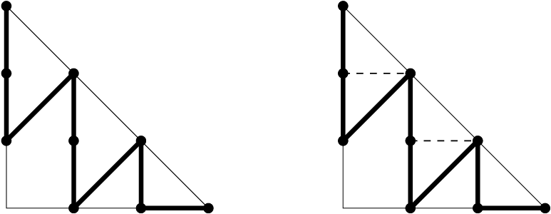
Let us compute $\mu_{+}(\gamma)$ . We have $k=2$ as $\gamma(2)=(0,1)$ is a locally convex vertex of $\Delta_{+}$ . We have $\gamma^{\prime\prime}(2)=(1,3)\notin\Delta_{3}$ and thus $\mu_{+}(\gamma)=\mu_{+}(\gamma^{\prime})$ , since $\operatorname{Area}(T)=\frac{1}{2}$ . Proceeding further we get $\mu_{+}(\gamma)=\mu_{+}(\gamma^{\prime})=\dots=\mu_{+}(\alpha_{+})=1$ .

Let us compute $\mu_{-}(\gamma)$ . We have $k=3$ as $\gamma(3)=(1,2)$ is a locally convex vertex of $\Delta_{-}$ . We have $\gamma^{\prime\prime}(3)=(0,0)$ and $\mu_{-}(\gamma^{\prime\prime})=1$ . To compute $\mu_{-}(\gamma^{\prime})=1$ we note that $\mu_{-}((\gamma^{\prime})^{\prime})=0$ and $\mu_{-}((\gamma^{\prime})^{\prime\prime})=1$ . Thus the full multiplicity of $\gamma$ is 2.

Recall that we fixed an (irrational) linear function $\lambda:\mathbb{R}^{2}\to\mathbb{R}$ and this choice gives us a pair of extremal vertices $p,q\in\Delta$ .

Theorem 2.

The number $N_{\operatorname{trop}}(g,\Delta)$ is equal to the number (counted with multiplicities) of $\lambda$ -increasing lattice paths $[0,s+g-1]\to\Delta$ connecting $p$ and $q$ .

Furthermore, there exists a configuration ${\mathcal{P}}\in\mathbb{R}^{2}$ of $s+g-1$ points in tropical general position such that each $\lambda$ -increasing lattice path encodes a number of tropical curves of genus $g$ and degree $\Delta$ passing via ${\mathcal{P}}$ of total multiplicity $\mu(\gamma)$ . These curves are distinct for distinct paths.

Example 7.3.

Let us compute $N(0,\Delta)=5$ for the polygon $\Delta$ depicted on Figure 17 in two different ways. Using $\lambda(x,y)=-x+\epsilon y$ for a small $\epsilon>0$ we get the left two paths depicted on Figure 17. Using $\lambda(x,y)=x+\epsilon y$ we get the three right paths. The corresponding multiplicities are shown under the path. All other $\lambda$ -increasing paths have zero multiplicity.

In the next two examples we use $\lambda(x,y)=x-\epsilon y$ as the auxiliary linear function.

Example 7.4.

Figure 18 shows a computation of the well-known number $N(0,\Delta_{3})$ . This is the number of rational cubic curves through 8 generic points in ${\mathbb{C}}{\mathbb{P}}^{2}$ .

Example 7.5.

Figure 19 shows a computation of a less well-known number $N(1,\Delta_{4})$ . This is the number of genus 1 quartic curves through 12 generic points in ${\mathbb{C}}{\mathbb{P}}^{2}$ .

7.3. Enumeration of real curves

Let ${\mathcal{Q}}=\{q_{1},\dots,q_{s+g-1}\}\subset(\mathbb{R}^{*})^{2}$ be a configuration of points in general position. We have a total of $N(g,\Delta)$ complex curves of genus $d$ and degree $\Delta$ in $(\mathbb{C}^{*})^{2}$ passing through ${\mathcal{Q}}$ . Some of these curves are defined over $\mathbb{R}$ while others come in complex conjugated pairs.

Definition 7.6.

We define the number $N^{\operatorname{irr}}_{\mathbb{R}}(g,\Delta,{\mathcal{Q}})$ to be the number of irreducible real curves of genus $g$ and degree $\Delta$ passing via ${\mathcal{Q}}$ . Similarly we define the number $N_{\mathbb{R}}(g,\Delta,{\mathcal{Q}})$ to be the number of all real curves of genus $g$ and degree $\Delta$ passing via ${\mathcal{Q}}$ .

Unlike the complex case the numbers $N^{\operatorname{irr}}_{\mathbb{R}}(g,\Delta,{\mathcal{Q}})$ and $N_{\mathbb{R}}(g,\Delta,{\mathcal{Q}})$ do depend on the choice of ${\mathcal{Q}}$ . We have

0\leq N_{\mathbb{R}}(g,\Delta,{\mathcal{Q}})\leq N(g,\Delta)

while $N_{\mathbb{R}}(g,\Delta,{\mathcal{Q}})\equiv N(g,\Delta)\pmod{2}$ and, similarly, $0\leq N^{\operatorname{irr}}_{\mathbb{R}}(g,\Delta,{\mathcal{Q}})\leq N^{\operatorname{irr}}(g,\Delta)$ and $N^{\operatorname{irr}}_{\mathbb{R}}(g,\Delta,{\mathcal{Q}})\equiv N^{\operatorname{irr}}(g,\Delta)\pmod{2}$ .

Tropical geometry allows one to compute $N_{\mathbb{R}}(g,\Delta,{\mathcal{Q}})$ and $N_{\mathbb{R}}(g,\Delta,{\mathcal{Q}})$ for some configurations ${\mathcal{Q}}$ . Note that one can extract a sign sequence $\{\operatorname{Sign}(q_{j})\}_{j=1}^{s-g+1}\subset\mathbb{Z}^{2}_{2}$ from ${\mathcal{Q}}=\{q_{j}\}_{j=1}^{s-g+1}$ by taking the coordinatewise sign. Accordingly we can enhance the tropical configuration data by adding a choice of signs that take values in $\mathbb{Z}^{2}_{2}$ .

Definition 7.7.

A signed tropical configuration of points

{\mathcal{R}}=\{(r_{1},\sigma_{1}),\dots,(r_{s+g-1},\sigma_{s+g-1})\}

is a collection of $s-g+1$ points $r_{j}$ in the tropical plane $\mathbb{R}^{2}$ together with a choice of signs $\sigma_{j}\in\mathbb{Z}^{2}_{2}$ .

We denote with $|{\mathcal{R}}|=\{r_{1},\dots,r_{s+g-1}\}\subset\mathbb{R}^{2}$ the resulting configuration after forgetting the signs.

Suppose that $C$ is a simple tropical curve and is given by an immersion $h:\Gamma\to\mathbb{R}^{2}$ where $\Gamma$ is 3-valent. Let $E$ be an edge of $\Gamma$ of weight $w_{E}$ . Suppose that $(x_{E},y_{E})$ is a primitive integer vector parallel to $E$ . We define the set $S_{E}$ as the quotient of $\mathbb{Z}^{2}_{2}$ by the equivalence relation $(X,Y)\sim(X+w_{E}x_{E},Y+w_{E}y_{E})$ , $X,Y\in\mathbb{Z}_{2}$ . Thus if the weight $w_{E}$ is even then $S_{E}=\mathbb{Z}^{2}_{2}$ but if $w_{E}$ is odd then $S_{E}$ is a 2-element set.

An element $\sigma_{E}\in S_{E}$ is called the phase of $E$ . Every vertex of $\Gamma$ is adjacent to three edges $E_{1},E_{2},E_{3}$ . Their phases $\sigma_{E_{1}},\sigma_{E_{2}},\sigma_{E_{3}}$ are called compatible if there exist representatives $\rho^{j}_{k}\in\mathbb{Z}^{2}_{2}$ , $j,k=1,2,3$ , $j\neq k$ , such that

•

$\rho^{j}_{k}\in\sigma_{E_{k}}$ ,
•

$\rho^{j}_{k}\neq\rho^{j^{\prime}}_{k}$ if $j\neq j^{\prime}$ and the equivalence class $\sigma_{E_{k}}$ contains more than one element,
•

$\rho^{k}_{j}=\rho^{j}_{k}$ .

In other words, once we associate to every phase $\sigma_{E_{k}}$ its two possible representatives in $\mathbb{Z}^{2}_{2}$ (which we choose distinct if there are two elements in $\sigma_{E_{k}}$ and coinciding if $\sigma_{E_{k}}$ is a one-point set) the 6 resulting elements of $\mathbb{Z}^{2}_{2}$ should divide in three pairs of coinciding elements from distinct edges.

Definition 7.8.

A simple real tropical curve (or signed tropical curve) $(C,\{\sigma_{E}\})$ is a simple tropical curve $C$ parameterized by $h:\Gamma\to\mathbb{R}^{2}$ with a choice of the phase $\sigma_{E}\in S_{E}$ for every edge $E\subset\Gamma$ that is compatible at every vertex of $\Gamma$ . We say that $(C,\{\sigma_{E}\})$ passes through a signed configuration ${\mathcal{R}}$ if for every $r_{j}\in|{\mathcal{R}}|$ there exists a (closed) edge $E\subset C$ such that $r_{j}\in E$ and $\sigma_{j}\in\sigma_{E}$ .

Remark 7.9.

Signed tropical configuration and real tropical curves both can be viewed as 0- and 1-dimensional real tropical varieties in $\mathbb{R}^{2}$ respectively.

Suppose that ${\mathcal{R}}$ is such that $|{\mathcal{R}}|\subset\mathbb{R}^{2}$ is a configuration of $n$ points in general position. Let $(C,\{\sigma_{E}\})$ be a real tropical curve passing through a signed configuration ${\mathcal{R}}$ . Suppose that $x+g-1=n$ , where $x$ is the number of ends of $C$ and $g$ is the genus of $C$ .

Definition 7.10.

The multiplicity $\mu(C,\{\sigma_{E}\},{\mathcal{R}})$ is $2^{N^{\operatorname{even}}}$ , where $N^{\operatorname{even}}$ is twice the number of edges of $\Gamma$ of even weight that contain points from $|{\mathcal{R}}|$ plus the number of the remaining edges of $\Gamma$ of even weight.

A real tropical curve $(C,\{\sigma_{E}\})$ is called irreducible if the tropical curve $C$ is irreducible. Otherwise, it is called reducible.

Definition 7.11.

We define the number $N^{\operatorname{irr}}_{\operatorname{trop},{\mathbb{R}}}(g,\Delta,{\mathcal{R}})$ to be the number of real irreducible tropical curves $(C,\{\sigma_{E}\})$ of genus $g$ and degree $\Delta$ passing via ${\mathcal{R}}$ counted with multiplicities $\mu(C,\{\sigma_{E}\},{\mathcal{R}})$ . Similarly we define the number $N_{\operatorname{trop},{\mathbb{R}}}(g,\Delta,{\mathcal{R}})$ to be the number of all real tropical curves of genus $g$ and degree $\Delta$ passing via ${\mathcal{R}}$ (again, counted with multiplicities $\mu(C,\{\sigma_{E}\},{\mathcal{R}})$ ).

Theorem 3.

Suppose that ${\mathcal{R}}$ is a signed configuration of $s+g-1$ points in tropically general position. Then there exists a configuration ${\mathcal{Q}}\subset(\mathbb{R}^{*})^{2}$ of $s+g-1$ real points in general position such that $N^{\operatorname{irr}}_{\mathbb{R}}(g,\Delta,{\mathcal{Q}})=N^{\operatorname{irr}}_{\operatorname{trop},{\mathbb{R}}}(g,\Delta,{\mathcal{R}})$ and $N_{\mathbb{R}}(g,\Delta,{\mathcal{Q}})=N_{\operatorname{trop},{\mathbb{R}}}(g,\Delta,{\mathcal{R}})$ .

Furthermore, for every real tropical curve $(C,\{\sigma_{E}\})$ of genus $g$ and degree $\Delta$ passing through ${\mathcal{R}}$ we have $\mu(C,\{\sigma_{E}\},{\mathcal{R}})$ distinct real curves of genus $g$ and degree $\Delta$ passing through ${\mathcal{Q}}$ . These curves are distinct for distinct $C$ and are irreducible if $C$ is irreducible.

Our next goal is to define the real multiplicity $\mu_{\mathbb{R}}(C,{\mathcal{R}})$ of a tropical curve $C$ passing through a signed configuration ${\mathcal{R}}$ in a way to include all signed tropical curves $(C,\{\sigma_{E}\})$ with the same $C$ with corresponding multiplicities. The multiplicity $\mu_{\mathbb{R}}(C,{\mathcal{R}})$ depends only on $C$ , $|{\mathcal{R}}|$ and the equivalence class $\sigma_{E}\in S_{E}$ of the sign $\sigma_{j}$ for every point $r_{j}\in{\mathcal{R}}$ contained in the edge $E$ . (Recall that since $|{\mathcal{R}}|\subset\mathbb{R}^{2}$ is tropically in general position, the points $r_{j}$ are disjoint from the vertices of $C$ .)

Let $h:\Gamma\to\mathbb{R}^{2}$ be a tropical curve of genus $g$ and degree $\Delta$ passing through $|{\mathcal{R}}|$ . Recall that by Lemma 4.20 each component of $\Gamma\smallsetminus h^{-1}(|{\mathcal{R}}|)$ is a tree with a single end at infinity (see Figure 12).

We define the real tropical multiplicity $\mu_{\mathbb{R}}(T,{\mathcal{R}})$ of each component $T$ of $\Gamma\smallsetminus h^{-1}(|{\mathcal{R}}|)$ inductively. Let $A$ and $B$ be two 1-valent vertices of $T$ corresponding to marked points $r_{a}$ and $r_{b}$ such that the edges adjacent to $A$ and $B$ meet at a 3-valent vertex $C$ (see Figure 20).

Form a new tree $T^{\prime}$ by removing the edges $[A,C]$ and $[B,C]$ from $T$ . The number of 1-valent vertices of $T^{\prime}$ is less by one ( $C$ becomes a new 1-valent vertex while $A$ and $B$ disappear). By the induction assumption the real multiplicity of $T^{\prime}$ is already defined for any choice of signs. All the finite 1-valent vertices of $T^{\prime}$ except for $C$ have their signs induced from the signs of $T$ . To completely equip $T^{\prime}$ with the signs we have to define the sign $\sigma_{d}$ at the edge $[C,D]$ .

Suppose that $(x_{a},y_{a})$ and $(x_{b},y_{b})$ are primitive integer vectors parallel to $[A,C]$ and $[B,C]$ respectively. Suppose that the signs of $[A,C]$ and $[B,C]$ are $\sigma_{a}$ and $\sigma_{b}$ . Suppose that $[C,D]$ is the third edge adjacent to $C$ . Let $S_{a}$ , $S_{b}$ , $S_{d}$ be the set of equivalence classes of signs corresponding to $[A,C]$ , $[B,C]$ and $[C,D]$ . Let $w_{a},w_{b},w_{d}$ be their weights.

Definition 7.12.

The sign at $C$ and the real multiplicity of $T$ are defined according to the following inductive rules. If $T$ does not have a 3-valent vertex (i.e. $T$ is homeomorphic to $\mathbb{R}$ ) then $\mu_{R}(T)=1$ .

•

Suppose that $w_{a}\equiv w_{b}\equiv 1\pmod{2}$ and $(x_{a},y_{a})\equiv(x_{b},y_{b})\pmod{2}$ . In this case we have $S_{a}=S_{b}$ so the signs $\sigma_{a}$ and $\sigma_{b}$ take values in the same set. Note that $w_{d}\equiv 0\pmod{2}$ in this case. The sign $\sigma_{d}$ on such edge takes values in $S_{d}=\mathbb{Z}^{2}_{2}$ . If $\sigma_{a}=\sigma_{b}$ then this sign can be presented by two distinct equivalent elements $\sigma^{+}_{d},\sigma^{-}_{d}\in\mathbb{Z}^{2}_{2}$ . Let $T^{\prime}_{+}$ and $T^{\prime}_{-}$ be the trees equipped with the corresponding signs. We set

(12) $\mu_{\mathbb{R}}(T)=\mu_{\mathbb{R}}(T^{\prime}_{+})+\mu_{\mathbb{R}}(T^{\prime}_{-}).$

If $\sigma_{a}\neq\sigma_{b}$ we set $\mu_{\mathbb{R}}(T)=0$ .
•

Suppose that $w_{a}\equiv w_{b}\equiv 1\pmod{2}$ and $(x_{a},y_{a})\not\equiv(x_{b},y_{b})\pmod{2}$ . In this case $w_{d}\equiv 1\pmod{2}$ and the three sets $S_{a},S_{b},S_{d}$ are all distinct. The sign $\sigma_{d}\in S_{d}$ is uniquely determined by the condition that its equivalence class has common elements both with the equivalence class $\sigma_{a}$ and with the equivalence class $\sigma_{b}$ . Let $T^{\prime}$ be the tree equipped with this sign. We set

(13) $\mu_{\mathbb{R}}(T)=\mu_{\mathbb{R}}(T^{\prime}).$
•

Suppose that one of the weights $w_{a}$ and $w_{b}$ is odd and the other is even. We may suppose without the loss of generality that $w_{a}\equiv 1\pmod{2}$ and $w_{b}\equiv 0\pmod{2}$ . In this case we have $w_{d}\equiv 1\pmod{2}$ and $S_{a}=S_{d}$ while $S_{b}=\mathbb{Z}^{2}_{2}$ . If the equivalence class $\sigma_{a}$ contains $\sigma_{b}$ we set $\sigma_{d}=\sigma_{a}$ and

(14) $\mu_{\mathbb{R}}(T)=2\mu_{\mathbb{R}}(T^{\prime}),$

where $T^{\prime}$ is equipped with the sign $\sigma_{d}$ at $[C,D]$ . If the equivalence class $\sigma_{a}$ does not contain $\sigma_{b}$ we set $\mu_{\mathbb{R}}(T)=0$ .
•

Suppose that $w_{a}\equiv w_{b}\equiv 0\pmod{2}$ . Then $w_{d}$ is even and $S_{a}=S_{b}=S_{d}=\mathbb{Z}^{2}_{2}$ . If $\sigma_{a}=\sigma_{b}$ we set $\sigma_{d}=\sigma_{a}$ and

(15) $\mu_{\mathbb{R}}(T)=4\mu_{\mathbb{R}}(T^{\prime}),$

where $T^{\prime}$ is equipped with the sign $\sigma_{d}$ at $[C,D]$ . If $\sigma_{a}\neq\sigma_{b}$ we set $\mu_{\mathbb{R}}(T)=0$ .

Let ${\mathcal{R}}$ be a signed configuration of $s+g-1$ points and $h:\Gamma\to\mathbb{R}^{2}$ be a tropical curve $C=h(\Gamma)$ of genus $g$ and degree $\Delta$ passing via $|{\mathcal{R}}|$ . The real multiplicity of a tropical curve passing through the signed configuration ${\mathcal{R}}$ is the product

\mu_{\mathbb{R}}(C,{\mathcal{R}})=\prod\limits_{T}\mu_{\mathbb{R}}(T),

where $T$ runs over all the components of $\Gamma\smallsetminus h^{-1}(|{\mathcal{R}}|)$ .

Proposition 7.13.

The real multiplicity $\mu_{\mathbb{R}}(C,{\mathcal{R}})$ is never greater than and has the same parity as the multiplicity of $C$ from Definition 4.15.

Proof.

The proposition follows directly from Definition 7.12 by induction. The multiplicity of a three-valent vertex is odd if and only if all three adjacent edges have odd weights. This multiplicity is at least 2 if one of the adjacent edges has even weight. This multiplicity is at least 4 if all three adjacent edges have even weights. ∎

Proposition 7.14.

The multiplicity $\mu_{\mathbb{R}}(C,{\mathcal{R}})$ equals to the sum of multiplicities $\mu(C,\{\sigma_{E}\},{\mathcal{R}})$ for all real tropical curves $(C,\{\sigma_{E}\})$ with the same $C$ .

Proof.

The proposition follows from induction. In all except for the first case of Definition 7.12 we have a unique choice for the phase of $[C,D]$ compatible at $C$ . In the first case we have two choices that are accounted in (12). ∎

Corollary 7.15.

The number $N^{\operatorname{irr}}_{\operatorname{trop},{\mathbb{R}}}(g,\Delta,{\mathcal{R}})$ is equal to the sum of $\mu_{\mathbb{R}}(C,{\mathcal{R}})$ over all irreducible tropical curves $C$ passing through $|{\mathcal{R}}|$ .

The number $N_{\operatorname{trop},{\mathbb{R}}}(g,\Delta,{\mathcal{R}})$ is equal to the sum of $\mu_{\mathbb{R}}(C,{\mathcal{R}})$ over all tropical curves $C$ passing through $|{\mathcal{R}}|$ .

Example 7.16.

Let us choose the signs of ${\mathcal{R}}$ so that every $\sigma_{j}$ contains $(+,+)\in\mathbb{Z}^{2}_{2}$ in its equivalence class. Let $g=0$ and $\Delta$ be the quadrilateral whose vertices are $(0,0)$ , $(1,0)$ , $(0,1)$ and $(2,2)$ as in Example 4.14. Then we have $N_{\operatorname{trop},{\mathbb{R}}}(g,\Delta,{\mathcal{R}})=3$ for the configuration of 3 points from Figure 9 and $N_{\operatorname{trop},{\mathbb{R}}}(g,\Delta,{\mathcal{R}})=5$ for the configuration of 3 points from Figure 10.

For other choices of signs of ${\mathcal{R}}$ we can get $N_{\operatorname{trop},{\mathbb{R}}}(g,\Delta,{\mathcal{R}})=1$ for Figure 10 while $N_{\operatorname{trop},{\mathbb{R}}}(g,\Delta,{\mathcal{R}})=3$ for Figure 9 for any sign choices.

7.4. Counting of real curves by lattice paths

Theorem 2 can be modified to give the relevant count of real curves. In order to do this we need to define the real multiplicity of a lattice path $\gamma:[0,n]\to\Delta$ connecting the vertices $p$ and $q$ once $\gamma$ is equipped with signs.

Suppose $\gamma(j)-\gamma(j-1)=(y_{j},x_{j})\in\mathbb{Z}^{2}$ , $j=1,\dots,n$ . Let $w_{j}\in\mathbb{N}$ be the GCD of $y_{j}$ and $x_{j}$ . Similarly to the previous subsection we define $S_{j}$ to be the set obtained from $\mathbb{Z}^{2}_{2}$ by taking the quotient under the equivalence relation $(X,Y)\sim(X+x_{j},Y+y_{j})$ , $X,Y\in\mathbb{Z}_{2}$ . Let

\sigma=\{\sigma_{j}\}_{j=1}^{n},\ \sigma_{j}\in S_{j}

be any choice of signs.

We set

(16)

\mu^{\mathbb{R}}_{\pm}(\gamma,\sigma)=a(T)\mu^{\mathbb{R}}_{\pm}(\gamma^{\prime},\sigma^{\prime})+\mu^{\mathbb{R}}_{\pm}(\gamma^{\prime\prime},\sigma^{\prime\prime}).

The definition of the new paths $\gamma^{\prime}$ , $\gamma^{\prime\prime}$ and the triangle $T$ is the same as in subsection 15. The sign sequence for $\gamma^{\prime\prime}$ is $\sigma^{\prime\prime}_{j}=\sigma_{j},j\neq k,k+1$ , $\sigma^{\prime\prime}_{k}=\sigma_{k+1}$ , $\sigma^{\prime\prime}_{k+1}=\sigma_{k}$ . The sign sequence for $\gamma^{\prime}$ is $\sigma^{\prime}_{j}=\sigma_{j},j<k$ , $\sigma^{\prime}_{j}=\sigma_{j+1},j>k$ . We define the sign $\sigma^{\prime}_{k}$ and the function $a(T)$ (in a way similar to Definition 7.12) as follows.

•

If all sides of $T$ are odd we set $a(T)=1$ and define the sign $\sigma^{\prime}_{k}$ (up to the equivalence) by the condition that the three equivalence classes of $\sigma_{k}$ , $\sigma_{k+1}$ and $\sigma^{\prime}_{k}$ do not share a common element.
•

If all sides of $T$ are even we set $a(T)=0$ if $\sigma_{k-1}\neq\sigma_{k}$ . In this case we can ignore $\gamma^{\prime}$ (and its sequence of signs). We set $a(T)=4$ if $\sigma_{k}=\sigma_{k+1}$ . In this case we define $\sigma^{\prime}_{k}=\sigma_{k}=\sigma_{k+1}$ .
•

Otherwise we set $a(T)=0$ if the equivalence classes of $\sigma_{k}$ and $\sigma_{k+1}$ do not have a common element. We set $a(T)=2$ if they do. In the latter case we define the equivalence class of $\sigma^{\prime}_{k}$ by the condition that $\sigma_{k}$ , $\sigma_{k+1}$ and $\sigma^{\prime}_{k}$ have a common element. There is one exception to this rule. If the even side is $\gamma(k+1)-\gamma(k-1)$ then there are two choices for $\sigma^{\prime}_{k}$ satisfying the above condition. In this case we replace $a(T)\mu^{\mathbb{R}}_{\pm}(\gamma^{\prime})$ in (16) by the sum of the two multiplicities of $\gamma^{\prime}$ equipped with the two allowable choices for $\sigma^{\prime}_{k}$ (note that this agrees with $a(T)=2$ in this case).

Similar to subsection 15 we define $\mu^{\mathbb{R}}_{\pm}(\alpha_{\pm})=1$ and $\mu^{\mathbb{R}}(\gamma,\sigma)=\mu^{\mathbb{R}}_{+}(\gamma,\sigma)\mu^{\mathbb{R}}_{-}(\gamma,\sigma)$ . As before $\lambda:\mathbb{R}^{2}\to\mathbb{R}$ is a linear map injective on $\mathbb{Z}^{2}$ and $p$ and $q$ are the extrema of $\lambda|_{\Delta}$ .

Theorem 4.

For any choice of $\sigma_{j}\in\mathbb{Z}^{2}_{2}$ , $j=1,\dots,s+g-1$ there exists a configuration of $s+g-1$ of generic points in the respective quadrants such that the number of real curves among the $N(g,\Delta)$ relevant complex curves is equal to the number of $\lambda$ -increasing lattice paths $\gamma:[0,s+g-1]\to\Delta$ connecting $p$ and $q$ counted with multiplicities $\mu^{\mathbb{R}}$ .

Furthermore, each $\lambda$ -increasing lattice path encodes a number of tropical curves of genus $g$ and degree $\Delta$ passing via ${\mathcal{R}}$ of total real multiplicity $\mu^{\mathbb{R}}(\gamma,\sigma)$ . These curves are distinct for distinct paths.

Example 7.17.

Here we use the choice $\sigma_{j}=(+,+)$ so all the points $z_{j}$ are in the positive quadrant $(\mathbb{R}_{>0})^{2}\subset(\mathbb{R}^{*})^{2}$ . The first count of the number $N(0,\Delta)$ from Example 7.3 gives a configuration of 3 real points with 5 real curves. The second count gives a configuration with 3 real curves as the real multiplicity of the last path is 1. Note also that the second path on Figure 17 changes its real multiplicity if we reverse its direction.

Example 7.4 gives a configuration of 9 generic points in ${\mathbb{R}}{\mathbb{P}}^{2}$ with all 12 nodal cubics through them real. Example 7.5 gives a configuration of 12 generic points in ${\mathbb{R}}{\mathbb{P}}^{2}$ with 217 out of the 225 quartics of genus 1 real. The path in the middle of Figure 19 has multiplicity 9 but real multiplicity 1. A similar computation shows that there exists a configuration of 11 generic points in ${\mathbb{R}}{\mathbb{P}}^{2}$ such that 564 out of the 620 irreducible quartic through them are real.

7.5. Different types of real nodes and the Welschinger invariant

Let $V\subset(\mathbb{C}^{*})^{2}$ be a curve defined over $\mathbb{R}$ . In other words it is a curve invariant with respect to the involution of complex conjugation. Suppose that $V$ is nodal, i.e. all singularities of $V$ are ordinary double points (nodes).

There are three types of nodes of $V$ :

•

Hyperbolic. These are the real nodes that locally are intersections of a pair of real branches. Such nodes are given by equation $z^{2}-w^{2}=0$ for a choice of local real coordinates $(z,w)$ .
•

Elliptic. These are the real nodes that locally are intersections of a pair of imaginary branches. Such nodes are given by equation $z^{2}+w^{2}=0$ for a choice of local real coordinates $(z,w)$ .
•

Imaginary. These are nodes at non-real points of $V$ . Such nodes come in complex conjugate pairs.

This distinction was used in [30] in order to get a real curve counting invariant with respect to the initial configuration ${\mathcal{P}}\subset(\mathbb{R}^{*})^{2}$ . Indeed, let us modify the real enumerative problem from Definition 7.6 in the following way. Let $V\subset(\mathbb{C}^{*})^{2}$ be a real nodal curve. Let $e(V)$ be the number of real elliptic nodes of $V$ . We prescribe to $V$ the sign equal to $(-1)^{e(V)}$ . As usual we fix a genus $g$ , a degree $\Delta$ and a configuration ${\mathcal{P}}\in(\mathbb{R}^{*})^{2}$ of $s+g-1$ points in general position.

Definition 7.18 (see [30]).

We define the number $N^{\operatorname{irr}}_{\mathbb{R},W}(g,\Delta,{\mathcal{P}})$ to be the number of irreducible real curves of genus $g$ and degree $\Delta$ passing via ${\mathcal{P}}$ counted with signs. Similarly we define the number $N_{\mathbb{R},W}(g,\Delta,{\mathcal{P}})$ to be the number of all real curves of genus $g$ and degree $\Delta$ passing via ${\mathcal{P}}$ counted with signs.

Theorem 5 (Welschinger [30]).

If $g=0$ and $\mathbb{C}T_{\Delta}$ is smooth then the number $N^{\operatorname{irr}}_{\mathbb{R},W}(g,\Delta,{\mathcal{P}})$ does not depend on the choice of ${\mathcal{P}}$ .

Theorem 3 can be modified to compute $N^{\operatorname{irr}}_{\mathbb{R},W}(g,\Delta,{\mathcal{P}})$ and $N_{\mathbb{R},W}(g,\Delta,{\mathcal{P}})$ for an arbitrary $g$ , in particular, in the invariant situation $g=0$ .

Let $C\subset\mathbb{R}^{2}$ be a simple tropical curve. Recall that Definition 2.16 assigns a multiplicity $\operatorname{mult}_{V}(C)$ to every 3-valent vertex $V\in C$ .

Definition 7.19.

We define

\operatorname{mult}_{V}^{\mathbb{R},W}(C)=(-1)^{\frac{\operatorname{mult}_{V}(C)-1}{2}}

if $\operatorname{mult}_{V}(C)$ is odd and $\operatorname{mult}_{V}^{\mathbb{R},W}(C)=0$ if $\operatorname{mult}_{V}(C)$ is even.

The tropical Welschinger sign $\operatorname{mult}^{\mathbb{R},W}(C)$ is the product of $\operatorname{mult}_{V}^{\mathbb{R},W}(C)$ over all 3-valent vertices of $C$ .

As usual let us fix a genus $g$ , a degree $\Delta$ and a configuration ${\mathcal{R}}\subset\mathbb{R}^{2}$ of $s+g-1$ points in tropically general position. Define $N^{\operatorname{irr}}_{\operatorname{trop},{\mathbb{R}},W}(g,\Delta,{\mathcal{R}})$ to be the number of irreducible tropical curves of genus $g$ and degree $\Delta$ passing via ${\mathcal{R}}$ counted with the Welschinger sign. In a similar way define $N_{\operatorname{trop},{\mathbb{R}},W}(g,\Delta,{\mathcal{R}})$ to be the number of all tropical curves of genus $g$ and degree $\Delta$ passing via ${\mathcal{R}}$ counted with the Welschinger sign.

Theorem 6.

Suppose that ${\mathcal{R}}\subset\mathbb{R}^{2}$ is a configuration of $s+g-1$ points in tropically general position. Then there exists a configuration ${\mathcal{P}}\subset(\mathbb{R}^{*})^{2}$ of $s+g-1$ real points in general position such that

N^{\operatorname{irr}}_{\mathbb{R},W}(g,\Delta,{\mathcal{P}})=N^{\operatorname{irr}}_{\operatorname{trop},{\mathbb{R}},W}(g,\Delta,{\mathcal{R}})

and

N_{\mathbb{R},W}(g,\Delta,{\mathcal{P}})=N_{\operatorname{trop},{\mathbb{R}},W}(g,\Delta,{\mathcal{R}}).

Furthermore, for every tropical curve $C$ of genus $g$ and degree $\Delta$ passing through ${\mathcal{R}}$ we have a number of distinct real curves of genus $g$ and degree $\Delta$ passing through ${\mathcal{P}}$ with the total sum equal to the Welschinger sign of $C$ . These curves are distinct for distinct $C$ and are irreducible if $C$ is irreducible.

Example 7.20.

Let $g=0$ and $\Delta$ be the quadrilateral with vertices $(0,0)$ , $(1,0)$ , $(0,1)$ and $(2,2)$ . In Figure 9 we have 3 real curves, two of them have the sign $+1$ and one has the sign $-1$ . In Figure 10 we have 2 real curves, one of them has the sign $+1$ and one has the sign $0$ . In both cases we have $N_{\operatorname{trop},{\mathbb{R}},W}(g,\Delta,{\mathcal{R}})=1$ .

Theorem 2 can be adjusted to compute $N_{\operatorname{trop},{\mathbb{R}},W}(g,\Delta,{\mathcal{R}})$ by lattice paths. Let $\gamma:[0,n]\to\Delta$ be a lattice path connecting the vertices $p$ and $q$ of $\Delta$ . Let us introduce the multiplicity $\nu^{\mathbb{R}}$ inductively, in a manner similar to our definition of the multiplicity $\mu(\gamma)$ . Namely we set $\nu^{\mathbb{R}}(\gamma)=\nu_{+}^{\mathbb{R}}(\gamma)\nu_{-}^{\mathbb{R}}(\gamma)$ . To define $\nu_{\pm}^{\mathbb{R}}(\gamma)$ we repeat the definition of $\mu_{\pm}(\gamma)$ but replace (11) with

\nu^{\mathbb{R}}_{\pm}(\gamma)=b(T)\nu^{\mathbb{R}}_{\pm}(\gamma^{\prime})+\nu^{\mathbb{R}}_{\pm}(\gamma^{\prime\prime}).

Here we define $b(T)=0$ if at least one side of $T$ is even and $b(T)=(-1)^{\#(\operatorname{Int}T\cap\mathbb{Z}^{2})}$ otherwise. The paths $\gamma^{\prime}$ , $\gamma^{\prime\prime}$ and the triangle $T$ are the same as in the inductive definition of $\mu_{\pm}$ .

Theorem 7.

For any choice of an irrational linear map $\lambda:\mathbb{R}^{2}\to\mathbb{R}$ there exists a configuration ${\mathcal{P}}$ of $s+g-1$ of generic points in $(\mathbb{R}^{*})^{2}$ such that the number of (not necessarily irreducible) real curves of genus $g$ and degree $\Delta$ passing through ${\mathcal{P}}$ counted with the tropical Welschinger sign is equal to the number of $\lambda$ -increasing lattice paths $\gamma:[0,s+g-1]\to\Delta$ connecting $p$ and $q$ counted with multiplicities $\nu^{\mathbb{R}}$ .

Furthermore, there exists a configuration ${\mathcal{R}}\in\mathbb{R}^{2}$ of $s+g-1$ points in tropical general position such that each $\lambda$ -increasing lattice path encodes a number of tropical curves of genus $g$ and degree $\Delta$ passing via ${\mathcal{R}}$ with the sum of signs equal to $\nu^{\mathbb{R}}(\gamma)$ . These curves are distinct for distinct paths.

Example 7.21.

In example 7.3 we have $N_{\mathbb{R},W}(0,\Delta,{\mathcal{P}})=1$ for some choice of ${\mathcal{P}}$ . In example 7.4 we have $N_{\mathbb{R},W}(0,\Delta_{3},{\mathcal{P}})=8$ for some choice of ${\mathcal{P}}$ . In example 7.5 we have $N_{\mathbb{R},W}(1,\Delta_{4},{\mathcal{P}})=93$ for some choice of ${\mathcal{P}}$ . In all these examples we have $N^{\operatorname{irr}}_{\mathbb{R},W}=N_{\mathbb{R},W}$ as there are no reducible curves of these genera and degree. Note that by Theorem 5 the number $N^{\operatorname{irr}}_{\mathbb{R},W}(0,\Delta_{3},{\mathcal{P}})=8$ does not depend on the choice of ${\mathcal{P}}$ .

The following observation is due to Itenberg, Kharlamov and Shustin [9]. If $\lambda(x,y)=x-\epsilon y$ and $\Delta=\Delta_{d}$ or $\Delta=[0,d_{1}]\times[0,d_{2}]$ then $\nu^{\mathbb{R}}(\gamma)\geq 0$ for any $\lambda$ -increasing path $\gamma$ and, furthermore, any tropical curve encoded by $\gamma$ by Theorem 7 has a non-negative tropical Welschinger sign. It is easy to show that there exist $\lambda$ -increasing paths that encode irreducible tropical curves of non-zero tropical Welschinger signs. We get the following corollary for any $d,d_{1},d_{2}\in\mathbb{N}$ .

Corollary 8.

For any generic configuration ${\mathcal{P}}\subset{\mathbb{R}}{\mathbb{P}}^{2}$ of $3d-1$ points there exists an irreducible rational curve $V\subset{\mathbb{R}}{\mathbb{P}}^{2}$ of degree $d$ passing through ${\mathcal{P}}$ .

For any generic configuration ${\mathcal{P}}\subset{\mathbb{R}}{\mathbb{P}}^{1}\times{\mathbb{R}}{\mathbb{P}}^{1}$ of $2d_{1}+2d_{2}-1$ points there exists an irreducible rational curve $V\subset{\mathbb{R}}{\mathbb{P}}^{1}\times{\mathbb{R}}{\mathbb{P}}^{1}$ of bidegree $(d_{1},d_{2})$ passing through ${\mathcal{P}}$ .

With the help of Theorem 7 Itenberg, Kharlamov and Shustin in [9] have obtained a non-trivial lower bound for the number of such rational curves. In particular, they have shown that for any generic configuration ${\mathcal{P}}$ of $3d-1$ points in ${\mathbb{R}}{\mathbb{P}}^{2}$ there exists at least $\frac{d!}{2}$ rational curves of degree $d$ passing via ${\mathcal{P}}$ .

8. Proof of the main theorems

8.1. Complex amoebas in $\mathbb{R}^{2}$ and the key lemma

Let ${\mathcal{Q}}=\{q_{1},\dots,q_{n}\}\subset(\mathbb{C}^{*})^{2}$ be generic points in the sense of Proposition 5.2 (i.e. generic classically). Suppose in addition that the points

p_{1}=\operatorname{Log}(q_{1}),\dots,p_{n}=\operatorname{Log}(q_{n})\in\mathbb{R}^{2}

are in general position tropically. Denote ${\mathcal{P}}=\{p_{1},\dots,p_{n}\}\subset\mathbb{R}^{2}$ . Recall that we fix a Newton polygon $\Delta\subset\mathbb{R}^{2}$ and a genus $g\in\mathbb{N}$ . There are $N(g,\Delta)$ holomorphic curves passing through ${\mathcal{Q}}$ as long as $n=s+g-1$ . By Proposition 4.13 there are finitely many tropical curves

(17)

C_{1},\dots,C_{m}\subset\mathbb{R}^{2}

of genus $g$ with the Newton polygon $\Delta$ and passing through ${\mathcal{P}}$ . Note that $m$ depends on the choice of the points $x_{j}$ (unlike the number $N_{\operatorname{trop}}(g,\Delta)\geq m$ for which we are proving invariance).

Proposition 8.1.

For generic $t$ we have $N(g,\Delta)$ $J_{t}$ -holomorphic curves passing through ${\mathcal{Q}}$ .

Proof.

Indeed, this number equals to the number of holomorphic (i.e. $J_{e}$ -holomorphic) curves through the points $H_{t}(p_{1}),\dots,H_{t}(p_{n})$ . (These points are in general position for generic $t$ since they are for $t=e$ .) ∎

Let $\mathcal{N}_{\epsilon}(C_{j})$ be the $\epsilon$ -neighborhood (in the sense of the standard Euclidean metric on $\mathbb{R}^{2}$ ) of $C_{j}$ for $\epsilon>0$ . Recall (see [6]) that the amoeba of a curve $V\subset(\mathbb{C}^{*})^{2}$ is its image

\mathcal{A}=\operatorname{Log}(V)\subset\mathbb{R}^{2}.

Note that if $V$ is a $J_{t}$ -holomorphic curve then $\operatorname{Log}(V)$ can be obtained from the amoeba of some holomorphic curve by the $\log(t)$ -contraction. This allows us to speak of the Newton polygons of $J_{t}$ -holomorphic curves.

Proposition 8.2.

If $V$ is a $J_{t}$ -holomorphic curve whose Newton polygon is $\Delta$ then its amoeba $\mathcal{A}=\operatorname{Log}(V)$ contains a tropical curve $C$ with the same Newton polygon $\Delta$ .

Proof.

If $t=e$ , i.e. $C$ is holomorphic with respect to the standard holomorphic structure, then the statement follows from the theorem of Passare and Rullgård [19]. Recall (see [19]) that if $V$ is a complex curve defined by a polynomial $f(z,w)=\sum\limits_{j,k}a_{j,k}z^{j}w^{k}$ then the spine of its amoeba $\mathcal{A}$ is a tropical curve defined by a tropical polynomial $N^{\infty}_{f}(x,y)=``\sum\limits_{j,k}b_{j,k}x^{j}y^{k}",$ where

b_{j,k}=\frac{1}{(2\pi i)^{2}}\int\limits_{\operatorname{Log}^{-1}(r)}\log|f(z,w)|\frac{dz}{z}\frac{dw}{w}

and $r\in\mathbb{R}^{2}\smallsetminus\mathcal{A}$ is any point such that its index is $(j,k)$ . If there are no points in $\mathbb{R}^{2}\smallsetminus\mathcal{A}$ of index $(j,k)$ then the monomial $x^{j}y^{k}$ is omitted from $N^{\infty}_{f}$ .

It is shown in [19] that the tropical hypersurface defined by $N^{\infty}_{f}$ is contained in $\mathcal{A}$ . Clearly, the Newton polygon of $N^{\infty}_{f}$ is $\Delta$ . To finish the proof we note that the image of a tropical curve under a homothety is tropical with the same Newton polygon. ∎

With the help of Proposition 8.1 Theorem 1 follows from the following two lemmas.

Lemma 8.3.

For any $\epsilon>0$ there exists $T>1$ such that if $t>T$ and $V$ is a $J_{t}$ -holomorphic curve of genus $g$ , degree $\Delta$ and passing through ${\mathcal{Q}}$ then its amoeba $\operatorname{Log}(V)$ is contained in the $\epsilon$ -neighborhood $\mathcal{N}_{\epsilon}(C_{j})$ of $C_{j}$ for some $j=1,\dots,m$ .

Lemma 8.4.

For a sufficiently small $\epsilon>0$ and a sufficiently large $t>0$ the multiplicity $\operatorname{mult}(C_{j})$ of each $C_{j}$ from (17) (see Definition 4.15) is equal to the number of the $J_{t}$ -holomorphic curves $V$ of genus $g$ and degree $\Delta$ passing through ${\mathcal{Q}}$ and such that $\operatorname{Log}(V)$ is contained in $\mathcal{N}_{\epsilon}(C_{j})$ . Furthermore, if $C_{j}$ is irreducible then any $J_{t}$ -holomorphic curve $V$ of genus $g$ and degree $\Delta$ passing through ${\mathcal{Q}}$ with $\operatorname{Log}(V)\subset\mathcal{N}_{\epsilon}(C_{j})$ is irreducible while if $C_{j}$ is reducible than any such curve $V$ is reducible.

8.2. Proof of Lemma 8.3

A holomorphic curve $V\subset(\mathbb{C}^{*})^{2}$ is given by a polynomial

F(z_{1},z_{2})=\sum\limits_{(j,k)\in\Delta}a_{j,k}z_{1}^{j}z_{2}^{k}.

To a curve $V\subset(\mathbb{C}^{*})^{2}$ we associate its tropicalization $V^{\operatorname{trop}}\subset\mathbb{R}^{2}$ given by the tropical polynomial

F^{\operatorname{trop}}(y_{1},y_{2})=\max\limits_{(j,k)\in\Delta}(jy_{1}+ky_{2}+\log|a_{j,k}|).

Lemma 8.5.

The amoeba $\operatorname{Log}(V)$ is contained in the $\delta$ -neighborhood of $V^{\operatorname{trop}}$ (with respect to the Euclidean metric in $\mathbb{R}^{2}$ ), where

\delta=\log(\#(\Delta\cap\mathbb{Z}^{2})-1).

Proof.

Suppose that $(y_{1},y_{2})$ is not contained in the $\delta$ -neighborhood of $V^{\operatorname{trop}}$ . Then there exists $(j^{\prime},k^{\prime})$ such that

(18)

j^{\prime}y_{1}+k^{\prime}y_{2}+\log|a_{j^{\prime},k^{\prime}}|>jy_{1}+ky_{2}+\log|a_{j,k}|+\delta

for any $(j,k)\neq(j^{\prime},k^{\prime})$ . Indeed, the distance from $(y_{1},y_{2})$ to the line $j^{\prime}y_{1}+k^{\prime}y_{2}+\log|a_{j^{\prime},k^{\prime}}|=jy_{1}+ky_{2}+\log|a_{j,k}|$ is greater than $\delta$ by the hypothesis and the norm of the gradient of the function $(j-j^{\prime})y_{1}+(k-k^{\prime})y_{2}$ is at least 1 (as $j,j^{\prime},k,k^{\prime}$ are all integers).

Suppose that $(z_{1},z_{2})\in V\subset(\mathbb{C}^{*})^{2}$ is such that $\operatorname{Log}(z_{1},z_{2})=(y_{1},y_{2})$ . Since $\sum\limits_{(j,k)\in\Delta}a_{j,k}z_{1}^{j}z_{2}^{k}=0$ the triangle inequality implies that

|a_{j^{\prime},k^{\prime}}z_{1}^{j^{\prime}}z_{2}^{k^{\prime}}|\leq|\sum\limits_{(j,k)\neq(j^{\prime},k^{\prime})}a_{j,k}z_{1}^{j}z_{2}^{k}|.

Let us apply $\log$ to both sides of this inequality:

j^{\prime}y_{1}+k^{\prime}y_{2}+\log|a_{j^{\prime},k^{\prime}}|=\log|a_{j^{\prime},k^{\prime}}z_{1}^{j^{\prime}}z_{2}^{k^{\prime}}|\leq

\log|\sum\limits_{(j,k)\neq(j^{\prime},k^{\prime})}a_{j,k}z_{1}^{j}z_{2}^{k}|\leq\log((\#(\Delta\cap\mathbb{Z}^{2})-1)\times\max\limits_{(j,k)\neq(j^{\prime},k^{\prime})}|a_{j,k}z_{1}^{j}z_{2}^{k}|)=

\delta+\max\limits_{(j,k)\neq(j^{\prime},k^{\prime})}(jy_{1}+ky_{2}+\log|a_{j,k}|).

Thus a point from the amoeba has to be in the $\delta$ -neighborhood of $V^{\operatorname{trop}}$ . ∎

Corollary 8.6.

The amoeba $\operatorname{Log}(V_{t})$ of a $J_{t}$ -holomorphic curve $V_{t}=H_{t}(V)$ is contained in the $\delta$ -neighborhood of some tropical curve in $\mathbb{R}^{2}$ , where $\delta=\log_{t}(\#(\Delta\cap\mathbb{Z}^{2}))$ .

Proof.

The corollary is obtained by applying the $\log t$ -contraction to Lemma 8.5 since $\operatorname{Log}(V_{t})=\operatorname{Log}_{t}(V)=\frac{\operatorname{Log}(V)}{\log t}$ . Clearly, $\frac{V^{\operatorname{trop}}}{\log t}\subset\mathbb{R}^{2}$ is a tropical curve. ∎

Let $V_{k}\subset(\mathbb{C}^{*})^{2}$ , $k\in\mathbb{N}$ , be a sequence of curves passing through ${\mathcal{Q}}$ and such that $V_{k}$ is a $J_{t_{k}}$ -holomorphic curve for some $t_{k}>0$ , where $t_{k}\to\infty$ , $k\to\infty$ . As in the previous subsection we assume that the holomorphic curve $H_{t_{k}}^{-1}(V_{k})$ is of genus $g$ and has the Newton polygon $\Delta$ for each $k$ . Denote with $\mathcal{A}_{k}=\operatorname{Log}(V_{k})$ the amoeba of $V_{k}$ . Proposition 8.2 ensures (after applying the $\log t_{k}$ -contraction) that there exists a tropical curve $\mathcal{C}_{k}\subset\mathcal{A}_{k}$ .

Proposition 8.7.

There is a subsequence $V_{k_{\alpha}}$ , $\alpha\in\mathbb{N}$ , such that the sets $\mathcal{A}_{k_{\alpha}}\subset\mathbb{R}^{2}$ converge in the Hausdorff metric in $\mathbb{R}^{2}$ to some tropical curve $C_{j}$ from (17).

Proof.

By Proposition 3.9 we can extract a subsequence from $\mathcal{C}_{k}$ which converges to a tropical curve $C$ . To prove the proposition it suffices to show that $C$ is a tropical curve passing through ${\mathcal{P}}$ of genus $g$ whose Newton polygon is $\Delta$ . Proposition 3.9 and Corollary 8.6 ensure convergence in the Hausdorff metric in $\mathbb{R}^{2}$ .

We have $C\supset{\mathcal{P}}$ since $V_{k}\supset{\mathcal{Q}}$ and thus $\mathcal{A}_{k}\supset{\mathcal{P}}$ . The degree of $C$ is a subpolygon $\Delta^{\prime}\subset\Delta$ since $C$ is the limit of curves of degree $\Delta$ . We want to prove that $\Delta^{\prime}=\Delta$ .

Choose a disk $D_{R}\subset\mathbb{R}^{2}$ of radius $R$ so large that $D_{R}$ contains all vertices of $C$ . Furthermore, making $R$ larger if needed we may assume that the extension of the exterior edges of $C\cap D_{R}$ beyond $D_{R}$ do not intersect.

The Newton polygon of $\mathcal{C}_{k}$ is $\Delta$ . Therefore, it has $s$ ends. By Proposition 3.9 the intersection $\mathcal{C}_{k}\cap D_{R}$ is an approximation of $C\cap D_{R}$ . Therefore, for a large $k$ we have $\mathcal{C}_{k}\supset{\mathcal{P}}^{\prime}$ where ${\mathcal{P}}^{\prime}$ is a configuration of $s+g-1$ points in tropically general position obtained by a small deformation of ${\mathcal{P}}$ . We have $\Delta^{\prime}=\Delta$ if and only if $\mathcal{C}_{k}^{\operatorname{trop}}\smallsetminus D_{R}$ is a disjoint union of rays (each going to $\infty$ ). If not, $\mathcal{C}_{k}\smallsetminus D_{R}$ has a bounded edge connecting a point of $\mathcal{C}_{k}\cap\partial D_{R}$ with a vertex of $\mathcal{C}_{k}$ outside of $D_{R}$ . A change of the length of this edge produces a deformation of $\mathcal{C}_{k}$ such that all curves in the family pass via ${\mathcal{P}}^{\prime}$ . This contradicts to the tropical general position of ${\mathcal{P}}^{\prime}$ .

Note that the genus of $C$ cannot be smaller than $g$ , otherwise the configuration ${\mathcal{P}}$ is not in general position. The genus of curves $\mathcal{C}_{k}$ may be larger than $g$ even though the genus of $\mathcal{C}_{k}$ is $g$ . However, the genus of their limit $C$ cannot be larger than $g$ by Proposition 6.7 as $C$ can be presented as the image under $\operatorname{Log}$ of the limit of a subsequence of $V_{k}$ . Therefore, the genus of $C$ is $g$ . Thus $C$ has to be one of $C_{k}$ from (17). ∎

Since Proposition 8.7 can be applied to any infinite subsequence of $V_{k}$ we have the following corollary.

Corollary 8.8.

The sequence $\mathcal{A}_{k}\subset\mathbb{R}^{2}$ , $k\in\mathbb{N}$ can be presented as a union of $m$ converging subsequences $\mathcal{A}^{j}_{k}\subset\mathbb{R}^{2}$ such that either the number of terms in $\mathcal{A}^{j}_{k}$ is finite or $\mathcal{A}^{j}_{k}$ converges in the Hausdorff metric in $\mathbb{R}^{2}$ with $\lim\limits_{k\to+\infty}\mathcal{A}^{j}_{k}=C_{j}$ , $j=1,\dots,m$ .

Proof.

By Proposition 8.7 for any $\delta>0$ the number of indices $k\in\mathbb{N}$ such that the Hausdorff distance from $\mathcal{A}_{k}$ to $C_{j}$ is greater than $\delta$ for every $j=1,\dots,m$ is finite. ∎

To deduce Lemma 8.3 from Corollary 8.8 Suppose that the amoebas $\mathcal{A}_{k}$ of $J_{t_{k}}$ -holomorphic curves $V_{k}$ converge to a tropical curve $C=C_{j}$ , $j=1,\dots,m$ for $k\to\infty$ . Then the spines $\mathcal{C}_{k}\subset\mathcal{A}_{k}$ also converge to $C$ .

Note that the number of edges of $C$ is not greater than that of $\mathcal{C}_{k}$ . Some edges of the 1-cycle $\mathcal{C}_{k}$ tend to the “corresponding” edges of $C$ . The remaining edges of $\mathcal{C}_{k}$ are vanishing: their length tends to zero when $k\to\infty$ . Lemma 8.3 follows from the following Proposition.

Proposition 8.9.

There exists $T>0$ and a function $\tilde{\delta}:[T,+\infty)\to\mathbb{R}$ such that for every edge $E_{k}$ of $\mathcal{C}_{k}$ whose length is higher than $\delta$ there exists an edge $E$ of $C$ parallel to $E_{k}$ and within $\tilde{\delta}(t_{k})$ -distance (in the Hausdorff metric in $\mathbb{R}^{2}$ ) from $E$ .

Proof.

Since $\Delta$ is a bounded polygon we have a finite number of possibilities for the slopes of the edges of $\mathcal{C}_{k}$ . Thus each edge of $C$ gets approximated by a parallel edge $E_{k}$ of $\mathcal{C}_{k}$ when $t_{k}\to\infty$ .

Suppose that $E\subset C$ is an edge containing a point $p\in{\mathcal{P}}$ . The distance between the parallel lines containing $E$ and $E_{k}$ cannot be more than $\delta_{k}=\log_{t_{k}}(\#(\Delta\cap\mathbb{Z}^{2}))$ by Corollary 8.6 (assuming that $t_{k}$ is so large that $d(p,C\smallsetminus E)>\delta_{k}$ ).

Recall that $C\smallsetminus{\mathcal{P}}$ is a disjoint union of trees with only one end at infinity. Since the number of edges of $\mathcal{C}_{k}$ is bounded from above it suffices to prove that the length of vanishing edges of $\mathcal{C}_{k}$ is uniformly bounded from above by a quantity tending to zero when $k\to\infty$ . Every vanishing edge is contained in a small neighborhood $U\subset\mathbb{R}^{2}$ of a vertex $v$ of the 1-cycle $C$ for large $t_{k}$ . Recall that since ${\mathcal{P}}$ is in general position the 1-cycle $C$ is simple.

Suppose $v\in C$ is a 3-valent vertex and $U\ni v$ is a small open disk around $v$ . As in the proof of Proposition 6.7 it is easy to see that $\operatorname{Log}^{-1}(U)\cap V_{k}$ is connected and homeomorphic to a pair-of-pants, i.e. a sphere punctured three times. Indeed, every component of $\operatorname{Log}^{-1}(U)\cap V_{k}$ has at least three ends by the maximum principle. Thus the Euler characteristic of each such component is at most $-1$ and strictly less than $-1$ unless $\operatorname{Log}^{-1}(U)\cap V_{k}$ is a pair-of-pants. Our claim follows since the genus of $V_{k}$ is $g$ (which coincides with the genus of $C$ ).

Unless $U\cap\mathcal{C}_{k}$ is a union of three rays emanating from $v$ it must contain a cycle. Since $\mathcal{C}_{k}$ is a deformational retract of $\mathcal{A}_{k}$ the intersection $U\cap\mathcal{C}_{k}$ then also contains a cycle. Let $w\in U\smallsetminus\mathcal{A}_{k}$ be a point inside of this cycle and let $w^{\prime}\in U\smallsetminus\mathcal{A}_{k}$ be any other point such that $[w,w^{\prime}]\cap\mathcal{A}_{k}$ is non-empty and connected. Note that the line $L\subset\mathbb{R}^{2}$ containing $[w,w^{\prime}]$ also must intersect $U\cap\mathcal{A}_{k}$ outside the interval $[w,w^{\prime}]$ by topological reasons. The pull-back $\operatorname{Log}^{-1}(U\smallsetminus[w,w^{\prime}])\cap V_{k}$ cannot be disconnected. Otherwise this would contradict to the maximum principle for the harmonic function $\pi_{L}\circ\operatorname{Log}|_{V_{k}}$ , where $\pi_{L}:\mathbb{R}^{2}\to\mathbb{R}$ is the linear projection in the direction of $L$ (recall that $V_{k}\cap\operatorname{Log}^{-1}(U)$ has three ends and $\mathcal{A}_{k}$ is contained in the $\delta_{k}$ -neighborhood of $\mathcal{C}_{k}$ ). But if $\operatorname{Log}^{-1}(U\smallsetminus[w,w^{\prime}])\cap V_{k}$ is connected then the genus of $V_{k}\cap\operatorname{Log}^{-1}(U)$ is positive which is also a contradiction. Thus $\mathcal{C}_{k}$ cannot have vanishing edges near 3-valent vertices of $C$ .

Suppose now that $v\in C$ is a 4-valent vertex of the 1-cycle $C$ . Let $U\ni v$ is a small open disk around $v$ . The pull-back $V_{k}\cap\operatorname{Log}^{-1}(U)$ is a union of two components $V^{U}_{1}$ and $V^{U}_{2}$ . As in the 3-valent case the intersection $\mathcal{C}_{k}\cap U$ cannot have cycles as it would lead to a contradiction with the maximum principle. Therefore, $U\cap\mathcal{C}_{k}$ is a tree with 4 ends and thus may contain not more than one vanishing edge $E$ .

Suppose that the length of $E$ is greater that $2\delta_{k}/s$ , where $s$ is the minimal value of the sine of the angle between two distinct slopes of the edges of $\mathcal{C}_{k}$ . Let $L\subset\mathbb{R}^{2}$ be the line passing through the midpoint of $E$ and parallel to one of the two edges of $C$ passing through $V$ . Corollary 8.6 combined with our assumption on the length of $E$ implies that $L\cap\mathcal{A}_{k}$ is compact and therefore $\operatorname{Log}(V^{U}_{1})$ cannot be locally concave which contradicts to the maximum principle for $\pi\circ\operatorname{Log}|_{V^{U}_{1}}$ for some linear projection $\pi:\mathbb{R}^{2}\to\mathbb{R}$ (cf. Lemma 1 from [16]). ∎

8.3. Proof of Lemma 8.4

Let $C\subset\mathbb{R}^{2}$ be one of the tropical curves $C_{j}$ from (17) and $\operatorname{mult}(C)$ be its multiplicity from Definition 4.15. Denote with $\operatorname{Subdiv}_{C}$ the lattice subdivision of $\Delta$ dual to $C$ . Let

(19)

f_{\operatorname{trop}}(y)=\sum\limits_{j\in\Delta\cap\mathbb{Z}^{2}}\beta_{j}y^{j}

be a tropical polynomial that defines $C$ and such that $f_{\operatorname{trop}}$ includes all monomials of indices $j\in\Delta\cap\mathbb{Z}^{2}$ so that $j\mapsto-\beta_{j}$ is a (non-strictly) convex function defined on $\Delta\cap\mathbb{Z}^{2}$ . To get rid of the ambiguity in the choice of $f_{\operatorname{trop}}$ we choose a “reference” index $j_{0}\in\Delta\cap\mathbb{Z}^{2}$ among the vertices of $\Delta$ and assume that $\beta_{j_{0}}=0$ .

By Proposition 6.18 there are $\operatorname{mult}(C)/\mu_{\operatorname{edge}}(C,\operatorname{Log}({\mathcal{Q}}))$ simple complex tropical curves projecting to $C$ and passing via ${\mathcal{Q}}$ . We shall see that each of them gives rise to $\mu_{\operatorname{edge}}(C,\operatorname{Log}({\mathcal{Q}}))$ distinct nearby $J_{t_{k}}$ -holomorphic curves of degree $\Delta$ , genus $g$ and passing via ${\mathcal{Q}}$ for large $t_{k}>1$ and this exhausts all $J_{t_{k}}$ holomorphic curves with this property in a small neighborhood of $\operatorname{Log}^{-1}(C)\subset(\mathbb{C}^{*})^{2}$ .

Let $V_{\infty}$ be any complex tropical curve passing via ${\mathcal{Q}}$ and such that $\operatorname{Log}(V_{\infty})=C$ . By Proposition 6.19 the curve $V_{\infty}$ defines the coefficients $a_{j}\in\mathbb{C}$ for the vertices $j$ of $\operatorname{Subdiv}_{C}$ once we set $a_{j_{0}}=1$ . Note that since $C\supset{\mathcal{R}}$ and ${\mathcal{R}}$ is in tropically general position the number of ends of $C$ is $s$ and therefore

\partial\Delta\cap\mathbb{Z}^{2}\subset\operatorname{Vert}(\operatorname{Subdiv}_{C}).

We have $\log|a_{j}|=\beta_{j}.$ It turns out that these coefficients $a_{j}$ , $j\in\operatorname{Vert}(\operatorname{Subdiv}_{C})$ , depend only on $C$ and ${\mathcal{Q}}$ as the next proposition shows. Note that unlike the situation in Proposition 6.20 not all points of $\Delta\cap\mathbb{Z}^{2}$ are vertices of $\operatorname{Subdiv}_{C}$ and thus we may have distinct complex tropical curves with a given set of the coefficients $a_{j}$ , $j\in\operatorname{Vert}(\operatorname{Subdiv}_{C})$ .

Proposition 8.10.

The coefficients $a_{j}$ , $j\in\operatorname{Vert}(\operatorname{Subdiv}_{C})$ , do not depend on the choice of $V_{\infty}$ as long as we set $a_{j_{0}}=1$ . Thus these coefficients depend only on $C$ and ${\mathcal{Q}}$ .

Proof.

By Lemma 4.20 each component $K$ of $\Gamma\smallsetminus h^{-1}({\mathcal{Q}})$ is a tree which contains one end at infinity. As in the proof of Proposition 6.18 we proceed inductively cutting the branches of the tree $K$ .

Let $A,B\in{\mathcal{Q}}$ be two points that connect to the same 3-valent vertex in $K$ as in Figure 20. Then the points $A,B$ are contained in the edges of $C$ dual to the edges $[j,j^{\prime}]$ , $[j^{\prime},j^{\prime\prime}]$ such that the triangle with the vertices $j,j^{\prime},j^{\prime\prime}$ belongs to $\operatorname{Subdiv}_{C}$ . The ratios $\frac{a_{j}}{a_{j^{\prime}}}$ and $\frac{a_{j^{\prime}}}{a_{j^{\prime\prime}}}$ are determined since the points $A$ and $B$ have to be contained in the curve. Therefore, we know the ratio $\frac{a_{j}}{a_{j^{\prime\prime}}}$ and we can proceed further by induction. ∎

Consider the polynomial

f_{t}(z)=\sum\limits_{j\in\operatorname{Vert}(\operatorname{Subdiv}_{C})}\arg(a_{j})t^{\log|a_{j}|}z^{j},

$z\in(\mathbb{C}^{*})^{2}$ . The sum here is taken only over the vertices $j$ of $\operatorname{Subdiv}_{C}$ . Define $V_{t}\subset(\mathbb{C}^{*})^{2}$ by

V_{t}=H_{t}(\{z\in(\mathbb{C}^{*})^{2}\ |\ f_{t}(z)=0\}).

For each $t>1$ the curve $V_{t}$ is $J_{t}$ -holomorphic. For large values of $t$ we have $\operatorname{Log}(V_{t})\subset\mathcal{N}_{\epsilon}(C)$

For large values of $t$ we may consider the curve $V_{t}$ as an approximate solution to the problem of finding the $J_{t}$ holomorphic curves of genus $g$ and degree $\Delta$ via ${\mathcal{Q}}$ . Indeed, generically we expect $V_{t}$ to be smooth (and therefore of a “wrong” genus $\#(\Delta\cap\mathbb{Z}^{2})\geq g$ ) and not to contain ${\mathcal{Q}}$ . However it is close to a (singular) curve of genus $g$ and is very close to the configuration ${\mathcal{Q}}$ . We need to find a genuine solution near this approximate one for large values $t>>1$ .

Recall that the amoebas of the ( $J_{t}$ -holomorphic) curves we are looking for have to be contained in a small neighborhood of $C$ while the curves themselves have to contain ${\mathcal{Q}}$ . For large $t>>1$ this implies that such curve can be presented in the form $V_{t}^{\zeta}=H_{t}(\{f_{t}^{\zeta}(z)=0\})$ , where

f_{t}^{\zeta}(z)=\sum\limits_{j\in\Delta\cap\mathbb{Z}^{2}}\arg(\zeta_{j})t^{\log|\zeta_{j}|}z^{j}

and $\zeta\in\mathbb{C}^{n}$ , $n=\#(\Delta\cap\mathbb{Z}^{2})-1$ , are such that $|\zeta_{j}-a_{j}|<\epsilon^{\prime}_{j}$ for $j\in\operatorname{Vert}(\operatorname{Subdiv}_{C})$ while $\log|\zeta_{j}|-\beta_{j}<\epsilon^{\prime}_{j}$ for $j\notin\operatorname{Vert}(\operatorname{Subdiv}_{C})$ . Here $\epsilon^{\prime}_{j}>0$ is some collection of small numbers. All $\zeta$ that comply to these conditions form a polydisc $\mathcal{D}\subset\mathbb{C}^{n}$ .

Proposition 8.11.

If $t$ is sufficiently large and ${\mathcal{V}}_{t}\subset(\mathbb{C}^{*})^{2}$ is a $J_{t}$ -holomorphic curve of genus $g$ such that ${\mathcal{V}}_{t}\supset{\mathcal{Q}}$ and $\operatorname{Log}_{t}({\mathcal{V}}_{t})\subset\mathcal{N}_{\epsilon}(C)$ then there exists $\zeta\in\mathcal{D}$ such that ${\mathcal{V}}_{t}=H_{t}(V^{\zeta}_{t})$ .

Recall that by Lemma 8.3 the image $\operatorname{Log}_{t}({\mathcal{V}}_{t})$ has to be contained in the $\epsilon$ -neighborhood of one of $C_{j}$ from (17).

Proof.

Suppose that $\log|\zeta_{j}|-\beta_{j}\geq\epsilon^{\prime}_{j}$ for some $j\notin\operatorname{Vert}(\operatorname{Subdiv}_{C})$ and this holds for a sequence of values of $t$ going to $+\infty$ . Then there exists a subsequential limit of $\operatorname{Log}_{t}({\mathcal{V}}_{t})$ of genus higher than $g$ (as the limiting tropical curve has an extra complement component corresponding to $j$ ). By Proposition 6.7 the genus of ${\mathcal{V}}_{t}$ is also higher than $g$ .

Suppose that $|\zeta_{j}-a_{j}|\geq\epsilon^{\prime}_{j}$ for some $j$ . Tracing back the proof of Proposition 8.10 we see that then there exists an edge $[j^{\prime},j^{\prime\prime}]\in\Xi$ corresponding to a point $q\in{\mathcal{Q}}$ such that $|\frac{a_{j^{\prime}}}{a_{j^{\prime\prime}}}-\frac{\zeta_{j^{\prime}}}{\zeta_{j^{\prime\prime}}}|$ is bounded from below by a positive constant not depending on $t$ . But then the curve ${\mathcal{V}}_{t}$ is disjoint from $q$ for sufficiently large $t$ . ∎

We cover $\mathbb{R}^{2}$ with open sets $U(\Delta^{\prime})$ corresponding to the polygons $\Delta^{\prime}$ from the subdivision $\operatorname{Subdiv}_{C}$ in the following way.

•

If $\Delta^{\prime}\in\operatorname{Subdiv}_{C}$ is a 2-polygon then it is dual to a vertex $p_{\Delta^{\prime}}\in C$ . We choose $U(\Delta^{\prime})$ to be a small open disk centered at $p_{\Delta^{\prime}}$ .
•

If $\Delta^{\prime}$ is an edge of $\operatorname{Subdiv}_{C}$ then it is dual to an edge $e_{\Delta^{\prime}}\subset C$ connecting two vertices $p_{\Delta_{1}},p_{\Delta_{2}}\in C$ , where $\Delta_{1},\Delta_{2}\in\operatorname{Subdiv}_{C}$ are the two 2-polygons adjacent to the edge $e_{\Delta^{\prime}}$ . We choose $U(\Delta^{\prime})$ to be a small regular open neighborhood of $e_{\Delta^{\prime}}\smallsetminus(U(\Delta_{1})\cup U(\Delta_{2}))$ .
•

According to our previous choice of $U(\Delta^{\prime})$ the curve $C$ is a deformational retract of the union ${\mathcal{U}}=\bigcup\limits_{\Delta^{\prime}}U(\Delta^{\prime})$ where $\Delta^{\prime}$ runs over positive-dimensional polygons from $\operatorname{Subdiv}_{C}$ . Therefore there is a natural bijection between the components of $\mathbb{R}^{2}\smallsetminus{\mathcal{U}}$ and $\operatorname{Vert}(\operatorname{Subdiv}_{C})$ . We choose $U(\Delta^{\prime})$ to be a small open neighborhood of the component of $\mathbb{R}^{2}\smallsetminus{\mathcal{U}}$ corresponding to $\Delta^{\prime}$ if $\Delta^{\prime}\in\operatorname{Vert}(\operatorname{Subdiv}_{C})$ .

The following patchworking principle (due to Viro [29]) can be used to localize the problem, i.e. to reduce it to an individual problem in every $U(\Delta^{\prime})$ : deformation of $\zeta_{j}$ with $j\notin\Delta^{\prime}$ has little effect on $V^{\zeta}_{t}\cap\operatorname{Log}^{-1}_{t}(U(\Delta^{\prime}))$ for large $t$ . To state this principle formally in this tropical set-up let us consider for every 2-dimensional $\Delta^{\prime}\in\operatorname{Subdiv}_{C}$ a translation

\phi_{\Delta^{\prime}}:\mathbb{R}^{2}\to\mathbb{R},

$\phi_{\Delta^{\prime}}(y_{1},y_{2})=(y_{1}+b_{1},y_{2}+b_{2})$ , $b_{1},b_{2}\in\mathbb{R}$ , such that $\phi_{\Delta^{\prime}}(p_{\Delta^{\prime}})=0\in\mathbb{R}^{2}$ . Similarly, if $\Delta^{\prime}\in\operatorname{Subdiv}_{C}$ is 1-dimensional we choose a translation $\phi_{\Delta^{\prime}}:\mathbb{R}^{2}\to\mathbb{R}^{2}$ so that there exists $p_{\Delta^{\prime}}\in C\cap U(\Delta^{\prime})$ with $\phi_{\Delta^{\prime}}(p_{\Delta^{\prime}})=0$ . If $\Delta^{\prime}$ is a vertex of $\operatorname{Subdiv}_{C}$ we choose the translation $\phi_{\Delta^{\prime}}:\mathbb{R}^{2}\to\mathbb{R}^{2}$ so that $\phi^{-1}_{\Delta^{\prime}}\in U(\Delta^{\prime})$ . Consider the lifting

\Phi_{\Delta^{\prime},t}:(\mathbb{C}^{*})^{2}\to(\mathbb{C}^{*})^{2}

defined by $\Phi_{\Delta^{\prime},t}(z_{1},z_{2})=(t^{b_{1}}z_{1},t^{b_{2}}z_{2})$ , $t>1$ . We have

\phi_{\Delta^{\prime}}\circ\operatorname{Log}=\operatorname{Log}_{t}\circ\Phi_{\Delta^{\prime},t}.

Note that (since $j\mapsto-\log|a_{j}|$ is convex on $\operatorname{Vert}(\operatorname{Subdiv}_{C})$ ) we have

f^{\zeta}_{t}\circ\Phi^{-1}_{\Delta^{\prime},t}(z)=t^{c}\sum\limits_{j}\arg(\zeta_{j})t^{\eta_{j}}z^{j},

where $\eta_{j}<\delta_{\Delta^{\prime}}$ if $j\notin\Delta^{\prime}$ and $\zeta\in\mathcal{D}$ for some constant $\delta_{\Delta^{\prime}}<0$ while $\eta_{j}$ for $j\in\Delta^{\prime}$ is sufficiently close to zero (as $\mathcal{D}$ is small). Here $c\in\mathbb{R}$ is the constant term of the affine-linear map $j\mapsto-\beta_{j}$ on $\Delta^{\prime}\cap\mathbb{Z}^{2}$ .

If $j\notin\Delta^{\prime}$ and $\operatorname{Log}_{t}(z)\in\phi_{\Delta^{\prime}}(U(\Delta^{\prime}))$ we have $|\arg(\zeta_{j})t^{\eta_{j}}z^{j}|\leq t^{\delta^{\prime}(\Delta^{\prime})}$ , for some constant $\delta^{\prime}(\Delta^{\prime})>0$ since $U(\Delta^{\prime})$ is chosen so that the tropical monomials in $f^{\operatorname{trop}}$ corresponding to lattice points of $\Delta^{\prime}$ dominate the monomials corresponding to lattice points of $\Delta\smallsetminus\Delta^{\prime}$ by some definite amount. Therefore we have a uniform upper bound for $|\sum\limits_{j\in\Delta\smallsetminus\Delta^{\prime}}\arg(\zeta_{j})t^{\eta_{j}}z^{j}|$ independent of $\zeta\in\mathcal{D}$ which tends to zero when $t\to+\infty$ . Let

V^{\zeta}_{\Delta^{\prime},\infty}\subset(\mathbb{C}^{*})^{2}

be the image under $\Phi_{\Delta^{\prime},t}$ of the complex tropical curve (with the Newton polygon $\Delta^{\prime}$ ) given by complex tropical coefficients $\zeta_{j}$ , where $j\in\Delta^{\prime}$ is a vertex of the subdivision of $\Delta^{\prime}$ defined by $j\mapsto-\log|\zeta_{j}|$ , as in Proposition 6.20. Then

\Phi_{\Delta^{\prime},t}(V^{\zeta}_{t}\cap\operatorname{Log}^{-1}_{t}(U(\Delta^{\prime})))\subset(\mathbb{C}^{*})^{2}

tends (as a sequence of subsets of $(\mathbb{C}^{*})^{2}$ with respect to the Hausdorff metric) to $V^{\zeta}_{\Delta^{\prime},\infty}\cap\operatorname{Log}^{-1}_{t}(U(\Delta^{\prime}))$ . Furthermore, we have the following proposition.

Proposition 8.12.

For any $\epsilon^{\prime}>0$ there exists $T>1$ such that for every $t\geq T$ and $\Delta^{\prime}\in\operatorname{Subdiv}_{C}$ the image $\Phi_{\Delta^{\prime},t}(V^{\zeta}_{t}\cap\operatorname{Log}^{-1}_{t}(U(\Delta^{\prime})))$ is contained in the $\epsilon^{\prime}$ -neighborhood (with respect to the product metric in $(\mathbb{C}^{*})^{2}\approx\mathbb{R}^{2}\times(S^{1})^{2}$ ) of the complex tropical curve $V^{\zeta}_{\Delta^{\prime},\infty}\subset(\mathbb{C}^{*})^{2}$ .

Proof.

Suppose that $z\in(\mathbb{C}^{*})^{2}$ is outside of the $\epsilon$ -neighborhood of $V^{\zeta}_{\Delta^{\prime},\infty}$ . Then for sufficiently large $t$ the absolute value of the sum $|\sum\limits_{j\in\Delta^{\prime}}\arg(\zeta_{j})t^{\eta_{j}}z^{j}|$ is larger than zero by a definite amount that can be made large than $|\sum\limits_{j\in\Delta\smallsetminus\Delta^{\prime}}\arg(\zeta_{j})t^{\eta_{j}}z^{j}|$ so such a point cannot be contained in $\Phi_{\Delta^{\prime},t}(V^{\zeta}_{t}\cap\operatorname{Log}^{-1}(U(\Delta^{\prime})))$ . ∎

This proposition can be considered as a tropical manifestation of the patchworking principle mentioned above as it states that the geometry of $V^{\zeta}_{t}\cap\operatorname{Log}^{-1}_{t}(U(\Delta^{\prime}))$ is close to the geometry of $\Phi_{\Delta^{\prime},t}^{-1}(V^{\zeta}_{\Delta^{\prime},\infty})$ no matter what are the values of $\zeta_{j}$ for $j\notin\Delta^{\prime}$ (as long as $\zeta\in\mathcal{D}$ ).

Corollary 8.13.

Suppose that $\Delta^{\prime}\in\operatorname{Subdiv}_{C}$ is a 2-dimensional polygon and $V^{\zeta}_{\Delta^{\prime},\infty}\subset(\mathbb{C}^{*})^{2}$ is a complex tropical curve of genus $g^{\prime}$ . If $t$ is sufficiently large then $V^{\zeta}_{t}\cap U(\Delta^{\prime})$ is of genus not less than $g^{\prime}$ .

Suppose that $\Delta^{\prime}\in\operatorname{Subdiv}_{C}$ is a 1-dimensional polygon and $V^{\zeta}_{\Delta^{\prime},\infty}\subset(\mathbb{C}^{*})^{2}$ has $k^{\prime}$ connected components. If $t$ is sufficiently large then $V^{\zeta}_{t}\cap U(\Delta^{\prime})$ has at least $k^{\prime}$ connected components.

Proof.

The first statement follows from Proposition 8.12 since by Definition 6.6 a complex tropical curve cannot be approximated by curves of smaller genus. The second statement follows from uppersemicontinuity of the number of connected components. ∎

The problem of passing from an approximate solution to the exact solution for large $t$ is ready to be localized. We need to find the number of such choices for $\zeta$ that $V_{t}^{\zeta}\supset{\mathcal{Q}}$ and $V_{t}^{\zeta}$ has genus $g$ . Recall that the amoeba $\operatorname{Log}_{t}(V_{t})\subset\mathbb{R}^{2}$ is contained in a small neighborhood $\mathcal{N}_{\epsilon}(C)\supset C$ and thus, by Lemma 8.3, we have

\operatorname{Log}_{t}(V^{\zeta}_{t})\subset\bigcup\limits_{\Delta^{\prime}\ :\ \dim(\Delta^{\prime})>0}U(\Delta^{\prime})

for large $t$ . The curve $C\subset\mathbb{R}^{2}$ is simple and thus (if considered as a subspace of $\mathbb{R}^{2}$ ) is a graph with 3- and 4-valent vertices. Every edge or vertex of $C$ corresponds to a subpolygon $\Delta^{\prime}\in\operatorname{Subdiv}_{C}$ . This subpolygon is a triangle, parallelogram or an edge for a 3-valent vertex, a 4-valent vertex or an edge (respectively).

Proposition 8.14.

Suppose that $\zeta\in\mathcal{D}$ , $V^{\zeta}_{t}\supset{\mathcal{Q}}$ and $t$ is large. The curve $V^{\zeta}_{t}$ is a curve of genus $g$ if and only if all the following conditions hold.

•

If $\Delta^{\prime}$ is a parallelogram with vertices $k_{0},k_{1},k_{2},k_{3}\in\mathbb{Z}^{2}$ , $k_{3}-k_{2}=k_{1}-k_{0}$ , then $V^{\zeta}_{t}\cap\operatorname{Log}^{-1}_{t}(U(\Delta^{\prime}))$ is a union of two (not necessarily connected) curves, one in a small neighborhood of a complex tropical curve with the Newton polygon $[k_{0},k_{1}]$ and one in a small neighborhood of a complex tropical curve with the Newton polygon $[k_{2},k_{3}]$ .
•

If $\Delta^{\prime}$ is an edge then $V^{\zeta}_{t}\cap\operatorname{Log}^{-1}_{t}(U(\Delta^{\prime}))$ is homeomorphic to an immersed annulus (and, therefore, connected).
•

If $\Delta^{\prime}$ is a triangle then $V^{\zeta}_{t}\cap\operatorname{Log}^{-1}_{t}(U(\Delta^{\prime}))$ has genus 0.

Proof.

Recall that each point of $\partial\Delta\cap\mathbb{Z}^{2}$ is a vertex of $\operatorname{Subdiv}_{C}$ . If $V_{t}^{\zeta}$ satisfies the conditions of Proposition 8.14 then no component of $V^{\zeta}_{t}\cap\operatorname{Log}^{-1}_{t}(U(\Delta^{\prime}))$ has positive genus. The last condition (when $\Delta^{\prime}$ is an edge) guarantees that the genus of $V_{t}^{\zeta}$ coincides with the genus of $C$ . Any other choice gives a higher genus. ∎

The following corollary takes care the last statement of Lemma 8.4.

Corollary 8.15.

If a curve $C=C_{j}$ from (17) is irreducible then any $J_{t}$ -holomorphic curve $V$ of genus $g$ and degree $\Delta$ with large $t$ passing through ${\mathcal{Q}}$ with $\operatorname{Log}(V)\subset\mathcal{N}_{\epsilon}(C_{j})$ is irreducible while if $C_{j}$ is reducible than any such curve $V$ is reducible.

Proof.

For large $t$ the $J_{t}$ -holomorphic curve $V$ must appear as a curve $V_{t}^{\zeta}$ for some $\zeta\in\mathcal{D}$ since $\operatorname{Log}_{t}(V)\subset\mathcal{N}_{\epsilon}(C_{j})$ . Recall that $C\subset\mathbb{R}^{2}$ is a simple tropical curve and therefore admits a unique simple parameterization by a 3-valent graph which is connected if and only if $C$ is irreducible. By Proposition 8.14 each component of the parameterizing 3-valent graph corresponds to a component of $V_{t}^{\zeta}$ . ∎

Recall that $C\supset{\mathcal{P}}\in\mathbb{R}^{2}$ . Let $\mathcal{X}\subset\Delta$ be the tree given by Proposition 4.21. Without loss of generality we may assume that $j_{0}\in\Xi$ . The number $\zeta_{j_{0}}=1$ is already determined. Let us orient $\mathcal{X}$ so that $j_{0}$ is its only source.

We partite the points of $(\Delta\subset\mathbb{Z}^{2})\smallsetminus\{j_{0}\}$ into sets $G_{\Delta^{\prime}}\subset\Delta\cap\mathbb{Z}^{2}$ , $\Delta^{\prime}\in\operatorname{Subdiv}_{C}$ using the following rules.

•

Suppose that $\Delta^{\prime}\subset\operatorname{Subdiv}_{C}$ is a parallelogram then one of its diagonal, say $[j^{\prime},j]$ , is contained in the tree $\mathcal{X}$ . Suppose that $[j^{\prime},j]$ is oriented positively with respect to the chosen orientation of $\mathcal{X}$ . Let $k_{1}$ and $k_{2}$ be the other two vertices of the parallelograms $\Delta^{\prime}$ . We let

$G_{\Delta^{\prime}}=(\Delta^{\prime}\cap\mathbb{Z}^{2})\smallsetminus([j^{\prime},k_{1}]\cup[j^{\prime},k_{2}]).$
•

Suppose that $\{j\}$ , $j\neq j_{0}$ is a vertex of $\operatorname{Subdiv}_{C}$ that is not contained in $G_{\Delta^{\prime}}$ for any parallelogram $\Delta^{\prime}$ . We let

$G_{\{j\}}=\{j\}.$

If $j$ is contained in $G_{\Delta^{\prime}}$ for some parallelogram $\Delta^{\prime}$ then we let $G_{\{j\}}=\emptyset$ . We also let $G_{\{j_{0}\}}=\emptyset$ .
•

Suppose that $[j_{1},j_{2}]\in\operatorname{Subdiv}_{C}$ , is an edge such that $[j_{1},j_{2}]\smallsetminus\{j_{1},j_{2}\}$ is disjoint from $G_{\Delta^{\prime}}$ for every parallelograms $\Delta^{\prime}\subset\operatorname{Subdiv}_{C}$ . We let

$G_{[j_{1},j_{2}]}=([j_{1},j_{2}]\cap\mathbb{Z}^{2})\smallsetminus\{j_{1},j_{2}\}.$

If $[j_{1},j_{2}]\smallsetminus\{j_{1},j_{2}\}$ is not disjoint from $G_{\Delta^{\prime}}$ for some parallelogram $\Delta^{\prime}$ then we let $G_{[j_{1},j_{2}]}=\emptyset$ .
•

Suppose that $\Delta^{\prime}\in\operatorname{Subdiv}_{C}$ is a triangle with vertices $k_{0},k_{1},k_{2}$ . We let

$G_{\Delta^{\prime}}=(\operatorname{Int}(\Delta^{\prime})\cap\mathbb{Z}^{2}).$

Clearly, the sets $G_{\Delta^{\prime}}$ are disjoint. Furthermore, since $\mathcal{X}$ contains all vertices of $\operatorname{Subdiv}_{C}$ we have

\bigcup\limits_{\Delta^{\prime}\in\operatorname{Subdiv}_{C}}G_{\Delta^{\prime}}=(\Delta\subset\mathbb{Z}^{2})\smallsetminus\{j_{0}\}.

For a given large $t$ we say that $\zeta\in\mathcal{D}$ is $\Delta^{\prime}$ -compatible in the following cases.

•

Suppose that $\Delta^{\prime}\in\operatorname{Subdiv}_{C}$ is a positive-dimensional polygon with $G_{\Delta^{\prime}}\neq\emptyset$ . We say that $\zeta\in\mathcal{D}$ is $\Delta^{\prime}$ -compatible if the condition of Proposition 8.14 corresponding to $\Delta^{\prime}$ holds for $V^{\zeta}_{t}$ .
•

Suppose that $\Delta^{\prime}=\{j\}$ is a vertex of $\operatorname{Subdiv}_{C}$ with $G_{\Delta^{\prime}}\neq\emptyset$ . Then $j$ is the endpoint of a unique oriented edge from $\Xi$ and thus corresponds to a point $p\in{\mathcal{P}}$ . We say that $\zeta\in\mathcal{D}$ is $\Delta^{\prime}$ -compatible if $V^{\zeta}_{t}\ni q$ , where $q\in{\mathcal{Q}}$ and $\operatorname{Log}(q)=p$ .
•

If $G_{\Delta^{\prime}}=\emptyset$ then any $\zeta\in\mathcal{D}$ is by default $\Delta^{\prime}$ -compatible.

By Proposition 8.14 the curve $V^{\zeta}_{t}\subset(\mathbb{C}^{*})^{2}$ with $\zeta\in\mathcal{D}$ contains ${\mathcal{Q}}$ and has genus $g$ if and only if $\zeta$ is $\Delta^{\prime}$ -compatible for every $\Delta^{\prime}\in\operatorname{Subdiv}_{C}$ .

Lemmas 8.16, 8.17 and 8.21 compute the number of $\Delta^{\prime}$ -compatible choices for individual polygons $\Delta^{\prime}$ .

Lemma 8.16.

Let $[k^{\prime},k^{\prime\prime}]$ be the edge of $\Xi$ and $q\in(\mathbb{C}^{*})^{2}$ be any point. For any choice of $b_{j}\in\mathbb{C}$ , $j\in[k^{\prime},k^{\prime\prime}]\smallsetminus\{k^{\prime\prime}\}$ there exists a unique choice of $b_{k^{\prime\prime}}$ such that $q$ is a point of

\{z\in(\mathbb{C}^{*})^{2}\ |\ \sum\limits_{j\in[k^{\prime},k^{\prime\prime}]}b_{j}z^{j}=0\}.

Proof.

The equation $\sum\limits_{j\in[k^{\prime},k^{\prime\prime}]}b_{j}z^{j}$ is linear on $b_{k^{\prime\prime}}$ and thus has a unique solution. ∎

Lemma 8.17.

Let $\Delta^{\prime}\subset\mathbb{R}^{2}$ be a parallelogram with vertices $k_{0},k_{1},k_{2},k_{3}\in\mathbb{Z}^{2}$ , $k_{1}-k_{0}=k_{3}-k_{2}$ . For any choice $b_{j}\in\mathbb{C}^{*}$ , $j\in[k_{0},k_{1}]\cup[k_{0},k_{2}]$ , there exists a unique choice of coefficients $\{b_{j}\}$ , $j\in(\Delta^{\prime}\cap\mathbb{Z}^{2})\smallsetminus([k_{0},k_{1}]\cup[k_{0},k_{2}]),$ such that the curve

\{z\in(\mathbb{C}^{*})^{2}\ |\ \sum\limits_{j\in\Delta^{\prime}\cap\mathbb{Z}^{2}}b_{j}z^{j}=0\}

is a union of two curves with Newton polygons $[k_{0},k_{1}]$ and $[k_{0},k_{2}]$ respectively.

Proof.

The coefficients $b_{j}$ should be such that the corresponding curve is the union of two curves $\{z\in(\mathbb{C}^{*})^{2}\ |\ \sum\limits_{j\in[k_{0},k_{1}]}b_{j}z^{j}=0\}$ and $\{z\in(\mathbb{C}^{*})^{2}\ |\ \sum\limits_{j\in[k_{0},k_{2}]}b_{j}z^{j}=0\}$ . ∎

Our next task is to deal with curves corresponding to the triangles in $\operatorname{Subdiv}_{C}$ .

Remark 8.18.

If $V\subset(\mathbb{C}^{*})^{2}$ is an algebraic curve of degree $\Delta$ and if $\Delta\subset\mathbb{R}^{2}$ is a lattice polygon with $j$ sides then $V$ has at least $j$ ends and at most $\#(\partial\Delta\cap\mathbb{Z}^{2})$ ends. Indeed, any such end corresponds to an intersection of the closure of $V$ in the toric surface $\mathbb{C}T_{\Delta}$ with one of the boundary divisor of $\mathbb{C}T_{\Delta}$ (which in turn corresponds to a side of $\Delta$ ).

Lemma 8.19.

Let $V\subset(\mathbb{C}^{*})^{2}$ be an algebraic curve in $(\mathbb{C}^{*})^{2}$ homeomorphic to a sphere punctured 3 times. Then there exists a (multiplicative) group endomorphism $M:(\mathbb{C}^{*})^{2}\to(\mathbb{C}^{*})^{2}$ and a complex line

\mathbb{C}\Lambda=\{(z_{1},z_{2})\in(\mathbb{C}^{*})^{2}\ |\ b_{1}z_{1}+b_{2}z_{2}+b_{0}=0\},

$b_{0},b_{1},b_{2}\in\mathbb{C}^{*}$ , such that $V=M(\mathbb{C}\Lambda)$ .

Proof.

By Remark 8.18 the Newton polygon $\Delta^{\prime}\subset\mathbb{R}^{2}$ of $V$ is a triangle. Let $M=M_{\Delta^{\prime}}$ , where $M_{\Delta^{\prime}}$ is defined by (9). Its compactification is $\bar{M}_{\Delta^{\prime}}:{\mathbb{C}}{\mathbb{P}}^{2}\to\mathbb{C}T_{\Delta^{\prime}}$ defined by (10). Any side $\Delta^{\prime\prime}\subset\partial\Delta^{\prime}$ corresponds to a boundary divisor $\mathbb{C}T_{\Delta^{\prime\prime}}$ and near a general point of $\mathbb{C}T_{\Delta^{\prime\prime}}$ (away from intersection points of boundary divisors) the map $\bar{M}_{\Delta^{\prime}}$ is a branched covering with branching locus over $\mathbb{C}T_{\Delta^{\prime\prime}}$ and branching index $\#(\Delta^{\prime\prime}\cap\mathbb{Z}^{2})-1$ .

We claim that $V$ lifts under the covering $M_{\Delta}$ . Topologically our curve $V$ is a sphere with punctures and thus its fundamental group is generated by loops going around the punctures. Each loop goes around a boundary divisor $\mathbb{C}T_{\Delta^{\prime\prime}}$ $\#(\Delta^{\prime\prime}\cap\mathbb{Z}^{2})-1$ times as this is the intersection number of $\mathbb{C}T_{\Delta^{\prime\prime}}$ and the closure of $V$ in $\mathbb{C}T_{\Delta^{\prime}}$ . Thus the closure of $V$ lifts to a closed surface in ${\mathbb{C}}{\mathbb{P}}^{2}$ that is holomorphic and intersects each boundary divisor of ${\mathbb{C}}{\mathbb{P}}^{2}$ (that is ${\mathbb{C}}{\mathbb{P}}^{1}\subset{\mathbb{C}}{\mathbb{P}}^{2}$ ) once. Thus the lift is a line disjoint from the intersection of the coordinate axes. ∎

Corollary 8.20.

Suppose that $V\subset(\mathbb{C}^{*})^{2}$ is a rational curve of degree $\Delta^{\prime}$ , where $\Delta^{\prime}\subset\mathbb{R}^{2}$ is a lattice triangle with no lattice points on its boundary except its vertices (i.e. such that $\#(\Delta^{\prime}\cap\mathbb{Z}^{2})=3$ ). Then $V=M_{\Delta^{\prime}}(\mathbb{C}\Lambda)$ for a complex line

\mathbb{C}\Lambda=\{(z_{1},z_{2})\in(\mathbb{C}^{*})^{2}\ |\ b_{1}z_{1}+b_{2}z_{2}+b_{0}=0\},

$b_{0},b_{1},b_{2}\in\mathbb{C}^{*}$ .

By the asymptotic direction of $V\subset(\mathbb{C}^{*})^{2}$ corresponding to a side $\Delta^{\prime}\subset\partial\Delta$ we mean the intersection point of the closure $\bar{V}\subset\mathbb{C}T_{\Delta}$ with the divisor $\mathbb{C}T_{\Delta^{\prime}}$ assuming there is only one such point (perhaps not transverse).

Lemma 8.21.

Let $\Delta^{\prime}\subset\mathbb{R}^{2}$ be a triangle with vertices $k_{0},k_{1},k_{2}\in\mathbb{Z}^{2}$ . For any choice $b_{k_{0}},b_{k_{1}},b_{k_{2}}\in\mathbb{C}^{*}$ there exist $2\operatorname{Area}(\Delta^{\prime})$ distinct choices of coefficients $\{b_{j}\}$ , $j\in(\Delta\cap\mathbb{Z}^{2})\smallsetminus\operatorname{Vert}(\Delta^{\prime})$ , such that the curve

(20)

V^{b}=\{z\in(\mathbb{C}^{*})^{2}\ |\ \sum\limits_{j\in\Delta^{\prime}\cap\mathbb{Z}^{2}}b_{j}z^{j}=0\}

is a rational (i.e. genus 0) curve of degree $\Delta^{\prime}$ with 3 ends at infinity.

Furthermore, for any choice of the asymptotic directions of $V^{b}$ corresponding to the sides $[k_{0},k_{1}]$ and $[k_{0},k_{2}]$ we have $\frac{2\operatorname{Area}(\Delta^{\prime})}{l_{1}l_{2}}$ choices of coefficients $\{b_{j}\}$ , $j\in(\Delta^{\prime}\cap\mathbb{Z}^{2})$ , such that the curve $V^{b}$ defined by (20) is a rational curve of degree $\Delta^{\prime}$ with 3 ends at infinity and with the given choice of the asymptotic directions corresponding to $[k_{0},k_{1}]$ and $[k_{0},k_{2}]$ . Here $l_{1}=\#([k_{0},k_{1}]\cap\mathbb{Z}^{2})-1$ and $l_{2}=\#([k_{0},k_{2}]\cap\mathbb{Z}^{2})-1$ .

Proof.

Consider the (singular) covering $\bar{M}_{\Delta^{\prime}}:{\mathbb{C}}{\mathbb{P}}^{2}\to\mathbb{C}T_{\Delta^{\prime}}$ of degree $2\operatorname{Area}(\Delta^{\prime})$ defined in (10). By Lemma 8.19 any rational curve $V$ of degree $\Delta^{\prime}$ with 3 ends is an image of a line in $(\mathbb{C}^{*})^{2}$ .

Consider the closure $\bar{V}$ of $V$ in $\mathbb{C}T_{\Delta^{\prime}}$ . Since $b_{k_{0}},b_{k_{1}},b_{k_{2}}$ are fixed we have $l_{1}$ possibilities for the (unique) intersection point $p_{1}=\bar{V}\cap\mathbb{C}T_{[k_{0},k_{1}]}$ and $l_{2}$ possibilities for the point $p_{2}=\bar{V}\cap\mathbb{C}T_{[k_{0},k_{2}]}$ . The points $p_{1}$ and $p_{2}$ have $\frac{2\operatorname{Area}(\Delta^{\prime})}{l_{1}}$ and $\frac{2\operatorname{Area}(\Delta^{\prime})}{l_{2}}$ inverse images under the map $\bar{M}_{\Delta^{\prime}}$ . Connecting different liftings for different choices of $p_{1}$ and $p_{2}$ we get $(2\operatorname{Area}(\Delta^{\prime}))^{2}$ different lines in ${\mathbb{C}}{\mathbb{P}}^{2}$ that project to $2\operatorname{Area}(\Delta^{\prime})$ different rational curves in $\mathbb{C}T_{\Delta^{\prime}}$ . ∎

Lemma 8.22.

There exists an order on the polygons $\Delta^{\prime}\in\operatorname{Subdiv}_{C}$ such that if $\Delta^{\prime}$ is greater than $\Delta^{\prime\prime}$ then $G_{\Delta^{\prime}}$ is disjoint from $\Delta^{\prime\prime}\cap\mathbb{Z}^{2}$ .

Proof.

Clearly we can ignore the polygons $\Delta^{\prime}\in\operatorname{Subdiv}_{C}$ with $G_{\Delta^{\prime}}=\emptyset$ by assigning to them the highest possible weight. We can do the same for the triangles as if $\Delta^{\prime}\in\operatorname{Subdiv}_{C}$ is a triangle then $G_{\Delta^{\prime}}$ is disjoint from any other polygon in $\operatorname{Subdiv}_{C}$ .

To sort out the remaining $\Delta^{\prime}\in\operatorname{Subdiv}_{C}$ we choose an order for the vertices and edges of the tree $\mathcal{X}$ so that it agrees with the already chosen orientation of $\mathcal{X}$ (recall that this is the orientation such that the only sink is $j_{0}$ ). This means that $\Delta^{\prime}$ must have a higher order than $\Delta^{\prime\prime}$ if to connect $\Delta^{\prime}$ to $j_{0}$ we have to pass through $\Delta^{\prime\prime}$ .

Recall that each edge $E$ of $\mathcal{X}$ is either an edge $\Delta^{\prime}$ of $\Xi$ or a diagonal of a parallelogram $\Delta^{\prime}\in\operatorname{Subdiv}_{C}$ . Thus the order on vertices and edges of $\mathcal{X}$ yields the required order on $\operatorname{Subdiv}_{C}$ . ∎

Let $\Delta^{\prime}_{1},\dots,\Delta^{\prime}_{N}$ be the polygons from $\operatorname{Subdiv}_{C}$ enumerated according to an order given by Lemma 8.22.

Recall that $V_{\infty}\subset(\mathbb{C}^{*})^{2}$ is one of the $\operatorname{mult}(C)/\mu_{\operatorname{edge}}(C,{\mathcal{P}})$ complex tropical curves of genus $g$ passing via the configuration ${\mathcal{Q}}$ (by Proposition 6.18). Let $\mathcal{N}(V_{\infty})$ be the $\epsilon$ -neighborhood of $V_{\infty}$ in $(\mathbb{C}^{*})^{2}$ (recall that $\epsilon>0$ is chosen to be small). Let $\mu^{\prime}(\Delta^{\prime}_{k})=\#(\Delta^{\prime}_{k}\cap\mathbb{Z}^{2})-1$ if $\Delta^{\prime}_{k}$ is an edge disjoint from ${\mathcal{P}}=\operatorname{Log}({\mathcal{Q}})$ , $\mu^{\prime}(\Delta^{\prime}_{k})=(\#(\Delta^{\prime}_{k}\cap\mathbb{Z}^{2})-1)^{2}$ if $\Delta^{\prime}_{k}$ is an edge not disjoint from ${\mathcal{P}}=\operatorname{Log}({\mathcal{Q}})$ , and $\mu^{\prime}(\Delta^{\prime}_{k})=1$ otherwise. Lemma 8.4 and Theorem 1 inductively follow from the next proposition.

Proposition 8.23.

Suppose that $t$ is large and $\zeta\in\mathcal{D}$ is chosen compatible with $\Delta^{\prime}_{1},\dots,\Delta^{\prime}_{k-1}$ . There exist $\prod\limits_{u=1}^{k}\mu^{\prime}(\Delta^{\prime}_{u})$ choices of $\zeta^{\prime}\in\mathcal{D}$ with the following properties.

•

The parameter $\zeta^{\prime}$ is compatible with $\Delta^{\prime}_{1},\dots,\Delta^{\prime}_{k}$ .
•

We have $\zeta^{\prime}_{j}=\zeta_{j}$ if $j\in G_{\Delta^{\prime}_{u}}$ , $u>k$ .
•

$V^{\zeta^{\prime}}_{t}\subset\mathcal{N}(V_{\infty})$ .

Proof.

We have the coefficient $\zeta^{\prime}_{j}=\zeta_{j}$ already chosen for $j\in G_{\Delta^{\prime}_{u}}$ , $u>k$ . Suppose that $j\in G_{\Delta^{\prime}_{k}}$ . Let us vary the corresponding coefficients $\zeta^{\prime}_{j}$ within $\mathcal{D}$ , i.e. within the disk $|\zeta^{\prime}_{j}-a_{j}|<\epsilon^{\prime}_{j}$ for $j\in\operatorname{Vert}(\operatorname{Subdiv}_{C})\cap G_{\Delta^{\prime}_{k}}$ while $\log|\zeta^{\prime}_{j}|-\beta_{j}<\epsilon_{j}$ for $j\notin\operatorname{Vert}(\operatorname{Subdiv}_{C})\cap G_{\Delta^{\prime}_{k}}$ . Denote the corresponding $\#(G_{\Delta^{\prime}_{k}})$ -dimensional polydisc with $\mathcal{D}_{k}$ .

We have a map

\Phi_{k}:\mathcal{D}_{k}\to\mathcal{M}(\Delta),

where $\mathcal{M}(\Delta)$ is the space of all curves in $(\mathbb{C}^{*})^{2}$ given by polynomials whose Newton polygon is contained in $\Delta$ . Consider also the map $\Psi_{k}:\mathcal{D}_{k}\to\mathcal{M}(\Delta),$ $\Psi_{k}(\zeta)=V_{\Delta^{\prime},t}^{\zeta},$ where $V_{\Delta^{\prime},t}^{\zeta}$ is the zero locus of $f_{\Delta^{\prime},t}^{\zeta}=\sum\limits_{j\in\Delta^{\prime}}\arg(\zeta_{j})t^{|\zeta_{j}|}$ .

The polydisc $\mathcal{D}$ is a product of disks in $\mathbb{C}$ . Recall that the rim $\delta\mathcal{D}_{k}$ of $\mathcal{D}_{k}$ is the product of the boundaries of the disks from this product. By Corollary 8.13 if $t$ is large then both $\Phi_{k}(\delta\mathcal{D}_{k})$ and $\Psi_{k}(\delta\mathcal{D}_{k})$ consists of nonsingular curves. Furthermore, by Proposition 8.12 and Corollary 8.13 the curves from $\Phi_{k}(\delta\mathcal{D}_{k})$ and $\Psi_{k}(\delta\mathcal{D}_{k})$ are close to the corresponding complex tropical curves that are “non-singular” in $\operatorname{Log}_{t}^{-1}(U(\Delta^{\prime}_{k}))$ , i.e. have the highest possible genus or the number of connected components for the given Newton polygon $\Delta^{\prime}$ , so that $\Phi_{k}$ and $\Psi_{k}$ can be connected by a homotopy whose restriction to $\delta\mathcal{D}_{k}$ stays within the curves that have non-singular intersection with $\operatorname{Log}^{-1}_{t}(U(\Delta^{\prime}_{k}))$ . Therefore, the intersection number of $\Phi_{k}(\mathcal{D}_{k})$ and $\Psi_{k}(\mathcal{D}_{k})$ with the locus of $\Delta^{\prime}_{k}$ -compatible curves is the same. Similarly, $\Phi_{u}$ and $\Psi_{u}$ can also be connected by a homotopy whose restriction to $\delta\mathcal{D}_{u}$ stays within the curves that have non-singular intersection with $\operatorname{Log}^{-1}_{t}(U(\Delta^{\prime}_{u}))$ because of Proposition 8.12 and since the order of $\Delta^{\prime}_{u}$ is taken as in Lemma 8.22.

Suppose that $\operatorname{Subdiv}_{C}$ foes not have multiple edges, i.e. edges $E$ with $G_{E}\neq\emptyset$ . The map $\Psi_{k}:\mathcal{D}_{k}\to\mathcal{M}(\Delta)$ intersects the stratum of $\Delta^{\prime}_{k}$ -compatible curves in a single point by Lemmas 8.16, 8.17 and 8.21. Thus we have the same for the map $\Phi_{k}$ and this gives us the values $\zeta^{\prime}_{j}$ for $j\in\Delta^{\prime}_{k}$ such that the collection $\zeta^{\prime}_{j}$ , $j\in\Delta^{\prime}_{k}$ , and $\zeta_{j}$ , $j\notin\Delta^{\prime}_{k}$ , is $\Delta^{\prime}_{k}$ -compatible. Note that even though this collection does no longer have to be $\Delta^{\prime}_{u}$ -compatible for $u<k$ , it is close to a compatible configuration by Proposition 8.12 since $G_{\Delta^{\prime}_{k}}\cap\Delta^{\prime}_{u}=\emptyset$ . Thus, modifying this construction inductively at earlier steps with the new choice of $\zeta^{\prime}_{j}$ , $j\in\Delta^{\prime}_{k}$ we can find the values $\zeta^{\prime}_{j}$ , $j\in\Delta_{u}$ , $u\leq k$ , such that together with $\zeta_{j}$ , $j\in\Delta_{u}$ , $u>k$ , they are $\Delta^{\prime}_{u}$ -compatible for any $u\leq k$ .

This finishes the proof of the proposition (and thus the proof of Lemma 8.4 and Theorem 1) in the case when $\operatorname{Subdiv}_{C}$ does not have multiple edges. If there are such edges in $\operatorname{Subdiv}_{C}$ then the proposition follows from Lemma 8.24 below. ∎

Lemma 8.24.

Let $\Delta^{\prime}=[k^{\prime},k^{\prime\prime}]\in\operatorname{Subdiv}_{C}$ be an edge, $k^{\prime},k^{\prime\prime}\in\mathbb{Z}^{2}$ , such that $\Delta^{\prime}\not\subset\partial\Delta$ .

If $\Delta^{\prime}\not\subset\Xi$ and $t$ is sufficiently large then there exist $l^{\prime}$ different choices of coefficients $\zeta^{\prime}\in\mathcal{D}$ such that $\zeta^{\prime}_{j}=\zeta_{j}$ if $j=k^{\prime},k^{\prime\prime}$ or $j\in\Delta\smallsetminus\Delta^{\prime}$ , $V^{\zeta^{\prime}}_{t}\subset\mathcal{N}(V_{\infty})$ , and the intersection

V^{\zeta^{\prime}}_{t}\cap\operatorname{Log}_{t}^{-1}(U(\Delta^{\prime}))

is an immersed cylinder. Here $l^{\prime}=\#(\Delta^{\prime}\cap\mathbb{Z}^{2})-1$ is the integer length of $\Delta^{\prime}$ .

If $\Delta^{\prime}\subset\Xi$ then there exist $(l^{\prime})^{2}$ different choices of coefficients $\zeta^{\prime}\in\mathcal{D}$ such that $\zeta^{\prime}_{j}=\zeta_{j}$ if $j=k^{\prime}$ or $j\in\Delta\smallsetminus\Delta^{\prime}$ , $V^{\zeta^{\prime}}_{t}\subset\mathcal{N}(V_{\infty})$ and the intersection

V^{\zeta^{\prime}}_{t}\cap\operatorname{Log}_{t}^{-1}(U(\Delta^{\prime}))

is an immersed cylinder which contains a point from ${\mathcal{Q}}$ . (Note that in the second case we also vary the coefficient corresponding to one of the endpoints of the interval $\Delta^{\prime}$ .)

Proof.

First we note that it suffices to check this lemma for a particular model of $\Delta$ and $\operatorname{Subdiv}_{C}{\Delta}$ as long as $\Delta^{\prime}\in\operatorname{Subdiv}_{\Delta}$ is an edge not contained in the boundary of $\Delta$ . This can be deduced from the patchworking principle, Proposition 8.12. Indeed, suppose that

f^{(1)}(z)=\sum\limits_{j\in\Delta_{1}\cap\mathbb{Z}^{2}}a^{(1)}_{j}z^{j}\ \ \text{and}\ \ f^{(2)}(z)=\sum\limits_{j\in\Delta_{2}\cap\mathbb{Z}^{2}}a^{(2)}_{j}z^{j},

$a^{(1)}_{j},a^{(2)}_{j}\in\mathbb{C}^{*}$ , are polynomials with Newton polygons $\Delta_{1}$ and $\Delta_{2}$ such that $\Delta^{\prime}\in\operatorname{Subdiv}_{f^{(1)}},\operatorname{Subdiv}_{f^{(2)}}$ , $\Delta^{\prime}\not\subset\partial\Delta_{1},\partial\Delta_{2}$ and $a^{(1)}_{j}=a^{(2)}_{j}$ if $j\in\Delta^{\prime}$ . Embedding $\Delta_{1}$ and $\Delta_{2}$ into a larger polygon and applying Proposition 8.12 in the same fashion as in the proof of Proposition 8.23 we may assume that $\Delta_{1}=\Delta_{2}$ . The polynomials $f^{(1)}$ and $f^{(2)}$ can be deformed to each other by $f^{(s)}$ , $1\leq s\leq 2$ with $a^{(s)}_{j}=a^{(1)}_{j}$ for $j\in\Delta^{\prime}$ .

Let

\mathcal{D}^{\prime}=\{\zeta\in\mathbb{C}^{\#(\Delta^{\prime}\cap\mathbb{Z}^{2})-2}\ |\ \log|\zeta_{j}^{(s)}|-\log|a_{j}^{(s)}|<\epsilon^{\prime}_{j},j\in\Delta^{\prime}\smallsetminus\{k^{\prime},k^{\prime\prime}\}\}.

be the polydisc, where $\epsilon^{\prime}_{j}>0$ are some small numbers. For each $\zeta\in\mathbb{C}^{\#(\Delta^{\prime}\cap\mathbb{Z}^{2})-2}$ we form

f^{\zeta^{(s)}}_{t}(z)=\sum\limits_{j\in\Delta\cap\mathbb{Z}^{2}}\arg(\zeta^{(s)}_{j})t^{\log|\zeta^{(s)}_{j}|}z^{j},

where $\zeta_{j}^{(s)}=a_{j}^{(s)}$ , if $j=k^{\prime},k^{\prime\prime}$ or if $j\in\Delta\smallsetminus\Delta^{\prime}$ . Denote the zero set of $f^{\zeta^{(s)}}_{t}$ in $(\mathbb{C}^{*})^{2}$ with $V^{\zeta^{(s)}}_{t}$ .

As $\zeta$ runs over the rim $\delta\mathcal{D}^{\prime}$ the curve $V^{\zeta^{(s)}}_{t}$ never develops a singularity within $\operatorname{Log}^{-1}_{t}(U(\Delta^{\prime}))$ by Corollary 8.13. Furthermore, the intersection $V^{\zeta^{(s)}}_{t}\cap\operatorname{Log}^{-1}_{t}(U(\Delta^{\prime}))$ is a union of $\#(\Delta^{\prime}\cap\mathbb{Z}^{2})-1$ disjoint cylinders whose mutual position changes when $\zeta$ changes within $\mathcal{D}^{\prime}$ so any $\zeta\in\delta\mathcal{D}^{\prime}$ is “maximally $\Delta^{\prime}$ -incompatible” for any $1\leq s\leq 2$ . Note that the locus of $\Delta^{\prime}$ -compatible values of $\zeta$ is locally given as an intersection of hypersurfaces and for every $\zeta$ from those hypersurfaces we have $V^{\zeta^{(s)}}_{t}\cap\operatorname{Log}^{-1}_{t}(U(\Delta^{\prime}))$ consisting of at most $\#(\Delta^{\prime}\cap\mathbb{Z}^{2})-2$ components, so they miss the rim $\delta\mathcal{D}^{\prime}$ . Thus the number of $\Delta^{\prime}$ -compatible values of $\zeta\in\mathcal{D}^{\prime}$ does not depend on $s$ and we can use any model for $\Delta\supset\Delta^{\prime}$ and $\operatorname{Subdiv}_{C}\ni\Delta^{\prime}$ as long as $\Delta^{\prime}\not\subset\partial\Delta$ .

First we treat the case when $\Delta^{\prime}\not\subset\Xi$ . Let $\Delta^{\prime}=[(0,0),(l^{\prime},0)]$ . Suppose that $l^{\prime}$ is odd. In this case we take $\Delta$ to be the parallelogram with vertices $(0,-1)$ , $(0,0)$ , $(l^{\prime},0)$ and $(l^{\prime},1)$ . Let $g=0$ and $j_{0}=(0,0)$ . We have $s+g-1=3$ . We may choose ${\mathcal{Q}}=\{q_{1},q_{2},q_{3}\}$ so that the only tropical curve $C$ passing via $\operatorname{Log}({\mathcal{Q}})$ has $\operatorname{Subdiv}_{C}\ni[(0,0),(l^{\prime},0)]$ or so that $\operatorname{Subdiv}_{C}\ni[(0,-1),(l^{\prime},1)]$ . Both choices can be made so that the forest $\Xi$ from Proposition 4.19 consists of the edges $[(0,-1),(0,0)]$ , $[(0,-1),(l^{\prime},0)]$ and $[(l^{\prime},0),(l^{\prime},1)]$ . The points ${\mathcal{Q}}$ determine the coefficients $\zeta_{(0,0)},\zeta_{(0,-1)},\zeta_{(l^{\prime},0)},\zeta_{(l^{\prime},1)}$ since $\partial\Delta\cap\mathbb{Z}^{2}$ consists only of the vertices of $\Delta$ . We need to determine the number of compatible choices for coefficients at the points $j\in\operatorname{Int}(\Delta)$ . Note that there are no lattice points inside $[(0,-1),(l^{\prime},1)]$ .

To compute $N^{\operatorname{irr}}(0,\Delta)$ we may use both configurations. For the first choice of ${\mathcal{Q}}$ we have $N^{\operatorname{irr}}(g,\Delta)=N$ , where $N$ is the sum of the numbers of choices of $\zeta^{\prime}$ we need to find for all possible tropical curves $V^{(j)}_{\infty}$ of degree $\Delta$ and genus zero passing via ${\mathcal{Q}}$ . All of them have are mapped by $\operatorname{Log}$ to the same tropical curve $C$ , since $C$ is the only tropical curve of degree $\Delta$ and genus zero passing via $\operatorname{Log}({\mathcal{Q}})$ . There are $l^{\prime}$ of them by Proposition 6.18. Thus, we have $N/l^{\prime}$ choices for $\zeta^{\prime}$ so that $V^{\zeta^{\prime}}_{t}$ is contained in the neighborhood of any individual curve by symmetry.

For the second choice of ${\mathcal{Q}}$ we do not have multiple edges in $\operatorname{Subdiv}_{C}$ . Thus Lemma 8.4 and Theorem 1 are already established for this choice of configuration. We have $N^{\operatorname{irr}}(0,\Delta)=(l^{\prime})^{2}$ from the two triangles of $\operatorname{Subdiv}_{C}$ and, therefore, $N=(l^{\prime})^{2}$ and $N/l^{\prime}=l^{\prime}$ .

If $l^{\prime}$ is even we choose $\Delta$ to be the quadrilateral with vertices $(0,-1)$ , $(0,0)$ , $(l^{\prime},0)$ and $(l^{\prime}-1,1)$ . The rest of the proof is the same.

If $\Delta^{\prime}\in\Xi$ we make same choices for our model of the ambient polygon $\Delta$ (depending on the parity of $l^{\prime}$ ). However, we choose ${\mathcal{Q}}$ so that $\Xi$ consists of the edges $[(0,-1),(0,0)]$ , $[(0,0),(l^{\prime},0)]$ and $[(l^{\prime},0),(l^{\prime},1)]$ if $l^{\prime}$ is odd or $[(0,-1),(0,0)]$ , $[(0,0),(l^{\prime},0)]$ and $[(l^{\prime},0),(l^{\prime}-1,1)]$ if $l^{\prime}$ is even. By Proposition 6.18 there is a unique complex tropical curve of degree $\Delta$ and genus 0 passing via ${\mathcal{Q}}$ , so it must coincide with $V_{\infty}$ and the number of compatible choices for $\zeta^{\prime}\in\mathcal{D}$ is $N(0,\Delta)=(l^{\prime})^{2}$ (as this number was already computed above). ∎

This finishes the proof of Lemma 8.4 and Theorem 1 in the general case.

Remark 8.25.

Let $E$ be the edge of $C$ dual to $\Delta^{\prime}$ in Lemma 8.24. Let $A,B\in C$ be the endpoints of the corresponding edge of $\Gamma$ (recall that $C$ is a simple tropical curve parameterized by $h:\Gamma\to\mathbb{R}^{2}$ ). Both $A$ and $B$ are three-valent vertices corresponding to triangles $\Delta_{A},\Delta_{B}\subset\Delta$ . By the patchworking principle (cf. Proposition 8.12) the intersection $V^{\zeta}_{t}\cap\operatorname{Log}^{-1}_{t}(U(\Delta_{A}))$ approximates a curve

V^{\zeta}_{\Delta_{A}}=\{z\in(\mathbb{C}^{*})^{2}\ |\ \sum\limits_{j\in\Delta_{a}}\arg(\zeta_{j})t^{\log|\zeta_{j}|}z^{j}\}

which, in turn, approximates a curve $V_{A}$ in $\mathbb{C}T_{\Delta_{A}}$ with the Newton polygon $\Delta_{A}$ that has tangency of order $l^{\prime}=\#(\Delta^{\prime}\cap\mathbb{Z}^{2})-1$ with the toric divisor corresponding to $\Delta^{\prime}$ . Let $b_{A}\approx S^{1}$ be the link of this tangency, $b_{A}\subset V^{\zeta}_{t}\cap\operatorname{Log}^{-1}_{t}(U(\Delta_{A}))$ . The map $\arg|_{b_{A}}:b_{A}\to S^{1}\times S^{1}$ approximates the $\mathbb{Z}_{l^{\prime}}$ -covering

\beta_{A}:b_{A}\to S^{1},

where the base $S^{1}$ is the geodesic circle in $S^{1}\times S^{1}$ corresponding to the phase of the holomorphic annulus of $V_{\infty}$ over the edge $E$ . Similarly, we get the $\mathbb{Z}_{l^{\prime}}$ -covering

\beta_{B}:b_{B}\to S^{1}

for the other endpoint $B$ . There are $l^{\prime}$ ways to match the arguments of $b_{A}$ and $b_{B}$ in the corresponding curves $V_{A}\subset\mathbb{C}T_{\Delta_{A}}$ and $V_{B}\subset\mathbb{C}T_{\Delta_{B}}$ . By the $\mathbb{Z}_{l^{\prime}}$ -symmetry (in either $\mathbb{C}T_{\Delta_{A}}$ or $\mathbb{C}T_{\Delta_{B}}$ ) we have equal number of choices for $\zeta^{\prime}$ in Lemma 8.24 for any of this phase matching. Thus we have a unique choice of $\zeta^{\prime}$ if $\Delta^{\prime}\not\subset\Xi$ and $l^{\prime}$ choices otherwise. Similarly, the $l^{\prime}$ choices in the second case is distinguished by the $l^{\prime}$ points of $\beta_{A}^{-1}(\alpha)$ , where $\alpha$ is the argument of the point $q_{j}\in{\mathcal{Q}}$ with $\operatorname{Log}(q_{j})\in E$ .

8.4. Real curves: proof of Theorem 3 and 6

Remark 8.25 is useful for detecting real curves. Suppose that $V_{A}$ and $V_{B}$ are real, i.e. invariant with respect to $\operatorname{conj}$ . In that case we can choose the circles $b_{A}$ and $b_{B}$ $\operatorname{conj}$ -invariant as well. Let $p^{+}_{A},p^{-}_{A}\in b_{A}$ and $p^{+}_{B},p^{-}_{B}\in b_{B}$ be the points fixed by $\operatorname{conj}$ . To get a real curve $V^{\zeta^{\prime}}_{t}$ we have to match the real points of $b_{A}$ with the real points of $b_{B}$ with the same value of argument.

If $l^{\prime}$ is odd than the intersection number of $V_{A}$ with the toric divisor in $\mathbb{C}T_{\Delta_{A}}$ corresponding to $\Delta^{\prime}$ is odd as well and $p^{+}_{A}$ and $p^{-}_{A}$ belong to distinct quadrants in $(\mathbb{R}^{*})^{2}$ and, similarly, $p^{+}_{B}$ and $p^{-}_{B}$ also must have distinct arguments. Thus, only one out of $l^{\prime}$ ways of matching the phase can give a real curve $V^{\zeta^{\prime}}_{t}$ . On the other hand, if ${\mathcal{Q}}$ is real then such $V^{\zeta^{\prime}}_{t}$ must be real: if not then $\operatorname{conj}(V^{\zeta^{\prime}}_{t})$ is another curve of the same genus and degree passing through ${\mathcal{Q}}$ with the same pattern of phase matching at $\Delta^{\prime}$ . If $\Delta^{\prime}\in\Xi$ then we must match $q_{j}$ to either $p^{+}_{A}$ or $p^{-}_{A}$ (according to its quadrant) and, again, the real curve is unique.

If $l^{\prime}$ is even then $p^{+}_{A}$ and $p^{-}_{A}$ are both from the same quadrant. Also, $p^{+}_{B}$ and $p^{-}_{B}$ are both from the same quadrants. If the quadrants of these two pairs do not coincide then no real matching is possible and not a single curve in Lemma 8.24 is real. If these two quadrants coincide then we can match $p^{+}_{A}$ to $p^{+}_{B}$ or $p^{-}_{B}$ . Each of these two patterns gives a real curve, otherwise we’d have two distinct (conjugate) curves with the same matching pattern. If $\Delta^{\prime}\in\Xi$ then there are two ways of matching $q_{j}$ : to $p^{+}_{A}$ and $p^{-}_{A}$ . Again, each of these two ways has to give a real curve, so we have a total of 4 out of $(l^{\prime})^{2}$ curves real in this case. This finishes the proof of Theorem 3.

To prove Theorem 6 we note that if $\operatorname{Subdiv}_{C}$ contains an edge of an even integer length then $C$ contributes zero to the Welschinger invariant. Indeed, for each such edge $E$ we have two real branches of $V^{\zeta^{\prime}}_{t}\cap\operatorname{Log}^{-1}(U(\Delta^{\prime}))$ in the same quadrant, where $\Delta^{\prime}\subset\Delta$ is the edge dual to $E$ . We have two ways of matching of the real points of $b_{A}$ and $b_{B}$ both leading to real nodal curves as in Remark 8.25. By topological reasons these two choices must have different parity of the number of hyperbolic nodes in that quadrant. Therefore, the total contribution of such $C$ to the Welschinger invariant is zero.

If all edges of $\operatorname{Subdiv}_{C}$ have odd integer length then elliptic nodes can appear only from $V^{\zeta^{\prime}}_{t}\cap\operatorname{Log}^{-1}(U(\Delta^{\prime}))$ where $\Delta^{\prime}$ is a triangle. This part of $V^{\zeta^{\prime}}_{t}$ has a total of $\#(\Delta^{\prime}\cap\mathbb{Z}^{2})$ nodes. None of these nodes can be real hyperbolic since the restriction $M_{\Delta^{\prime}}|_{(\mathbb{R}^{*})^{2}}:(\mathbb{R}^{*})^{2}\to(\mathbb{R}^{*})^{2}$ (see (9)) is injective if all sides of $\Delta^{\prime}$ have odd integer length. Therefore the multiplicity $\operatorname{mult}_{V}^{\mathbb{R},W}(C)$ from Definition 7.19 agrees with Welschinger’s signs and gives the right count for Theorem 6.

8.5. Counting by lattice paths: proof of Theorems 2, 4 and 7

Recall that we have a linear map $\lambda:\mathbb{R}^{2}\to\mathbb{R}$ injective on $\mathbb{Z}^{2}$ . Let $L\subset\mathbb{R}^{2}$ be an affine line (in the classical sense) orthogonal to $\lambda$ .

We choose a configuration ${\mathcal{P}}=\{p_{1},\dots,p_{s+g-1}\}\subset L$ so that the order of $p_{k}$ agrees with a linear order on $L$ . Furthermore, we choose each $p_{k}$ so that the distance from $p_{k}$ to $p_{k-1}$ is much larger than the distance from $p_{k-1}$ to $p_{k-2}$ . Such configuration can be chosen in a tropically general position since the slope of $L$ is irrational (and therefore intersects any tropical curve in $\mathbb{R}^{2}$ in a finite number of points).

Let $C\subset\mathbb{R}^{2}$ be a tropical curve of genus $g$ and degree $\Delta$ passing via ${\mathcal{P}}$ . Let $\Xi$ be the forest $\Xi$ from Proposition 4.19.

Lemma 8.26.

We have $C\cap L={\mathcal{P}}$ .

Proof.

Let $K$ be a component of $\Gamma\smallsetminus h^{-1}({\mathcal{P}})$ . Suppose that $h(K)$ intersects $L$ at a point not from ${\mathcal{P}}$ . One of the components of $K\smallsetminus h^{-1}(L)$ would yield a bounded graph with edges at $L$ contained in a half-plane. Clearly such graph can not be balanced. ∎

Corollary 8.27.

The forest $\Xi\subset\Delta$ is a $\lambda$ -increasing path that connects vertices $p$ and $q$ as in Theorem 2.

Proof.

By Lemma 8.26 the vertices of $\Xi$ correspond to the components of $L\smallsetminus{\mathcal{P}}$ . Therefore, the forest $\Xi$ is a path that connects vertices of $\Delta$ . Note that the path is $\lambda$ -increasing since the linear order on $L$ is consistent with $\lambda$ . ∎

This corollary allows one to enumerate all tropical curves of genus $g$ and degree $\Delta$ passing via ${\mathcal{Q}}$ by the corresponding paths. Suppose that such a path $\gamma$ is chosen.

The path $\gamma$ determines the slopes of the edges that contain points from ${\mathcal{P}}$ for any tropical curve with $\Xi=\gamma([0,s+g-1])$ . Let $\operatorname{Line}(p_{j})\subset\mathbb{R}^{2}$ be the line through $p_{j}$ in the corresponding direction. We need to find all tropical curves of genus $g$ and degree $\Delta$ that pass through ${\mathcal{P}}$ along $\operatorname{Line}(p_{j})$ . The sum of multiplicities of such curves should coincide with the multiplicity of $\gamma$ . We need to compute $\mu(\gamma)$ , $\mu^{\mathbb{R}}(\gamma,\sigma)$ or $\nu^{\mathbb{R}}(\gamma)$ for Theorem 2, 4 or 7 respectively.

Let $H_{+}$ and $H_{-}$ be the two half-planes bounded by $L$ . Lemmas 4.20 and 8.26 imply that for any tropical curve $C$ of genus $g$ and degree $\Delta$ that pass through ${\mathcal{P}}$ $\Gamma\cap h^{-1}(H_{\pm})$ is a tree with one end at infinity, where $h:\Gamma\to\mathbb{R}^{2}$ is a parameterization of $C$ .

Recall that our definition of the multiplicities $\mu_{\pm}(\gamma)$ , $\mu_{\pm}^{\mathbb{R}}(\gamma,\sigma)$ and $\nu_{\pm}^{\mathbb{R}}(\gamma)$ was inductive. If $k$ is such that $\Delta_{\pm}$ is locally strictly convex at $\gamma(k)$ then the intersection point $p_{k,k+1}$ of $\operatorname{Line}(p_{k})$ and $\operatorname{Line}(p_{k+1})$ is contained in $H_{\pm}$ . If $k$ is the smallest number with this property then $p_{k,k+1}$ is the closest to $L$ intersection point of the lines $\operatorname{Line}(p_{j})$ in $H_{\pm}$ .

Let $\hat{L}$ be the line parallel to $L$ and such that the strip $A(L,\hat{L})$ between $L$ and $\hat{L}$ contains $p_{k,k+1}$ and does not contain any other intersection point of lines $\operatorname{Line}(p_{j})$ . We have two possible cases for $C\cap A(L,\hat{L})$ .

In the first case we have a 3-valent vertex at $p_{k,k+1}$ . Then $C\cap A(L,\hat{L})$ has a new interval emanating at $p_{k,k+1}$ and intersecting $\hat{L}$ at a point $p^{\prime}_{k}$ . This case corresponds to the path $\gamma^{\prime}$ from (11). We set $\{p^{\prime}_{j}\}=\operatorname{Line}(p_{j})\cap\hat{L}$ if $j<k$ , $\{p^{\prime}_{j}\}=\operatorname{Line}(p_{j+1})\cap\hat{L}$ if $j>k$ and proceed inductively by incorporating possibilities for $C\cap(H_{\pm}\smallsetminus A(L,\hat{L}))$ .

In the second case $p_{k,k+1}$ is a point of self-intersection of $h:\Gamma\to\mathbb{R}^{2}$ . This case corresponds to the path $\gamma^{\prime\prime}$ from (11). We set $\{p^{\prime\prime}_{j}\}=\operatorname{Line}(p_{j})\cap\hat{L}$ if $j\neq k,k+1$ , $\{p^{\prime\prime}_{k}\}=\operatorname{Line}(p_{k+1})\cap\hat{L}$ and $\{p^{\prime\prime}_{k+1}\}=\operatorname{Line}(p_{k})\cap\hat{L}$ Again, we proceed inductively with the new, smaller half-plane. $H_{\pm}\smallsetminus A(L,\hat{L})$ .

All multiplicities $\operatorname{mult}(C)$ , $\mu(C,\{\sigma_{E}\},{\mathcal{R}})$ and $\operatorname{mult}^{\mathbb{R},W}(C)$ are multiplicative and therefore we can compute them by taking the products of the corresponding numbers in every annulus $A(L,\hat{L}))$ from the induction. Theorems 2, 4 and 7 follow from Theorems 1, 3 and 6 respectively.

References

[1] O. Aharony, A. Hanany, Branes, superpotentials and superconformal fixed points, http://arxiv.org hep-th/9704170.
[2] O. Aharony, A. Hanany, B. Kol, Webs of $(p,q)$ 5-branes, five dimensional field theories and grid diagrams, http://arxiv.org hep-th/9710116.
[3] L. Caporaso, J. Harris, Counting plane curves of any genus, Invent. Math. 131 (1998), 345-392.
[4] Y. Eliashberg, A. Givental, H. Hofer, Introduction to symplectic field theory, GAFA 2000, Special Volume, Part II, 560–673.
[5] M. Forsberg, M. Passare, A. Tsikh, Laurent determinants and arangements of hyperplane amoebas, Advances in Math. 151 (2000), 45–70.
[6] I. M. Gelfand, M. M. Kapranov, A. V. Zelevinski, Discriminants, resultants and multidimensional determinants, Birkhäuser Boston 1994.
[7] J. Harris, D. Morrison, Moduli of curves, Graduate Texts in Mathematics, 187. Springer-Verlag, New York, 1998.
[8] I. Itenberg, Amibes de variétés algébriques et dénombrement de courbes [d’après G. Mikhalkin], Séminaire Bourbaki 55ème année, 2002-2003, no. 921.
[9] I. Itenberg, V. Kharlamov, E. Shustin, Welschinger invariant and enumeration of real plane rational curves, http://arxiv.org/abs/math.AG/0303378.
[10] M. M. Kapranov, Amoebas over non-Archimedian fields, Preprint 2000.
[11] A. G. Khovanskii, Newton polyhedra and toric varieties (in Russian), Funkcional. Anal. i Priložen. 11 (1977), no. 4, 56-64.
[12] M. Kontsevich, Yu. Manin, Gromov-Witten classes, quantum cohomology and enumerative geometry, Comm. Math. Phys. 164 (1994), 525-562.
[13] M. Kontsevich, Y. Soibelman, Homological mirror symmetry and torus fibrations, Symplectic geometry and mirror symmetry (Seoul, 2000), 203–263, World Sci. Publishing, River Edge, NJ, 2001.
[14] A. G. Kouchnirenko,Polyèdres de Newton et nombres de Milnor, Invent. Math., 32 (1976), 1 - 31.
[15] G.L. Litvinov and V.P. Maslov, The correspondence principle for idempotent calculus and some computer applications, in Idempotency, J. Gunawardena (Editor), Cambridge Univ. Press, Cambridge, 1998, 420-443.
[16] G. Mikhalkin, Real algebraic curves, moment map and amoebas, Ann. of Math. 151 (2000), 309 - 326.
[17] G. Mikhalkin, Decomposition into pairs-of-pants for complex algebraic hypersurfaces, http://arxiv.org math.GT/0205011, to appear in Topology.
[18] G. Mikhalkin, Counting curves via lattice paths in polygons, C. R. Math. Acad. Sci. Paris 336 (2003), no. 8, 629–634.
[19] M. Passare, H. Rullgård, Amoebas, Monge-Ampère measures, and triangulations of the Newton polytope. Preprint, Stockholm University, 2000.
[20] J.-E. Pin, Tropical semirings, Idempotency (Bristol, 1994), 50–69, Publ. Newton Inst., 11, Cambridge Univ. Press, Cambridge, 1998.
[21] E. Shustin,Patchworking singular algebraic curves, non-Archimedean amoebas and enumerative geometry, http://arxiv.org math.AG/0211278.
[22] Z. Ran, Enumerative geometry of singular plane curves, Invent. Math. 97 (1989), 447-465.
[23] J. Richter-Gebert, B. Sturmfels, T. Theobald, First steps in tropical geometry, http://arXiv.org math.AG/0306366.
[24] D. Speyer, B. Sturmfels, The tropical Grassmanian, http://arxiv.org math.AG/0304218.
[25] D. Speyer, B. Sturmfels, Tropical Mathematics, http://arxiv.org math.CO/0408099.
[26] A. Strominger, S.-T. Yau, E. Zaslow, Mirror symmetry is $T$ -duality, Nuclear Phys. B 479 (1996), no. 1-2, 243–259.
[27] B. Sturmfels, Solving systems of polynomial equations, CBMS Regional Conference Series in Mathematics, AMS Providence, RI 2002.
[28] R. Vakil, Counting curves on rational surfaces, Manuscripta Math. 102 (2000), 53-84.
[29] O.Ya. Viro, Gluing of plane real algebraic curves and constructions of curves of degrees $6$ and $7$ , Lecture Notes in Math., 1060 (1984) 187-200, see also a preprint with a more modern and detailed presentation available at http://www.math.uu.se/oleg/preprints.html.
[30] J.-Y. Welschinger, Invariants of real rational symplectic 4-manifolds and lower bounds in real enumerative geometry, C. R. Math. Acad. Sci. Paris 336 (2003), no. 4, 341–344.

Enumerative tropical algebraic geometry in ℝ2\mathbb{R}^{2}Thanks: The author would like to acknowledge a partial support of the NSF and NSERC

Abstract.

Key words and phrases:

2000 Mathematics Subject Classification

1. Introduction

2. Tropical curves as graphs in ℝn\mathbb{R}^{n}

2.1. Definitions and the first examples

Remark 2.1.

Definition 2.2.

Remark 2.3.

Remark 2.4.

Example 2.5.

Remark 2.6.

2.2. The degree of a tropical curve in ℝn\mathbb{R}^{n}

Definition 2.7.

Definition 2.8.

2.3. Genus of tropical curves and tropical 1-cycles

Definition 2.9.

Example 2.10.

2.4. Deformations of tropical curves within their combinatorial type

Remark 2.11.

Definition 2.12.

Proposition 2.13.

Proof.

Proposition 2.14.

Proof.

2.5. Changing the combinatorial type of Γ\Gamma

Example 2.15.

Definition 2.16.

Definition 2.17.

Definition 2.18.

Proposition 2.19.

Proof.

Proposition 2.20.

Proof.

Remark 2.21.

2.6. Superabundancy and regularity

Definition 2.22.

Proposition 2.23.

Proof.

Corollary 2.24.

Remark 2.25.

3. Underlying tropical algebra

3.1. The tropical semifield ℝtrop{\mathbb{R}}_{\operatorname{trop}}

Remark 3.1.

Definition 3.2.

3.2. Tropical hypersurfaces: the variety of a tropical polynomial

Proposition 3.3.

Proof.

Remark 3.4.

Proposition 3.5.

Proof.

Definition 3.6.

Remark 3.7.

Proposition 3.8 ([17]).

Proof.

3.3. Compactness of the space of tropical hypersurfaces

Proposition 3.9.

Proof.

3.4. Lattice subdivision of Δ\Delta associated to a tropical hypersurface

Definition 3.10.

Proposition 3.11.

Proof.

Example 3.12.

Definition 3.13.

Lemma 3.14.

Proof.

Theorem 3.15 ([17]).

Corollary 3.16.

Remark 3.17.

3.5. Tropical varieties and non-Archimedean amoebas

4. Enumeration of tropical curves in ℝ2\mathbb{R}^{2}

4.1. Simple curves and their lattice subdivisions

Definition 4.1.

Definition 4.2.

Proposition 4.3.

Proof.

Remark 4.4.

Lemma 4.5.

Proof.

Enumerative tropical algebraic geometry in $\mathbb{R}^{2}$ Thanks: The author would like to acknowledge a partial support of the NSF and NSERC

2. Tropical curves as graphs in $\mathbb{R}^{n}$

2.2. The degree of a tropical curve in $\mathbb{R}^{n}$

2.5. Changing the combinatorial type of $\Gamma$

3.1. The tropical semifield ${\mathbb{R}}_{\operatorname{trop}}$

3.4. Lattice subdivision of $\Delta$ associated to a tropical hypersurface

4. Enumeration of tropical curves in $\mathbb{R}^{2}$

4.2. Tropical general positions of points in $\mathbb{R}^{2}$

4.3. Tropical enumerative problem in $\mathbb{R}^{2}$

4.4. Forests in the polygon $\Delta$

5. Algebraic curves in $(\mathbb{C}^{*})^{2}$ and a classical enumerative problem

5.1. Enumerative problem in $(\mathbb{C}^{*})^{2}$

6. Complex tropical curves in $(\mathbb{C}^{*})^{2}$ and connection between classical and tropical geometries

6.1. Degeneration of complex structure on $(\mathbb{C}^{*})^{2}$

6.2. Complex tropical curves in $(\mathbb{C}^{*})^{2}$

6.4. Passing through a configuration of points in $(\mathbb{C}^{*})^{2}$