Intersection Graphs for String Links
Abstract
We extend the notion of intersection graphs for chord diagrams in the theory of finite type knot invariants to chord diagrams for string links. We use our definition to develop weight systems for string links via the adjacency matrix of the intersection graphs, and show that these weight systems are related to the weight systems induced by the Conway and Homfly polynomials.
1 Introduction
The theory of finite type invariants allows us to interpret many important knot and link invariants in purely combinatorial terms, as functionals on spaces of chord diagrams. For knots, there is an obvious intersection graph associated with these diagrams, first studied (in this context) by Chmutov, Duzhin and Lando [6]. In many cases, these graphs contain all the relevant information for the functionals coming from knot invariants [6, 12]. Some of the most important knot invariants, such as the Conway, Jones, Homfly and Kauffman polynomials, can be interpreted in terms of these intersection graphs [2, 13].
However, it is not obvious how to extend the idea of the intersection graph to finite type invariants of other objects, such as braids, links and string links. The goal of this paper is to introduce a reasonable definition of the intersection graph for chord diagrams associated with string links. As evidence that this is the ”right” definition, we use these intersection graphs to construct weight systems for string links, and show that these weight systems are related to (though weaker than) the weight systems arising from the Conway and Homfly polynomials. In future work we will show that in some cases the intersection graph contains all the relevant information in the string link chord diagram [14, 15], and that it can be used to give a new interpretation of Milnor’s homotopy invariants [16].
In section 2 we will review the necessary background,
including finite type invariants, chord diagrams, intersection graphs
and Lando’s graph bialgebra [9]. In section 3 we
will define intersection graphs for string links, and provide the
space of graphs with a bialgebra structure similar to Lando’s. In section 4 we
look at chord diagrams modulo the 2-term relations introduced by Bar-Natan and Garoufalides
[2], and use the adjacency matrices of their intersection graphs to construct weight
systems related to those arising from the Conway and Homfly polynomials. Finally, in
section 5 we pose some questions for further research.
Acknowledgement: The author thanks Loyola Marymount University
for supporting this work via a Summer Research Grant in 2003.
2 Preliminaries
2.1 Knots, Links and String Links
An (oriented) knot is an embedding of the (oriented) circle into the 3-sphere . A knot invariant is a map from these embeddings to some set which is invariant under isotopy of the embedding. We will also consider invariants of regular isotopy, where the isotopy preserves the framing of the knot (i.e. a chosen section of the normal bundle of the knot in ). A link with components is simply an embedding of the disjoint union of copies of into ; each component is a knot. A string link can be defined as follows:
Definition 1
(Habegger and Lin [7]) Let D be the unit disk in the plane and let I = [0,1] be the unit interval. Choose k points in the interior of D, aligned in order along the the x-axis. A string link of k components is a smooth proper imbedding of k disjoint copies of I into :
such that and . The image of is called the ith string of the string link .
Link and string link invariants are defined in the same way as for knots. Note that any string link can be closed up to a link in a unique way by joining the top and bottom of each component by an arc which lies outside of (and which is unlinked with the other such arcs). So any link invariant gives rise to a string link invariant by evaluating it on the closure of the string link.
2.2 Finite Type Invariants
Our treatment of finite type invariants will follow the combinatorial approach of Birman and Lin [3]. We will give a brief overview of this combinatorial theory, and its natural extensions to links and string links. For more details, see Bar-Natan [1].
We first note that we can extend any link invariant to an invariant of singular links, where a singular link is an immersion of a disjoint union of copies of in 3-space which is an embedding except for a finite number of isolated double points. Given a link invariant , we extend it via the relation:
![[Uncaptioned image]](0312347v2/extend.png) |
An invariant of singular links is then said to be of finite type, specifically of type n, if is zero on any link with more than double points (where is a finite nonnegative integer). We denote by the vector space over generated by (framing-independent) finite type invariants of type . We can completely understand the space of finite type invariants by understanding all of the vector spaces . An element of this vector space is completely determined by its behavior on links with exactly singular points. In addition, since such an element is zero on links with more than singular points, any other (non-singular) crossing of the knot can be changed without affecting the value of the invariant. This means that elements of can be viewed as functionals on the space of chord diagrams:
Definition 2
A chord diagram of degree n with k components is a disjoint union of k oriented circles, together with chords (line segments with endpoints on the circles), such that all of the endpoints of the chords are distinct. The circles represent a link of k components and the endpoints of a chord represent 2 points identified by the immersion of this link into 3-space. The diagram is determined by the orders of the endpoints on each component. For string links, chord diagrams involve oriented line segments rather than circles.
Functionals on the space of chord diagrams which are derived from finite type link invariants will satisfy certain relations:
Definition 3
A weight system of degree n is a linear functional on the space of chord diagrams of degree (with values in an associative commutative ring with unity) which satisfies the 1-term and 4-term relations, shown in Figure 1. For knots, the three arcs all belong to the same circle; for links (resp. string links), they may belong to the same or different circles (resp. line segments).
(1-term relation)
 |
(4-term relation)
 |
The natural map from elements of to functionals on chord diagrams is a homomorphism into the space of weight systems [1, 3, 20, 21]. Kontsevich proved the much more difficult fact that these spaces are isomorphic [1, 8] (the inverse map is the famous Kontsevich integral). For convenience, we take the dual approach, and simply study the space of chord diagrams of degree modulo the 1-term and 4-term relations. The 1-term relation is occasionally referred to as the ”framing-independence” relation, because it arises from the framing-independence of the invariants in (essentially, from the first Reidemeister move). Since most of the interesting structure of the vector spaces arises from the 4-term relation, it is common to look at the more general setting of invariants of regular isotopy, and consider the vector space of chord diagrams of degree on links with components modulo the 4-term relation alone. Linear functionals on are called regular weight systems of degree . Similarly, we define the vector space for chord diagrams of degree on string links of components.
It is useful to combine all of these spaces into graded modules and via direct sum. For , we can define a product on via connect sum [1]; however, this does not extend to . But we can give the module a bialgebra (or Hopf algebra) structure for any by defining an appropriate product and co-product:
- •
We define the (noncommutative) product of two chord diagrams and as the result of placing on top of (joining the components so the orientations agree), as shown below:
![[Uncaptioned image]](0312347v2/stringproduct.png)
- •
We define the co-product of a chord diagram as follows:
where is a subset of the set of chords of , is with all the chords in removed, and is with all the chords not in removed.
![[Uncaptioned image]](0312347v2/stringcoproduct.png)
It is easy to check the compatibility condition .
3 Intersection Graphs for String Links
For knots, there is a very natural notion of intersection among the chords of a chord diagram - two chords intersect if their endpoints alternate around the bounding circle. The intersection graph then has a vertex for each chord, and connects two vertices by an edge if the corresponding chords intersect. The difficulty with extending this idea to links and string links is how to deal with chords which have their endpoints on different components of the diagram - specifically, if they each have one endpoint on a given component, and their other endpoints are on different components. In what sense, if any, do these chords intersect?
3.1 Definition
The essential value of the intersection graph for knots is that it can detect when the order of two endpoints for different chords along the bounding circle is switched (as happens in the 4-term relation), since this changes the pair of chords from intersecting to non-intersecting or vice-versa. To usefully extend the notion of intersection graphs to links or string links, we need to retain this ability. For string links, the existence of a ”bottom” and ”top” for each component allows us to give a linear (rather than cyclic) ordering to the endpoints of the chords on each component, and so the notion of one endpoint being ”below” another is well-defined.
Definition 4
Let be a string link chord diagram with components (oriented line segments, colored from 1 to ) and chords. The intersection graph is the labeled, directed multigraph such that:
- •
has a vertex for each chord of . Each vertex is labeled by an unordered pair , where and are the labels of the components on which the endpoints of the chord lie.
- •
There is a directed edge from a vertex to a vertex for each pair where is an endpoint of the chord associated to , is an endpoint of the chord associated to , and lie on the same component of , and the orientation of the component runs from to (so if the components are all oriented upwards, is below ). We count these edges ”mod 2”, meaning that if two vertices are connected by two directed edges with the same direction, they cancel each other. If two vertices are connected by a directed edge in each direction, we will simply connect them by an undirected edge.
Examples of chord diagrams and their associated intersection graphs are given in Figure 2.
 |
Note that when the two chords have both endpoints on the same component , our definition of intersection graph corresponds to the usual intersection graph for knots. Our definition also matches our intuition in the case of chord diagrams of two components, as shown in Figure 2.
Note also that the total number of directed edges between a vertex labeled and a vertex labeled is given by the sum of the number of occurrences of in and the number of occurrences of in . In particular, if a vertex has a label , this number will be even (0, 2 or 4). Since we count directed edges modulo 2, this implies there is an (uncancelled) directed edge from to another vertex if and only if there is also an (uncancelled) directed edge from to . We will say that labeled directed multigraphs which have this property are semisymmetric.
Definition 5
A directed multigraph G, with each vertex labeled by a pair {i,j}, is semisymmetric if for every vertex v labeled {i,i}, and any other vertex w, there is a directed edge from v to w if and only if there is a directed edge from w to v.
3.2 Graph bialgebra for String Links
Following Lando’s work for knots [9], we can define a bialgebra structure on the space of intersection graphs for string links so that becomes a bialgebra homomorphism from the space of chord diagrams for string links to the space of intersection graphs. The key is to define the analogue of the 4-term relation for intersection graphs.
Definition 6
Consider the graded vector space (over ) of formal linear combinations of labeled semisymmetric directed multigraphs, with vertices labeled by unordered pairs {i,j}, , graded by the number of vertices in the graphs. For any graph G and vertices A and B in V(G), with labels {i,j} and {i,l} respectively (j and l may be equal, or equal to i), we impose on the vector space the relation:
Here is the result of complementing the edge AB in G (i.e. adding a directed edge between the vertices in each direction, and then cancelling ”mod 2”). is the result of changing the label on A to {j,l}, complementing the edge AB if (and leaving it unchanged if i = l), and adding a directed edge from A to C (respectivley C to A) for every vertex C in V(G) for which G has a directed edge from B to C (respectively C to B), and then cancelling mod 2. Finally, is the result of complementing the edge AB in . Here is an example of such a relation:
![[Uncaptioned image]](0312347v2/graph4term.png) |
The bialgebra is defined as this graded vector space, together with a product and a coproduct. The product is a map , defined as follows. Given graphs and , is the disjoint union of the graphs, together with a directed edge from to for each color in the label {i,j} for which is also in the label for . An example is shown below:
![[Uncaptioned image]](0312347v2/graphproduct.png) |
The coproduct is a map , defined as follows. For any graph G, and subset of its vertices, let denote the subgraph induced by . Then:
An example is shown below:
![[Uncaptioned image]](0312347v2/graphcoproduct.png) |
Theorem 1
The product and coproduct defined above induce the structure of a co-commutative (but not commutative) bialgebra on the space F of labeled, directed multigraphs modulo the 4-term relation.
Proof: It is easy to check that is a bialgebra (i.e. that ), and that it is co-commutative, but not commutative. We also need to check that the product and coproduct respect the 4-term relation, i.e. that the product of a graph and a 4-term relation yields a 4-term relation, and that the coproduct of a 4-term relation yields a sum of 4-term relations. To begin with, consider a product . It is clear that , since complementing the edge is independent of any edges between and . Moreover, , since in each case there is an directed edge from a vertex to for each occurrence of or in the label of (with cancellation mod 2). It is then clear that , and so the product of the 4-term relation and another graph is another 4-term relation.
For the coproduct, consider . The sum in the coproduct splits into two groups - terms where both and belong to either or its complement, and terms where one of the two vertices is in and the other is in its complement. The first group gives a sum of 4-term relations, while the terms of the second group already sum to zero in and . This finishes the proof of the theorem.
It is now easy to check that is a bialgebra homomorphism from the bialgebra of chord diagrams for string links with components modulo the 4-term relation to the bialgebra of directed, labeled graphs with labels 1,…, , since the 4-term relation for graphs was defined to mimic the 4-term relation for the chord diagrams. As a result, any functional on will induce, by composition with , a regular weight system. We call such a functional a regular graph weight system.
4 2-term relations for String Links
Any particular weight system will satisfy relations in addition to the 1-term and 4-term relations, and it can be useful to look at weight systems which lie in the subspaces determined by these additional relations. In particular, Bar-Natan and Garoufalides [2] noted that the weight system associated with the Conway polynomial for knots satisfies a set of 2-term relations which induce the 4-term relations. We can extend this notion to define a set of 2-term relations for string links, shown in Figure 3.
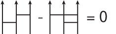 |
Clearly, these relations imply that the weight system satisfies the 4-term relation as well. As a result, the product and coproduct of section 2.2 are still well-defined. So we can give the vector space of chord diagrams for string links with components modulo the 2-term relations the structure of a bialgebra. We will denote this bialgebra (and the underlying vector space) by . There is a natural projection from to .
Similarly, we can look at the quotient space of by the 2-term relations
Since , the 2-term relations imply the 4-term relations, and the quotient space is a bialgebra with the product and coproduct induced from . is then a bialgebra homomorphism from to .
4.1 Chord diagrams for String Links modulo 2-term relations
Bar-Natan and Garoufalides [2] analyzed the space of chord diagrams for knots (equivalently, string links of one component) modulo the 2-term relations. They found that is generated (as a vector space) by ()-caravans of ”one-humped camels” (isolated chords which intersect no other chords) and ”two-humped camels” (pairs of chords which intersect each other, but no other chords). An example of such a caravan is shown in Figure 4.
 |
Our goal in this section is to find a similar ”normal form” for string link chord diagrams with more than one component; this will be useful in the remainder of the paper. We will prove the following theorem:
Theorem 2
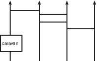
Any connected string link chord diagram is equivalent, modulo the 2-term relations, to a chord diagram with components numbered 1,…, n (possibly after renumbering) such that:
- •
Every chord either has both endpoints on component 1, or endpoints on components i and i+1 for some i.
- •
The chords with both endpoints on component 1 are arranged in a caravan. Moreover, all of their endpoints lie below the endpoints of any chords between components.
- •
There are at most 2 chords between components i and i+1, and if there are 2 they do not cross (so the endpoints of one chord lie above the endpoints of the other on both components).
- •
On component i, the endpoints of chords connecting component i to component i+1 lie below the endpoints of chords connecting component i to component i-1.
An example is shown in Figure 5.
 |
If a diagram is not connected, we simply put each connected component into normal form.
The proof proceeds in several steps. We will describe an algorithm to put any connected
chord diagram into the normal form described above via 2-term relations.
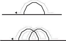
Step 1: We first deal with chords which have both endpoints on the same component. To begin with, any pair of intersecting chords which have all four endpoints on the same component can be slid to the bottom of the component, away from any other chords, to form a two-humped camel as in [2]. An isolated chord with both endpoints on the same component can also be slid down to the bottom, forming a one-humped camel. See Figure 6 for examples of these moves.
 |
We are left with chords with both endpoints on the same component which only intersect chords which lie between two different components. By sliding this chord over one of the chords it intersects, its endpoints are now on two different components, as shown in Figure 7.
 |
Step 2: Our next step is to put every chord connecting two different components on a different horizontal ”level”; in particular, we will remove intersections between chords between the same two components. Say that we have chords between components. Select a chord arbitrarily, which we will denote chord . Without loss of generality, assume connects components 1 and 2. We will move to the top level. As we move it up, if we come to a chord with an endpoint on components 1 or 2 which is above we move that endpoint below via a 2-term relation, as shown in Figure 8.
 |
Ultimately, the endpoints of will lie above the endpoints of any other chord. During
this process, some chords may have had both their endpoints moved to the same component -
remove or modify these chords as in Step 1 (notice that this only reduces the number of
chords between components from ). We are left with at most chords
connecting components, all below . So we can continue the process inductively, ending
with all chords between components horizontal, at different levels (and with a caravan at
the bottom of each component).
Step 3: Now we consider one component of the diagram, say component 1, and move all the chords with an endpoint on component 1 to a higher level than all the other chords in the diagram (leaving chords with both endpoints on the same component at the bottom). We will denote by an (i,j)-chord a chord with endpoints on components and . If a (1,)-chord lies directly below an ()-chord along component , we can use a 2-term relation to move the (1,)-chord above the other chord, in the process transforming it into a (1,)-chord, as in Figure 9.
 |
Since there are only a finite number of chords, we can successively move all chords with
one endpoint on component 1 above all other chords (while the other endpoint may move,
one will always remain on component 1).
Step 4: Let be the top chord at this point; without loss of generality,
is a (1,2)-chord. Let be the number of (1,)-chords, and . Now move down component 1, stripping other chords off of component
1 by 2-term relations, transforming them from (1,)-chords to (2,)-chords, reversing
the move from Step 2 shown in Figure 8. Continue this until encounters
another (1,2)-chord, . Now move back up as in Step 3 (see Figure 9);
when it is again at the top, it will be a (1,)-chord for some . Repeat the process
for , moving it up to just below , and with all the other (1,2)-chords. This
reduces to , though the chords may no longer be (1,2)-chords. We can
relabel the components so that is once again a (1,2)-chord and repeat the process.
Each repetition reduces , until we reach a point where (i.e. all
chords with an endpoint on component 1 are (1,2)-chords), and the (1,2)-chords lie above
all other chords in the diagram. Finally, we can reduce to 1 or 2 by noticing
that whenever , we can factor out a 2-humped camel and reduce by
2, as in Figure 10.
 |
Step 5: We can now repeat Steps 3 and 4 for component 2, and then for each component in turn. We are left with a diagram which is almost in normal form - the final step is to move all of the caravans to component 1. We can move a caravan from the th component to the th component by sliding it over a chord between the two components, as in Figure 11.
 |
Any other chords between the two components can be slid over the caravan in turn by 2-term relations, leaving the caravan below the chords connecting components and . Continuing in this way, the caravans can be moved to component 1, and finally pushed to to bottom of component 1 as in step 1. This completes the proof of Theorem 2.
4.2 Adjacency Matrices for Intersection Graphs
In this section we will define the adjacency matrix for an intersection graph, and show that its rank and determinant (over ) are regular graph weight systems.
Definition 7
Given a directed graph G with n vertices, , such that each vertex has a label , the adjacency matrix of G, or adj(G), is the matrix defined by:
These matrices can be viewed as bilinear forms over , but unlike the case for knots [13], they are not generally symmetric, so their classification is much more difficult (and still, to my knowledge, an open question). We are interested in the notion of congruence of such matrices. We are particularly interested in the adjacency matrices of semisymmetric graphs; which have the property (which we will also denote by semisymmetry) that if the th diagonal element is 0, then the th row and column are the same.
Definition 8
We say that two matrices A and B are congruent (denoted ) if there is an invertible matrix P such that .
One of our main results is that the congruence class of the adjacency matrix (over ) satisfies the 2-term relation, and so induces a regular graph weight system.
Theorem 3
For any graph G in E, .
Proof: Reordering the vertices of changes by a congruence; in
this case, is the result of doing a corresponding reordering of the rows of
the identity matrix. So we can assume that the first two rows and columns of
and correspond to the vertices and .
The matrices are identical except for the first row and column. Say that
has label and has label , so in has label
. An entry (where ) is equal to
(mod 2), and similarly for the first column.
if and only if , i.e. if
, so .
Finally, if , and 1 otherwise. We have
five cases.
Case 1: . In this case and
(due to the semisymmetry of the graph). So, mod 2,
.
Case 2: . In this case and
. So, mod 2, .
Case 3: . In this case, and ,
and . So, mod 2, .
Case 4: . In this case, and ,
and . So, mod 2, .
Case 5: all different. In this case
and . So, mod 2, .
We conclude that . Therefore and are congruent by a matrix , where is the elementary matrix constructed from the identity matrix by adding the second row to the first row. In other words, is the same as the identity, except for the 2 by 2 matrix in the upper left corner, which is .
Corollary 1
The congruence class of the adjacency matrix of the intersection graph is invariant under the 4-term relations.
Corollary 2
The determinant (mod 2) and rank (over ) of the adjacency matrix of the intersection graph are regular graph weight systems.
Proof: If is invertible over , the rank of is the same as the rank of . In addition, (mod 2), so the determinant is also a congruence invariant mod 2.
4.3 Relations to the Conway and Homfly polynomials
For knots, the Conway and Homfly weight systems can be interpreted via intersection graphs [13]. To what extent can we do the same for string links? In general, this is still an open problem, but we can offer a few initial results.
Let us recall the definitions of the Conway polynomial and weight system. The Conway polynomial of a link is a power series . It can be computed via the skein relation (where are as in Figure 12):
 |
We define the Conway polynomials of a string link as the Conway polynomial of the link formed by closing the string link in the natural way. The coefficient is a finite type invariant of type [1, 3], and therefore defines a weight system of degree . The collection of all these weight systems is called the Conway weight system, denoted . Consider a chord diagram , together with a chord . Let be the result of surgery on v, i.e. replacing by an band which preserves the orientation of the components, and then removing the interior of the band and the intervals where it is attached to , as shown in Figure 13
 |
(so may have multiple boundary circles). The skein relations for the Conway polynomial give rise to the following relations for :
It is easy to show [2] that this weight system satisfies the 2-term relations of section 4. Simply surger the two chords; the 2-term relation then says just that one band can be ”slid” over the other, which doesn’t change the topology of the diagram. Bar-Natan and Garoufalides also showed that the weight system for the Conway polynomial for knots is just the determinant of the adjacency matrix for the intersection graph, mod 2. The next theorem extends this result to string links with two components.
Theorem 4
For any chord diagram D on a string link with two components, (mod 2).
Proof: Since both of these weight systems satisfy the 2-term relations, it suffices to show that they agree on diagrams in normal form (see section 4.1). For string links with two components, normal form consists of a caravan on the first component, and 0, 1, or 2 parallel chords between the two components. Say that the caravan has 1-humped camels and 2-humped camels, and there are chords between the components (). Then . So (mod 2) and (mod 2). The product of the rank and determinant is 1 (mod 2) when and , and 0 otherwise.
On the other hand, if we surger all the chords of the diagram, and close the string link, we obtain an unlink with components when , and when , which means that only when and . So the two weight systems agree.
With more than two components, the situation is more complicated; in fact, the Conway weight system is not always determined by the adjacency matrix of the intersection graph. Figure 14 shows two chord diagrams and on 4 components which illustrate this.
 |
It is easy to see that these intersection graphs for these diagrams differ only in the labeling of the vertices, so:
However, surgering the chords in yields a string link whose closure has one component, and surgering the chords in yields a string link whose closure has 3 components. Therefore, , but .
However, we can at least give a sufficient condition for to be trivial which depends only on the adjacency matrix.
Proposition 1
Let D be a string link chord diagram of degree k on n components. If either of the following conditions holds, then C(D) = 0.
- •
.
- •
is even.
Proof: The first condition means that, in the normal form, there will be an isolated chord in the caravan, so will be trivial. The second condition comes from observing that every surgery of a chord in the number of components in the closure of by 1 (either adding or removing a component). Since we begin with components, the number of components after all the chords are surgered is congruent to modulo 2. So can be non-trivial only if mod 2. Hence, if is even, then .
Now we will consider the (framed) Homfly weight system for string links. The Homfly invariant is the Laurent polynomial defined by the following skein relations [11] ( is the result of adding a positive kink to the link ):
If we make the substitutions and , and expand the resulting power series, we transform the Homfly polynomial into a power series in , whose coefficients are finite type invariants (of regular isotopy). These invariants give rise to regular weight systems which we can collect together as the Homfly regular weight system . The skein relations above give rise to the following relations for , by looking at the first terms of the power series (as before, is the result of surgering the chord in ):
So if is an unlink of components, . Since the first of these relations is almost the same as for the Conway weight system , the same argument shows that satisfies the 2-term relations. We can now consider string link diagrams with two components (as with the Conway weight system, the Homfly weight system is not necessarily determined by the adjacency matrix of the intersection graph for chord diagrams on more than two components).
Theorem 5
For any chord diagram D of degree k on a string link with 2 components, let . If r is odd, then ; if r is even, then .
Proof: As with Theorem 4, it suffices to show that the weight systems agree on diagrams in normal form. Let be the diagram with one-humped camels and two-humped camels on component 1, and chords between the two components () (so the degree of is ). As before, , so the rank is . is even when and odd when .
On the other hand, if we surger all the chords (each time multiplying by
), the resulting link has components when (and is
even), and components when (and is odd). So when is
even, , and when is odd, .
Remark: If we let and , then . According to
Theorem 5, if is a string link chord diagram with two components, we will
have in this case unless is odd (in which case ).
But this is exactly the case when (since the matrix has full rank) and
mod 2, so . So the formulas for the Conway and Homfly
weight systems agree in this case.
5 Further Questions and Problems
There are several obvious questions and directions for further research.
Question 1
To what extent are the Conway and Homfly weight systems for string links with more than two components determined by the intersection graph?
Figure 14 gives an example of chord diagrams on 4 components where the adjacency matrix of the intersection graph is insufficient to determine the Conway and Homfly weight systems. However, this example seems to depend strongly on there being 4 components - it is not clear how to find connected examples with, say, 5 components where the adjacency matrix is insufficient. And certainly the adjacency matrix (as shown by the example in Figure 14 does not contain all the information of the intersection graph - in particular, the information contained in the vertex labels. This leads to our next question:
Question 2
Can we find invariants of intersection graphs other than the adjacency matrix which give rise to weight systems?
Question 3
Can we find other invariants of string links whose weight systems can be computed via intersection graphs?
The author has looked at Milnor’s homotopy invariants for string links [16], but there are many others.
Question 4
To what extent does the intersection graph determine the chord diagram?
This question is still open for knots, as well, though some progress has been made [6, 12]. Some work has been done by the author [14] for the case when the intersection graph is a tree, but this is only a bare beginning.
Question 5
Can we generalize these constructions from string links to links?
We should be able to define intersection graphs for links as a quotient space of the intersection graphs for string links. It is yet to be seen whether this is useful.
References
- [1] Bar-Natan, D.: On the Vassiliev Knot Invariants, Topology 34, No. 2, pp. 423-472, 1995
- [2] Bar-Natan, D. and Garoufalidis, S.: On the Melvin-Morton-Rozansky Conjecture, Invent. Math. 125, pp. 103-133, 1996
- [3] Birman, J. and Lin, X.S.: Knot polynomials and Vassiliev’s Invariants, Invent. Math. 111, pp. 225-270, 1993
- [4] Bouchet, A.: Circle Graph Obstructions, Journal of Combinatorial Theory, Series B, 60, pp. 107-144, 1994
- [5] Chmutov, S.V. and Duzhin, S.V.: The Kontsevich Integral, Acta Applicandae Math., Vol. 66, pp. 155-190, 2001
- [6] Chmutov, S.V., Duzhin, S.V. and Lando, S.K.: Vassiliev Knot Invariants I, II, III, Advances in Soviet Mathematics 21, pp. 117-145, 1994
- [7] Habegger, N. and Lin, X.S.: The Classification of Links up to Link-Homotopy, J. of the Amer. Math. Soc., Vol. 3, No. 2, 1990, pp. 389-419
- [8] Kontsevich, M.: Vassiliev’s knot invariants, Advances in Soviet Mathematics, Vol. 16, Part 2, pp. 137-150, 1993
- [9] Lando, S.: On a Hopf algebra in graph theory, Journal of Combinatorial Theory, Series B, v.80, p. 104-121, 2000
- [10] Le, Thang: unpublished, 1996
- [11] Lickorish, W.B.: An Introduction to Knot Theory, GTM vol. 175, Springer, New York, 1997
- [12] Mellor, B.: The Intersection Graph Conjecture for Loop Diagrams, Journal of Knot Theory and its Ramifications, Vol. 9, No. 2, 2000. Also see arXiv:math.GT/9807033
- [13] Mellor, B.: A few weight systems arising from intersection graphs, Michigan Math. J., Vol. 51, No. 3, pp. 509-536, 2003. Also see arXiv:math.GT/0004080
- [14] Mellor, B.: Tree diagrams for string links, preprint, May 2004, arXiv:math.GT/0405537
- [15] Mellor, B.: Tree diagrams for string links II: Determining Chord Diagrams, preprint, August 2004, arXiv:math.GT/0408286
- [16] Mellor, B.: Weight systems for Milnor invariants, in preparation
- [17] Meng, G.: Bracket models for weight systems and the universal Vassiliev invariants, Topology and its Applications 76, pp. 47-60, 1997
- [18] Morton, H.R. and Cromwell, P.R.: Distinguishing Mutants by Knot Polynomials, Journal of Knot Theory and its Ramifications 5, No. 2, pp. 225-236, 1996
- [19] Milnor, J. and Husemoller, D.: Symmetric Bilinear Forms, Springer-Verlag, New York, 1973
- [20] Stanford, T.: Finite-Type Invariants of Knots, Links, and Graphs, Topology 35, No. 4, pp. 1027-1050, 1996
- [21] Vassiliev, V.A.: Cohomology of knot spaces, in Theory of Singularities and Its Applications (ed. V.I. Arnold), Advances in Soviet Mathematics, Vol. 1, pp. 23-69, 1990