A New Way to Compute the Thurston-Bennequin Number
Abstract.
We establish a relation between several easy-to-calculate numerical invariants of generic knots in , and use it to give a new method of computing the Thurston-Bennequin number of Legendrian knots in the tight contact .
1. introduction
A contact structure on is an oriented positively nowhere integrable tangent plane distribution, i.e., is oriented as a -plane distribution, and there is a -form on such that , , and . Such a -form is called a contact form for . A knot in is said to be Legendrian in if it is tangent to everywhere. is said to be overtwisted if there is an embedded disk in such that is Legendrian, but is transversal to along . A contact structure that is not overtwisted is called tight. In [4, 5], Y. Eliashberg proved that any tight contact structure on is isotopic to the standard contact strcture given by the contact form , where are the standard Cartesian coordinates of .
There are two ”classical” invariants of Legendrian knots in a contact , the Thurston-Bennequin number and the Maslov index . We call the framing of a Legendrian knot given by the contact planes its contact framing. The Thurston-Bennequin number is defined to be the index of the contact framing of a Legendrian knot relative to its Seifert framing. And the Maslov index is the obstruction of extending the unit tangent vector of a Legendrian knot to a non-vanishing section of the contact plane bundle over its Seifert surface. See, e.g., [1, 3, 7] for more about these invariants. In , there are two methods to calculate these invariants. First, one can project a Legendrian knot onto the -plane, and get an immersed knot diagram, which we call the Legendrian projection. Then the Thurston-Bennequin number is the writhe of the diagram, and the Maslov index is the degree of the Gauss map of the diagram. Second, one can project onto the -plane, and get a knot diagram with cusps but no vertical tangents, which we call the front projection. Then the Thurston-Bennequin number is the writhe of the diagram minus half of the number of cusps, and the Maslov index is half of the number of cusps tranversing downward minus half of the number of cusps tranversing upward. See Figure 1 for an example.
In this paper, we consider the contact structure given by , where are the standard cylindrical coordinates of . It is isotopic to the standard contact structure (see, e.g., [6]). We first define some easy to calculate knot invaraints in , and then use these to compute and for Legendrian knots in disjoint from the -axis. (This is the generic situation since any Legendrian knot can be make disjoint from the -axis by small Legendrian isotopy.)
2. Definitions of Invariants
The -dimensional hyperbolic space is defined to be the upper half plane equipped with the metric . is the unit tangent bundle of , i.e., the -bundle over formed by tangent vectors of length . There is a natural orientation preserving diffeomorphism given by
| (1) |
Let be with the -axis removed. Then there is a natural orientation preserving diffeomorphism given by
| (2) |
In the rest of this paper, we will always identify these three manifolds by the diffeomorphisms and .
An embedding of into is a called knot. The standard orientation of induces an orientation on every knot. Unless otherwise specified, all knots in this paper are oriented this way. Since , and the homology class of a -fiber is a generator of , we have that, for any knot in , there is a unique integer satisfying .
Definition 2.1.
is called the homology of the knot .
A knot in is said to be generic if it is nowhere tangent to the -fibers. Two generic knots are said to be generically isotopic if they are isotopic through generic knots. Let be the projection onto the first factor. For any generic knot , is an immersed curve in .
For an immersed curve in , the canonical lifting of to is defined to be , where is the arc length element of .
Definition 2.2.
For a generic knot in , define the rotation number of to be , where is the canonical lifting of .
Let be the tangent vector field on formed by the unit tangent vectors of the -fibers. For any generic knot , gives a framing. We call this framing the canonical framing for . Also, as a knot in , has a Seifert surface in . This surface gives a framing, called the Seifert framing for . Note that the Seifert framing is well defined, i.e., it is independent of the choice of the Seifert surface.
Definition 2.3.
The self linking number of a generic knot is defined to be the index of the canonical framing with respect to the Seifert framing.
Equivalently, can be defined to be the intersection number of and , where is the knot given by pushing slightly in the direction of , and is a Seifert surface of in .

Let be a generic knot, and a transversal double point of . Let be the two pre-images of . The signs here are assigned in such a way that is an oriented basis for . Note that and are on the same -fiber. Denote this fiber by . Let be the part of starting from and ending in , and the part of starting from and ending in . Cutting open at and , we get two embedded open oriented curves and in , where is the one starting from ending in , and is the one starting from ending in . Let be the knot formed by , and the knot formed by . Define the weight of to be .
We can always isotope a generic knot slightly (hence, generically) so that the only singularities of the projection on of the perturbed generic knot are transversal double points.
Definition 2.4.
Let be a generic knot, and a generic knot generically isotopic to such that the only singularities of are transversal double points. The winding number of is defined to be sum of the weights of all the transversal double points of .
We need demonstrate that the winding number is well defined and is invariant under generic isotopy. To do this, we only need show that, if two generic knots are generically isotopic, and the only singularities of their projections on are transversal double points, then the sums of the weights of all the transversal double points of the two knots are equal. The proof of this fact is straightforward. Note that, if two such knots are generically isotopic, we can change one of them to the other by a series of local moves corresponding to second type and third type Reidemeister moves of its projection. There is a natural correspondence between the transversal double points of two projections differed by a third type Reidemeister move. One easily checks that the weights of corresponding double points are the same. It is also easy to check that, in a second type Reidemeister move, the sum of the weights of the two transversal double points to be created or to be cancelled is always . Thus, the winding number is indeed well defined and invariant under generic isotopy.
3. Relating , , and
Theorem 3.1.
Let be a generic knot in . Then
To prove Theorem 3.1, we need use the universal first order invariant defined by Chernov in [2]. We now briefly introduce the definition of this invariant in our settings. For more details, see [2].
Choose a base point in , and let be the group modulo the actions of via conjugation on both summands, and the action of by permuting the two summands. There is a natural isomorphism from to by mapping the fiber thought to . So we can identify with the set of unordered pairs of integers. Denote such a pair by . Then, . We denote by the free -module generated by .
Now, let be a generic knot such that the only singularities of its projection on are transversal double points. We equip with the canonical framing. Then the invariant of the framed knot is defined by
where the sum is taken over all transversal double points of . The invariant assigns an element of to every framed knot in , and is invariant under isotopy of framed knots.
Now let be the -linear mapping such that for . Then a simple calculation reveals the following.
Proposition 3.2.
Let be a generic knot in equipped with the canonical framing. Then .
With Proposition 3.2 in hand, it’s clear that Theorem 3.1 is a direct consequence of Proposition 3.3 below.
Proposition 3.3.
Let be a generic knot in equipped with the canonical framing. Then .
Proof.
Note that is indeed an invariant of framed knots, i.e., if two generic knots equipped with the canonical framing are isotopic as framed knots, then the value of their -invariants are the equal. So, is also an invariant of framed knots. Let be a framed singular knot in , whose only singularity is a transversal self-intersection of two strands. Up to isotopy, there are two ways to resolve this singularity. Let the two strands intersecting at the singularity be and . As in [2], we denote by the resolution of such that the tangent vector of , the tangent vector of , and the vector from to form a position basis for , and denote by the other resolution of . Then, , and, according to Theorem 1.2.5(2) of [2], . This shows that, if two framed knots and are differed by a crossing of two transversal strands, then . Since any homotopy between two framed knots, after a possible slight perturbation, can be decomposed into a sequence of isotopies and crossings of transversal strands, is indeed a homotopic invariant of framed knots. Note that any framed knot of homology is homotopic to one of the two knots depicted in Figure 3 equipped with canonical framing. A straightforward calculation shows that for both of these knots. Thus, for all framed knots in . ∎
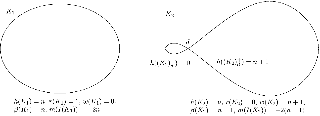
4. Computing and
Since the standard hyperbolic metric on has curvature , its Levi-Citita connection form is a positive contact form on . Under the identification and , the corresponding contact structures on and are defined by , and , respectively. Note that the latter is the restriction of on .
Clearly, every Legendrian knot in is generic. So, every invariant in this paper induces an invariant of Legendrian knots in . The Thurston-Bennequin number and the Maslov index in restrict to invariants of Legendrian knots in . Their relations with the invariants defined in Section 2 are described in Theorem 4.1.
Theorem 4.1.
Let be a Legendrian knot in . Then,
- (1)
,
- (2)
.
Proof.
Note that is transverse to the contact plane field. So, by definition, . The rest of part (1) is just Theorem 3.1.
Let be the natural projection. Then equals the degree of the Gauss map of . Define the map by . Then and are homotopic through immersed curves in . So their Gauss maps have the same degree.
Let be the standard rectangular coordinates of , i.e., . Then the map is given by
Let be a regular parameter of . We calculate the degree of the Gauss map of . First, we have
Then we substitute by , and apply the relation . This gives
But
and
This proves part (2). ∎
References
- [1] D. Bennequin, Entrelacements et équations de Pfaff, Astérisque, 107-108 (1983), 87–161.
- [2] V. Chernov, The universal order one invariant of framed knots in most -bundles over orientable surfaces, Algebr. Geom. Topol 3 (2003), 89–101 (electronic).
- [3] Y. Eliashberg, Legendrian and transversal knots in tight contact -manifolds, Topological methods in modern mathematics (Stony Brook, NY, 1991), 171–193, Publish or Perish, Houston, TX, 1993.
- [4] Y. Eliashberg, Contact -manifolds twenty years since J. Martinet’s work, Ann. Inst. Fourier (Grenoble) 42 (1992), no. 1-2, 165-192.
- [5] Y. Eliashberg, Classification of contact structures on , Internat. Math. Res. Notices 1993, no. 3, 87-91.
- [6] J. Etnyre, Introductory Lectures on Contact Geometry, Proc. Sympos. Pure Math. 71 (2003), 81-107.
- [7] D. Fuchs, S. Tabachnikov, Invariants of Legendrian and transverse knots in the standard contact space, Topology 36 (1997), no. 5, 1025–1053.