Polynomial invariants of links in the projective space

The Homfly and Kauffman polynomials of links in $\mathbb{R}^{3}$ are defined by skein relations.

For Homfly polynomial, the skein relations are:

(HI) $x^{-1}\vbox{\hbox{\psfig{file}}}-x\vbox{\hbox{\psfig{file}}}=(s-s^{-1})\vbox{\hbox{\psfig{file}}}$

(HII) $\vbox{\hbox{\psfig{file}}}=(xv^{-1})\vbox{\hbox{\psfig{file}}}$

In these relations, links are presented by their fragments which contain differences from other links under consideration. Moreover, the Homfly polynomial of a link is written simply as the link itself.

The relations (HI) and (HII) together with the assumption that the polynomial is equal to 1 on the unknot determine the polynomial for any framed oriented link in $\mathbb{R}^{3}$ and this polynomial is invariant under isotopy of such links.

Similarly, for Kauffman polynomial the skein relations are:

(KI) $\vbox{\hbox{\psfig{file}}}+\vbox{\hbox{\psfig{file}}}=z\left(\vbox{\hbox{\psfig{file}}}+\vbox{\hbox{\psfig{file}}}\right)$

(KII) $\vbox{\hbox{\psfig{file}}}=a\vbox{\hbox{\psfig{file}}}$

The relations (KI) and (KII) together with the assumption that the polynomial is equal to $1$ on the unknot determine the polynomial for any framed unoriented link in $\mathbb{R}^{3}$ and this polynomial is invariant under isotopy of such links.

Homfly and Kauffman polynomials can be extended to links in any oriented 3-manifold through the notion of skein modules [3].

For an oriented 3-manifold $M$, the Homflypt skein module of $M$ is the module over the ring $\mathbb{Z}[x^{\pm 1},s^{\pm 1},(s-s^{-1})^{-1},v^{\pm 1}]$, generated by isotopy classes of framed oriented links in $M$, with relations (HI) and (HII). The Kauffman skein module of $M$ is the module over $\mathbb{Z}[a^{\pm 1},z^{\pm 1}]$, generated by isotopy classes of framed unoriented links in $M$, with relations (KI) and (KII).

Note that if $M$ is $\mathbb{R}^{3}$, the Homflypt and Kauffman skein modules are free cyclic modules generated by the unknot. The Homfly polynomial (resp. Kauffman polynomial) of a framed oriented link (resp. framed unoriented link) is obtained by expressing the link with the unknot: in the corresponding skein module the link equals to the corresponding polynomial multiplied with the unknot.

For $n>0$, the standard oriented unlink in $\mathbb{R}P^{3}$ with $n$ noncontractible components, denoted by $L_{n}$, is the link presented in Figure 1 ($\mathbb{R}P^{3}$ is represented as a ball $D^{3}$ with antipodal points of the bounding sphere identified). $L_{0}$ is the unknot . The framing for each $L_{n}$ (a line framing) is the blackboard one.

This theorem is a consequence of the following:

The standard unoriented unlink in $\mathbb{R}P^{3}$ with $n$ noncontractible components, again denoted by $L_{n}$, is the link presented in Figure 1 with the orientations being disregarded. $L_{0}$ is the unknot . The framing for each $L_{n}$ is the blackboard one.

This theorem is a consequence of the following:

The choices for $H(L_{0})$ and $K(L_{0})$ are convenient for constructions of $H$ and $K$. These choices are consistent with $H$ and $K$ being equal to 1 for the empty link. Also, with these choices, $H$ and $K$ are multiplicative under disjoint union. Note that in the case of projective links, the disjoint union is well defined on couples consisting of one affine link and one projective link.

A diagram of a link in $\mathbb{R}P^{3}$ is a disk with a collection of immersed arcs. An arc is a compact connected 1-manifold with or without boundary. The endpoints of arcs with boundary are on the boundary of the disk, divided into pairs of antipodal points and, with this restriction, the arcs are immersed generically. Each double point of the immersions or crossing of the diagram is endowed with information of over- and undercrossing.

A net is the projective plane $\mathbb{R}P^{2}$ together with a distinguished (projective) line, called the line at infinity, and a collection of generically immersed circles endowed with information of over- and undercrossing for each double point. We can map any diagram $D$ of a link to its net, obtained from $D$ by identifying the antipodal points of the boundary circle of $D$, with the line at infinity being the image of this boundary circle.

If $D$ is a diagram of a link $L$ and $L_{b}$ is a connected component of $L$, then the projection of $L$ onto $D$ maps $L_{b}$ onto a collection of arcs. Denote this collection by $b$. We will call $b$ a component of $D$ (though it may consists of several arcs). As $H_{1}(\mathbb{R}P^{3})=\mathbb{Z}_{2}$ there are two types of connected components in a link: 0-homologous and non 0-homologous. The corresponding components of a diagram of the link, are said to be 0-homologous (their images in the net are contractible) and 1-homologous (their images in the net are not contractible).

If $D$ is a diagram of an oriented link $L$, $D$ gets naturally oriented: each of its arcs is oriented. If $b$ is a component of $D$ coming from a component $L_{b}$ of $L$, then the orientation of $L$ gives rise to a cyclic ordering of arcs of $b$ (when one travels on $L_{b}$ according to the orientation, one meets the arcs of $b$ in this order under the projection of $L$ onto $D$).

Let $D$ be a diagram of an oriented link and $b$ a component of $D$. Let $P$ and $Q$ be two points in the interior of some arcs of $b$. Then the arc distance from $P$ to $Q$ is defined to be the number of times the line at infinity is crossed in the net of $D$, if one travels from the image of $P$ to the image of $Q$ in the net, according to the orientation of the image of $b$ in the net.

Suppose that $X$ is a crossing of $D$ such that at least one of its branches is in $b$. Then the first pass of $X$ from $P$ is, by definition, the branch of $X$ whose image in the net of $D$ is passed first, if one travels from the image of $P$ in the net, according to the orientation of the image of $b$ in the net.

Suppose that $P$ and $Q$ are distinct. $D$ is said to be descending from $P$ to $Q$ if, for every crossing $X$ encountered when traveling from $P$ to $Q$ in the net according to the orientation, the first pass of $X$ from $P$ is an overpass (resp. underpass), if the arc distance from $P$ to this first pass is even (resp. odd). One says that $D$ is descending from $P$ to $P$ if it is descending from $P$ to $Q$, where $Q$ is a point on the same arc as $P$ and such that one can travel on this arc from $Q$ to $P$ according to the orientation without passing any crossing (i.e. $Q$ is just before $P$).

If $D$ is descending from $P$ to $Q$, then, traveling on the net from $P$ to $Q$, the encountered arcs are alternatively descending and ascending in the usual meaning for links in $\mathbb{R}^{3}$.

There is a function $H$ defined on the set of diagrams with at most $(n-1)$ crossings, taking values in $\mathbb{Z}[x^{\pm 1},s^{\pm 1},(s-s^{-1})^{-1},v^{\pm 1},z]$ such that:

1. (1)

   $H$ is invariant under those Reidemeister moves that do not increase the number of crossings beyond $n-1$.

2. (2)

   $H$ satisfies relations (HI) and (HII).

3. (3)

   If $D$ is the standard diagram of standard oriented unlink $L_{m}$, $m>0$, with at most $(n-1)$ crossings (i.e. $m(m-1)/2\leq n-1$), then $H(D)=z^{m}$. Also, $H(\vbox{\hbox{\psfig{file}}})=\mu$.

As the definition of $H$ uses induction on the number of crossings, $H$ is first defined for diagrams with 0 crossings.

Let $D$ be a diagram with 0 crossings. Let $p$ be the number of its 0-homologous components and $m$ the number of its 1-homologous components ($m$ is 0 or 1). Then, by definition:

$(H_{1}):H(D)=\mu^{p}z^{m}$

For convenience $H$ of the empty link is, by definition, equal to 1 (which agrees with $(H_{1})$). Note that $H$ satisfies IH(0).

We assume that the inductive hypothesis IH($n-1$) holds true.

The construction of $H$ for diagrams with $n$ crossings is divided into several cases treated in the subsequent subsections. In each case a diagram $D$ with $n$ crossings is endowed with some extra structure (a basepoint or a couple of basepoints). $D$ together with this structure is denoted by $\dot{D}$. A diagram $\alpha(\dot{D})$ is then defined: it is a diagram obtained from $\dot{D}$ by a series of crossing changes.

The diagram $\alpha(\dot{D})$ has the following property: if $X$ is one of the crossings of $\dot{D}$ that have to be switched to obtain $\alpha(\dot{D})$, and $\dot{D}^{\prime}$ is the diagram obtained from $\dot{D}$ by switching $X$, then $\alpha(\dot{D})=\alpha(\dot{D}^{\prime})$.

In the following subsections $H$ is defined on $\alpha(\dot{D})$ for each case (see $(H_{3})$ to $(H_{6})$).

Suppose that $H$ is already defined on all $\alpha(\dot{D})$. For a based diagram $\dot{D}$, denote by $S(\dot{D})$ the set of crossings of $\dot{D}$ where $\dot{D}$ and $\alpha(\dot{D})$ differ. Let $k$ be the number of elements in $S(\dot{D})$ and $\omega$ a (linear) ordering of $S(\dot{D})$. Denote by $S(\dot{D},\omega)$ the set $S(\dot{D})$ equipped with ordering $\omega$.

We define $H(\dot{D},\omega)$ by induction on $k$. The definition depends on $\omega$. If $k=0$ then $H$ is already defined. Otherwise let $\dot{D}^{\prime}$ be the based diagram obtained from $\dot{D}$ by switching the first crossing in $S(\dot{D},\omega)$ and $D^{\prime\prime}$ be the diagram obtained by smoothing the same crossing. Let $\omega^{\prime}$ be an ordering of all crossings of $S(\dot{D^{\prime}})$ induced by $\omega$. Note that there are $k-1$ elements in $S(\dot{D^{\prime}})$. $H(\dot{D}^{\prime},\omega^{\prime})$ is defined by induction on $k$ and $H(D^{\prime\prime})$ is defined by IH($n-1$). Now $H(\dot{D},\omega)$ is defined using the relation (HI) on the first crossing in $S(\dot{D},\omega)$ with the help of $H(\dot{D}^{\prime},\omega^{\prime})$ and $H(D^{\prime\prime})$. Namely, if $\epsilon$ is the sign of this first crossing, then, by definition:

$(H_{2}):H(\dot{D},\omega)=x^{2\epsilon}H(\dot{D}^{\prime},\omega^{\prime})+\epsilon x^{\epsilon}(s-s^{-1})H(D^{\prime\prime})$

A diagram is said to be simple, if it has at least one 1-homologous component and any of its crossings involves two different 1-homologous components. Thus, a simple diagram has no crossings involving 0-homologous components and no self-crossings of 1-homologous components.

A based simple diagram $\dot{D}$ (the dot indicates that the diagram is based) is a simple diagram $D$ equipped with a couple of basepoints. The basepoints are antipodal points that lie on the boundary circle of the diagram and that are endpoints of some arc(s) of a 1-homologous component. They are indicated by black dots.

The antipodal basepoints are also called primary basepoints. They give rise to an ordering of 1-homologous components and a couple of antipodal basepoints, called secondary, on each of them (except the component that has the primary basepoints), in the following way: if one travels on the boundary of the disk from the primary basepoints, one encounters, for each 1-homologous component, a couple of endpoints belonging to it. For each such component, the couple encountered for the first time is by definition the couple of secondary basepoints. It is indicated by a couple of white dots. The 1-homologous components are ordered starting with the component with the primary basepoints, then the component whose secondary basepoints are encountered first and so on, until the component whose secondary basepoints are encountered last. An example of based simple diagram with a couple of primary basepoints and two couples of secondary basepoints is shown in Figure 2.

Denote by $\dot{D}_{k,l}$ the based diagram shown in Figure 3. It is called standard based diagram. A based simple diagram $\dot{D}$ is said to be almost standard, provided that it can be transformed into some $\dot{D}_{k,l}$ by removing all 0-homologous components and performing a (possibly empty) series of crossing changes.

For any almost standard diagram $\dot{D}$, let $\alpha(\dot{D})$ be the based diagram obtained from $\dot{D}$ by switching all the crossings with sign $-1$. Thus $\alpha(\dot{D})$ has +1 sign at each crossing.

Let $p$ be the number of 0-homologous components of $\dot{D}$ and $m$ the number of its 1-homologous components. Then, by definition:

$(H_{3}):H(\alpha(\dot{D}))=\mu^{p}z^{m}$

An oriented arc with two endpoints has an initial endpoint and a final one. Notice that in an oriented diagram, any couple of antipodal endpoints consists of one initial and one final endpoint.

Let $\dot{D}$ be a simple based diagram. Consider the endpoint in the couple of primary basepoints of $\dot{D}$ which is initial. Now travel on the boundary of the disk in the counterclockwise direction from this endpoint and consider each encountered endpoint in the couples of secondary basepoints. It can be either initial or final. One says that a component is good if this encountered endpoint is initial and bad if it is final. The component to which the primary basepoint belongs is always a good component. Note that $\dot{D}_{k,l}$ has $k$ good components followed by $l$ bad ones.

One says that an arc $b$ follows an arc $a$, if the endpoint of $b$ that is initial, is antipodal to an endpoint of $a$ (which has to be final). An arc is above (resp. below) a component if, at each crossing involving the arc and the component, the upper (resp. lower) branch belongs to the arc.

A simple based diagram $\dot{D}$ is said to be descending if, for any 1-homologous component $b$, the arc of $b$ that contains the basepoint of $b$ which is initial, is above components coming after $b$ according to the order given by the primary basepoints; the arc that follows it is below the same components; and alternating in this way, for all the arcs of $b$.

For any simple based diagram $\dot{D}$, that is not almost standard, let $\alpha(\dot{D})$ be the based diagram obtained from $\dot{D}$ by crossing changes that make it descending.

Consider the crossings of $\dot{D}_{k,l}$ with sign $-1$. Each such crossing is a crossing between $i$-th good and $j$-th bad component so it may be indexed by $(i,j)$. Let $\omega_{k,l}$ be the lexicographical order of the set of all crossings with sign $-1$, indexed in this way.

Let $p$ be the number of 0-homologous components of $\dot{D}$, $k$ the number of good components and $l$ the number of bad components. Then, by definition:

$(H_{4}):H(\alpha(\dot{D}))=\mu^{p}H(\dot{D}_{k,l},\omega_{k,l})$

Note that in the case of an almost standard diagram $\dot{D}$, $\alpha(\dot{D})$ is not descending unless there are only good components in $\dot{D}$. In what follows, it is more convenient to have $\dot{D}_{k,l}$ descending rather than $\alpha(\dot{D}_{k,l})$.

A notion of based diagram, different from the one used for simple diagrams, is needed in order to construct $H$ for non simple diagrams. Let $D$ be a non simple diagram. A basepoint can be of two different kinds:

1. (1)

   A point on a 0-homologous component in the interior of some arc and distinct from any crossing if this component is involved in some crossings (see Figure 4(a)).

2. (2)

   A self-crossing of a 1-homologous component (see Figure 4(b)).

As before, a diagram $D$ equipped with a basepoint is denoted by $\dot{D}$.

First, we consider $\dot{D}$ for which the basepoint is on a 0-homologous component. $\dot{D}$ is said to be descending, if it is descending from the basepoint to the basepoint. If $\dot{D}$ has a basepoint on a 0-homologous component, the diagram $\alpha(\dot{D})$ is the based diagram obtained from $\dot{D}$ by the crossing changes that are necessary to make it descending.

Let $D^{\prime}$ be the diagram obtained from $\dot{D}$ by removing the component with the basepoint. Let $w$ be the sum of all signs at all self-crossings of the component with the basepoint in $\alpha(\dot{D})$. Then, by definition:

$(H_{5}):H(\alpha(\dot{D}))=\mu(xv^{-1})^{w}H(D^{\prime})$

Finally, we define $H$ in the case when the basepoint of $\dot{D}$ is a self-crossing of a 1-homologous component.

Let $X$ be a self-crossing of a 1-homologous component, say $b$. A smoothing at $X$ according to any orientation of $b$ gives rise to two components: one 0-homologous, the other 1-homologous. The dashed part determined by $X$ is the part of $D$ corresponding to the 0-homologous component.

Let $P$ and $Q$ be two points on $b$ such that, with respect to the orientation, $P$ is just before $X$, $Q$ is just after $X$ and $P$ and $Q$ are not in the dashed part determined by $X$ (see Figure 4(b)). Then $\dot{D}$ is said to be descending, if it is descending from $P$ to $Q$ (i.e. the dashed part is descending). If $\dot{D}$ has a basepoint which is a self-crossing of a 1-homologous component, the diagram $\alpha(\dot{D})$ is the based diagram obtained from $\dot{D}$ by the crossing changes which are necessary to make it descending.

Let $D^{\prime}$ be the diagram obtained from $\dot{D}$ by removing the dashed part determined by the basepoint. Let $w$ be the sum of signs at all self-crossings of the dashed part determined by the basepoint in $\alpha(\dot{D})$, including the basepoint (which is a self-crossing). Then, by definition:

$(H_{6}):H(\alpha(\dot{D}))=(xv^{-1})^{w}H(D^{\prime})$

The following lemma is a consequence of relation (HI):

In this section, it is shown that $H$ does not change under some Reidemeister moves that do not involve diagrams with more than $n$ crossings. It will be proven in latter sections that $H$ does not change under other moves. These other moves or bad moves are presented in Figure 6. They involve basepoint or basepoints.

The bad moves $\Omega_{4}^{\prime}$, $\Omega_{5}^{\prime}$ and $\Omega_{5}^{\prime\prime}$ involve simple based diagrams. The bad $\Omega_{4}^{\prime}$ move is the move in which, for some component, the secondary basepoints are changed. The bad $\Omega_{5}^{\prime}$ move involves two couples of secondary basepoints and the bad $\Omega_{5}^{\prime\prime}$ move involves the primary and some secondary basepoints.

All other moves are good moves. For these moves the proof that $H$ is unchanged is similar to the case of Homfly for links in $\mathbb{R}^{3}$ (see [6]).

Using relation (HI) and induction IH($n-1$) one gets easily the following:

In this section it is shown that $H$ does not depend on the choice of antipodal basepoints for simple diagrams.

We say that an arc in a diagram $D$ separates a couple $P$, $Q$ of antipodal points lying on the boundary $S$ of the disk of $D$, if the endpoints of this arc are in different connected components of $S-(P\cup Q)$. Otherwise, we say that the arc does not separate the couple.

The following lemma is a reformulation of Lemma 1 of [7]:

A subarc is a compact connected submanifold of an arc.

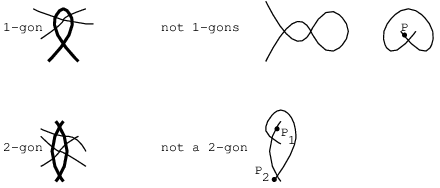
Let $a$ be a subarc going from a crossing to itself, such that it has no other self-crossings. Let $P$ be a point on the arc of which $a$ is a subarc, just outside $a$. Then $a$ is called a 1-gon if, in the net, it does not separate $P$ and the line at infinity.

Let ($a_{1}$, $a_{2}$) be a couple of subarcs both going from one crossing to another, having no extra crossings between them, and none of them having self-crossings. Let $P_{1}$ be a point on an arc of which $a_{1}$ or $a_{2}$ is a subarc, just outside $a_{1}$ and $a_{2}$, and close to the first crossing between $a_{1}$ and $a_{2}$. Let $P_{2}$ be a point with the same properties as $P_{1}$ except that it is close to the second crossing between $a_{1}$ and $a_{2}$. Then ($a_{1}$, $a_{2}$) is called a 2-gon if, in the net, it does not separate $P_{1}$ and the line at infinity and it does not separate $P_{2}$ and the line at infinity.

References

- [1] J. V. Drobotukhina, An analogue of the Jones polynomial for links in and a generalization of the Kauffman-Murasugi theorem, Algebra i analiz 2 (1990), no. 3, 171-191; English transl., Leningrad Math. J. 2 (1991), no. 3, 613-630.
- [2] P. Freyd, D. Yetter, J. Hoste, W.B.R. Lickorish, K. Millett, A. Ocneanu, A new polynomial invariant of knots and links, Bulletin of the American Mathematical Society, 12 (2) (1985) 239-246.
- [3] J. Hoste, J. Przytycki, A survey of skein modules of 3-manifolds, Knots 90 (Osaka, 1990), 363-379, de Gruyter, Berlin, 1992.
- [4] V. F. R. Jones, A polynomial invariant for knots via von Neumann algebras, Bulletin of the American Mathematical Society, 12 (1985), 103-111.
- [5] L. H. Kauffman, An invariant of regular isotopy, Transactions of the American Mathematical Society 318 (1990), no. 2.
- [6] W. B. R. Lickorish, K. C. Millett, A polynomial invariant of oriented links, Topology 26 (1987), no. 1, 107-141.
- [7] M. Mroczkowski, Diagrammatic unknotting of knots and links in the projective space, Journal of Knot Theory and Ramifications 12 (2003), no. 5, 637-651.