Horn’s Problem, Vinnikov Curves and the Hive Cone
Abstract
A Vinnikov curve is a projective plane curve which can be written in the form for , and positive definite Hermitian matrices. Given three -tuples of positive real numbers, , and , there exist , and with singular values , and and if and only if there is a Vinnikov curve passing through the points , and . Knutson and Tao proved that another equivalent condition for such , and to exist is that there is a hive (defined within) whose boundary is . The logarithms of the coefficients of approximately form such a hive; this leads to a new proof of Knutson and Tao’s result. This paper uses no representation theory and essentially no symplectic geometry. In their place, it uses Viro’s patchworking method and a topological description of Vinnikov curves.
1 Introduction
This paper considers two problems of real algebraic geometry. The first, known as Horn’s problem, asks about the eigenvalues of three Hermitian matrices with sum zero. Horn’s problem has connections to representation theory of the general linear group and modules over a discrete valuation ring, as well as numerous other extremization problems in the theory of matrices. See [Ful] for a survey of these problems and their relationships and [Hor] for Horn’s original paper. Knutson and Tao have given an elegant solution to Horn’s problem (described later in this paper) in terms of combinatorial objects known as hives. The apperarance of hives is somewhat unexplained and the proofs of the Knutson-Tao characterization either go through representation theory or symplectic geometry.
We will show that Horn’s problem is related to another problem, first raised by Lax and investigated extensively by Vinnikov, of determining which polynomials can be written as with , and positive definite. This problem has relevance in control theory. In [Vin2], Vinnikov gave a characterization of these polynomials in terms of the topology of their real points.
We now state our result, leaving some of the details of our notation to be defined in the succeeding sections. Let denote the field of Laurent series in fractional powers of , also known as Pusieux series. (We will impose the condition that our power series converge for sufficiently large in order to simplify a technical issue in the proof. The results stated here are true whether or not we impose convergence.) We write for the map which takes a Pusieux series to its leading exponent. Let denote the subfield of Pusieux series with real coefficients and the subsemifield of consisting of those power series with positive leading term and real coefficients.
A Vinnikov polynomial over is a homogeneous degree polynomial which can be written as with , and positive definite matrices with entries in . We will show in Lemma 1 that the coefficients of a Vinnikov polynomial lie in .
Main Theorem.
Let be a homogenous degree polynomial with coefficients in and set . If is a Vinnikov polynomial, is a hive and, if is a strict hive, is a Vinnikov polynomial. (See section 1.2 for definitions of “hive” and “strict hive”.)
In the rest of this section, we will describe needed vocabulary and concepts. Our basic notation concerning matrices is as follows:
Let denote the space of dimensional complex matrices. is the group of invertible matrices over of order . is the unitary group over of order . is the vector space of Hermitian (not necessarily non-degenerate) matrices over of order . is the set of positive definite Hermitian matrices over of order .
We will denote the conjugate transpose of by . We will almost always drop the subscript . We will sometimes write and so forth to emphasize that our matrices have entries in and not some other field. If is a polynomial, we denote its (complex) zero locus by .
1.1 Horn’s Problem
Fix an integer . Let , and . Horn’s additive problem asks whether there exists a triple of Hermitian matrices with and eigenvalues , and . If so, we will say that Horn’s additive problem is solvable for , and .
Let denote the space of triples of Hermitian matrices with sum , modulo the action of the unitary group by conjugation. Write for the space of weakly decreasing -tuples of real numbers and let denote the map which takes to their eigenvalues. Horn’s additive problem can therefore be described as asking to characterize the image of .
The singular values of a matrix are defined to be the positive square roots of the eigenvalues of . Horn’s multiplicative problem asks, if , and are in , whether there exists a triple of invertible matrices with and singular values , and . If so, we say Horn’s multliplicative problem is solvable for .
Set to denote the set of triples of invertible matrices with modulo the action of , where the action of is
Denote by the map which sends to by sending to their singular values.
Klyachko’s Theorem.
Horn’s additive problem is solvable for if and only if Horn’s multiplicative problem is solvable for . In fact, there is a diffeomorphism such that .
Proof.
The first sentence is due to [Kly]. The second is essentially due to [AMW]. What [AMW] actually do is to construct diffeomorphisms between each fiber of and the corresponding fiber of , but one can check that they do glue together. To see this carried out and put in a more general context, see [HE]. ∎
1.2 Hives and Related Notions
Let (usually abreviated ) denote the set of triples of nonnegative integers such that . We will visualize the points of as arranged in a triangle. For any set , the symbol denotes the collection of functions .
A function is called a hive if it obeys the inequalities
It is called a strict hive if all of these inequalities hold strictly. The set of hives forms a polyhedral cone, which we will denote by and will use the same notation when considering it as a cone in the quotient .
The boundary of a hive , denoted , is the vector in given by
For a more geometric description of hives, see proposition 16.
We can now state the Knutson-Tao solution to Horn’s problem.
The Hive Theorem.
Horn’s additive problem is solvable for if and only if are the boundary of a hive.
Proof.
See the appendix of [KTW]. ∎
One of our goals in this paper will be to give a new proof of this result.
Remark: The result conjectured in Horn’s original paper, [Hor], and which is proved in the Knutson and Tao papers, is a recursive description of a set of inequalities on that are necessary and sufficent for Horn’s additive problem to be solvable for . It is not obvious that these inequalties are equivalent to being the boundary of a hive, but it is true. The claim that these inequalities do in fact characterize those for which Horn’s problem is solvable is called Horn’s conjecture.
1.3 Vinnikov Curves
We will define a Vinnikov curve to be a projective plane curve given by a homogeneous degree polynomial of the form with , and positive definite hermitian matrices. These are also known as hyperbolic curves. We will denote the set of such polynomials by . (The subscript denotes that we are dealing with homogenous polynomials of degree .) Often we will work in , thus equating proportional polynomials that cut out the same curve, and will also denote the image of in this quotient by .
Set to denote the set of triples of positive definite matrices modulo the action of , where the action of is
Denote by the map which sends to by sending to , so is the image of .
Vinnikov has made a detailed study of the map . In this section, we summarize the results we need.
Lemma 1.
The coefficients of a polynomial in are positive. More generally, let , …, and set
Then the coefficients of are positive real numbers.
Proof.
Our proof is by induction on . If , this says that the determinant of a positive definite matrix is positive.
We can choose an orthonormal basis with respect to , so without loss of generality . For and , let denote the sub-matrix with rows and columns drawn from .
We have
is the restriction of the positive definite form to a subspace, so it is positive definite. Thus, by induction, every term in this sum has positive coefficients, so does as well. ∎
Theorem 2.
Every smooth can be written as for .
Proof.
See [Vin1]. ∎
Remark: The analogous statement for poynomials in more than three variables is false.
We now prove some lemmas that will allow us to reduce various problems to the case of smooth curves:
Lemma 3.
The smooth curves are dense in .
Proof.
Consider the map via . By Theorem 2, every smooth curve is in the image of , so is a dominant map. Let be the subset of non-smooth curves; we have that is a proper subvariety of .
Now, let . We must show that we can perturb to such that .
Lemma 4.
Let be a proper algebraic subvariety and let . Then any arbitrary neighborhood of contains points in .
Proof.
Suppose this were false. Without loss of generality, . Let be any polynomial vanishing on . Then is zero on a neighborhood of the identity in and hence . But, if the only polynomial vanishing on is the zero polynomial, then . ∎
Applying this lemma with , , and , we see that there are points of arbitrarily close to with . As is open in , there will be points in arbitrarily close to . ∎
Lemma 5.
The map is proper as a map to the subset of where , and are nonzero. (Proper, in this context, means that the preimage of a compact set is compact.) In particular, is closed in this space.
Proof.
Consider some compact set in where is always nonzero, we may choose our representative modulo the action such that is always . We may furthermore take to always be . Then the eigenvalues of and are the roots of and . As the coefficients of are bounded, these eigenvalues remain in a bounded portion of . A set of Hermitian matrices with bounded eigenvalues is itself bounded (it is the orbit of a bounded set under an action by the unitary group, which is compact.) So the preimage of a bounded set is bounded. It is obvious that the preimage of a closed set is closed. ∎
We now need some terminology from the theory of real projective curves. Let and denote the real and complex projective planes respectively. Let be a smooth projective curve defined be an equation of degree with real coefficients. Let denote . The connected components of are homeomorphic to circles. It is well known that has two elements. We call a circle embedded in an oval if it is trivial in and a pseudoline if it is nontrivial. An oval always divides into a disk and a Möbius strip, we call the disk the interior of and the Möbius strip the exterior.
Any two pseudolines in intersect, so by our assumption that is smooth contains at most one pseudoline. One can easily see that contains a pseudoline if and only if is odd.
Let denote the set of where , and .
The main result of Vinnikov is the following:
Vinnikov’s Criterion.
Let and let be the zero locus of in . If is smooth, the following are equivalent:
- 1.
can be written as with , and . In other words, .
- 2.
consists of precisely ovals and, if is odd, a pseudoline and is in the interior of all the ovals.
- 3.
There is a point such that every line through meets times.
- 4.
Every pseudo-line in which meets intersects at least times.
Proof.
That (1) and (2) are equivalent is an easy consequence of Theorem 6.1 of [Vin2]. It is topologically clear that (4) is equivalent to (2) and implies (3). By [Vin2], (3) implies that can be written as with positive definite. However, as was assumed to have all coefficients positive, it does not vanish on and therefore the signature of is constant on . In particular, is positive definite, as are and . ∎
Remark: That (1) implies (4) and hence the other statements is not difficult. A line which meets can be written as where and are two points on that line. We may assume that and . Then and are positive definite; call these matrices and . , restricted to the line, is and we must show that this polynomial has real roots. As is positive definite, we can write , and it is enough to show that has real roots. The roots of this polynomial are the negatives of the eigenvalues of the positive definite matrix , and hence real.
Theorem 6.
Let obey the equivalent conditions of the above theorem. In particular, note that the zero locus of is assumed smooth. Then the fiber of over is an dimensional real torus.
Proof.
This is more of Theorem 6.1 of [Vin2]. ∎
1.4 The Connection Between Horn’s Problem and Vinnikov Curves
In this section, we will describe a new criterion for Horn’s multiplicative problem to be solvable in terms of Vinnikov curves.
Proposition 7.
There is an isomorphism (of real semi-algebraic sets) . Moreover, for , if , then the singular values of , and are the positive square roots of the zeroes of , and respectively.
Proof.
The map is defined as follows: Choose a representative for the equivalence class in . Choose , and such that , and . (One such choice is .) Set , and .
Note that any other choice is related to the original choice by , and for some . Using primes to denote the new variables, , so the map does not depend on the choice of .
We must show that it doesn’t matter if we choose a different representative . We again use primes to denote the modified quantities. We may take , and . We have . Also, clearly, and .
For any polynomial , we denote the roots of by . By definition, . We have
Thus, the roots of are the eigenvalues of . ∎
The roots of , and have geometrical meanings: they correspond to the intersections of with the coordinate lines , and .
We denote the map that takes to the positive square roots of the zeroes of , and by . We have just shown:
A New Criterion for Horn’s Problem.
Horn’s multiplicative problem is solvable for if and only if there is an with . In other words, if and only if there is a Vinnikov curve passing through , and .
Remark: It is obvious that Horn’s additive problem is solvable for if and only if it is solvable for . Therefore, using Klyachko’s Theorem, Horn’s multiplicative problem is solvable for if and only if it is solvable for . We could have used this observation to eliminate the square roots in the definition of . We prefer, however, to reduce our dependence on Klyachko’s Theorem as much as possible.
1.5 Fields of Power Series
For technical reasons, we now introduce some fields of power series. Their relevance will become clear in the next section.
Let where denotes the field of Laurent series in and the subscript “” denotes that we are considering only those series which have a positive radius of convergence around . By the leading term of a power series, we mean the term with the most positive (and nonzero). Let denote the corresponding field where the coefficients are real. Let be the subsemifield of where the coefficient of the leading term is positive. It is easy to check that is an ordered field where the elements of are defined to be positive.
Proposition 8.
is algebraically closed.
Proof.
Proposition 9.
is real closed.
Proof.
This follows from the Artin-Schrier theorem and the fact that . (See, for example, [Jac], vol. II, Theorem 11.14.) ∎
The important property of real closed fields is a result of Tarski’s.
Tarski’s Theorem.
A first order statement (a statement constructed from addition, multiplication, equality, inequality and the standard logical connectives and quantifiers) is true in a real closed field if and only if it is true in every real closed field. In particular, a first order statement is true in if and only if it is true in .
Proof.
See, for example, [Jac], vol. I, sect. 5.6. ∎
A first order statement is true in if and only if the first order statement about that results by plugging in is true for sufficiently large. (This charcterization wouldn’t make sense if we didn’t have convergent power series.)
Let be the map which sends a power series to the exponent of its leading term. Alternatively, we can define as . (“” stands for “logarithm”.)
The basic facts about are the following:
Lemma 10.
, with equality if or and (this is not an exhaustive list of cases where equality holds.) If and , then implies and implies .
Proof.
Obvious. ∎
It makes sense to define “Hermitian”, “positive definite”, “eigenvalue” and so forth for in exactly the same matter as for . By the real-closedness of , all of these definitions will work. (Hermitian matrices will have eigenvalues in , the square roots in the definition of singular values will be defined, etc.) We will denote the power series versions of these concepts by , , etc.
The choice of convergent power series with rational exponents was made primarily for convenience at certain technical points. The use of real exponents would require only trivial modifications to our results. The use of formal power series would make it difficult to talk about the toplogies of the curves they defined, which would make it harder to apply Vinnikov’s criterion. Our power series are in negative powers of because this allows us to be consistent with standard sign conventions for hives.
1.6 Results
The philosophy of this paper is the following: is analogous to and we should attempt to make that analogy precise. We do this in two ways: one is by proving statements about power series, the other is by proving statements about approximations.
The first, easiest part of our analogy is that the maps and are analogous. We can make this analogy precise in two ways: the first using power series and the second using approximations.
Proposition 11.
Let . Then where acts on each coordinate.
Proof.
Let and write
with . Unwinding the definitions, we must show that
We have
Since every term in the sum is in , this is just
The result is now obvious. ∎
Proposition 12.
Let . Then where the depends only on .
Proof.
This proof is just like the preceeding one except that, instead of the equation
we instead notice that
where . Thus,
The proof now preceeds as before. ∎
We now describe the main results of this paper. First we restate the main theorem, which is the result we will actually spend most of our time proving:
Main Theorem.
Let be a homogenous degree polynomial with coefficients in and set . If is a Vinnikov polynomial then is a hive and, if is a strict hive then is a Vinnikov polynomial.
From this, we deduce the following, power series free, result.
Theorem 13.
There exist vectors and such that .
Proof.
While this statement involves logarithms, it can be restated as a first order statement. The sets () can be described as the subsets of where each ratio
is larger than some constant (and similarly for permutations of , and .) To be explicit, we can restate the result as: “there exist positive constants and such that, if all of the above ratios are greater than , then and, if , all of the above ratios are greater than .”
We may thus prove this statement in instead of . In this case, the main theorem tells us we may take and . ∎
Remark: Thinking of as the parameter space of degree plane curves, let be the locus corresponding to singular curves. One can check (with a little work) from Vinnikov’s criterion that every connected component of either lies completely in or completely out of . By proposition 3, is the closure of a union of connected components of . The geometry of connected components of is studied in chapter 11.5 of [GKZ]. This paper may be thought of as an example of applying the methods of that section. It is not clear how to deduce the results of this paper from those of [GKZ], although there is a structural similarity.
Theorem 14.
If is a hive then there exists with such that .
Proof.
We can take the vectors and in Theorem 13 to have coordinates which are logarithms of rational numbers. The statement that those particular vectors have the property of Theorem 13 is then a first order statement.
Thus, this statement is also true for .
Now, suppose that is a hive and choose of the form with . In order to force , it is enough to force the ratios
to be larger than some rational numbers. The fact that is a hive means that this ratio leads off with a nonnegative power of . If it leads with a positive power of , then it will be greater than any rational number; if it leads off with a constant then, by choosing the to be the exponential of a point sufficiently inside the hive cone, we can arrange for this ratio to be large enough. ∎
Theorem 15.
Given , there exist , and with , and if and only if is the boundary of a hive.
Working a little harder, we can give a new proof of the result of Knutson and Tao:
The Hive Theorem.
Horn’s additive problem is solvable for if and only if are the boundary of a hive.
Proof.
If and are two subsets of , we write to denote that there exists a constant such that every point of is within of a point of and vice versa. Note that, if and with and , then . Also, if is linear, then implies .
Theorem 13 implies that . As is linear, . Also, by Proposition 12, . Thus,
where the last equality follows simply because is a cone.
By the New Criterion, consists of those for which Horn’s multiplicative problem is solvable. By Klyachko’s Theorem, consists of those for which Horn’s additive problem is solvable.
So the left hand side of the displayed equation consists of those for which Horn’s additive problem is solvable and the right hand side, by definition, consists of boundaries of hives. However, both are clearly preserved under scaling by . It is geometrically clear that, if and are both invariant under scaling and then . ∎
Remark: One might try to avoid using Klyachko’s Theorem by stating our theorem as “Horn’s multiplicative problem is solvable for if and only if is the boundary of a hive.” But it is not obvious that the set of such that Horn’s multiplicative problem is solvable for is closed under scaling. Thus our proof of the Knutson Tao result uses Klyachko’s Theorem in an essential manner, whereas the proof of our other thoerems does not.
1.7 A Diagram
The following diagram shows most of the spaces and maps discussed in the preceeding section, and maybe useful to refer to.
2 Patchworking
Patchworking is a technique developed by Viro to study the topology of families of real plane curves for large. This section is dedicated to describing the results we will need from this theory.
2.1 Viro’s Theorem for Triangulations
Let and with . Set
Let denote the zero locus of evaluated at . (This is defined for sufficiently large.)
The function gives rise to a polyhedral subdivision of according to the following prescription: consider the convex hull of the set of points . Take the “upper” faces of this convex hull and project them down to . (For more on this procedure, see chapter 7 of [GKZ].) If is chosen generically, this subdivision will be a triangulation.
The following is obvious.
Proposition 16.
is a strict hive if and only if the corresponding triangulation is the standard triangulation of (into equilateral triangles of side length 1.) is a hive if and only if the corresponding polyhedral subdivision is a coarsening of the standard subdivision.
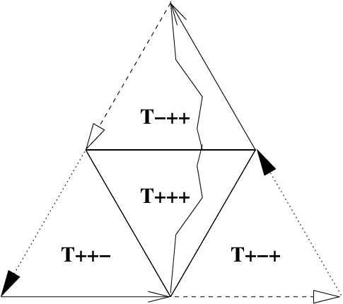
Let . Define to be the set of such that . We will usually abbreviate by and so forth. Note that is what we previously called and . Each is a topological disk and should be visualized as a triangle. Our goal will be to describe the topology of . Pasting together the answer for each , we will find the topology of . The gluing of the T’s is shown in Figure 1.

Fix . Suppose that induces a triangulation of . Label each vertex with either a or a by giving the sign of
We will now describe a collection of polygonal paths in the convex hull of : if is a triangle of such that and have the same sign and has the opposite sign, draw a line segment connecting the midpoints of edges and . If all three vertices have the same sign, do not draw any segments.
Viro’s Patchworking Theorem.
For large enough, there is a homeomorphism between and the convex hull of , taking the corresponding sides of the two triangles to each other and taking the polygonal paths described above to .
Proof.
This is essentially proven in [Viro]. (Viro uses monomials rather than arbitrary members of , but one can check that this is unimportant.) ∎
2.2 Viro’s Theorem for Arbitrary Polyhedral Subdivisions
Now suppose that induces a polyhedral subdivision which is not necessarily a triangulation. Let denote the set of faces of the subdivision; we emphasize that contains the edges and vertices of the subdivision and not only the two dimensional faces. Note that not all the vertices of need be used in .
Let . There is a linear functional such that if and only if . (If is not two dimensional, is not uniquely defined, but this will not be important.)
For , write
where and denotes a member of with . We have if and only if . Set . Intuitively, one should think of as a good approximation to for fixed and large.
We can consider as a function on . (More properly, we should consider as a section of a line bundle on the toric variety corresponding to , but this would introduce concepts we have no need for.) and are clearly both topologically disks of dimension . There is a correct way to choose such homeomorphisms so that the curves paste together to form a closed subspace of .
The following result follows from Viro’s proof:
Theorem 17.
If all of the curves are smooth then, for large enough, there is a homeomorphism from to the convex hull of taking to the subspace of constructed above. Similar comments apply to the other ’s, with appropriate changes of sign in the above construction.
It is clear that Viro’s patchworking theorem is a special case of the above.
The case where the curves are not smooth is still more complicated to describe. In this case, one can not completely describe the topology of in terms of the but one can come close. Namely, one can find a homeomorphism as in the above theorem such that, for large enough, the topology of is a perturbation of the topology of .
We mention this only for the special case where is one dimensional which will be important later.
Lemma 18.
With the notation above, suppose that there is a path through along the edges (one dimensional faces) of such that the sign of changes times along . Then there is a homeomorphism such that, under this isomorphism, meets at most times. Similar results hold for the other ’s.
Proof.
After the preceeding discussion, it is enough to show that, if there are only sign changes in the coefficients of then has at most positive roots. This is Descartes’ rule of signs. ∎
3 Proof of the Main Theorem
The aim of this section is to prove the Main Theorem, which we restate here for the reader’s convenience.
Main Theorem.
Let . Set . If is a strict hive then . If then is a hive.
In both cases, the key to the proofs will be to combine Vinnikov’s Criterion, Viro’s patchworking methods and a little combinatorial reasoning about triangulations.
3.1 If is a Strict Hive then
By Proposition 16, induces the standard subdivision of and by assumption all of the coefficients of are positive. By the Vinnikov Criterion, it is enough to show that has the correct topology for large enough. Thus, we simply must carry out the construction in Viro’s Theorem for the standard triangulation with all of the positive.
The result is shown in Figure 2, where the boundary of the triangle is glued to itself to form as shown in Figure 1 and the bold lines indicate the polygonal paths.

3.2 If then is a Hive
Suppose for the sake of contradiction that is not a hive. By lemma 3 we may perturb each such that is a smooth curve and still in . If we perturb by less than , this will not change the ’s. Thus, without loss of generality, we may assume that is smooth (over or, equivalently, that is smooth for sufficiently large. So Vinnikov’s criterion applies to for sufficiently large.
Let be the polyhedral subdivision induced by . Since is not a coarsening of the standard triangulation, it contains an edge which is not in the standard triangulation. Let this edge run between and . At least one of , and must be greater than . Without loss of generality, suppose that .
Lemma 19.
For some and with , there is a path from to traveling along the edges of and using no more than edges.
Proof.
By starting at and traveling along the edges of in the direction of increasing , we may find a path from to which uses no more than edges of . Similarly, traveling in the direction of decreasing , we may find a path from to which uses no more than edges of . Concatenating these two paths and the edge , we have a path of length no more than . ∎
Let be the path guaranteed by the lemma. Build a model of by gluing together the T’s and identify each T with as in Viro’s Theorem. Then the concatenation of the images of in and form a pseudoline. See Figure 3 for an illustration. The former copy of has at most sign changes, as it has at most edges. The latter copy lies in , where all signs are the same, and thus has no sign changes. So this pseudoline has at most sign changes along it. From Lemma 18, for sufficiently large, there is a pseudoline in , meeting and crossing at most times. This contradicts Vinnikov’s criterion for to lie in .
4 An Explicit Value for
We have seen that the Main Theorem combined with a little logic implies that there exist vectors and such that . In this section, we will find an explicit value for . Our proof will rely on Vinnikov’s criterion but not on patchworking or the Main Theorem, so it may be used to give an alternative proof of the second direction of the Main Theorem.
Specifically, we will prove that:
Proposition 20.
Let . Then
We have the following corollary:
Corollary 21.
In the above notation, one may take
Proof.
Suppose that . We must show that is a hive.
With the above , we have
Thus, the first line of the conclusion of Proposition 20 can be restated as
and similarly for the other lines. Taking s of both sides, we conclude that is indeed a hive. ∎
4.1 Derivatives of Vinnikov Curves
The aim of this section is to prove the following technical lemma:
Lemma 22.
Let . (The subscript means that we are dealing with degree polynomials.) Let , and , . Then
Proof.
Fix . For , set . So traces out the line in joining and . By Vinnikov’s criterion, meets at real points. In other words, the polynomial has distinct real roots. By Rolle’s theorem, has distinct real roots.
But an easy computation shows that
So we have shown that has distinct real zeroes on the line through and .
But was chosen arbitrarily. So we have shown that every line through meets at distinct points. Also, it is clear that has positive coefficients. So, by Vinnikov’s criterion, . ∎
4.2 The Proof
Our proof is by induction on .
Our base case is , so . We may assume without loss of generality that , put and . We are being asked to show that
or, in other words, that
As the diagonal terms of and are positive, this is obvious.
We now continue with the induction. Suppose that . Our proof divides into three cases:
Case 1: .
Case 2: .
This case is precisely analogous to the previous case.
Case 3: .
5 Connection to Honeycombs and Amoebae
5.1 Amoebae
Let be a polynomial. There is a map by . The amoeba of , which we will denote by , is defined to be . If is homogenous, is preserved under translation by and we will abuse notation by using the same sybol to refer to the image of in . We will not aim to discuss the theory of amoebae deeply, see [Mik] for more background.
5.2 NonArchimedean Amoebae
Similarly, let . The tropicalization, also known as the nonarchimedean amoeba, of is . We denote the tropicalization of by .
There is a second description of . Write . Define a piecewise linear functions by . is the nonsmooth locus of this function.
The connection between nonarchimedean amoebae and ordinary amoebae is the following:
Proposition 23.
Let .
where the convergence is in the Hausdorff metric.
5.3 Honeycombs
Now, suppose that is a Vinnikov curve, so that form a hive. Then is what is known as the honeycomb of .
If is a strict hive, its honeycomb will consist of a grid of hexgons, as shown in figure 4. If is a hive which is not strict, some of the edge lengths in the honeycomb will degenerate to ; see [KT] for a precise statemement of the sort of degernerations that can occur. Giving a honeycomb is precisely equivalent to giving a hive modulo .

The boundary of is simply the values of , and on the unbounded rays of . So, the Hive Theorem says that Horn’s additive problem is solvable for , and if and only if there is a honeycomb whose unbounded rays are at positions corresponding to , and .
It is interesting to understand how the hexagonal geometry of the honeycomb relates to the nested curve geometry of the Vinnikov curve. The answer is that the boundary of the amoeba of a Vinnikov curve is made up almost entirely of the real points of the Vinnikov curve except for some segments of length . In the limit as , the limit of the real points of is the same as the limit of the whole amoeba. Thus, is the limit of the image of the real points of under the map. This map folds the jagged arcs of the Vinnikov curve in figure 2 up into a honeycomb, as shown in figure 5. In figure 5, the lines should be precisely superimposed to yield a honeycomb, but have been seperated slightly for clarity.

I am grateful to Mikhalkin for helping me understand the appearance of these amoebae more closely.
6 Behavior in Direct Sums
Let denote the composite map . Let and lie in and respectively. Then we can consider . Then the following is obvious
Proposition 24.
The map constructed in [AMW] preserves direct sums so this also holds for the map .
Let and lie in and respectively. We define the convolution to be the hive defined by
This was proved to be a hive in, for example, [DK] and corresponds to the overlay of honeycombs. It is widely accepted that overlay of honeycombs should correspond to direct sum of matrices.
We now check that the above proposition is consistent with the operator. We state the comparison in terms of power series; there is no difficulty in proving a similar asymptopic result without power series.
Proposition 25.
Let and lie in and . Then
Proof.
Letting , and denote , and respectively, we observed before that . Thus, we have
and
(Here we used that the terms in the sum are all positive.) So
∎
7 Future Directions
7.1 The Ronkin Function
In this section, we will describe a map which has proven to be of use in the theory of amoebas. We will describe reasons to believe that it might be profitable to modify the diagram in section 1.7 by replacing the coordinate-wise by . For more background, see [Mik]. Kenyon and Okounkov (see [KO]) have recently had great success in parameterizing the space of Hanack curves, another type of plane curve with specified topology, by using these methods.
Let (or ). Let . We define
Let , we put
The integral defining always converges, even when the quantity inside the logarithm is sometimes 0. is a convex function. The infimum in the definition of is always finite and attained as long as , and are nonzero.
The following result shows that and have the same asymptotic behavior in the case that interests us.
Proposition 26.
Let with , . Let be the subdivision of induced by . Suppose that is a vertex of a facet of . Then
Proof.
This is an easy consequence of Theorem 2 of [PR]. ∎
Note that the hypothesis of the theorem is satisfied for every when is a strict hive. We now prove two Propositions that suggest may be more important that . We let be the map defined by .
Proposition 27.
If and lie in instead, then, moreover, we have equality for sufficiently large .
Proof.
Let , and and in , and be the polynomials , and . We observed earlier that and it is then clear from the definition that .
Let and let achieve the infimum in the definition of . Consider any and with , and . We have
Taking the maximum over all and , we have the result.
The proof of the last statement is omitted. ∎
Proposition 28.
Let and be the maps deinfed in the first section. Let . Then .
Proof.
By Proposition 3.2 of [FPT], only depends on . Let the roots of , which we know to be negative, be , …, , with .
By Jensen’s theorem,
(The sum is over all such that . Then . The result is now obvious. ∎
7.2 The Existence of Limits
Let denote the composite map by .
We still have not actually constructed a map from or to . By Theorem 13, if is any path in such that exists, this limit is in . The following would be the most elegant way a map could be constructed.
Question 29.
Let be a path in such that exists. Does the limit necessarily exist? Is it dependent only on and not on the choice of path achieving this limit?
I conjecture that the answer to the first question is yes, at least for “nice” paths. On grounds of elegance, the second statement should be true, but I find it hard to imagine how it could occur, as the map depends not only on the asymptopics of the entries in the matrices , and but on those of all their minors. A weaker conjecture is that exists for all . The primary difficulty lies in the map . Because of the analytic nature of its definition, it is difficult to find any data from which to extrapolate.
If such a limiting map does exist then, by Theorem 6, it will be a map from a manifold to a polyhedral cone whose fibers are tori. If are fixed, the fibers will be of the same dimension as the image. This suggests that in some way, we are seeing a degeneration of to a toric variety.
7.3 More Matrices
One can ask to investigate the space , for this is . One can define the map analogously to before. One is now interested in characterizing the space of all polynomials of the form with . We will call a polynomial in a Vinnikov hypersurface. One can also hope to study which we define to be . Write . So .
The first difficulty in this problem is that Theorem 2 is not true for . This is easy to see: giving matrices in involves parameters while giving a polynomial in involves parameters. For and large, .
The if and only if in Vinnikov’s criterion, therefore, can no longer hold, as all of the topological conditions are preserved under perturbing the polynomial . However, one can still derive topological properties of Vinnikov hypersurfaces.
Proposition 30.
Let , …, and set . Then any line meeting meets times. If is smooth, it consists of components that divide into two pieces, with on the contractable portion and possibly one more piece that does not disconnect .
Proof.
This is analogous to the remark after the statement of Vinnikov’s Criterion. ∎
We will say that any hypersurface in with the above topology is a topological Vinnikov hypersurface. It is easy to prove that the derivative of a polynomial cutting out a topological Vinnikov hypersurface itself defines a topological Vinnikov hypersurface, which allows us to prove some easy inequalities by induction as in the proof of theorem 20. I do not know whether the derivative of a Vinnikov hypersurface is a Vinnikov hypersurface.
I have worked out the case of .
Proposition 31.
is defined by the three symmetric permutations of the following inequality:
and the twelve permutations of the following inequality
Note that is a fan, not a cone.
References
- [1]
- [AMW] Alekseev, Meinrenken and Woodward, “Linearization of Poisson Actions and Singular Values of Matrix Products” Ann. Inst. Four. 51 (2001) 1691–1717
- [DK] Danilov and Koshevoy, “Discrete Convexity and Hermitian Matrices”, preprint May 2003.
- [FPT] Forsberg, Passare and Tsikh, “Laurent Determinants and Arrangements of Hyperplane Amoebas”, Advances in Mathematics, 151, 45-70 (2000)
- [Ful] Fulton, “Eigenvalues, Invariant Factors, Highest Weights and Schubert Calculus”, Bull. Amer. Math. Soc. 37 2000
- [GKZ] Gelfand, Kapranov, Zelevinsky, Discriminants, Resultants and Multidimension Discriminants Boston: Birkhäuser 1994
- [HE] Hua and Evens, “Thompson’s conjecture for real semi-simple Lie groups”, preprint, available at http://www.arxiv.org/math.SG/0310098
- [Hor] Horn, “Eigenvalues of Sums of Hermitian Matrices”, Pacific Jour. of Math. 12 (1962), 225-241
- [Jac] Jacobson, Basic Algebra, vol. I and II, New York: W. H. Freeman, 1989
- [Kly] Klyachko, “Random Walks on Symmetric Spaces and Inequalities for Matrix Spectra”, Lin. Alg. App. 319 (2000) 37-59
- [KO] Kenyon and Okounkov, “Planar Dimers and Harnack Curves”, preprint, available at http://www.arxiv.org/math.AG/0311062
- [KT] Knutson and Tao, “The Honeycomb Model of Tensor Products I”, JAMS, 12, no. 4, 1055-1090
- [KTW] Knutson, Tao and Woodward, “The Honeycomb Model of Tensor Products II”, to appear in JAMS, available at http://www.arxiv.org/math.CO/0107011
- [Mik] Mikhalkin, “Amoebas of Algebraic Varieties” Survey for Real Algebraic and Analytic Geometry Conference in Rennes, 2001. Available at www.arxiv.org/math.AG/0108225
- [Pic] Picard, Traité d’Analyse, Vol. II, Paris: Gauthier et Fils, 1893
- [PR] Passare and Rullgard, “Amoebas, Monge-Ampère Measures and Triangulations of the Newton Polytope.” http://www.matematik.su.se/reports/2000/10
- [Vin1] Vinnikov, “Complete Description of Determinantal Representations of Smooth Irreduicible Curves”, Lin. Alg. Appl. 125 103–140 (1989)
- [Vin2] Vinnikov, “Self-Adjoint Determinental Representations of Real Plane Curves”, Math. Ann. 296, 453–479 (1993)
- [Viro] Viro, Patchworking Real Algebraic Varieties, Preprint Uppsala University U.U.D.M. Report 1994:42. Also available at http://www.math.uu.se/ oleg .
- [Wal] Walker, Algebraic Curves New York: Dover, 1950